Higher dimensional Jordan curves

Abstract. We address the question of what is the correct higher dimensional analogue of Jordan curves from the point of view of quantitative rectifiability. More precisely, we show that ‘topologically stable’ sets can be used as covering objects in Analyst’s Travelling Salesman Theorem-type theorems: if $E$ is lower $d$-regular (in a certain suitable sense), then we show that there exists a topologically stable surface $\Gamma$ so that $E\subset\Gamma$ and

$$\operatorname{diam}(E)^{d}+\beta^{d}(E)\approx\mathcal{H}^{d}(\Gamma),$$

where $\beta^{d}$ is a term quantifying the curvature of $E$. A corollary of the main result of this paper and a construction by Hyde [Hyd], is a higher dimensional analogue of Peter Jones TST, valid for any subset of Euclidean space.

1. Introduction

A set $E\subset\mathbb{R}^{n}$ is $d$-rectifiable if it can be covered, up to a set of $\mathcal{H}^{d}$-measure zero, by a countable number of images of $\mathbb{R}^{d}$ under Lipschitz maps $f:\mathbb{R}^{d}\to\mathbb{R}^{n}$. Here $\mathcal{H}^{d}$ denotes the $d$-dimensional Hausdorff measure which can be seen as a surface measure of $E$; recall also that $f:\mathbb{R}^{d}\to\mathbb{R}^{n}$ is $L$-Lipschitz if $|f(x)-f(y)|\leq L|x-y|$ for some $L\geq 1$. Rectifiable sets can be thought of as the measure theoretic analogues of smooth manifolds and they are central in many branches of analysis.

In the past thirty years several theorems appeared which quantify the multiscale behaviour of rectifiable sets. These results were motivated by, and essential to, the solution of long-standing and fundamental questions in analysis, notably the proof of Vitushkin’s conjecture by David [Dav98] or the solution to Painlevé’s problem by Tolsa [Tol03]. This loose family of theorems and techniques came to be known as quantitative rectifiability. The most well-known theorem pertaining to quantitative rectifiability is the so-called Analyst’s Travelling Salesman Theorem (TST), originally proved by Jones in the Inventiones paper [Jon90]: let $E\subset\mathbb{R}^{n}$ be compact. If $A\subset\mathbb{R}^{n}$ ($A$ will be a cube or a ball) and $\operatorname{diam}(A)$ denotes the diameter of $A$, we define $\beta_{E}(A)$ by setting $\beta_{E}(A)\operatorname{diam}(A)$ to be equal to the radius of the smallest cylinder containing $E\cap A$. This is a scale invariant measure of how flat, that is, how close to a line, $E$ is in $A$. Jones’ TST says that $E$ may be covered by a rectifiable curve $\Gamma$ if and only if $\beta(E):=\sum\beta_{E}(3Q)^{2}\ell(Q)<+\infty,$ where the sum is over all dyadic cubes and $\ell(Q)$ is the side length of $Q$. Moreover, if $\Gamma$ is the shortest curve containing $E$, we have

$$\operatorname{diam}(E)+\beta(E)\approx\mathcal{H}^{1}(\Gamma).$$ (1.1)

Jones’ result quantifies in a precise manner how quickly a rectifiable set should become flat as we zoom in through the scales. With time, it found many applications (harmonic measure [BJ94], Kleinian groups [BJ97a], analytic capacity [Tol14], Brownian motion [BJPP97], and graph networks [AS12]).

Jones’ results holds for curves (1-dimensional objects) in space. The extension of quantitative results to $d$-rectifiable sets (with $d>1$) has mostly been developed under the Ahlfors regularity assumption, and with the aim of characterising uniformly rectifiable sets. We give some definitions: a set $E$ is Ahlfors $d$-regular ($d$-AR) if there exists a constant $C$ so that

$$r^{d}/C\leq\mathcal{H}^{d}(E\cap B(x,r))\leq Cr^{d}\quad\mbox{ for }\quad x\in E\quad\mbox{ and }\quad 0<r<\operatorname{diam}(E).$$

(Throughout the article $B(x,r)$ is the open ball centered at $x$ and with radius $r>0$). A set $E$ is called uniformly $d$-rectifiable (or UR) if we can find constants $\theta>0$ and $L\geq 1$ so that for each $x\in E$ and $0<r<\operatorname{diam}(E)$, there exists an $L$-Lipschitz map $f:\mathbb{R}^{d}\to\mathbb{R}^{n}$ so that

$$\mathcal{H}^{d}(E\cap B(x,r)\cap f(B))\geq\theta r^{d},$$

for some ball $B\subset\mathbb{R}^{d}$ also with radius $r$. This is a quantitative notion of rectifiability - it is also stronger: if a set is UR it is also rectifiable. Uniformly rectifiable sets were introduced by David and Semmes in [DS91] and [DS93]. While their motivation was in connection with singular integral operators (SIOs), uniform rectifiability is now an important notion in geometric measure theory and characterising UR sets in terms of their multiscale behaviour has become an active field of research. Many recent important breakthroughs in the theory of singular integrals (for example [NTV14]) and in harmonic measure (see [AHM⁺20]) fundamentally rely on these characterisations.

Currently, there is a move toward results about UR sets beyond the Ahlfors regular setting. Some examples are [DT12], where David and Toro construct Lipschitz parameterisations for Reifenberg flat sets (with holes), or [GST18], which was vital in the solution of Bishop’s Conjecture on harmonic measure [AHM⁺16]. With J. Azzam, we embarked on a program aimed at developing a quantitative theory of rectifiability for lower content $d$-regular sets (or $d$-LCR), building on a previous work by Azzam and Schul [AS18]. A set $E\subset\mathbb{R}^{n}$ is lower content $d$-regular if for each ball $B$ centered on $E$ with radius $r_{B}>0$ we have

$$\mathcal{H}_{\infty}^{d}(E\cap B)\gtrsim r_{B}^{d}.$$

Roughly speaking this means that it cannot concentrate around objects with dimension smaller than $d$. In the joint work with Azzam [AV19] we show that many of the characterisations for UR sets still have a meaning in this more general setting. Some of the results proved here were later used by Azzam ([Azz19]) to give several applications to harmonic measure.

In this paper, building on techniques developed in [AV19], we give a solution to the problem of ‘higher dimensional Jordan curves’, which we presently describe. Jones’ TST has been extended to curves lying in many different spaces (e.g. $\mathbb{R}^{n}$ in [Oki92], Hilbert space in [Sch07], Heisenberg group in [LS16]). However, an Analyst’s TST for higher dimensional objects was not available until recently: Azzam and Schul in [AS18] proved a TST for lower content $d$-regular sets which however looked like

$$\operatorname{diam}(E)^{d}+\beta^{d}(E)\approx\mathcal{H}^{d}(E)+\mathrm{Error}.$$ (1.2)

Here $\beta^{d}(E):=\sum\beta_{E}(3Q)^{2}\ell(Q)^{d}$ and the $\beta$ coefficients are the correct variation of Jones’ original ones (and they measure distance to a $d$-dimensional plane). In contrast to (1.1), observe the appearance of the error term; note also that there is no mention of a covering surface. To prove a TST à la Jones (1.1), one needs to face a fundamental issue: what is a ‘higher dimensional curve’? (Topological balls will not work, for example). Here, we give an answer to this question by considering sets whose $d$-measure is stable under Lipschitz deformations: for each $x$ in the surface $\Sigma$ and each $0<r<\operatorname{diam}(\Sigma)$, we have

$$\mathcal{H}^{d}(B(x,r)\cap\varphi_{t}(\Sigma))\gtrsim r^{d},$$ (1.3)

whenever $\{\varphi_{t}\}_{0\leq t\leq 1}$ is a family of (Lipschitz) deformations homotopic to the identity and so that $\varphi_{t}(y)=y$ if $y\notin B(x,r)$. In English, $\Sigma$ cannot be continuously distorted into a lower dimensional set (just like Jordan curves). Similar topological conditions appeared previously in [DS00] and [Dav04], which also inspired parts of our proof. For this class of sets, which we will call topologically stable $d$-surfaces, we are able to retrieve a TST a lá Jones, (1.1), for lower content regular sets (see Theorems 3.6 and 3.7, Section 3, for precise statements).

Theorem 1.1.

Let $F\subset\mathbb{R}^{n}$ be lower content $d$-regular. There exists a topologically stable $d$-surface such that $F\subset\Sigma$ and

$$\operatorname{diam}(F)^{d}+\beta^{d}(F)\approx\mathcal{H}^{d}(\Sigma).$$

If $\beta^{d}(F)<+\infty$ then $F$ and $\Sigma$ are $d$-rectifiable.

Recently Hyde ([Hyd]) proved that for any set $E\subset\mathbb{R}^{n}$, if there is a $d$ so that $\beta^{d}(E)<+\infty$ (here, again, the coefficients are the appropriate variant for the problem), then one can construct a lower content $d$-regular set $F$ so that $E\subset F$. Moreover it holds that $\beta(E)\approx\beta(F)$. Hence, a corollary of Theorem 1.1 together with Hyde’s construction is a full higher dimensional Travelling Salesman Theorem for general sets.

Corollary 1.2.

Let $E\subset\mathbb{R}^{n}$. Then if there exists a $d$ so that $\beta^{d}(E)<\infty$, there exists $d$-LCR set $F$ and a (rectifiable) topologically stable $d$-surface $\Sigma$ so that $E\subset F\subset\Sigma$ and

$$\operatorname{diam}(E)^{d}+\beta^{d}(E)\approx\mathcal{H}^{d}(\Sigma).$$

We conclude that topologically stable surfaces can be conceived as higher dimensional analogues to ‘Jordan curves’ (from a TST perspective).

1.1. Relevance and more applications

The reader may understandably wonder whether Theorem 1.1 is at all interesting or useful. The author thinks it is interesting in the sense that, behind it, there is a natural question: what should a ‘higher dimensional curve’ be? Although as stated such a question is imprecise and open to very many answer, if we add ‘from the point of view of the Analyst’s TST’, it takes a decidedly more precise meaning. As for the usefulness of the result, we provide a few more applications (with the hope that more will come). We state the results rather imprecisely, to convey some ideas. We postpone details to Section 4.

• We call a set uniformly non $d$-flat if the $d$-dimensional $\beta$-coefficients (as defined in (3.3)) are large at all scales. As first application of our main result, we show that if $E$ is $d$-stable and uniformly non $d$-flat, then it must have Hausdorff dimension larger than $d$. This result was proven by David in [Dav04] under stronger topological assumptions. We provide a quantitative strengthening of David’s result (under a weaker topological condition) which gives a precise dependence between $\beta$-coefficients and dimension. See Theorem 4.2, Section 3.

• In [Sem95], Semmes stated the following guiding principle to understand the relation between the topology of some set, and its ‘mass’ distribution: ‘Suitable topological conditions on a space in combination with upper bounds on the mass often implies serious restrictions on the geometric complexity of the space.’ As a second application, we give a result that makes this principle precise: a topologically stable $d$-surface which is also upper regular is uniformly rectifiable. This result is similar to the main result in [DS00]. See Corollary 4.5, Section 3.

1.2. Sketch of the proof

We give a brief idea of the proof. As a first step, we apply a construction from [AV19] which gives a coronisation of a $d$-stable surface $E$ by Ahlfors $d$-regular sets. One should imagine such a construction as a dyadic approximation of $E$ at certain scales. Next, following ideas coming from the proofs in [Dav04], we show that, first, the topological condition transfers from $E$ to the approximating sets. The fundamental observation is this: because the approximating sets are Ahlforse regular and satisfy the topological condition, they turn out to have large intersection with quasiminimal sets. By the main result in [DS00], sets of this type are (locally) uniformly rectifiable. This will give certain estimates on the $\beta$-coefficients, which will then be transferred back to $E$, to obtain one direction of Theorem 1.1. The other direction follows from the main result in [AS18].

1.3. Structure of the paper

In Section 2 we gather some notation which will be used throughout the paper. In Section 3 we state precisely the main result (Theorem 3.6) and the definition of the topological condition (Definition 3.5). We give the precise statements of the two applications mentioned above (Theorem 4.2 and Corollary 4.5) together with the relevant definitions in Section 4. In Section 5 we give some remarks on the choice of the topological condition and show that some perhaps better known types of surfaces falls withing this category. In Section 7 we start the proof in earnest with some preliminary reductions and by applying the corona construction of [AV19]. In Section 8 we define a variant of the topological condition and show that it is ‘inherited’ from $E$ by the approximating sets coming from [AV19]. Section 9 introduces a fundamental tool, Federer-Fleming projections. In Section 10 we show that the above mentioned ‘inheritance’ effectively happens. Section 11 presents a further family of approximating sets. In Sections 12 and 13 we show that the approximating sets lie close to a uniformly rectifiable set. Sections 15 and 16 concludes the proof via some $\beta$-coefficients estimates. In Section 17 we construct a stable surface, given any lower content regular set. In Section 18 we give a proof of the application to uniformly non-flat sets mentioned above.

1.4. Acknowledgements

The bulk of this work was done while I was a PhD student at Edinburgh under Jonas Azzam. I thank him for suggesting the problem, for his help, support and patience. I would also like to thank PCMI/IAS and the organisers of the graduate school of 2018 on Harmonic Analysis: it was here that I learnt many tools used in this paper, as explained by Guy David (whom I also thank for the clear explanations). Some revision was done while a postdoc under Tuomas Orponen, whom I thank for his support. I finally thank Matt Hyde for explaining to me his results.

2. Preliminaries

We gather here some notation and some results which will be used later on. We write $a\lesssim b$ if there exists a constant $C$ such that $a\leq Cb$. By $a\approx b$ we mean that there exists a constant $C>0$ so that $a\lesssim_{C}b\lesssim_{C}a$. If the constant $C$ depends on some parameter, say $\epsilon$, than we will write $a\lesssim_{\epsilon}b$ or $a\approx_{\epsilon}b$. If we have no interest in keeping track of parameter and or constant, we will simply write $a\lesssim b$ or $a\approx b$. If $A$ is a subset of some set $B$, then $A^{c}=B\setminus A$. For sets $A,B\subset\mathbb{R}^{n}$, we let

$$\mathop{\mathrm{missing}}{dist}(A,B):=\inf_{a\in A,b\in B}|a-b|.$$

The diameter of a set $A$ is defined as $\operatorname{diam}(A):=\sup_{x,y\in A}|x-y|$. For a point $x\in\mathbb{R}^{n}$ and a subset $A\subset\mathbb{R}^{n}$, $\mathop{\mathrm{missing}}{dist}(x,A):=\mathop{\mathrm{missing}}{dist}(\{x\},A)=\inf_{a\in A}|x-a|.$ We write $B(x,r):=\{y\in\mathbb{R}^{n}\,|\,|x-y|<r\}.$ Sometimes we will denote a ball simply by $B$; in this case its radius will be $r(B)$ or $r_{B}$ and its center $x_{B}$ or $z_{B}$.

2.1. Measure, content, Choquet integrals

For a set $A\subset\mathbb{R}^{n}$, $d\geq 0$ and $\delta>0$, write

$$\mathcal{H}_{\delta}^{d}(A)=\inf\left\{\sum_{i}\operatorname{diam}(A_{i})^{d}\quad|\quad A\subset\bigcup_{i}A_{i}\quad{\rm and}\quad\operatorname{diam}(A_{i})<\delta\right\}.$$

The the $d$-dimensional Hausdorff measure of $A$ is given by $\mathcal{H}^{d}(A)=\lim_{\delta\to 0}\mathcal{H}^{d}_{\delta}(A)$. The $d$-dimensional Hausdorff content, on the other hand, is given by

$$\mathcal{H}^{d}_{\infty}(A)=\inf\left\{\sum_{i}\operatorname{diam}(A_{i})^{d}\quad|\quad A\subset\bigcup_{i}A_{i}\right\}.$$ (2.1)

For a function $f:\mathbb{R}^{n}\to[0,\infty)$, a set $A\subset\mathbb{R}^{n}$ and $0<p<\infty$, the $p$-Choquet integral with respect to Hausdorff content $\mathcal{H}^{d}_{\infty}$ is defined as

$$\int_{A}f(x)^{p}\,d\mathcal{H}^{d}_{\infty}(x):=\int_{0}^{\infty}\mathcal{H}^{d}_{\infty}\left(\left\{x\in A\,|\,f(x)>t\right\}\right)\,t^{p-1}\,dt.$$ (2.2)

Choquet integrals satisfy all the standard linearity properties of integral with respect to measures. We will highlight throughout the proofs when certain properties of Choquet integrals are needed. We (will) refer the reader to Section 2.1 of [AS18] (‘Hausdorff measure and content’) for the relevant lemmas. Following (2.2), we will write

$$\beta_{E}^{d,p}(B)=\inf_{L}\left(\int_{B}\left(\frac{\mathop{\mathrm{missing}}{dist}(y,L)}{r(B)}\right)^{p}\,d\mathcal{H}^{d}_{\infty}(y)\right)^{\frac{1}{p}},$$

where $B$ is a ball. We will often write

$$\beta_{E}^{d,p}(x,r):=\beta_{E}^{d,p}(B(x,r)).$$ (2.3)

2.2. Cubes, stopping times

2.2.1. Dyadic cubes and skeleta

For $j\in\mathbb{Z}$, we will denote by $\Delta_{j}$ the family of dyadic cubes with side length $2^{-j}$. We also set

$$\Delta:=\bigcup_{j\in\mathbb{Z}}\Delta_{j}.$$

For a set $A\subset\mathbb{R}^{n}$, we put $\Delta(A):=\left\{I\in\Delta\,|\,I\cap A\neq\varnothing\right\}.$ For a cube $I\in\Delta$ and an integer $1\leq k<d$, we write

$$\partial_{k}I$$ (2.4)

to denote the $k$-dimensional skeleton of $I$. We also set

$${\mathcal{S}}_{j,k}:=\bigcup_{I\in\Delta_{j}}\partial_{k}I.$$ (2.5)

Let us remark that for a set $V$, we write $\partial I$ to mean the standard boundary of $V$; so in particular $\partial I=\partial_{n-1}I$.

2.2.2. Christ-David cubes

In the (sloppy) statement of Theorem 1.1, the summation was over a family of cubes $\mathcal{D}$. These are not the standard dyadic cubes; however the reader may think of them as dyadic ‘intrinsic’ dyadic cubes of a set $E$. We may refer to these cubes as Christ-David cubes, to distinguish them from the dyadic cubes. As it would be cumbersome to use write each time ‘Christ-David cube’, in some sections we will simply call them cubes. However, there will always be a notational difference:

• Dyadic cubes will always be denoted by $I,J$.

• On the other hand, we will denote Christ-David cubes with $Q,P,R$.

The following theorem gives the existence Christ-David cubes. A first version of the theorem is by David in [Dav88]; subsequent versions appeared in [Chr90] and [HM12]. Before stating the theorem, recall that a metric space is doubling if there exists a number $N$ so that any ball can be covered by $N$ balls of half the radius. We will apply Theorem 2.1 below with $X=E$, where $E$ is a subset lying in the Euclidean space $\mathbb{R}^{n}$; in particular $E$ (as metric space) will always be doubling.

Theorem 2.1.

Let $X$ be a doubling metric space. Let $X_{k}$ be a nested sequence of maximal $\lambda^{k}$-nets for $X$ where $\lambda<1/1000$ and let $c_{5}=1/500$. For each $n\in{\mathbb{Z}}$ there is a collection $\mathcal{D}_{k}$ of ‘cubes’, which are Borel subsets of $X$ such that the following hold.

1. For every integer $k$, $X=\bigcup_{Q\in\mathcal{D}_{k}}Q$.

2. If $Q,Q^{\prime}\in\mathcal{D}=\bigcup\mathcal{D}_{k}$ and $Q\cap Q^{\prime}\neq\emptyset$, then $Q\subseteq Q^{\prime}$ or $Q^{\prime}\subseteq Q$.

3. For $Q\in\mathcal{D}$, let $k(Q)$ be the unique integer so that $Q\in\mathcal{D}_{k}$ and set $\ell(Q)=5\lambda^{k(Q)}$. Then there is $z_{Q}\in X_{k}$ so that

   $$B(z_{Q},c_{5}\ell(Q))\subseteq Q\subseteq B(z_{Q},\ell(Q))$$ (2.6)

   and $X_{k}=\{z_{Q}\;|\;Q\in\mathcal{D}_{k}\}$.

We now set some notation. For $Q\in\mathcal{D}$, we denote by $B_{Q}$ the ball $B(z_{Q},\ell(Q))$. Also, some jargon: for a cube $Q\in\mathcal{D}$, we denote $\mathcal{D}(Q)$ the family of cubes in $\mathcal{D}$ which are also subsets of $Q$. If $Q\in\mathcal{D}_{k}$, then the cubes $Q^{\prime}\in\mathcal{D}_{k+1}(Q)$ are called the children of $Q$, while $Q$ is the (unique) parent cube of any $Q^{\prime}\in\mathcal{D}_{k+1}(Q)$, or the ancestor of any $Q^{\prime}\in\mathcal{D}(Q)$. For a Christ-David cube $Q$, the collection of its children is denoted by $\mathrm{Child}(Q)$. Two cubes having the same parent are surprisingly called siblings.

2.2.3. Stopping times

Later on we will need to partition $\mathcal{D}$ into subfamilies of cubes. These subfamilies will be often called stopping-time regions and are defined as follows.

Definition 2.2.

A collection of Christ-David cubes $\mathsf{S}\subseteq\mathcal{D}$ is a stopping-time region or tree if the following hold:

1. There is a cube $Q(\mathsf{S})\in\mathsf{S}$ that contains every cube in $\mathsf{S}$.

2. If $Q\in\mathsf{S}$, $R\in\mathsf{S}$, and $Q\subseteq R\subseteq Q(\mathsf{S})$, then $R\in\mathsf{S}$.

3. If $Q\in\mathsf{S}$ and there is $Q^{\prime}\in\mathrm{Child}(Q)\backslash\mathsf{S}$, then $\mathrm{Child}(Q)\subset\mathsf{S}^{c}$.

Definition 2.3.

Given a family ${\mathscr{F}}$ of cubes (either dyadic or Christ-David), the subcollection of maximal cubes from ${\mathscr{F}}$ is the subset of ${\mathscr{F}}$ composed of cubes which have the largest sidelength and such that any other cube in ${\mathscr{F}}$ is contained in one of the cubes in this subcollection.

2.3. Constants

We collect here all the various different constants that will be used throghout the paper.

1. $n,d$: the dimension of the ambient space and of the set under consideration, respectively.

2. $\mathsf{c}_{1}$: the lower content regularity constant. It first appears in 3.1.

3. $\mathsf{A}$: it determines how much we are inflating the ball where we are measuring the $\beta$ number. It first appears in Theorem 3.2.

4. $\mathsf{C}_{0}$: it determines the expansion of the ball where we are measuring the BWGL. It first appears in Theorem 3.2.

5. $\epsilon$: tolerance parameter in BWGL (see (3.5)), and in the definition of Reifenberg-flatness.

6. $\mathsf{c}_{2}$ and $\mathsf{c}_{3}$: constants in the definition of the modified content, first appearing in (3.25).

7. $c_{1}$: constant appearing in the definition of Semmes surfaces, see Definition 5.1.

8. $C_{1}$: expansion factor of top cubes in Lemma 7.7.

9. $\tau$: smoothing parameter in Lemma 7.7.

10. $k_{0}$: generation parameter in Lemma 7.7.

11. $M$: constant for the stopping time in the construction of Lemma 7.7.

12. $\lambda$: nets parameter in Theorem 2.1.

13. $c_{5}$: containment parameter in Theorem 2.1.

14. $r_{0},\alpha_{0},\eta_{0},\delta_{0},\gamma_{0}$: parameters of the topological condition (TC).

15. $r_{1},\alpha_{1},\eta_{1},\delta_{1}$: parameters for the skeletal topological condition (see (8.1)).

16. $C_{2}$: constant of the skeletal topological condition. See Definition 8.1.

17. $\mathsf{C}_{3}$: Ahlfors regularity constant of the approximating set $E_{R}$ (and of $E_{\rho})$. See the paragraph above Lemma 11.3.

18. $\rho$: scale parameter of the approximating set $E_{\rho}$. See (11.3).

19. $\sigma$: scale parameter for the construction of the domain of the fucntional $J$. See (12.4).

20. $M$: large constant in the functional $J$ (not the same $M$ as above!). See 12.22.

21. $c_{2}$: small constant in the definition of $M$ (see (12.22)).

22. $k$: quasiminimality: Hausdorff measure constant. See (13.1) and (13.8).

23. $\delta$: quasiminimality: locality constant. See (13.1) and the properties of the Lipschitz deformation $\phi$ (13.5)-(13.7).

24. $c_{3}$: small constant in the choice of $\delta$. See (13.16).

25. $C_{4}$: inflation constant for the $\beta$ numbers on $Z_{Q}$.

3. Actual theorems

In this section we state our main results and those of Azzam and Schul and of Hyde in a precise manner. Note that all the statements below are local, that is, they concern an arbitrary Christ-David cube of the relevant set.

3.1. Azzam and Schul’s TST

3.1.1. Issues in higher dimensions

It has been mentioned in the introduction that it took quite a while to arrive at a higher dimensional version of the TST. There are two reasons for this.

1. The first is that which motivates the current paper: what to use as a covering surface in higher dimensions? One could legitimately think about, for example, topological spheres; see Figure 1 for why this would not be a good candidate.

2. The second issue is technical in nature: in any situation where one is dealing with sets of dimension larger than one, Jones’ $\beta_{E,\infty}$ coefficients (as defined in the Introduction) become rather useless: in his PhD thesis, X. Fang constructed a codimension one Lipschitz graph $G$ in $\mathbb{R}^{3}$ with $\beta_{\infty}^{2}(G)=\infty$, see [Fan90] or Example 1.16 in [AS18]. A further version of Jones’ coefficients was introduced by David and Semmes in [DS91]. We will define them later on; for the moment it will suffice to say this: David and Semmes’ coefficients make sense for ‘higher dimensional’ sets, as long as such sets are a priori Ahlfors regular. Ahlfors regularity is a size condition which impose a certain relationship between the diameter of a portion of the set and its mass. However, Jones’s theorem does not assume this; indeed, $E$ need not to have a priori finite $d$-dimensional measure, let alone be Ahlfors regular. Thus, a new type of coefficient measuring flatness is needed.

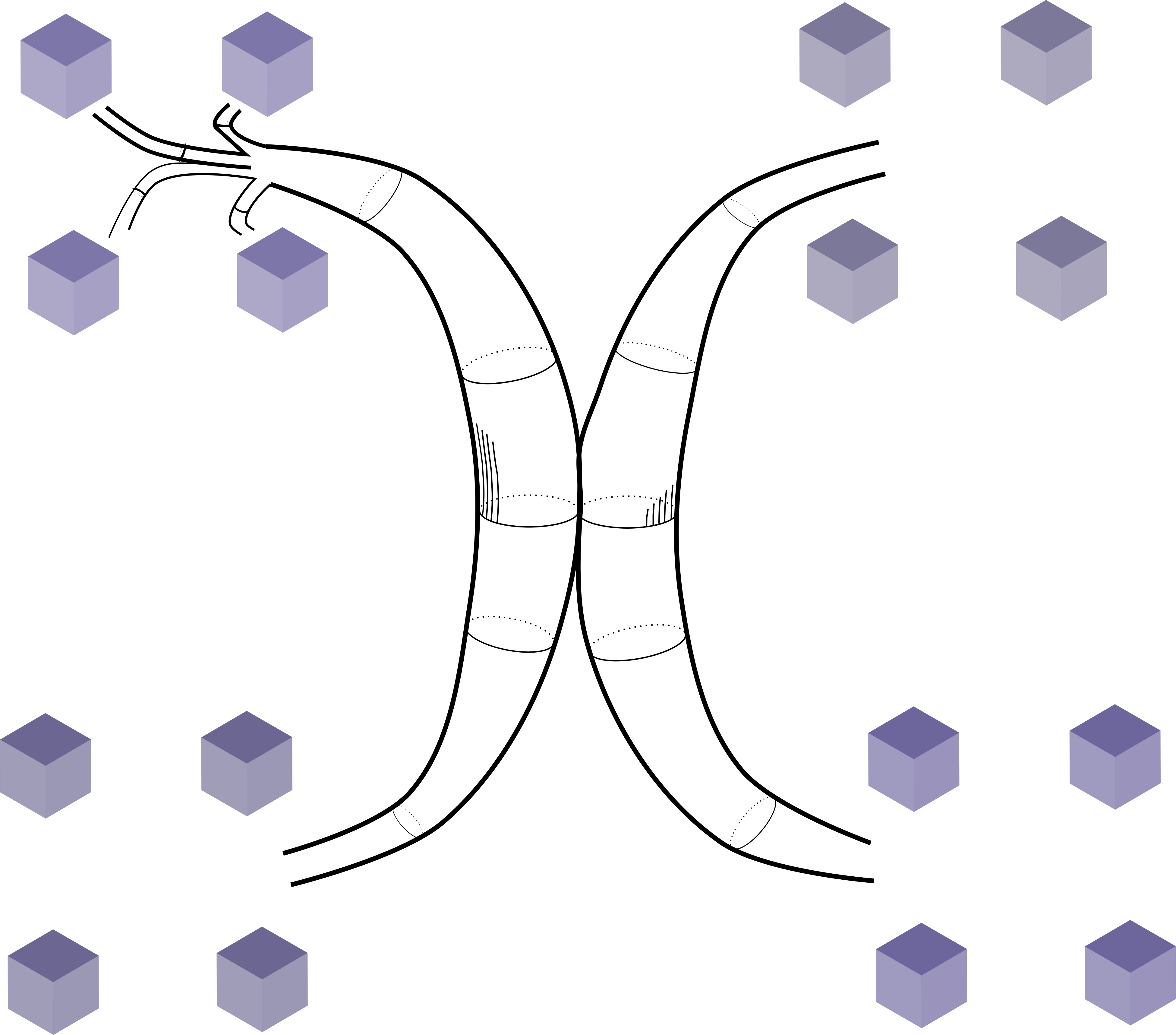
Figure 1. Given the $2$-dimensional 8-corner Cantor set in $\mathbb{R}^{3}$, one can construct a $2$-dimensional surface with finite measure, so that the closure of this surface will contain the Cantor set and will be homeomorphic to the $2$-sphere.

Notwithstanding these difficulties Azzam and Schul proved in [AS18] a version of Jones’ theorem for sets of dimension larger than one in Euclidean space.

1. To deal with the first difficulty, Azzam and Schul decided to focus on obtaining a quantitative result of type (1.1) directly for a set $E$ lying in $\mathbb{R}^{n}$, without trying to find a ‘covering object’. To be able to make some progress, they imposed on $E$ a size condition called lower content regularity.

   Definition 3.1.

   We say that a set $E\subset\mathbb{R}^{n}$ is lower content $d$-regular with constant $\mathsf{c}_{1}\leq 1$, or lower content $(d,\mathsf{c}_{1})$-regular, if

   $$\mathcal{H}^{d}_{\infty}(B(x,r)\cap E)\geq\mathsf{c}_{1}r^{d}$$ (3.1)

   for all $(x,r)\in E\times(0,\operatorname{diam}(E))$.

   The symbol $\mathcal{H}^{d}_{\infty}$ represents Hausdorff content, which has been defined in (2.1). Roughly speaking, lower content regularity prevents a set $E$ to concentrate around objects of dimension smaller than $d$. It is a natural assumption to impose on $E$, and it appears, in a form or another, in works on harmonic measure for example (see [AAM19], [ABH⁺19], [Azz19]).

2. To deal with the second difficulty, Azzam and Schul introduced the following variant of the $L^{p}$-type $\beta$ coefficients. For a set $B\subset\mathbb{R}^{n}$

   $$\beta_{E}^{d,p}(B)=\inf_{L}\left(\int_{B}\left(\frac{\mathop{\mathrm{missing}}{dist}(y,L)}{r(B)}\right)^{p}\,d\mathcal{H}^{d}_{\infty}(y)\right)^{\frac{1}{p}},$$ (3.2)

   $$\beta_{E}^{d,p}(B):=\inf_{L}\left(\frac{1}{r^{d}}\int_{0}^{1}\mathcal{H}^{d}_{\infty}(\{y\in B\cap E\,|\,\mathop{\mathrm{missing}}{dist}(y,L)>t\,\operatorname{diam}(B)\})t^{p-1}\,dt\right)^{\frac{1}{p}},$$ (3.3)

   where the infimum is taken over all affine $d$-planes $L$ in $\mathbb{R}^{n}$. The integral on the right hand side of (3.3) is a Choquet integral. Azzam and Schul chose $\mathcal{H}^{d}_{\infty}$ to define their $\beta$ coefficients because $\mathcal{H}^{d}_{\infty}$ does not blowup. Indeed, for any set $E$, we always have that $\mathcal{H}^{d}_{\infty}(E)\lesssim\operatorname{diam}(E)^{d}$, even when the Hausdorff dimension of $E$ is larger than $d$. We refer the reader to Examples 1.14, 1.15 and 1.16 in [AS18] for some examples which motivate their choice of $\beta$-coefficients.

3.1.2. What Azzam and Schul proved

We need to introduce a little more notation. Given two closed sets $E$ and $F$, and $B$ a set we denote

$$d_{B}(E,F)=\frac{2}{\operatorname{diam}B}\max\left\{\sup_{y\in E\cap B}\mathop{\mathrm{missing}}{dist}(y,F),\sup_{y\in F\cap B}\mathop{\mathrm{missing}}{dist}(y,E)\right\}$$ (3.4)

Recall that, by Theorem 2.1, for each Christ-David cube $Q\in\mathcal{D}$, there is a ball $B_{Q}$ centered on, containing, and of comparable size to, $Q$. For $\mathsf{C}_{0}>0$, and $\epsilon>0$, let

$${\mathsf{BWGL}}(\mathsf{C}_{0},\epsilon)=\{Q\in\mathcal{D}|\;\;d_{\mathsf{C}_{0}\,B_{Q}}(E,P)\geq\epsilon\;\;\mbox{ for all $d$-planes }P\}.$$ (3.5)

We can now state the result from [AS18] (Theorems I and II there). This is the estimate which appeared in the Introduction as (1.2). To be sure, our phrasing is slightly different to the original one, but the interested reader can find a justification of this reformulation in the Appendix of [AV19].

Theorem 3.2 ([AS18], Theorems I and II).

Let $1\leq d<n$ and $E\subseteq{\mathbb{R}}^{n}$ be a closed set. Suppose that $E$ is lower content $d$-regular with constant $\mathsf{c}_{1}$ and let $\mathcal{D}$ denote the Christ-David cubes for $E$. Let $\mathsf{C}_{0}>1$. Then there is $\epsilon>0$ small enough so that the following holds. Let $1\leq p<p(d)$ where

$$p(d):=\left\{\begin{array}[]{cl}\frac{2d}{d-2}&\mbox{if }d>2\\ \infty&\mbox{if }d\leq 2\end{array}\right..$$ (3.6)

For $R\in\mathcal{D}$, let

$${\rm BWGL}(R):={\rm BWGL}(R,\epsilon,\mathsf{C}_{0})=\sum_{Q\in{\mathsf{BWGL}}(\epsilon,\mathsf{C}_{0})\atop Q\subseteq R}\ell(Q)^{d},$$ (3.7)

and

$$\textup{{BETA}}_{E,d,p,\mathsf{A}}(R):=\sum_{Q\in\mathcal{D}(R)}\beta_{E}^{d,p}(\mathsf{A}\,B_{Q})^{2}\ell(Q)^{d}.$$ (3.8)

Then for $R\in\mathcal{D}$,

$$\mathcal{H}^{d}(R)+{\rm BWGL}(R,\epsilon,\mathsf{C}_{0})\approx_{\mathsf{A},n,\mathsf{c}_{1},p,\mathsf{C}_{0},\epsilon}\textup{{BETA}}_{E,\mathsf{A},p}(R)+\ell(R)^{d}.$$ (3.9)

Let us recall that the coefficients $\beta_{E}^{p,d}$ are those defined in (3.3). These coefficients enjoy some standard properties such as a sort of monotonicity with respect to balls’ radii and an ‘ability’ to jump between two close-by sets without changing their value too dramatically. We will highlight when we use these properties and cite the relevant lemmas from [AS18].

Remark 3.3.

The presence of $\rm BWGL(E)$ in (3.9) is natural: in Jones’s theorem the right-hand-side only contains the length of the covering curve; now, a curve has no holes. However, $E$ may very well be quite broken (even while being lower content regular). Thus, if we imagine our set $E$ being covered by ‘a higher dimensional curve’ $\Gamma$, we would have $\mathcal{H}^{d}(\Gamma)\approx\mathcal{H}^{d}(E)+\text{BWGL}(E)$, where $\text{BWGL}(E)\approx\mathcal{H}^{d}(\Gamma\setminus E)$ (see Figure 2).

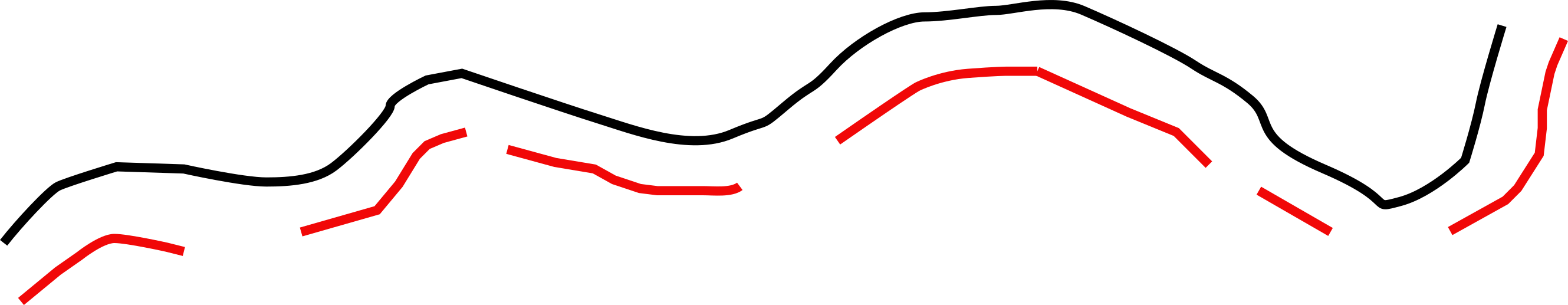
Figure 2. A covering curve picks up the holes in the set (left). In the absence of a ‘higher dimensional curve’, the term BWGL accounts for the holes (right).

3.2. Stable $d$-surfaces

We now define precisely the topological condition mentioned in (1.3). Our definition is a weaker version of that of David in [Dav04]. Let $E$ be a closed subset of $\mathbb{R}^{n}$.

Definition 3.4 (Allowed Lipschitz deformations with parameter $\alpha_{0}$).

Fix a constant $0<\alpha_{0}<1$. Consider a one parameter family of Lipschitz maps $\{\varphi_{t}\}$, $0\leq t\leq 1$, defined on $\mathbb{R}^{n}$. For $x\in E$ and $r>0$, we say that $\{\varphi_{t}\}_{0\leq t\leq 1}$ is an allowed Lipschitz deformation with parameter $\alpha_{0}$, or an $\alpha_{0}$-ALD, if it satisfies the following four conditions:

$$\varphi_{t}(\overline{B}(x,r))\subset\overline{B}(x,r)\mbox{ for each }t\in[0,1];$$ (3.10)

$$\mbox{ for each }y\in\mathbb{R}^{n},\,t\mapsto\varphi_{t}(y)\mbox{ is a continuous function on }[0,1];$$ (3.11)

$$\varphi_{0}(y)=y\mbox{ for all }y\in\mathbb{R}^{n}\mbox{ and }\varphi_{t}(y)=y\mbox{ for }t\in[0,1]\mbox{ whenever }y\in\mathbb{R}^{n}\setminus B(x,r);$$ (3.12)

$$\mathop{\mathrm{missing}}{dist}(\varphi_{t}(y),E)\leq\alpha_{0}r\mbox{ for }t\in[0,1]\mbox{ and }y\in E\cap B(x,r).$$ (3.13)

Thus if we perturb a set $E$ in a ball $B(x,r)$ with an $\alpha_{0}$-ALD, what we do is effectively to move in a thin tube around $E\cap B(x,r)$. The topological condition that we impose on $E$ is the following.

Definition 3.5 (Stable $d$-surface).

Fix five parameters:

$$r_{0},\mbox{ the scale parameter;}$$ (3.14)

$$\alpha_{0},\mbox{ the distance parameter;}$$ (3.15)

$$\delta_{0},\mbox{ the lower regularity parameter; }$$ (3.16)

$$\eta_{0},\mbox{ the boundary parameter;}$$ (3.17)

$$\gamma_{0},\mbox{ the `other ball' parameter.}$$ (3.18)

We say that a closed set $E$ is a (topologically) stable $d$-surface with parameters $r_{0},\alpha_{0},\delta_{0}$, $\eta_{0}$ and $\gamma_{0}$, if for each $x_{0}\in E$ and $0<r<r_{0}$ we can find a ball $B$ such that

$$B\mbox{ is centered on }E;$$ (3.19)

$$B\subset B(x_{0},r);$$ (3.20)

$$\gamma_{0}r\leq r(B)\leq r;$$ (3.21)

$$\mathcal{H}^{d}\left(B(x_{B},(1-\eta_{0})r(B))\cap\varphi_{1}(E)\right)\geq\delta_{0}r^{d},$$ (TC)

whenever $\varphi_{t}$ is an $\alpha_{0}$-ALD relative to $(x_{B},r(B))$. We will refer to the above condition on $E$ as the ‘topological condition’, or TC for short.

This definition looks rather technical. However there are plenty of stable surface. An obvious example is that of a curve. Also a square in the plane is a stable $1$-surface, simply because the left hand side of (TC) is always infinite. We will present more interesting examples in Section 5, namely sets satisfying the so called Condition B and Reifenberg flat sets. On the other hand, the surface depicted in Figure 1 (the many-tentacled octopus) is not a stable $2$-surface: at any scale one can shrink the diameter of the tubes as much as one wants (note that there is no uniform bound on the Lipschitz constant of an ALD). By doing so, one can make the Hausdorff $2$-measure of the surface of the tubes arbitrarily small, hence breaking (TC)

3.3. Statement of the main result

We now state Theorem 1.1 as the following (more precise) statement.

Theorem 3.6.

Assume that $1\leq d<n$. Let $E\subset\mathbb{R}^{n}$ be a stable $d$-surface with parameters $r_{0},\alpha_{0},\delta_{0}$ and $\eta_{0}$ and let $\mathcal{D}$ be its Christ-David cubes. Let $Q_{0}\in\mathcal{D}$ be an arbitrary cube satisfying $\ell(Q_{0})\leq r_{0}$ and let $\mathsf{A}$ be a sufficiently large positive constant. Take $1\leq p<p(d)$ with

$$p(d):=\left\{\begin{array}[]{cl}\frac{2d}{d-2}&\mbox{if }d>2\\ \infty&\mbox{if }d\leq 2\end{array}\right.$$

Then it holds that

$${\rm diameter}(Q_{0})^{d}+{\rm BETA}(Q_{0})\approx\mathcal{H}^{d}(Q_{0}),$$ (3.22)

where

$${\rm BETA}(Q_{0})={\rm BETA}_{E,\mathsf{A},p,d}(Q_{0}):=\sum_{Q\in\mathcal{D}(Q_{0})}\beta_{E}^{d,p}(\mathsf{A}B_{Q})^{2}\ell(Q)^{d},$$ (3.23)

and where the constant behind the symbol $\approx$ depends on the parameters of $\eqref{e:TC}$ ($\alpha_{0},\delta_{0},r_{0},\eta_{0}$, $\gamma_{0}$), on $\mathsf{A}$, on $p$, and on the dimensional parameters ($d$, $n$).

The assumption that $\ell(Q_{0})\leq r_{0}$ is a natural one and cannot be avoided. Assuming the topological condition from a certain scale, i.e. from $r_{0}$, means that at larger scale there could be holes. This would make the term $\text{BWGL}(Q_{0})$ come back. The assumption that $E$ is closed is relevant, but not restrictive; in fact we have that $\mathcal{H}^{d}(E)=\mathcal{H}^{d}(\overline{E})$. A corollary of Theorem 3.6 is the following.

Corollary 3.7.

Fix $\epsilon>0$ sufficienlty small and $\mathsf{C}_{0}>1$. Let $E\subset\mathbb{R}^{n}$ be a lower content $(d,\mathsf{c}_{1})$-regular set (see (3.1)). Let $Q_{0}\in\mathcal{D}$. There exists a set $\Sigma=\Sigma(Q_{0},\epsilon,\mathsf{C}_{0})$ such that

1. $Q_{0}\subset\Sigma$.

2. $\Sigma$ is a stable $d$-surface with parameters $r_{0}=\ell(Q_{0})$, $\eta_{0},\gamma_{0},\alpha_{0}$ sufficiently small with respect to $\epsilon>0$ and $\delta_{0}$ sufficiently small depending on $\eta_{0},\alpha_{0},\gamma_{0}$ and $d$.

3. We have the estimate

   $${\rm diameter}(Q_{0})^{d}+{\rm BETA}_{E,d,p,\mathsf{A}}(Q_{0})\approx\mathcal{H}^{d}(\Sigma),$$ (3.24)

   where ${\rm BETA}_{E,d,p,\mathsf{A}}(Q_{0})$ is as in (3.23) and the constant behind the symbol $\approx$ depend on $n,d,\mathsf{c}_{1},\epsilon,\mathsf{C}_{0},\mathsf{A}$ and $(\alpha_{0},\eta_{0},\gamma_{0},\delta_{0},\gamma_{0})$.

The corollary above gives a TST for lower content regular sets, and uses as ‘curves’ stable $d$-surfaces. Glaringly, one would like to drop the lower content regularity assumption. The following construction, due to Hyde, does precisely this.

3.4. Hyde’s construction

In the recent paper [Hyd], Hyde shows that for any set $F\subset\mathbb{R}^{n}$, one can construct a lower content $d$-regular set $E$ with some parameter $\mathsf{c}_{1}$ such that $F\subset E$ and, importantly, one has comparability between the ${\rm BETA}$ term of $F$ and that $E$ (as was mentioned in the introduction). The removal of the lower content regularity assumption presents an important issue here - we spell it out for clarity: how to pick up the geometry of a set which has potentially very little mass? The ($d$-dimensional) $\beta$ coefficients of Azzam and Schul (see (3.3)) will always return a small number if computed on a set with small $d$-dimensional content, even if the set is extremely non-flat. It is clear then that one needs to devise a different ‘geometry detector’ to say something useful about sets which have no lower bounds on their mass. Hyde’s idea is simple yet ingenious: he defines a different content, denoted by ${\widetilde{\mathcal{H}}^{d}_{\infty}}$, with respect to which any set $E$ becomes lower content $d$-regular. Then he proceeds to define a $\beta$ coefficient via Choquet integration against $\widetilde{\mathcal{H}}^{d}_{\infty}$ - these $\beta$ coefficient will be able to detect non-flatness even when a set has very little (Hausdorff-type) mass. Let us be more precise (see Definition 2.9 in [Hyd]). Fix two constants $\mathsf{c}_{2}$, which should be thought of as small, and $\mathsf{c}_{3}$, which should be thought of as large. For a set $E\subset\mathbb{R}^{n}$ and a ball $B$, we say that a collection of balls ${\mathcal{B}}$ is good if for all $B^{\prime}\in{\mathcal{B}}$, $x\in E\cap B$ and $0<r<r(B)$, we have

$$\sum_{\begin{subarray}{c}B^{\prime}\in{\mathcal{B}}\\ B^{\prime}\cap B(x,r)\cap B\cap E\neq\varnothing\end{subarray}}r(B^{\prime})^{d}\geq\mathsf{c}_{2}r^{d}\quad\mbox{ and }\quad\sum_{\begin{subarray}{c}B^{\prime}\in{\mathcal{B}}\\ B^{\prime}\cap B(x,r)\cap B\cap E\neq\varnothing\\ r(B^{\prime})\leq r\end{subarray}}r(B^{\prime})^{d}\leq\mathsf{c}_{3}r^{d}.$$ (3.25)

Then the above mentioned content of a set $A\subset E\cap B$ is given by

$${\widetilde{\mathcal{H}}^{d}_{\infty}}(A)={\widetilde{\mathcal{H}}^{d}_{\infty}}^{E}_{B}(A):=\inf\left\{\sum_{\begin{subarray}{c}B^{\prime}\in{\mathcal{B}}\\ B^{\prime}\cap A\neq\varnothing\end{subarray}}r(B^{\prime})^{d}\quad|\quad{\mathcal{B}}\mbox{ is good for }E\cap B\right\}.$$

We refer the reader to [Hyd], Section 2.4 for details on and properties of this modified content. The $\beta$ coefficients are then defined as in (3.3) (see [Hyd], Definition 2.20): for $1\leq p<\infty$, $E\subset\mathbb{R}^{n}$, $B$ a ball centered on $E$ and $L$ a $d$-dimensional affine plane, set

$${\widetilde{\beta}}_{E}^{p,d}(B) :=\inf_{L}\left(\frac{1}{r(B)^{d}}\int_{E\cap B}\left(\frac{\mathop{\mathrm{missing}}{dist}(y,L)}{r(B)}\right)^{p}\,d{\widetilde{\mathcal{H}}^{d}_{\infty}}(x)\right)^{\frac{1}{p}}$$

$$=\inf_{L}\left(\frac{1}{r(B)^{d}}\int_{0}^{1}{\widetilde{\mathcal{H}}^{d}_{\infty}}(\{y\in B\cap E\,|\,\mathop{\mathrm{missing}}{dist}(y,L)>tr(B)\})t^{p-1}\,dt\right)^{\frac{1}{p}}.$$ (3.26)

We now state the main results in [Hyd].

Theorem 3.8 ([Hyd], Theorem 1.13).

Let $1\leq d<n$, $\mathsf{A}>1$ and $1<p<p(d)$ ($p(d)$ as in (3.6)). There exists a constant $\mathsf{c}_{4}$ such that the following holds. Suppose $E\subset F\subset\mathbb{R}^{n}$, where $F$ is lower content $d$-regular with some constant $c\geq\mathsf{c}_{4}$. Let $\mathcal{D}(E)$ and $\mathcal{D}(F)$ be the Christ-David cubes for $E$ and $F$, respectively. Let $Q_{0}^{E}\in\mathcal{D}(E)$ and let $Q_{0}^{F}$ be the cube in $\mathcal{D}(F)$ with the same center and side length as $Q_{0}^{E}$. Then

$$\operatorname{diam}(Q_{0}^{E})^{d}+\sum_{Q\in\mathcal{D}(Q_{0}^{E})}{\widetilde{\beta}}_{E}^{d,p}(\mathsf{A}B_{Q})^{2}\ell(Q)^{d}\lesssim_{\mathsf{A},c,n,p}\operatorname{diam}(Q_{0}^{F})^{d}+\sum_{Q\in\mathcal{D}(Q_{0}^{F})}{\widetilde{\beta}}_{F}^{d,p}(\mathsf{A}B_{Q})^{2}\ell(Q)^{d}.$$ (3.27)

Theorem 3.9 ([Hyd], Theorem 1.14).

Let $n,d,\mathsf{A}$ and $p$ be as above. Let $E\subset\mathbb{R}^{n}$, and let $Q_{0}^{E}\in\mathcal{D}(E)$ be so that $\operatorname{diam}(Q_{0}^{E})\geq\theta\ell(Q_{0}^{E})$ for some $0<\theta\leq 1$. Then there exists a lower content $d$-regular set $F$ with constant $\mathsf{c}_{4}$ such that the following holds. Let $\mathcal{D}(F)$ be the Christ-David cubes for $F$ and let $Q_{0}^{F}$ be the cube in $\mathcal{D}(F)$ with the same center and side length as $Q_{0}^{E}$. Then

$$\operatorname{diam}(Q_{0}^{F})^{d}+\sum_{Q\in\mathcal{D}(Q_{0}^{F})}\beta_{F}^{d,p}(\mathsf{A}B_{Q})^{2}\ell(Q)^{d}\lesssim_{\mathsf{A},\mathsf{c}_{4},n,p,\theta}\operatorname{diam}(Q_{0}^{E})^{d}+\sum_{Q\in\mathcal{D}(Q_{0}^{E})}\beta_{E}^{d,p}(\mathsf{A}B_{Q})^{2}\ell(Q)^{d}.$$ (3.28)

3.5. A TST for general sets

We now state Corollary 1.2 precisely. See also Corollary 1.16 in [Hyd]. As mentioned above, this corollary represents a full higher dimensional counterpart to the theorem of Jones from 1990 (1.1).

Corollary 3.10.

Let $E\subset\mathbb{R}^{n}$ and take $1\leq d<n$, $\mathsf{A}>1$ and $1\leq p<p(d)$, with $p(d)$ as in (3.6). Then there exists a stable $d$-surface $\Sigma$ with parameters $(r_{0},\alpha_{0},\delta_{0},\eta_{0})$ such that $E\subset\Sigma$ and, if $Q_{0}^{E}\in\mathcal{D}(E)$,

$${\rm diameter}(Q_{0}^{E})^{d}+{\widetilde{\rm BETA}}(Q_{0}^{E})\approx\mathcal{H}^{d}(\Sigma),$$ (3.29)

where

$${\widetilde{\rm BETA}}(Q_{0}^{E})={\widetilde{\rm BETA}}_{d,p,\mathsf{A}}(Q_{0}^{E})=\sum_{Q\in\mathcal{D}(Q_{0}^{E})}{\widetilde{\beta}}_{E}^{d,p}(\mathsf{A}B_{Q})^{2}\ell(Q)^{d}$$

4. Applications

In this section we properly introduce the two applications of the main result Theorem 3.6 which were briefly mentioned in the introduction.

4.1. Uniformly non-flat sets

In [Dav04], David proved that if $E$ is a stable $d$-surface (as in Definition 3.5) and it is uniformly non-flat, then it must have dimension strictly larger that $d$. David’s result was in the spirit of a previous result by Bishop and Jones about uniformly wiggly, or uniformly non-flat, sets in the plane. A set $E\subset\mathbb{R}^{2}$ is called uniformly wiggly or uniformly non-flat with parameter $\beta_{0}$ if for all dyadic cubes $I\in\Delta(E)$, we have that

$$\beta_{E,\infty}(I)>\beta_{0}>0.$$

Let us now recall the result of Bishop and Jones. It was later generalised to metric spaces by Azzam in [Azz15].

Theorem 4.1 ([BJ97b], Theorem 1.1).

Let $E\subset\mathbb{R}^{2}$ be a compact, connected subset which is uniformly wiggly with parameter $\beta_{0}$. Then $\mathop{\mathrm{missing}}{dim}(E)>1+C\beta_{0}^{2}$, where $C$ is an absolute constant.

Let us go back to David’s result. His is, in a sense, a generalisation of Bishop and Jones’s theorem. However, it is of qualitative nature, and the dependence of the lower bound on the parameter $\beta_{0}$ is not explicit. See Theorem 1.8 in [Dav04]. We give a quantitative strengthening of David’s result where this dependence is made explicit. This result is a fairly immediate application of Theorem 3.6 and of the scheme of proof from [BJ97b].

Theorem 4.2.

Let $E\subset\mathbb{R}^{n}$ be a stable $d$-surface, where $1\leq d<n$ and let $\mathsf{A}>1$ and $1\leq p<p(d)$, with $p(d)$ as in (3.6). Suppose that $Q_{0}\in\mathcal{D}$ is such that, for any $Q\in\mathcal{D}(Q_{0})$, we have that

$$\beta_{E}^{p,d}(\mathsf{A}B_{Q})^{2}>\beta_{0}>0.$$ (4.1)

Then

$$\mathop{\mathrm{missing}}{dim}(Q_{0})>d+c\beta_{0}^{2}.$$ (4.2)

A quick corollary is the following.

Corollary 4.3.

Let $E\subset\mathbb{R}^{n}$ be a stable $d$-surface, where $1\leq d<n$. Then if for all dyadic cubes $I\in\bigtriangleup(I)$ with $\ell(I)\leq\operatorname{diam}(E)$, $\beta_{E,\infty}(I)>\beta_{0}$, then $\mathop{\mathrm{missing}}{dim}(E)>d+c\beta_{0}^{2}$.

Both statements will be proven in Section 18.

4.2. Connection to uniform rectifiability

In this subsection, we state a corollary which makes Semmes’ principle, as mentioned in the introduction, precise. One of the most famous results from UR theory is the following characterisation of uniform rectifiability (see [DS91], (C3)).

Theorem 4.4.

An Ahlfors regular set $E$ is uniformly $d$-rectifiable if and only if there exists a constant $C$ such that for all $x\in E$ and $0<r<\operatorname{diam}(E)$, we have that

$$\int_{E\cap B}\int_{0}^{r(B)}\beta_{E,p}^{d}(x,r)^{2}\,\frac{dr}{r}\,d\mathcal{H}^{d}(x)\leq C\,r(B)^{d}.$$ (4.3)

An immediate corollary of this and Theorem 3.6 is the following.

Corollary 4.5.

Let $E\subset\mathbb{R}^{n}$ be a stable $d$-surface (as in Definition 3.5) which also satisfies $\mathcal{H}^{d}(E\cap B)\lesssim r(B)^{d}$. Then $E$ is a uniformly $d$-rectifiable set.

We remark that, most likely, the upper regularity hypothesis is not needed. A possible conjecture is the following: if $E\subset\mathbb{R}^{n}$ satisfies a condition as in Definition 3.5, except that instead of (TC) we assume the existence of a constant $k\geq 1$ so that

$$\mathcal{H}^{d}(E\cap B(x,r))\leq k\mathcal{H}^{d}(\varphi_{t}(E)\cap B(x,r)),$$

then $E$ is Ahlfors $d$-regular and $d$-UR. This is hinted by the work of David and Semmes on quasiminimal sets [DS00]. Note that a condition as above would be a priori weaker than that assumed in [DS00].

5. Some remarks on the topological condition

We would like to motivate a little bit our choices: why would one use the topological condition as in Definition 3.5? The quantitative bound (3.22) was already known for surfaces satisfying the so called Condition B and for Reifenberg flat sets; as mentioned above, both of them imply the topological condition (TC). As Condition B applies only to subsets of codimension one, let us consider instead a more general property which make sense in any codimension. Subsets satisfying this property are called Semmes surfaces. They were first introduced by G. David in [Dav88].

Definition 5.1.

Let $n,d$ be two integers with $0\leq d\leq n-1$. A (local) Semmes $d$-surface is a closed subset $E\subset\mathbb{R}^{n}$ satisfying the following: we can find a constant $c_{1}>0$ and a radius $r_{0}>0$ so that for all points $x_{0}\in E$ and radii $0<r<r_{0}$, there exists an affine subspace $W$ of dimension $n-d$ and a sphere $S$ of dimension $n-d-1$ so that

$$S\subset B(x_{0},r/2)\cap W,$$ (5.1)

$$\mathop{\mathrm{missing}}{dist}(S,E)\geq 2c_{1}r,\mbox{ and }$$ (5.2)

$$S\mbox{ links }E\mbox{ in }B(x_{0},r).$$ (5.3)

Let us explain what we mean by $S$ links $E$ in a ball $B(x_{0},r)$; we say that $S$ and $E$ are linked if it is not possible to find an homotopy $f_{t}(y)$ defined and continuous for all $(y,t)\in\mathbb{R}^{n}\times[0,1]$ such that

$$f_{t}(\overline{B}(x_{0},r))\subset\overline{B}(x_{0},r)\mbox{ for each }t\in[0,1];$$ (5.4)

$$\mbox{for each }y\in\mathbb{R}^{n},f_{t}(y)\mbox{ is a continuous function of }t\in[0,1];$$ (5.5)

$$f_{t}(y)=y\mbox{ for }(y,t)\in\mathbb{R}^{n}\times\{0\},\mbox{ and }f_{t}(y)=y\mbox{ for }(y,t)\in\mathbb{R}^{n}\setminus B(x_{0},r)\times[0,1];$$ (5.6)

$$\mathop{\mathrm{missing}}{dist}(f_{t}(y),S)\geq c_{1}r\mbox{ for }t\in[0,1]\mbox{ and }y\in E\cap B(x_{0},r);$$ (5.7)

and

$$f_{1}(E\cap B(x_{0},r))\subset\partial B(x_{0},r).$$ (5.8)

In other words it is not possible to deform $E$ into the boundary of the ball $B(x_{0},r)$ while at the same time keeping it away from the sphere $S$. Note that a set satisfying Condition B is just a $d$-dimensional Semmes surface with $d=n-1$. David shows the following.

Lemma 5.2 ([Dav04], Lemma 2.16).

A Semmes $d$-surface is a stable $d$-surface with parameters $\alpha_{0},\delta_{0},\eta_{0}$, $\gamma_{0}$, depending on $c_{1}$ and with the same $r_{0}$.

In fact, David shows that a Semmes $d$-surface satisfies the condition he introduces in [Dav04], which implies our condition in Definition 3.5.

We now turn to Reifenberg flat sets.

Definition 5.3.

Let $n,d$ as above, and fix two positive constants $\epsilon$ and $r_{0}$. A closed subset $E\subset\mathbb{R}^{n}$ is called a (local) $d$-dimensional Reifenberg $\epsilon$-flat set if for all $(x,r)\in E\times(0,r_{0})$, there exists a $d$-dimensional affine plane $L$ so that

$$d_{x,r}(E,L)<\epsilon,$$ (5.9)

where $d_{x,r}=d_{B(x,r)}$ is as in (3.4).

Perhaps the most typical example of a Reifenberg $\epsilon$-flat set is the so called Koch snowflake. We recall Reifenberg’s well-known topological disk theorem - we state it rather informally. For a more precise statement, we refer the reader to [DT12], Theorem 1.1.

Theorem 5.4 (Reifenberg Topological Disk Theorem, [Rei60]).

For all choice of integers $0<d<n$, and for $\epsilon>0$ sufficiently small, if a closed set $E\subset\mathbb{R}^{n}$ is locally a $d$-dimensional Reifenberg $\epsilon$, then there exists a bi-Hölder map (with Hölder parameter depending on $\epsilon$) $g:\mathbb{R}^{n}\to\mathbb{R}^{n}$ and a $d$-dimensional affine plane $P$ so that $g(P)=E$ locally.

It is then immediate that, for $\epsilon>0$ sufficiently small, if $E$ is a $d$-dimensional Reifenberg $\epsilon$-flat set (with local radius $r_{0}$), then it is a stable $d$-surface with parameters depending on $\epsilon$ and $r_{0}$.

6. Remarks on literature

To keep the introduction at a manageable length, we refrained from mentioning much of the relevant literature. After feeling rather guilty about this, we added this short section. However, the literature being rather plentiful, we have certainly omitted something. We apologise in advance for this.

6.1. Works in connection to the TST and the $\beta$ numbers.

The generalisation to $\mathbb{R}^{n}$ by Okikiolu [Oki92] and to Hilbert spaces by Schul [Sch07] were mentioned in the introduction. For other TST-type results in Euclidean space connected to the $\beta$-coefficients, see [Paj96] and [Ler03]. For Banach space results, see [DS19] and [BM20]. TST-type results appeared also in the context of Heisenberg and Carnot geometry, see [FFP⁺07], [LS14], [LS14], [CLZ19]. Some results of TST-type in metric spaces are available in [Hah05, Hah07], albeit also concerning Menger curvature. See also the Hölder parameterisation result [BNV19].

6.2. Pointwise characterisations.

The $\beta$ coefficients has been used to characterise rectifiable sets and measures. The first result of this type is [BJ94]. This has been extended to the higher dimensional setting under a variety of hypothesis: see the series by Azzam and Tolsa [Tol15, AT15]; the works of Badger and Schul [BS15] and [BS17]; the works of Edelen, Naber and Valtorta [ENV16], [ENV19]. See also [Vil20]. Characterisations of rectifiable sets inspired by works on the $\beta$-coefficients are given for example with respect to Menger curvature, see the works of Leger [Lég99] and Goering [Goe18], or Tolsa’s $\alpha$ numbers ([Tol09], [Dab19a], [Dab19b]), or center of mass [MV09] and [Vil19b], or in terms of behaviour of SIOs, see [Tol08], [Vil19a].

There has been a lot of work done to find sufficient conditions in terms of $\beta$ coefficients (or similar) to parameterise sets. An example, [DT12] will be heavily used in Section 17 (see also [DDPT08] and [Tor95]). For higher order results in this direction see [Ghi17] (and the related [DNI19]).

7. First reductions and the construction of approximating skeleta

Sections 7 to 16 will be devoted to the proof of Theorem 3.6. We will first prove the following inequality (the converse being an immediate consequence of Azzam and Schul’s result Theorem 3.2, as we will see in Section 16).

Proposition 7.1.

Assume that $1\leq d<n$. Let $E\subset\mathbb{R}^{n}$ be a stable $d$-surface with parameters $r_{0},\alpha_{0},\delta_{0}$ and $\eta_{0}$ and let $\mathcal{D}$ be its Christ-David cubes. Let $Q_{0}\in\mathcal{D}$ be an arbitrary cube satisfying $\ell(Q_{0})<r_{0}$ and let $\mathsf{A}>1$. Take $1\leq p<p(d)$ with

$$p(d):=\left\{\begin{array}[]{cl}\frac{2d}{d-2}&\mbox{if }d>2\\ \infty&\mbox{if }d\leq 2\end{array}\right.$$

Then it holds that

$${\rm diameter}(Q_{0})^{d}+{\rm BETA}(Q_{0})\lesssim\mathcal{H}^{d}(Q_{0}),$$ (7.1)

where

$${\rm BETA}(Q_{0})={\rm BETA}_{E,\mathsf{A},p,d}(Q_{0}):=\sum_{Q\in\mathcal{D}(Q_{0})}\beta_{E}^{d,p}(\mathsf{A}B_{Q})^{2}\ell(Q)^{d},$$ (7.2)

and where the constant behind the symbol $\lesssim$ depends on the parameters of $\eqref{e:TC}$ ($\alpha_{0},\delta_{0},r_{0},\eta_{0},\gamma_{0}$), on $\mathsf{A}$, on $p$, and on the dimensional parameters ($d$, $n$).

7.1. First reductions and lower content regularity of stable surfaces

Fix a Christ-David cube $Q_{0}\in\mathcal{D}$, as in the statement of Proposition 7.1. First, we see that if $\mathcal{H}^{d}(Q_{0})=\infty$, then Proposition 7.1 is trivially true and hence there is nothing to prove. Thus, we may (and will) assume that

$$\mathcal{H}^{d}(Q_{0})<+\infty$$ (7.3)

We can also take $E$ to be compact, since Theorem 3.6 is local. To obtain the estimates on $\beta$ coefficients that we want, we would like to apply a coronisation of lower content regular sets by Ahlfors regular sets proved in [AV19] (we will state in later on). To do so, we first need to show that any topologically stable $d$-surface is lower content $d$-regular.

Lemma 7.2.

Let $E\subset\mathbb{R}^{n}$ be compact stable $d$-surface with parameters $r_{0},\alpha_{0},\delta_{0}$, $\eta_{0}$ and $\gamma_{0}$. Then $E$ satisfies

$$\mathcal{H}^{d}_{\infty}(E\cap B(x,r))\geq\mathsf{c}_{1}r^{d}$$

for all $x\in E$ and $r<r_{0}$; the lower regularity constant $\mathsf{c}_{1}$ will depend on $\delta_{0}$, $\eta_{0}$ and $\gamma_{0}$.

This fact is essentially present in Chapter 12 of [DS00], although in a somewhat different form. We give a proof for this reason. We will first prove the following further Lemma, which will imply Lemma 7.2.

Lemma 7.3.

Let $E$ be a compact subset of $\mathbb{R}^{n}$; fix two positive and sufficiently small constants $\delta_{0}$ and $\eta_{0}$, and let $B$ be a ball centered on $E$ satisfying

$$\mathcal{H}^{d}_{\infty}(B\cap E)<\mu\nu\,\delta_{0}r(B)^{d},$$ (7.4)

for a parameter $\nu$ (sufficiently small depending on $\eta_{0}$) and a number $\mu>0$ which depend only on $\eta_{0}$ and $\delta_{0}$. Then there exists a one parameter family of Lipschitz mappings $\{\varphi_{t}\}$ which satisfies (3.10)-(3.13) and so that $\varphi_{1}$ maps $B(x_{B},(1-\eta_{0})r(B))\cap E$ into the $(d-1)$-dimensional skeleton of cubes from $\Delta_{j}$, where $j=j(\rho)\in\mathbb{N}$ is such that $2^{-j}\approx\rho$, and $\rho=(\nu\delta_{0})^{1/d}r(B)$.

The proof of this lemma will follow quickly if we use the following proposition from [DS00].

Proposition 7.4 ([DS00], Proposition 12.61).

Let $A$ be a union of dyadic cubes from $\Delta_{j}$, where $j$ is some integer. There is a possibly small constant $c>0$ so that if $\theta\approx c\,2^{-j}$, the following is true. Let $F$ be a compact subset of $A$ such that

$$\mathcal{H}^{d}_{\infty}(F\cap I)<\theta\mbox{ for all }I\in\Delta_{j}.$$ (7.5)

Then there is a Lipschitz mapping $\phi:F\to A$ so that $\phi(F)\subset{\mathcal{S}}_{j,d-1}$ and $\phi(F\cap I)\subset I$ for all $I\in\Delta_{j}$. Also, $\phi$ is homotopic to the identity through mappings from $F$ to $A$.

Proof of Lemma 7.3.

To ease notation, set $x_{B}=x$ and $r(B)=r$. Let $\rho>0$ and $j(\rho)\in\mathbb{N}$ be as in the statement of the lemma, and let $\mu>0$, $\nu>0$ two possibly small parameters to be fixed soon. Set

$$A^{1}:=\bigcup\left\{I\in\Delta_{j(\rho)}\,|\,I\cap B\left(x,(1-\mu)r\right)\neq\emptyset\right\},$$ (7.6)

$$A^{2}:=\bigcup\left\{I\in\Delta_{j(\rho)}\,|\,I\cap A^{1}\neq\emptyset\right\}.$$ (7.7)

We want $\mu$ and $\nu$ to be so that

$$\eta_{0}>10\,\mu>30(\nu\,\delta_{0})^{1/d}.$$ (7.8)

This choice then implies that

$$E\cap B(x,(1-\eta_{0})r)\subset E\cap B(x,(1-\mu)r)\subset E\cap A^{1}\subset E\cap A^{2}\subset B(x,r)\cap E,$$ (7.9)

Now, by the hypothesis (7.4), we see that for any $I\in\Delta_{j(\rho)}$ which is also contained in $A^{2}$ we have

$$\mathcal{H}^{d}_{\infty}\left(I\cap(E\cap A^{1})\right)<\mu\,\nu\,\delta_{0}\,r^{d}=\mu\,\rho^{d}.$$

Adjusting the choice of $\mu$ and $\nu$ if needed, we see that this implies (7.5) to hold for all $I\in\Delta_{j(\rho)}$ which also lie in $A^{2}$ with $F=E\cap A^{1}$. Moreover, with this $F$, (7.5) holds trivially for any other $I\in\Delta_{j(\rho)}$. Hence we apply Proposition 7.4 with $j=j(\rho)$ (i.e. so that $2^{-j}\approx\rho$), $A=A^{2}$ as defined in (7.7) and $F=A^{1}\cap E$, as defined in (7.6). We obtain a Lipschitz mapping $\phi$ which sends $E\cap A^{1}$ into ${\mathcal{S}}_{j(\rho),d-1}$ and all the properties listed in the proposition. Note in particular that with the choice (7.8) of $\mu$ and $\nu$ and the fact that $\phi(E\cap I)\subset I$ for any $I\in\Delta_{j(\rho)}$, we have that

$$B\left(x,(1-\eta_{0})r\right)\cap\phi(E)=B\left(x,(1-\eta_{0})r\right)\cap\phi(E\cap A^{1})\subset\phi(E\cap A^{1}).$$ (7.10)

Now we can extend $\phi$ to be the identity outside of $A^{2}$. Setting

$$\varphi_{t}(y)=t\phi(y)+(1-t)y\mbox{ for }t\in[0,1],$$

it is easy to check that $\varphi_{t}$ satisfies (3.10)-(3.13). ∎

Proof of Lemma 7.2.

By definition, there exists a ball $B$ centered on $E$ satisfying $B\subset B(x,r)$, $\gamma_{0}r<r_{B}$ and (TC). It suffices to show that $\mathcal{H}^{d}(B\cap E)\geq\widetilde{\mathsf{c}_{1}}r(B)^{d}\geq\mathsf{c}_{1}r^{d}$, for some $\widetilde{\mathsf{c}_{1}}$ (depending only on $\eta_{0},\delta_{0},d,n$) and with $\mathsf{c}_{1}=\widetilde{\mathsf{c}_{1}}\gamma_{0}^{d}$. For the sake of contradiction, suppose that for the inequality (7.4) holds for $B$. Then, using the definition of topological condition (TC) (which can be applied since $r<r_{0}$), we obtain

$$\delta_{0}r^{d} <\mathcal{H}^{d}\left(B(x_{B},(1-\eta_{0})r_{B})\cap\varphi_{1}(E)\right)$$

$$=\mathcal{H}^{d}\left(B(x_{B},(1-\eta_{0})r_{B})\cap\phi(E)\right)$$

$$\stackrel{{\scriptstyle\eqref{e:containment1}}}{{\leq}}\mathcal{H}^{d}\left(\phi(E\cap A^{1})\right)=0.$$

Thus we must have that for any such a ball $B$, (7.4) cannot hold. This implies the lower content $d$-regularity of $E$ (for scales smaller than $r_{0}$), with constant $\mathsf{c}_{1}$ depending only on $\delta_{0},\eta_{0}$ and $\gamma_{0}$ (since recall that $\mu$ and $\nu$ in (7.4) only depend on $\delta_{0}$ and $\eta_{0}$). ∎

Remark 7.5.

Because all our statements are local, we will be ignoring the fact that our set is lower regular only for (possibly) small scales. In fact, we could assume without loss of generality that $r_{0}=1$.

Let $E$ be stable $d$ surface as in the statement of Theorem 3.6 (or Proposition 7.1). Since by Lemma 7.2 we know that $E$ is lower content $d$-regular (with constant $\mathsf{c}_{1}$), we can apply Theorem 3.9. In particular we have that for any cube $Q_{0}\in\mathcal{D}$ with $\ell(Q_{0})<1$,

$${\rm BETA}_{E,3,2}(Q_{0})\approx_{\mathsf{A},n,p,\mathsf{c}_{1},\mathsf{C}_{0}}{\rm BETA}_{E,\mathsf{A},p}(Q_{0}).$$

This was also shown in the Appendix of [AV19]. Hence we have:

Lemma 7.6.

It suffices to prove Theorem 3.6 (and thus Proposition 7.1) with $p=2$ and $\mathsf{A}=3$.

7.2. Construction of the approximating skeleta $E_{R}$

In this subsection we recall the corona construction from [AV19]. One should think of such a coronisation as a collection of ‘top cubes’ $\{R\}\subset\mathcal{D}$; so that each of these top cubes one can construct an Ahlfors regular set $E_{R}$ which approximates $R\subset E$.

Lemma 7.7 ([AV19], Main Lemma).

Let $k_{0}>0$, $\tau>0$, $d>0$ and $E\subset$ be a closed subset that is lower content $(d,\mathsf{c}_{1})$-regular. Let $\mathcal{D}_{k}$ denote the Christ-David cubes on $E$ of scale $k$ and $\mathcal{D}=\bigcup_{k\in{\mathbb{Z}}}\mathcal{D}_{k}$. Let $Q_{0}\in\mathcal{D}_{0}$ and $\mathcal{D}(Q_{0},k_{0})=\mathcal{D}(k_{0})=\bigcup_{k=0}^{k_{0}}\{Q\in\mathcal{D}_{k}|Q\subseteq Q_{0}\}$. Then, for $R\in\mathsf{Top}(k_{0})\subseteq\mathcal{D}(k_{0})$, we may partition $\mathcal{D}(k_{0})$ into stopping-time regions which we call $\mathsf{Tree}(R)$; this partition has the following properties:

1. We have

   $$\sum_{R\in\mathsf{Top}(k_{0})}\ell(R)^{d}\lesssim_{\mathsf{c}_{1},d}\mathcal{H}^{d}(Q_{0}).$$ (7.11)

2. Given $R\in\mathsf{Top}(k_{0})$ and a stopping-time region $\mathsf{S}\subseteq\mathsf{Tree}(R)$ with maximal cube $T=T(\mathsf{S})$, let ${\mathcal{F}}={\mathcal{F}}(S)$ denote the minimal cubes of $\mathsf{S}$ and set

   $$d_{\mathsf{S},T,{\mathcal{F}}}(x)=d_{T}(x):=\inf_{Q\in{\mathcal{F}}}\left(\ell(Q)+\mathop{\mathrm{missing}}{dist}(x,Q)\right).$$ (7.12)

   For $C_{0}>4$ and $\tau>0$, there is a collection ${\mathscr{C}}(T(\mathsf{S}))={\mathscr{C}}_{T}\subset\Delta$ of disjoint dyadic cubes covering $C_{0}B_{T}\cap E$ so that if

   $$E(T(\mathsf{S}))=E_{T}:=\bigcup_{I\in{\mathscr{C}}_{T}}{\partial}_{d}I,$$

   where ${\partial}_{d}I$ denotes the $d$-dimensional skeleton of $I$, then the following hold:

   1. $E_{T}$ is Ahlfors $d$-regular with constants depending on $C_{0},\tau,d,$ and $\mathsf{c}_{1}$.

   2. We have the containment

      $$C_{0}B_{T}\cap E\subseteq\bigcup_{I\in{\mathscr{C}}}I\subseteq 2C_{0}B_{T}.$$ (7.13)

   3. $E$ is close to $E_{T}$ in $C_{0}B_{T}$ in the sense that

      $$\mathop{\mathrm{missing}}{dist}(x,E_{T})\lesssim\tau d_{T}(x)\;\;\mbox{ for all }x\in E\cap C_{0}B_{T}.$$ (7.14)

   4. The cubes in ${\mathscr{C}}$ satisfy

      $$\ell(I)\approx\tau\inf_{x\in I}d_{T}(x)\mbox{ for all }I\in{\mathscr{C}}_{T}.$$ (7.15)

For readability purposes (and for setting some notation which will be used later on), we give a short sketch of the proof of Lemma 7.7. The reader can find the details in Section 3 of [AV19]. The idea is akin to Frostmann’s Lemma and its proof (both can be found in [Mat95], Chapter 8, from page 112). Assume without loss of generality that $Q_{0}\subset[0,1]^{n}$. Let us fix some notation:

$$\Delta_{j}(Q_{0}):=\left\{I\in\Delta_{j}\,|\,Q_{0}\cap I\neq\emptyset\right\};$$

$$\Delta(Q_{0}):=\bigcup_{j\geq 0}\Delta_{j}(Q_{0}).$$

We also set

$$V_{j}(Q_{0}):=\bigcup_{I\in\Delta_{j}(Q_{0})}I.$$

We are going to iteratively define a measure on the approximating set $V_{j}$; we then put all those dyadic cubes where this measure growa too large in a family called $\mathsf{Bad}$, to then perform a stopping time algorithm on the David-Christ cubes of $Q_{0}\subset E$, stopping whenever a David-Christ cubes hits a dyadic cubes in $\mathsf{Bad}$ with comparable side length, and restarting after skipping one generation of cubes. Through this stopping time procedure we obtain the decomposition of $\mathcal{D}(k_{0})$ mentioned in Lemma 7.7.

Let us define the measure mentioned above. For $m\in\mathbb{N}$

$$\mu_{m}^{m}:=\mathcal{H}^{n}|_{V_{m}}2^{(n-d)m}.$$

Note that then, if $I\in\Delta_{m}(Q_{0})$,

$$\mu_{m}^{m}(I)=\ell(I)^{d}.$$

We now define a family of cubes $\mathsf{Bad}(m)$ as follows. First, we immediately impose that

$$\Delta_{m}(Q_{0})\subset\mathsf{Bad}(m).$$

Next, we look at the cubes one level up, that is, at the cubes in $\Delta_{m-1}(Q_{0})$. If for one such cube $J$, we have

$$\mu_{m}^{m}(J)>2\ell(J)^{d},$$

the we put $J$ in $\mathsf{Bad}(m)$ and define

$$\mu_{m}^{m-1}|_{J}:=\ell(J)^{d}\frac{\mu_{m}^{m}|_{J}}{\mu_{m}^{m}(J)}<\frac{1}{2}\mu_{m}^{m}|_{J}.$$

Otherwise, we set

$$\mu_{m}^{m-1}|_{J}:=\mu_{m}^{m}|_{J}.$$

Note that in this way, it is always true that, for a cube $I\in\Delta_{m-1}(Q_{0})$, $\mu_{m}^{m-1}(I)\leq 2\ell(I)^{d}$. Continuing inductively in this fashion, we define $\mu_{m}^{m-2}$, $\mu_{m}^{m-3}$ and so on; suppose we defined $\mu_{m}^{k}$, for $1\leq k\leq m$. We consider the cubes $I\in\Delta_{k-1}$: if

$$\mu_{m}^{k}(I)>2\ell(I)^{d},$$

then we put $I\in\mathsf{Bad}{}(m)$ and set

$$\mu_{m}^{k-1}|_{I}:=\ell(I)^{d}\frac{\mu_{m}^{k}|_{I}}{\mu_{m}^{k}(I)}<\frac{1}{2}\mu_{m}^{k}.$$

Otherwise, we set

$$\mu_{m}^{k-1}|_{I}:=\mu_{m}^{k}|_{I}.$$

We stop when we reach $k=1$ (and so $\mu_{m}^{0}$ is defined). One can then show the packing condition

$$\sum_{I\in\mathsf{Bad}(m)}\ell(I)^{d}\lesssim_{n,d}\mathcal{H}^{d}(Q_{0}),$$ (7.16)

which is independent of $m\in\mathbb{N}$. For a proof of this, see [AV19], in particular equation (3.5).

Let now $k_{0}>0$ be an arbitrary integer number, $M>1$ a constant to be fixed later and $\mathsf{A}>1$ the inflation constant for the $\beta_{E}^{d,p}$ coefficients (see Constant (3)). Here’s the stopping time algorithm on the Christ-David cubes which will output the above mentioned partition of $\mathcal{D}(Q_{0})$. For a Christ-David cube $R\in\mathcal{D}(k_{0})$ contained in $Q_{0}$, we let $\mathsf{Stop}(R)$ denote the set of maximal Christ-David cubes in $R$ from $\mathcal{D}(k_{0})$ that are either in $\mathcal{D}_{k_{0}}$ or have a child $Q$ for which there is a dyadic cube $I\in\mathsf{Bad}(m)$ such that

$$MB_{Q}\cap I\neq\emptyset\enskip\enskip\enskip\mbox{ and}$$

$$\lambda\ell(I)\leq\ell(Q)\leq\ell(I),$$ (7.17)

where $\lambda$ is as in Theorem 2.1. Observe that if $R\in\mathcal{D}_{k_{0}}$, then $\mathsf{Stop}(R)=\{R\}$. We then let $\mathsf{Tree}(R)$ be those Christ-David cubes contained in $R$ that are not properly contained in any cube from $\mathsf{Stop}(R)$, so in particular, $\mathsf{Stop}(R)\subseteq\mathsf{Tree}(R)$. Let $\mathsf{Next}(R)$ be the children of cubes in $\mathsf{Stop}(R)$ that are also in $\mathcal{D}(k_{0})$ (so this could be empty). Note that the process will eventually terminate because we stopped at all cubes, or because we reached the bottom of $\mathcal{D}(k_{0})$; in particular, the cardinality of $\mathsf{Tree}(R)$ is finite (perhaps depending on $k_{0}$). Furthermore, we consider all cubes $Q$ of the same generation of $Q_{0}$, so that

$$2\mathsf{A}\,Q_{0}\cap Q\neq\emptyset,$$

where $\mathsf{A}$ is the constant appearing in (3). We denote this family by ${\mathcal{N}}(Q_{0})$. On each of these cubes, we perform the same stopping time, so to construct the relative $\mathsf{Tree}(Q)$.

Figure 3. How one could imagine the partition structure.

Finally we put

$$\text{Forest}(Q_{0}):=\bigcup_{Q\in{\mathcal{N}}(Q_{0})}\mathsf{Tree}(Q),$$ (7.18)

and also

$$\mathsf{Stop}(Q_{0}):=\left\{Q\in\mathcal{D}(k_{0})\,|\,Q\mbox{ is minimal in }\text{Forest}(Q_{0})\right\}.$$

Next, we put

$$\mathsf{Next}(Q_{0}):=\bigcup_{Q\in\mathsf{Stop}(Q_{0})}\mathrm{Child}(Q).$$

We now repeat the stopping time on each $R\in\mathsf{Next}(Q_{0})$. Thus, if we set $\mathsf{Top}_{0}(k_{0}):=\{Q_{0}\}$, then $\mathsf{Top}_{1}(k_{0}):=\mathsf{Next}(Q_{0})$; proceeding inductively, supposed that $\mathsf{Top}_{m}(k_{0})$ has been defined, for $m\in\mathbb{N}$: we put

$$\mathsf{Top}_{m+1}(k_{0}):=\bigcup_{R\in\mathsf{Top}_{m}(k_{0})}\mathsf{Next}(R).$$

Finally, we set

$$\mathsf{Top}(k_{0})=\bigcup_{k\geq 0}\mathsf{Top}_{k}(k_{0}).$$

Hence, to each element $R\in\mathsf{Top}(k_{0})$, there correspond a forest $\text{Forest}(R)$ and a family of minimal cubes $\mathsf{Stop}(R)$. Now, for each $R\in\mathsf{Top}(k_{0})$ and for $x\in\mathbb{R}^{N}$, define

$$d_{R}(x):=\inf_{Q\in\mathsf{Stop}(R)}\left(\ell(Q)+\mathop{\mathrm{missing}}{dist}(x,Q)\right),\mbox{ and }$$

$$d_{R}(I):=\inf_{x\in I}d_{R}(x),\mbox{ whenever }I\in\Delta.$$

Remark 7.8.

Recall that $\mathsf{Tree}(R)$ has finite cardinality. This implies, in particular, that $d_{R}(x)$ and $d_{R}(I)$ are always bounded from below by the side length of the smallest Christ-David cube in $\mathsf{Tree}(R)$.

These auxiliary functions are used to ‘smoothen out’ the collection of dyadic cubes, so that if the lie close by, they will also have comparable side length. This is a trick that goes back to David and Semmes’ [DS91]. For a parameter $\tau>0$, we put

$${\mathscr{C}}_{R}:=\left\{\mbox{ maximal }I\in\Delta\,|\,I\cap 2\mathsf{A}R\neq\emptyset\mbox{ and }\ell(I)<\tau d_{R}(I)\right\}.$$ (7.19)

Remark 7.9.

Because of Remark 7.8, the family ${\mathscr{C}}_{R}$ will always have finite cardinality, too.

Finally we set

$$\widetilde{E}_{R}:=\bigcup_{I\in{\mathscr{C}}_{R}}\partial_{d}I.$$ (7.20)

Thus $\widetilde{E}_{R}$ is the union of $d$-dimensional skeleta (see (2.4)) of cubes belonging to ${\mathscr{C}}_{R}$.

Lemma 7.10 ([AV19], Lemma 3.6).

The set $\widetilde{E}_{R}$ is Ahlfors $d$-regular with constant $\mathsf{c}_{0}$.

The constant $M>1$ is fixed here: it has to be sufficiently large (depending on $\tau$). See the proof of Lemma 3.6 in [AV19]. The following lemmas summarise some of the properties of the cubes in ${\mathscr{C}}_{R}$. Their proof is standard, but we included them in the appendix.

Lemma 7.11.

The cubes $I\in{\mathscr{C}}_{R}$ have disjoint interior and satisfy the following properties.

1. If $x\in 15\,I$, for some $I\in{\mathscr{C}}_{R}$, then $\ell(I)\approx\tau d(x)$.

2. There is a constant depending on $\tau$, such that if $15I\cap 15J\neq\emptyset$ for $I,J\in{\mathscr{C}}_{R}$, then $\ell(I)\approx_{\tau}\ell(J)$.

Lemma 7.12.

Let $S$ be a cube in $\mathsf{Stop}(Q)$ for some $Q\in\mathsf{Next}(R)$, $R\in\mathsf{Top}(k_{0})$. Then there exists a dyadic cube $I_{S}:=I\in{\mathscr{C}}_{Q}$ so that $I_{S}\subset\frac{1}{2}B_{S}$ and $\ell(I_{S})\sim\tau\ell(S)$.

Lemma 7.13.

Let $I\in{\mathscr{C}}_{Q}$ for $Q\in\mathsf{Next}(R)$, $R\in\mathsf{Top}(k_{0})$. Then there exists a cube $Q_{I}\in\mathsf{Tree}(Q)$ so that

$$\ell(I)\leq\ell(Q_{I})\leq c\tau^{-1}\ell(I);$$

$$\mathop{\mathrm{missing}}{dist}(I,Q_{I})\leq c\tau^{-1}\ell(I).$$

7.3. Modification of $\widetilde{E}_{R}$

In this subsection we modify slightly the construction of $\widetilde{E}_{R}$; we need to do so to construct a coherent Federer-Fleming projection in the next section.

Fix $R\in\mathsf{Top}$; recall the definition of ${\mathscr{C}}_{R}$ in (7.19). Take a cube $I\in{\mathscr{C}}_{R}$. Consider one of its $(n-1)$-dimensional faces, and denote it by $T_{I}$. Set (see Figure 4)

$$\mathrm{Adj}^{n-1}(T_{I})$$

$$:=\left\{J\in{\mathscr{C}}_{R}\,|\,\ell(J)\leq\ell(I),\,J\cap T_{I}\mbox{ is an }(n-1)\mbox{-face of }J\mbox{ and }J\cap T_{I}\subset\mathop{\mathrm{missing}}{Int}(T_{I})\right\}.$$

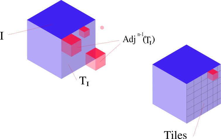
Figure 4. The red dyadic cubes constitute the family $\mathrm{Adj}^{n-1}.$

We order the cubes in ${\mathscr{C}}_{R}$ from the largest to the smallest one, and we label them as $I_{0},....,I_{N}$, for some $N\in\mathbb{N}$. This is true because the cardinality of ${\mathscr{C}}_{R}$ is finite (depending on $k_{0}$ - see Remarks 7.8 and 7.9). Let us start our construction with $I_{0}\in{\mathscr{C}}_{R}$ (thus $I_{0}$ is the largest cube in ${\mathscr{C}}_{R}$). We look at one of its $(n-1)$-dimensional faces, let us denote it by $T_{I_{0}}$. Now, let $I$ be a cube of minimal side length contained in $\mathrm{Adj}^{n-1}(T_{I_{0}})$; let $n(I)\in\mathbb{N}$ be such that $\ell(I)=2^{-n(I)}$. We consider the family of cubes in $\Delta_{n(I)}$ such that they have an $(n-1)$-dimensional face contained in $T_{I_{0}}$. We call this family $\Delta_{n(I)}(T_{I_{0}})$. Let us denote by

$${\mathscr{D}}^{n-1}(T_{I_{0}})$$ (7.21)

the family of $(n-1)$-dimensional faces of the same side length of $I$, such that they are both an $(n-1)$-dimensional face of a cube $J\in\Delta_{n(I)}(T_{I_{0}})$ and also they are contained in $T_{I_{0}}$. We may refer to this family as the tiles of $T_{I_{0}}$. We repeat the same procedure for $I_{1},...,I_{N}$; we don’t do anything if $\mathrm{Adj}^{n-1}(T_{I_{j}})=\emptyset$ for some face $T_{I_{j}}$ of $I_{j}$, $1\leq j\leq N$. Note that the definition of $\mathrm{Adj}^{n-1}(T_{I})$ imposes the following: if two cubes $I$ and $I^{\prime}$ are so that, say, $\ell(I)>\ell(I^{\prime})$ and $I^{\prime}\in\mathrm{Adj}^{n-1}(T_{I})$, then the tiles constructed on $T_{I}$ will be the same one that we have on the face $T_{I^{\prime}}\subset T_{I}$. The construction of tiles on the other $(n-1)$-faces of $I^{\prime}$ will not change the ones already present in $T_{I^{\prime}}$. This procedure terminates since ${\mathscr{C}}_{R}$ is finite.

Once we constructed $(n-1)$-dimensional tiles on all the $(n-1)$-dimensional faces of all cubes in ${\mathscr{C}}_{R}$, we rest. After, we proceed as follows. Denote by

$${\mathscr{F}}^{n-1}$$ (7.22)

the family of $(n-1)$-dimensional faces belonging to some cube in ${\mathscr{C}}_{R}$. If $T\in{\mathscr{F}}^{n-1}$ and ${\mathscr{D}}^{n-1}(T)\neq\emptyset$, the put the elements of ${\mathscr{D}}^{n-1}(T)$ in ${\mathscr{F}}^{n-1}$ and take $T$ away. If ${\mathscr{D}}^{n-1}(T)=\emptyset$, then leave $T$ in ${\mathscr{F}}^{n-1}$. Next, we repeat the previous construction: order the elements of ${\mathscr{F}}^{n-1}$ in decreasing order with respect to side length and consider $T_{0}$ (the largest face in ${\mathscr{F}}^{n-1}$). For each $(n-2)$-dimensional face $F_{T_{0}}$ of $T_{0}$ we set

$$\mathrm{Adj}^{n-2}(F_{T_{0}})$$

$$:=\left\{T\in{\mathscr{F}}^{n-1}\,|\,\ell(T)<\ell(T_{0}),\,T\cap F_{T_{0}}\mbox{ is an }(n-2)-\mbox{face of }T\mbox{ and }T\cap F_{T_{0}}\subset\mathop{\mathrm{missing}}{Int}(F_{T_{0}})\right\}.$$

We now look for the minimal element of $\mathrm{Adj}^{n-2}(F_{T_{0}})$, and call it $T$. Let $n(T)\in\mathbb{Z}$ so that $\ell(T)=2^{n(T)}$; we now tessellate $F_{T_{0}}$ with tiles of side length $2^{n(T)}$; by tessellate here we mean the obvious thing, i.e. we substitute $F_{T_{0}}$ with its children of size $2^{n(T)}$. Let us denote the tiles so constructed by

$${\mathscr{D}}^{n-2}(F_{T_{0}}).$$

We repeat the same procedure for $T_{1},...,T_{N^{\prime}}\in{\mathscr{F}}^{n-1}$. Again, the construction of $(n-2)$-dimensional tiles for smaller $(n-2)$-dimensional faces does not affect the previously constructed tiles for larger faces. This procedure terminates since ${\mathscr{F}}^{n-1}$ is finite, which follows trivially from ${\mathscr{C}}_{R}$ being finite. Next, we set

$${\mathscr{F}}^{n-2}$$

to be the family of $(n-2)$-dimensional faces coming from elements of ${\mathscr{F}}^{n-1}$, and we immediately modify it as above: if ${\mathscr{D}}^{n-2}(F_{T})\neq\emptyset$, for $T\in{\mathscr{F}}^{n-1}$, we substitute $F_{T}$ with the corresponding family of tiles.

We continue this construction: we obtain ${\mathscr{F}}^{n-3}$ from ${\mathscr{F}}^{n-2}$, ${\mathscr{F}}^{n-4}$ from ${\mathscr{F}}^{n-3}$, and so on, until we construct ${\mathscr{F}}^{d}$. We stop at this point and we set (see Figure 5).

$$E_{R}:=\widetilde{E}_{R}\cup\left(\bigcup_{F\in{\mathscr{F}}^{d}}F\right).$$ (7.23)

Lemma 7.14.

The set $E_{R}$ is Ahlfors $d$-regular.

Proof.

Lower regularity follows immediately from the definition and the lower regularity of $\widetilde{E}_{R}$. On the other hand, note that for any cube $I\in{\mathscr{C}}_{R}$, any smaller neighbouring cube $I^{\prime}\in{\mathscr{C}}_{R}$ will satisfy $\ell(I^{\prime})>\tau\ell(I)$ (using Lemma 7.11, (2)). If we envelope $I$ in cubes of side length $\ell(I)\tau$ and we consider the $d$-dimensional skeleton of this family of cubes, we see that the overall additional mass will not exceed a constant times $\ell(I)^{d}$, where such a constant depends on $n$, $d$ and $\tau$. Thus upper regularity is also preserved. ∎

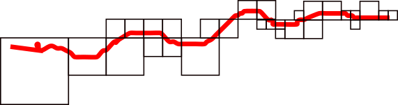
Figure 5. The approximating set $E_{R}$.

Notation 7.15.

From now on, we fix the notation for the regularity constant of $E_{R}$: it will be denoted by $\mathsf{C}_{3}$ and depends on $n,d,\tau$ anf the regularity constant of $\widetilde{E}_{R}$.

8. A topological condition on approximating skeleta

We now introduce a condition on $E_{R}$ which will imply the existence of a uniformly rectifiable sets lying close to it. This is akin to the condition David calls TND (topological nondegeneracy condition) in [Dav04]. We modified it somewhat to adhere to our trees structure. Let $R\in\mathsf{Top}(k_{0})$ and $E_{R}$ be the set constructed in Section 7.2, i.e. the set given in (7.23).

Definition 8.1 (STC).

Let $C_{2}$ be an arbitrary big constant and let $k_{0}\in\mathbb{N}$ be as in the statement of Lemma 7.7. Let $E$ be a lower content ($\mathsf{c}_{1},d)$-regular set. Then we say that the family of subsets $\{E_{R}\}_{R\in\mathsf{Top}(k_{0})}$ satisfies the skeletal topological condition with parameter $C_{2}$, or $C_{2}$-(STC), if we can find positive constants

$$0<\alpha_{1},\,\eta_{1},\,\delta_{1}<1\mbox{ and }r_{1}>0$$ (8.1)

such that

$$\mbox{for all }x_{1}\in E,$$ (8.2)

$$\mbox{for all }R\in\mathsf{Top}(k_{0})\mbox{ s.t. }x_{1}\in R\mbox{ and }\frac{\ell(R)}{4}\leq r_{1},$$ (8.3)

$$\mbox{for all }Q\in\mathsf{Tree}(R)\mbox{ s.t. }x_{1}\in Q,$$ (8.4)

for which

$$\mathcal{H}^{d}\left(E_{R}\cap B(x_{1},\ell(Q))\right)\leq C_{2}\ell(Q)^{d}$$ (8.5)

holds, there is a ball $B(x_{2},r_{2})$ centered on $E$ and contained in $B(x_{1},\ell(Q))$ such that, for each one-parameter family $\{\varphi_{t}\}_{0\leq t\leq 1}$ of Lipschitz functions on $\mathbb{R}^{n}$ that satisfy (3.10), (3.11), (3.12) and

$$\mathop{\mathrm{missing}}{dist}(\varphi_{t}(y),E)\leq\alpha_{1}\ell(Q)\mbox{ for }t\in[0,1]\mbox{ and }y\in E_{R}\cap B(x_{2},r_{2}),$$ (8.6)

we have that

$$\mathcal{H}^{d}\left(\varphi_{1}(E_{R}\cap B(x_{2},r_{2}))\right)\geq\delta_{1}\ell(Q)^{d}+\mathcal{H}^{d}(E_{R}\cap A_{\eta_{1}\ell(Q)}(x_{2},r_{2})),$$ (8.7)

where

$$A_{\eta_{1}\ell(Q)}(x_{2},r_{2}):=B(x_{2},r_{2})\setminus B(x_{2},r_{2}-\eta_{1}\ell(Q)).$$ (8.8)

Remark 8.2.

Note that

$$r_{2}>\eta_{1}\ell(Q);$$ (8.9)

if $r_{2}\leq\eta_{1}\ell(Q)$, then $A_{\eta_{1}\ell(Q)}=B(x_{2},r_{2})$. Thus if we apply (8.7) with $\varphi_{t}(y)=y$, then we would obtain that $\mathcal{H}^{d}(E_{R}\cap B(x_{2},r_{2}))>\mathcal{H}^{d}(E_{R}\cap B(x_{2},r_{2}))$, a contradiction.

9. Federer-Fleming projections

In this section we will construct a Federer-Fleming projection of $E$ onto a subset of $E_{R}$; we will use these projections in the next section to prove that the topological condition (TC) on $E$ implies the condition STC on the approximating skeleta. Our construction will mimic the one in [Dav04], which in turn comes from [DS00]. The difference here is that we are dealing with a skeleton of faces coming from cubes of different sizes.

9.1. Preliminaries and notation

9.1.1. The story so far.

Let $E$ be the stable $d$-surface that we started with. From Lemma 7.2 we know that it is lower content ($d,\mathsf{c}_{1}$)-regular. Hence we apply the coronisation as described in Subsection 7.2 (Lemma 7.7), which is a collection of ‘top cubes’ $\{R\}_{R\in\mathsf{Top}(k_{0})}$. For each such an $R$ we construct an approximating set which we called $\widetilde{E}_{R}$ (see its definition in (7.20), and see recall the definition of ${\mathscr{C}}_{R}$ in (7.19)). We subsequently modify it as in (7.23).

9.1.2. Some notation

Now fix any (Christ-David) ‘top cube’ $R\subset E$ and let $B(x,r)$ be a ball centered on it (the construction below will be applied to the ball $B(x_{2},r_{2})$ as in the definition of STC, Definition 8.1). Set

$${\mathscr{C}}_{R}(x,r):=\left\{I\in{\mathscr{C}}_{R}\,|\,I\cap B(x,r)\neq\emptyset\right\};$$ (9.1)

$${\mathscr{F}}^{m}(x,r):=\left\{T\in{\mathscr{F}}^{m}\,|\,T\cap B(x,r)\neq\emptyset\right\}\mbox{ for }d\leq m\leq n-1;$$ (9.2)

$$D_{R}(x,r):=\bigcup_{I\in{\mathscr{C}}_{R}(x,r)}I.$$ (9.3)

We define a further family, which we call ${\mathscr{C}}_{R}^{2}(x,r)$, as follows:

• First we add to ${\mathscr{C}}_{R}^{2}(x,r)$ all the dyadic cubes belonging to ${\mathscr{C}}_{R}(x,r)$ (so in particular ${\mathscr{C}}_{R}(x,r)$ will be a subfamily of ${\mathscr{C}}^{2}_{R}(x,r)$.

• Next, consider the collection (which we call) ${\mathscr{F}}(x,r)$ of dyadic cubes $J\in\Delta\setminus{\mathscr{C}}_{R}$ so that

  $$\mathop{\mathrm{missing}}{Int}(J)\subset\left(\bigcup_{I\in{\mathscr{C}}_{R}(x,r)}I\right)^{c};$$ (9.4)

  $$\mbox{ there exists a dyadic cube }I\in{\mathscr{C}}_{R}(x,r)\mbox{ s.t. }I\cap J\neq\emptyset;$$ (9.5)

  $$\min\left\{\ell(I)\,|\,I\in{\mathcal{N}}(J)\right\}\leq\ell(J)\leq\max\left\{\ell(I)\,|\,I\in{\mathcal{N}}(J)\right\},$$ (9.6)

  where ${\mathcal{N}}(J)$ is the family of cubes in ${\mathscr{C}}_{R}(x,r)$ which intersects $J$. Then we add to ${\mathscr{C}}_{R}^{2}(x,r)$ the subcollection of maximal dyadic cubes (see Definition 2.3) of ${\mathscr{F}}(x,r)$.

The family ${\mathscr{C}}^{2}_{R}(x,r)\setminus{\mathscr{C}}_{R}(x,r)$ forms a sheath for ${\mathscr{C}}_{R}(x,r)$ (imagine the plastic covering of some Minecraft electrical wires). Finally we define

$$D_{R}^{2}(x,r):=\bigcup_{I\in{\mathscr{C}}_{R}^{2}(x,r)}I.$$ (9.7)

9.2. The construction

Once again, recall the definition of $E_{R}$ as in (7.23). The following lemma is similar to Proposition 3.1 in [DS00], and so is the proof. The only difference is that we are working with a non-uniform grid of cubes.

Lemma 9.1.

Let $E\subset\mathbb{R}^{n}$ be a lower content ($d,\mathsf{c}_{1}$)-regular subset with $\mathcal{H}^{d}(E)<+\infty$. Given $(x,r)\in E\times\mathbb{R}_{+}$, there exists a Lipschitz map $\pi:\mathbb{R}^{n}\to\mathbb{R}^{n}$ such that

$$\pi(y)=y\mbox{ whenever }x\in\mathbb{R}^{n}\setminus D_{R}^{2}(x,r);$$ (9.8)

$$\pi(I)\subset I\mbox{ if }I\in{\mathscr{C}}_{R}^{2}(x,r);$$ (9.9)

$$\pi(E)\cap I\subset E_{R}\cap I\mbox{ for any }I\in{\mathscr{C}}_{R}(x,r).$$ (9.10)

We will obtain our Federer-Fleming projection as the composition of a finite number of maps which we will define inductively. We start by defining a map, let us call it $\pi_{1}$, that will send points in $D_{R}^{2}(x,r)\cap E$ into $(n-1)$-dimensional faces. We define $\pi_{1}$ on each individual cube $I\in{\mathscr{C}}_{R}^{2}(x,r)$ as follows. Pick a point $c_{I}\in I$ such that $c_{I}\notin E$. This is possible since $\mathcal{H}^{d}(E)<\infty$ (recall (7.3)) and thus, in particular, $\mathop{\mathrm{missing}}{dim}_{H}(E)<d+1$; a standard argument then shows that $E$ is porous, and thus such a point $c_{I}$ must exist. Then for $y\in E\cap\mathop{\mathrm{missing}}{Int}(I)$, we set

$$\pi_{1}(y)\mbox{ to be the point where the line passing through }y\mbox{ and }c_{I}\mbox{ meets }\partial I;$$ (9.11)

note that, then, $\pi_{1}(y)$ belong to some $(n-1)$ dimensional face of $I$. On the other hand, if $y\in E\cap\partial I$, we set

$$\pi_{1}(y)=y.$$ (9.12)

We then

$$\mbox{extend }\pi_{1}\mbox{ on the whole of }I\mbox{ such that }\pi_{1}(I)\subset I\mbox{ and }\pi_{1}\mbox{ is Lipschitz on }I.$$ (9.13)

(This can be done via standard extension results, see for example [Hei05, Theorem 2.5]). Note that this definition is coherent, in the sense that one can glue together the definition of $\pi_{1}$ on each $I\in{\mathscr{C}}_{R}^{2}(x,r)$ into a unique map $\pi_{1}$ defined on the whole of $D^{2}_{R}(x,r)$. Indeed, if $I,I^{\prime}\in{\mathscr{C}}_{R}^{2}(x,r)$ are so that $I\cap I^{\prime}\neq\emptyset$, then the definition of $\pi_{1}$ on $I^{\prime}\cap I$ must agree, since $I\cap I^{\prime}$ is contained in $\partial I$ and $\partial I^{\prime}$. Furthermore, we extend the definition of $\pi_{1}$ to $\mathbb{R}^{n}\setminus D_{R}^{2}(x,r)$ by setting

$$\pi_{1}(y)=y$$ (9.14)

there. Thus (9.11)-(9.14) give a coherent definition of $\pi_{1}$ on the whole of $\mathbb{R}^{n}$.

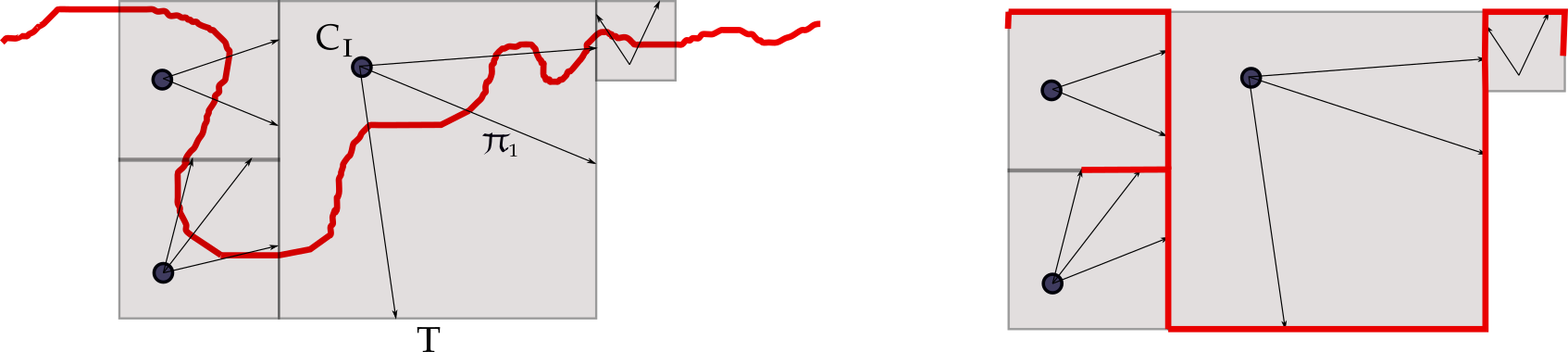
Figure 6. An image to give an heuristic idea of Federer-Fleming projections onto skeleta.

Now, if $d=n-1$, we stop here and we set $\varphi:=\pi_{1}$. Otherwise, we continue as follows. We want to send points on the $(n-1)$-dimensional faces of cubes in ${\mathscr{C}}_{R}(x,r)$ to the boundaries of these faces, which are, in turn, $(n-2)$-dimensional faces. To do this, we proceed, as above, by defining the map we need on each individual face. Recall the definition of ${\mathscr{F}}^{n-1}$ in (7.22). Let us start by defining $\pi_{2}$ on each $\partial T\cup(\pi_{1}(E)\cap T)$, where $T\in{\mathscr{F}}^{n-1}$: we repeat the construction above. Namely,

$$\mbox{we find a point }c_{T}\in\mathop{\mathrm{missing}}{Int}(T)\setminus\pi_{1}(E)\mbox{ and then project radially }\pi_{1}(E)\cap T\mbox{ onto }\partial T;$$ (9.15)

once again, this definition leave unchanged those points which already belong to $\partial T$. Moreover, we can extend $\pi_{2}$ as a Lipschitz map from $T$ to $T$ (for each $T\in{\mathscr{F}}^{n-1}$), again by standard extension results. In this way, we obtain a coherently defined map on $\partial I$, for each $I\in{\mathscr{C}}_{R}(x,r)$. Next,

$$\mbox{we extend }\pi_{2}\mbox{ to the whole of }D_{R}(x,r)\mbox{ by requiring that }$$

$$\pi_{2}(I)\subset I\mbox{ for any }I\in{\mathscr{C}}_{R}(x,r).$$ (9.16)

To do so, we want to extend $\pi_{2}$ from $\partial I$, to the whole of $I$, with the requirement that $\pi_{2}(I)\subset I$. Let $c_{I}$ be the center of $I$. We set $\pi_{2}(c_{I}):=x^{*}$, where $x^{*}$ is any point in $\pi_{2}(\partial I)$. Then for any point $y\in\partial I$, and a point $x=tc_{I}+(1-t)y$, $t\in[0,1]$, (so that $x$ belongs to the line segment from $c_{I}$ to $y$), we set

$$\pi_{2}(x)=t\pi_{2}(c_{I})+(1-t)\pi_{2}(y).$$

Note that, because both $\pi_{2}(c_{I})$ and $\pi_{2}(y)$ belong to $\partial I$, and $I$ is convex, then $\pi_{2}(x)\in I$. Let us check that $\pi_{2}$ so defined is Lipschitz on $I$. Take any two points $x_{1},x_{2}\in I$ and write them as

$$x_{1}=tc_{I}+(1-t)y_{1},\,\,t\in[0,1]\mbox{ and }y_{1}\in\partial I;$$ (9.17)

$$x_{2}=sc_{I}+(1-s)y_{2},\,\,s\in[0,1]\mbox{ and }y_{2}\in\partial I.$$ (9.18)

Assume first that $t=s$. We can assume that $t=s<1$, for otherwise $x_{1}=x_{2}$. In this case, we have that

$$|\pi_{2}(x_{1})-\pi_{2}(x_{2})|=|(1-t)(\pi_{2}(y_{1})-\pi_{2}(y_{2}))| \leq|1-t|C|y_{1}-y_{2}|$$

$$=C\,|(1-t)(y_{1}-y_{2})|$$

$$=|x_{1}-x_{2}|.$$

Here the constant $C$ is the Lipschitz constant of $\pi_{2}$ as function defined on $\partial I$. Next, let us suppose that for $x_{1}$ and $x_{2}$ as in (9.17) and (9.18), we have that $y_{1}=y_{2}$, hence they lie on the same line segment from $c_{I}$ to $\partial I$. We first note that (assuming without loss of generality that $t>s$),

$$|x_{1}-x_{2}|=|(t-s)(c_{I}-y_{1})|\geq(t-s)\ell(I).$$

On the other hand, simply beacuse both $\pi_{2}(c_{I})$ and $\pi_{2}(y_{1})$ belong to $\partial I$, we have that

$$|\pi_{2}(x_{1})-\pi_{2}(x_{2})|=|(t-s)(\pi_{2}(c_{I})-\pi_{2}(y_{1}))|\leq\sqrt{n}\,(t-s)\ell(I).$$

Thus $|\pi_{2}(x_{1})-\pi_{2}(x_{2})|\leq\sqrt{n}|x_{1}-x_{2}|$. Finally, for any two points $x_{1},x_{2}\in I$ as in (9.17) and (9.18), put

$$x_{2}^{\prime}:=t\,c_{I}+(1-t)y_{2}.$$

Note that there exists a constant, depending only on $n$, so that

$$|x_{2}-x_{2}^{\prime}|\leq C\,|x_{1}-x_{2}|,$$ (9.19)

But then, by the triangle inequality, we also have that

$$|x_{1}-x_{2}^{\prime}|\leq(C+1)|x_{1}-x_{2}|.$$

This give us the following:

$$|\pi_{2}(x_{1})-\pi_{2}(x_{2})| \leq|\pi_{2}(x_{1})-\pi_{2}(x_{2}^{\prime})|+|\pi_{2}(x_{2}^{\prime})-\pi_{2}(x_{2})|$$

$$\leq C\left(|x_{1}-x_{2}^{\prime}|+|x_{2}^{\prime}-x_{2}|\right)$$

$$\leq C^{\prime}|x_{1}-x_{2}|.$$

This proves that the extension of $\pi_{2}$ to the whole of $I$ is indeed Lipschitz, with a Lipschitz constant comparable to that of $\pi_{2}$ as defined on $\partial I$. Now we let $\pi_{2}$ on $D(x,r)$ to be piecewise defined on each $I$ of ${\mathscr{C}}_{R}(x,r)$.

Let us see why this definition is coherent. If $T,T^{\prime}\in{\mathscr{F}}^{n-1}$, $T\cap T^{\prime}\neq\emptyset$ and let us assume without loss of generality that $\ell(T^{\prime})<\ell(T)$, then either

$$T^{\prime}\subset T,$$ (9.20)

or

$$T\cap T^{\prime}\subset\left(\partial T\right)\cup\left(\partial T^{\prime}\right).$$ (9.21)

If (9.21) holds, than we immediately see that the definition of $\pi_{2}$ is coherent, since we defined to be the identity on both $\partial T$ and $\partial T^{\prime}$. We divert a moment from the main construction to show that the former case does not happen.

Lemma 9.2.

The case (9.20) does not occur.

Proof.

Let $T\in{\mathscr{F}}^{n-1}(x,r)$, and assume first that $T$ is an $(n-1)$-dimensional face (as opposed to a tile) of a cube $I\in{\mathscr{C}}_{R}(x,r)$. Suppose that there exists an element $T^{\prime}$ of ${\mathscr{F}}^{n-1}(x,r)$ such that $T^{\prime}\subset T$. If $T^{\prime}$ is an $(n-1)$-dimensional face of a cube $I^{\prime}\in{\mathscr{C}}_{R}(x,r)$, then, by construction of ${\mathscr{F}}^{n-1}(x,r)$, we must have that $I^{\prime}\in\mathrm{Adj}^{n-1}(T)$. But then $F$ cannot possibly belong to ${\mathscr{F}}^{n-1}$. On the other hand, if $T^{\prime}$ is a tile, then also in this case $T$ cannot be in ${\mathscr{F}}^{n-1}$, since it should have been tessellated into tiles of the same size of $T^{\prime}$.

Suppose now that $T$ is a tile itself. But by construction, we cannot have two tiles of different sizes lying on the same $(n-1)$-dimensional face. Thus $T^{\prime}\subset T$ has to really be $T^{\prime}=T$, which contradicts the fact that $\ell(T^{\prime})<\ell(T)$. ∎

Thus the definition of $\pi_{2}$ is coherent. Let us now define $\pi_{2}$ on those $(n-1)$-dimensional faces $T^{\prime}$ of cubes in ${\mathscr{C}}_{R}^{2}(x,r)$ such that $\mathop{\mathrm{missing}}{Int}(T^{\prime})\nsubseteq\mathop{\mathrm{missing}}{Int}(D_{R}(x,r))$ (recall the definition of $D_{R}(x,r)$, (9.3)). These are the faces which form the external boundary of the sheath ${\mathscr{C}}_{R}^{2}(x,r)\setminus{\mathscr{C}}_{R}(x,r)$. For these faces we leave everything unchanged, i.e. we let

$$\pi_{2}(y)=y \mbox{ for any }y\in T,$$ (9.22)

$$\mbox{ where }T\mbox{ is a }(n-1)\mbox{-dimensional face }T\mbox{ with }T\nsubseteq D_{R}(x,r).$$ (9.23)

Finally, we extend $\pi_{2}$ to the whole of $D^{2}_{R}(x,r)\setminus D_{R}(x,r)$ by requiring that

$$\pi_{2}(I)\subset I\mbox{ for }I\in{\mathscr{C}}^{2}_{R}(x,r)\setminus{\mathscr{C}}_{R}(x,r)$$

$$\pi_{2}(y)=y\mbox{ whenever }y\in\partial D_{R}^{2}(x,r).$$ (9.24)

(This can be done in the same fashion as for (9.2)). We finally set

$$\pi_{2}(y)=y\mbox{ whenever }y\in\mathbb{R}^{n}\setminus D_{R}^{2}(x,r).$$ (9.25)

Hence (9.15)-(9.25) give us a Lipschitz map $\pi_{2}$ defined on the whole of $\mathbb{R}^{n}$. Now, if $d=n-2$, then we can set $\varphi=\pi_{2}\circ\pi_{1}$, otherwise we continue projecting. To do so, we define a third map $\pi_{3}$. We follow the procedure above: first, if $F$ is an $(n-2)$-dimensional element of ${\mathscr{F}}^{n-2}(x,r)$, then we set $\pi_{3}$ to be the radial projection from some point $c_{F}\in\mathop{\mathrm{missing}}{Int}(F)\setminus\pi_{2}\circ\pi_{1}(E)$ defined on $\partial F\cup\left(\pi_{1}\circ\pi_{2}(E)\cap F\right)$. In particular, $\pi_{3}(y)=y$ if $y\in\partial F$. Next, we extend $\pi_{3}$ to the whole of $T$, by requiring that $\pi_{3}(T)\subset T$; if there is an element $F$ of ${\mathscr{F}}^{n-2}$ such that $(\pi_{2}\circ\pi_{1})(E)\cap F=\emptyset$, we set $\pi_{3}(y)=y$ on such an element. Note that this definition is coherent by construction of ${\mathscr{F}}^{n-2}(x,r)$, as in the definition of $\pi_{2}$. Next, we extend the definition of $\pi_{3}$ to the faces $T$ of dimension $(n-1)$, requiring that for any such a face, we have $\pi_{3}(T)\subset T$ and $\pi_{3}(\mathop{\mathrm{missing}}{Int}(T))\subset\mathop{\mathrm{missing}}{Int}(T)$; we also require that $\pi_{3}(y)=y$ on those faces $T$ such that $T\cap D_{R}(x,r)=\emptyset$. Finally, we extend $\pi_{3}$ to the whole cubes $I$, requiring again that $\pi_{3}(I)\subset I$. At this point, note that for $y\in E$, we have

• either $\pi_{3}\circ\pi_{2}\circ\pi_{1}(y)\in\mathbb{R}^{n}\setminus D^{2}_{R}(x,r)$ if $y\in E\setminus D^{2}_{R}(x,r)$;

• or $\pi_{3}\circ\pi_{2}\circ\pi_{1}(y)\in T$, where $T$ is a $(n-1)$-dimensional face of a cube in ${\mathscr{C}}_{R}^{2}(x,r)\mbox{ s.t. }T\nsubseteq D_{R}(x,r)$;

• or $\pi_{3}\circ\pi_{2}\circ\pi_{1}(y)\in F$, where $F\in{\mathscr{F}}^{n-3}$.

Remark 9.3.

The second possibility only occurs for those $y\in E$ so that

$$y\in\bigcup_{I\in{\mathscr{C}}^{2}(x,r)\setminus{\mathscr{C}}(x,r)}I\subset\mathbb{R}^{n}\setminus B(x,r).$$

We continue constructing projections in this fashion until reaching the $d$-dimensional skeleton. At each step, we construct $\pi_{m}$, for $n-d\leq m\leq n$, first on the elements of ${\mathscr{F}}^{m}(x,r)$ as a radial projection, and second we extend this definition to faces (or tiles) of increasing dimension, asking (if $F^{\prime}$ represents on such face or tile) that $\pi_{m}(F^{\prime})\subset F^{\prime}$. We stop once $\pi_{n-d}$ has been defined. If $y\in E$, then, setting

$$\pi:=\pi_{n-d}\circ\cdots\circ\pi_{1},$$ (9.26)

we see that

• either $\pi(y)\in\mathbb{R}^{n}\setminus D_{R}^{2}(x,r)$, if $y\in E\setminus D^{2}_{R}(x,r);$

• or $\pi(y)\in T$, where $T$ is an $(n-1)$-dimensional face of a cube in ${\mathscr{C}}_{R}^{2}(x,r)$ such that $T\nsubseteq D_{R}(x,r)$;

• or $\pi(y)\in F$, where $F\in{\mathscr{F}}^{d}(x,r)$.

Note that the definition of $\pi$ is coherent for the same reasons that $\pi_{3}$ and $\pi_{2}$ were coherent. In particular, $\pi$ is Lipschitz (with possible a very large Lipschitz constant, but we do not mind this). Moreover, it follows from the construction that the properties (9.8), (9.9) and (9.10) are satisfied; this concludes the proof of Lemma 9.1

10. Topological stability of $E$ implies topological stability of the approximating set

In this section, we will prove that if $E$ is a stable $d$-surface (i.e. it satisfies condition (TC)) and if we approximate it with sets $E_{R}$ (as in (7.23)), then these sets satisfy the skeletal topological condition STC (see Definition 8.1).

10.0.1. The story so far.

Let $E$ be the stable $d$-surface that we started with. From Lemma 7.2 we know that it is lower content ($d,\mathsf{c}_{1}$)-regular. Hence we apply the coronisation as described in Subsection 7.2 (Lemma 7.7), which is a collection of ‘top cubes’ $\{R\}_{R\in\mathsf{Top}(k_{0})}$. For each such an $R$ we construct an approximating set which we called $\widetilde{E}_{R}$ (see its definition in (7.20), and see recall the definition of ${\mathscr{C}}_{R}$ in (7.19)). We subsequently modify it as in (7.23). Next we defined coherent Federer-Fleming projections (Lemma 9.1), through which one can map $E$ into $E_{R}$ in a Lipschtitz continuous way (without control on the Lipschitz constant).

The idea behind the proof of the Lemma 10.1 below is that by composing the Federer-Fleming projection (which maps $E$ into $E_{R}$) with a deformation $\varphi_{t}$ as in the definition of the skeletal topological condition (Def. 8.1), we obtain an allowed Lipschitz deformation for $E$ (see Def. 3.4). Consequently we obtain a lower bound for the $d$-measure of the deformation of $E$ (as in (TC)), and, because $E_{R}$ lies close to $E$, we obtain a lower bound for the measure of the deformation of $E_{R}$ (as in (8.7)). See Figure 7.

Figure 7. The topological condition on $E$ implies the skeletal topological condition on $E_{R}$: composing $\pi$ with $\varphi_{1}$ gives an allowed deformation for $E$.

Lemma 10.1.

Let $E\subset\mathbb{R}^{n}$ be such that $0<\mathcal{H}^{d}(E)<\infty$. Suppose also that $E$ is a stable $d$-surface with constants $(r_{0},\alpha_{0},\delta_{0},\eta_{0},\gamma_{0})$; let $Q_{0}\in\mathcal{D}(E)$ be such that $\ell(Q_{0})<r_{0}$. For some $k_{0}\in\mathbb{N}$, apply Lemma 7.7 to $Q_{0}$ to obtain a corona decomposition $\mathsf{Top}(k_{0})=\mathsf{Top}(Q_{0},k_{0})$ and a family of sets $\{E_{R}\}_{R\in\mathsf{Top}(k_{0})}$ with parameter $\tau$. Then we can find parameters $r_{1},\alpha_{1},\delta_{1}$ and $\eta_{1}$, so that the family $\{E_{R}\}_{R\in\mathsf{Top}(k_{0})}$ satisfies the $C_{2}$-(STC) for $C_{2}$ sufficiently large.

We will prove this lemma through a few lemmas below. Set

$$\tau<\frac{1}{1000}\min\{\alpha_{0},\eta_{0}\}.$$ (10.1)

To ease the notation we let $\mathsf{Top}=\mathsf{Top}(k_{0})$; recall that for a large constant $C_{2}$, we want to prove the existence of parameters $r_{1}>0$ and $0<\alpha_{1},\delta_{1}<1$ (as in (8.1)) so that for all $x_{1}\in E$, $R\in\mathsf{Top}$ and $Q\in\mathsf{Tree}(R)$ with $x_{1}\in Q$, as in (8.2)-(8.3), for which (8.5) holds, we have the lower bound (8.7). Let us immediately choose the parameters in (8.1) (our choice is somewhat similar to that of [Dav04], equation 3.10, except that we have one extra parameter to deal with, since our topological condition is weaker). We set

$$r_{1}=r_{0},\mbox{ where }r_{0}\mbox{ is the one given by }\eqref{e:TC};$$ (10.2)

$$\alpha_{1}=C\min(\eta_{0},\alpha_{0});$$ (10.3)

$$\eta_{1}=C\frac{c(\eta_{0})\delta_{0}\gamma_{0}}{C_{2}},\mbox{ where }c(\eta_{0}):=\frac{\eta_{0}^{2}}{1+\eta_{0}};$$ (10.4)

$$\delta_{1}=C\delta_{0}.$$ (10.5)

We will fix the various absolute constants $C$ as we go along. They will only depend on $n$. Let $x_{1}$, $R$ and $Q$ as in (8.2), (8.3) and (8.4). We now want to find a ball $B(x_{2},r_{2})$ with the required properties: recall that the topological condition in Definition 3.5 gives us a ball $B=B(x_{B},r_{B})$ centered on $E$ (satisfying (3.21) and (3.20)) where the lower bounds (TC) holds. We choose

$$x_{2}=x_{B}\mbox{ and }$$ (10.6)

$$r_{2}\mbox{ s.t. }\frac{r(B)}{1+\eta_{0}}\leq r_{2}\leq(1-\eta_{0})r(B).$$ (10.7)

Remark 10.2.

We would also like the quantity $\mathcal{H}^{d}\left(E_{R}\cap A_{\eta_{1}\ell(Q)}(x_{2},r_{2})\right)$ to be small. Indeed, if for some choice of $r_{2}$ it held that

$$\mathcal{H}^{d}\left(E_{R}\cap A_{\eta_{1}\ell(Q)}(x_{2},r_{2})\right)\lesssim\delta_{1}\ell(Q)^{d},$$ (10.8)

then in order to verify (8.7) (adjusting the constant in the definition of $\delta_{1}$), we would only have to check that

$$\mathcal{H}^{d}\left(\varphi_{1}(E_{R}\cap B(x_{2},r_{2}))\right)\geq\delta_{1}\ell(Q)^{d}.$$ (10.9)

Claim 10.3.

There exists a radius $r_{2}$ satisfying (10.7) and (10.8).

Proof.

Choose $C$ in (10.4) so that

$$C\delta_{0}/C_{2}=10^{-1}.$$ (10.10)

Then we consider ten radii $\{s_{k}\}_{k=0}^{9}$ given as

$$s_{k}=\frac{r(B)}{1+\eta_{0}}-\frac{k}{10}c(\eta_{0})r(B),\quad 0\leq k\leq 9.$$

Note that each $s_{k}$ satisfies (10.7). Since

$$\eta_{1}\ell(Q)\stackrel{{\scriptstyle\eqref{e:eta}}}{{=}}C\frac{c(\eta_{0})\gamma_{0}\delta_{0}}{C_{2}}\ell(Q)\stackrel{{\scriptstyle\eqref{e:r_B}}}{{\leq}}\frac{C\delta_{0}}{C_{2}}c(\eta_{0})r(B)\stackrel{{\scriptstyle\eqref{e:TND-C-eta}}}{{\leq}}\frac{1}{10}c(\eta_{0})r(B),$$

the annuli $\left\{A_{\eta_{1}\ell(Q)}(x_{2},s_{k})\right\}_{k=0}^{9}$ are pairwise disjoint. Then we see that

$$\sum_{k=0}^{9}\mathcal{H}^{d}(E_{R}\cap A_{\eta_{1}\ell(Q)}(x_{2},s_{k}))\leq\mathcal{H}^{d}\left(E_{R}\cap B(x_{2},r(B))\right)\stackrel{{\scriptstyle\eqref{e:TND-upper}}}{{\leq}}C_{2}\ell(Q)^{d}.$$

Then by the pigeonhole principle and (10.4) and (10.5), we must have that for some $0\leq k\leq 9$,

$$\mathcal{H}^{d}(E_{R}\cap A_{\eta_{1}\ell(Q)}(x_{2},s_{k}))\leq 10^{-1}C_{2}\ell(Q)^{d}\stackrel{{\scriptstyle\eqref{e:TND-C-eta}}}{{\lesssim}}C\delta_{0}\ell(Q)^{d}\stackrel{{\scriptstyle\eqref{e:delta}}}{{\approx}}\delta_{1}\ell(Q)^{d}.$$

Thus (10.8) holds putting $r_{2}=s_{k}$. ∎

Lemma 10.4.

Let $I\in{\mathscr{C}}_{R}(x_{2},r_{2})$, where ${\mathscr{C}}_{R}(x,r)$ is defined in (9.1); also, here $x_{2}=x_{1}\in Q$, for some $Q\in\mathsf{Tree}(R)$, and $r_{2}$ is as in (10.7). Then

$$\ell(I)\leq C\,\tau\,\ell(Q).$$ (10.11)

Proof.

It suffices to prove the lemma for $Q\in\mathsf{Stop}(R)$, since if $Q\in\mathsf{Tree}(R)\setminus\mathsf{Stop}(R)$, then there exists a cube $Q^{\prime}\in\mathsf{Stop}(R)$ with $x_{2}=x_{1}\in Q^{\prime}$ and $\ell(Q^{\prime})<\ell(Q)$. If $I\in{\mathscr{C}}_{R}$, then we know that $\ell(I)\lesssim\tau d_{R}(I)$ (recall that $\tau$ depends on $\alpha_{0}$ and $\eta_{0}$ and was fixed in (10.1)). Moreover, $d_{R}(\cdot)$ is 1-Lipschitz. Then if $y\in I\cap B(x_{2},r_{2})$, we have that

$$d_{R}(I)\leq d_{R}(y)\leq|y-x_{2}|+d_{R}(x_{2}).$$

Because $r_{2}\approx\ell(Q)$, $|x_{2}-y|\leq\ell(Q)$. On the other hand, we see that

$$d_{R}(x_{2})=\inf_{P\in\mathsf{Stop}(R)}\left(\ell(P)+\mathop{\mathrm{missing}}{dist}(x_{2},P)\right)\leq\ell(Q).$$

∎

Remark 10.5.

Note that the same holds for any $I\in{\mathscr{C}}_{R}^{2}(x_{2},r_{2})$, by definition of ${\mathscr{C}}_{R}^{2}(x_{2},r_{2})$ (as defined in (9.4), (9.5) and (9.6)).

Lemma 10.6.

Let $(x_{2},r_{2})$ to be as chosen in (10.6) and (10.7). For any one parameter family of Lipschitz deformations $\left\{\varphi_{t}\right\}_{0\leq t\leq 1}$ satisfying (3.10), (3.11), (3.12) and (8.6) (relative to $(x_{2},r_{2})$), the property (10.9) holds, that is, we have

$$\mathcal{H}^{d}(\varphi_{1}(E_{R}\cap B(x_{2},r_{2})))\geq\delta_{1}\ell(Q)^{d}.$$

Proof.

We have two ingredients we want to put together to achieve (10.9): on one hand, we know that something similar holds for $E$ (i.e. TC); on the other hand, we know that $E$ is locally well approximated by $E_{R}$, and we have a continuous (actually Lipschitz) way to move from $E$ to $E_{R}$ (i.e. the Federer-Fleming projection we constructed in the previous section). The idea is therefore the following: pick the one parameter family $\varphi_{t}$ for which we want to show (10.9), and pick $\pi$ as in Lemma 9.1. We will construct from these a deformation $f$ which satisfies conditions (3.10)-(3.13); hence from (TC), we will deduce (10.9).

Set

$$\pi_{t}(y):=t\,\pi(y)+(1-t)\,y.$$

If $y\in D_{R}^{2}(x_{2},r_{2})$, let $I\in{\mathscr{C}}_{R}^{2}(x_{2},r_{2})$ be the dyadic cube containing $y$ (recall the definition of ${\mathscr{C}}_{R}^{2}(x_{2},r_{2})$ in (9.4)-(9.6)); then (9.9) tells us that

$$|\pi_{t}(y)-y|\leq t|\pi(y)-y|\leq n^{1/2}\ell(I)$$

if $\pi_{t}$ actually moves $y$. Otherwise this quantity is equal to zero (this happens for example if $I\in{\mathscr{C}}_{R}^{2}(x_{2},r_{2})\setminus{\mathscr{C}}_{R}(x_{2},r_{2})$). By Lemma 10.4 we have that

$$\ell(I)\lesssim\tau d_{R}(y)\leq\tau\left(|y-x_{2}|+d_{R}(x_{2})\right)\lesssim\tau\ell(Q).$$

Hence we obtain

$$|\pi(y)-y|\lesssim\tau\ell(Q)\mbox{ for all }y\in\mathbb{R}^{n}.$$ (10.12)

Let us now define $\{f_{t}\}_{0\leq t\leq 1}$. We set

$$f_{t}(y):=\begin{cases}\pi_{2t}(y)&\mbox{ if }0\leq t\leq\frac{1}{2};\\ \varphi_{2t-1}(\pi(y))&\mbox{ if }\frac{1}{2}\leq t\leq 1.\end{cases}$$ (10.13)

We claim that $\{f_{t}\}$ satisfies the conditions (3.10)-(3.13) applied to the larger ball

$$B(x_{2},\widetilde{r})\mbox{ where }\widetilde{r}:=(1+\eta_{0})r_{2}.$$ (10.14)

See Figure 8. We verify these conditions one by one. It is immediate from the definition that each $f_{t}$ is Lipschitz.

Figure 8. The set-up for the proof of Lemma 10.6

.

Claim 10.7.

We have that $f_{t}(\overline{B}(x,\widetilde{r}))\subset\overline{B}(x,\widetilde{r})$, i.e. (3.10) holds for $f_{t}$.

Proof of claim 10.7.

Note that

$$B(x_{2},r_{2})\cap E\subset D_{R}(x_{2},r_{2})\subset D_{R}^{2}(x_{2},r_{2}),$$ (10.15)

where $D_{R}(x_{2},r_{2})$ and $D^{2}_{R}(x_{2},r_{2})$ were defined in (9.3) and (9.7); (10.15) follows immediately from the definitions. Moreover, using Lemma 10.4, we see that any cube which was added to ${\mathscr{C}}_{R}^{2}(x_{2},r_{2})\setminus{\mathscr{C}}_{R}(x_{2},r_{2})$, must have side length at most $C\tau\ell(Q)$ (recall that $Q$ satisfies (8.4) and $x_{2}$ and $r_{2}$ are as in (10.6) and (10.7), respectively). Thus $D_{R}^{2}(x_{2},r_{2})\subset B(x_{2},r_{2}+C\tau\ell(Q))$ and also, since

$$\tau\ell(Q)\stackrel{{\scriptstyle\eqref{e:tau}}}{{\leq}}\frac{1}{100}\eta_{0}\ell(Q)\stackrel{{\scriptstyle\eqref{e:TND-r_2}}}{{\leq}}\eta_{0}r_{2},$$

we have that

$$D^{2}_{R}(x_{2},r_{2})\subset B(x_{2},r_{2}+\tau\ell(Q))\subset B(x_{2},(1+\eta_{0})r_{2})\subset B(x_{2},\widetilde{r}).$$ (10.16)

Let us consider a few cases separately.

• If $y\in D^{2}_{R}(x_{2},r_{2})$, then $\pi_{t}(y)\in D^{2}_{R}(x_{2},r_{2})$ for all $0\leq t\leq 1$ (by Lemma 9.1), and so

  $$f_{s}(y)\in B(x_{2},\widetilde{r})\mbox{ for }s\leq\frac{1}{2}\mbox{ whenever }y\in D_{R}^{2}(x_{2},r_{2}).$$

  Now, recall that (3.10) holds for $\varphi_{t}$ (relative to $B(x_{2},r_{2})$); hence if, together with $y\in D_{R}^{2}(x_{2},r_{2})$, we also have that $\pi(y)\in\overline{B}(x_{2},r_{2})$, we then conclude that $f_{s}(y)\in\overline{B}(x_{2},r_{2})$ for $\frac{1}{2}\leq s\leq 1$. Also (3.12) holds for $\varphi_{t}$: if $\pi(y)\notin\overline{B}(x_{2},r_{2})$, then, for $\frac{1}{2}\leq s\leq 1$ and recalling (10.15), $f_{s}(y)=\pi(y)\in D_{R}^{2}(x_{2},r_{2})$. We obtain then that

  $$f_{s}(y)\in B(x_{2},\widetilde{r})\mbox{ whenever }y\in D_{R}^{2}(x_{2},r_{2}).$$ (10.17)

• Suppose now that $y\in B(x_{2},\widetilde{r})\setminus D_{R}^{2}(x_{2},r_{2})$; by construction $\pi(y)=y$ whenever $y\in\mathbb{R}^{n}\setminus D_{R}^{2}(x_{2},r_{2})$, hence $\pi_{t}(y)=y$ for $t\in[0,1]$, and thus

  $$f_{s}(y)=y\mbox{ for }s\leq\frac{1}{2}\mbox{ whenever }y\in B(x_{2},\widetilde{r})\setminus D_{R}^{2}(x_{2},r_{2}).$$ (10.18)

  But because $\varphi_{t}$ satisfies (3.12) relative to $B(x_{2},r_{2})$ (that is, $\varphi_{t}$ is the identity outside $B(x_{2},r_{2})$, and becuase $B(x_{2},r_{2})\subset D^{2}_{R}(x_{2},r_{2})$ (i.e. (10.15)), then $\varphi_{t}(\pi(y))=\pi(y)=y$. Thus we obtain that

  $$f_{s}(y)\in B(x_{2},\widetilde{r})\mbox{ for }\frac{1}{2}\leq s\leq 1\mbox{ whenever }y\in B(x_{2},\widetilde{r})\setminus D_{R}^{2}(x_{2},r_{2}).$$ (10.19)

  Now (10.17), (10.18) and (10.19) give us the property (3.10) for $\{f_{s}\}$ relative to $B(x_{2},\widetilde{r})$.

∎

Claim 10.8.

The path $s\mapsto f_{s}(y)$ is continuous, that is, (3.11) holds for $f_{t}$. Condition (3.12) also holds.

Proof of claim 10.8.

The first conclusion is clear, since $t\mapsto\pi_{t}(y)$ is continuous; moreover, $\pi_{1}(y)=\pi(y)=\varphi_{0}(\pi(y))=f_{\frac{1}{2}}(y)$, and $t\mapsto\varphi_{2t-1}(\pi(y))$ is also continuous. As for the second conclusion of the claim, we see that $f_{0}(y)=\pi_{0}(y)=y$; if $y\in\mathbb{R}^{n}\setminus B(x_{2},\widetilde{r})$, we have seen above that $f_{t}(y)=y$. Thus (3.12) holds for $\{f_{s}\}$ in $B(x_{2},\widetilde{r})$. ∎

Claim 10.9.

Condition (3.13) holds, i.e. we have that $\mathop{\mathrm{missing}}{dist}(f_{s}(y),E)\leq\alpha_{0}\widetilde{r}$ for $s\in[0,1]$ and $y\in E\cap B(x_{2},\widetilde{r})$.

Proof of claim 10.9.

First, consider $0\leq s\leq\frac{1}{2}$; let $y\in E\cap B(x_{2},\widetilde{r})$; then we have

$$\mathop{\mathrm{missing}}{dist}(f_{s}(y),E)=\mathop{\mathrm{missing}}{dist}(\pi_{2s}(y),E)\leq|\pi_{2s}(y)-y|$$

$$\stackrel{{\scriptstyle\eqref{e:TP-TNDg}}}{{\leq}}n^{\frac{1}{2}}\tau\ell(Q)\stackrel{{\scriptstyle\eqref{e:tau}}}{{\leq}}\frac{1}{3}\alpha_{0}\ell(Q)\stackrel{{\scriptstyle\eqref{e:TND-r_2},\eqref{e:TND-wt-r}}}{{\leq}}\alpha_{0}\widetilde{r}.$$

Now suppose that $s>\frac{1}{2}$. If $y\in B(x_{2},\widetilde{r})\cap E$, then,

$$\mbox{either }y\in D_{R}^{2}(x_{2},r_{2})$$ (10.20)

$$\mbox{or }y\notin D^{2}_{R}(x_{2},r_{2}).$$ (10.21)

If $y$ is so that (10.21) holds, then $\pi(y)=y$, and moreover, from (3.12) for $\varphi_{t}$ relative to $B(x_{2},r_{2})$, we see that $\varphi_{2s-1}(\pi(y))=\varphi_{2s-1}(y)=y$. Hence (3.13) holds in this case. On the other hand, suppose that (10.20) holds. Then from the proof of Lemma 9.1, we have that

$$\mbox{either }\pi(y)\in E_{R},$$ (10.22)

$$\mbox{or }\pi(y)\in T,\mbox{ where }T\mbox{ is an }(n-1)\mbox{-face with }T\nsubseteq D_{R}(x_{2},r_{2}).$$ (10.23)

If (10.22) holds, then $\mathop{\mathrm{missing}}{dist}(\varphi_{2s-1}(\pi(y),E)\leq\alpha_{1}\ell(Q)$ by (8.6) applied to $\varphi_{t}$; this immediately implies $\mathop{\mathrm{missing}}{dist}(f_{s}(y),E)\leq\alpha_{0}\widetilde{r}$ for $s>\frac{1}{2}$ by the choice of $\alpha_{1}$ in (10.3). On the other hand, if (10.23) holds, we must have $\pi(y)\notin B(x_{2},r_{2})$ (by construction of $\pi$), and therefore $\varphi_{2s-1}(\pi(y))=\pi(y)$. Now $\pi(y)$ belongs to a cube in ${\mathscr{C}}_{R}^{2}(x_{2},r_{2})$ with side length at most $\tau\ell(Q)$ and touching $E$, hence we retrieve $\mathop{\mathrm{missing}}{dist}(f_{s}(y),E)\leq\alpha_{0}\ell(Q)\leq\alpha_{0}\widetilde{r}$. Together with the previous estimates, we obtain that $\{f_{s}\}$ satisfies (3.13) for all $s\in[0,1]$. This concludes the proof of claim 10.9. ∎

Claims 10.7-10.9 show that $\{f_{t}\}$ is an allowed Lipschtiz deformation relative to the ball $B(x_{2},\widetilde{r})$, with $\widetilde{r}=(1+\eta_{0})r_{2}$. Since $B(x_{2},\widetilde{r}_{2})\subset B$, this in particular implies that $\{f_{t}\}$ is an allowed Lipschitz deformation for $B$ (the ‘stable’ ball satisfying (3.19), (3.20), (3.21)). Hence since we assumed that $E$ is a stable $d$-surface, we apply (TC), and obtain

$$\mathcal{H}^{d}\left(B(x_{B},(1-\eta_{0})r(B))\cap f_{1}(E)\right)\geq\delta_{0}\ell(Q)^{d}.$$ (10.24)

But recall that $r_{2}\geq(1-\eta_{0})r(B)$ and thus $B(x_{2},r_{2})\supset B(x_{2},(1-\eta_{0})\widetilde{r})$. Then,

$$\mathcal{H}^{d}\left(B(x_{2},r_{2})\cap f_{1}(E)\right)\stackrel{{\scriptstyle\eqref{e:TP-TNDo}}}{{\geq}}\mathcal{H}^{d}\left(B(x_{B},(1-\eta_{0})r(B))\cap f_{1}(E)\right)\geq\delta_{0}\ell(Q)^{d}.$$ (10.25)

Recall from above that if $y\in E$ and it is such that $y\notin D_{R}(x_{2},r_{2})$, then $f_{1}(y)\notin B(x_{2},r_{2})$. Thus,

$$B(x_{2},r_{2})\cap f_{1}(E)\subset f_{1}(D_{R}(x_{2},r_{2})\cap E).$$

Note also that $\pi(E\cap D_{R}(x_{2},r_{2}))\subset E_{R}$. Thus we obtain, using (10.25), (10.8) and (10.5),

$$\mathcal{H}^{d}\left(\varphi_{1}(E_{R})\cap B(x_{2},r_{2})\right)\geq 2\delta_{1}\ell(Q)^{d}.$$

This concludes the proof of Lemma 10.6. ∎

Proof of Lemma 10.1.

Recall from Remark 10.2, that proving the estimates (10.8) and (10.9) is enough to prove (8.7), and thus Lemma 10.1. Claim 10.3 gives the first estimate, while Lemma 10.6 gives the second one. ∎

11. A further approximating set

We now construct a dyadic approximation of $E_{R}$ (this is for technical reasons which will become transparent later on). We will also then show that this approximation satisfies the STC.

Let $\rho$ be a small parameter (which we will fix later, and can be assumed to be of the form $2^{-k},k\in\mathbb{N}$). We write

$$\Delta_{\rho}:=\Delta_{j(\rho)},$$

where $j(\rho)$ is an integer so that $2^{-j(\rho)}=\rho.$ We set

$${\mathscr{C}}_{R,\rho}:=\left\{I\in\Delta_{\rho}\,|\,I\cap E_{R}\neq\emptyset\right\};$$ (11.1)

$$E_{\rho}=E_{R,\rho}:=\bigcup_{I\in{\mathscr{C}}_{R,\rho}}\partial_{d}I.$$ (11.2)

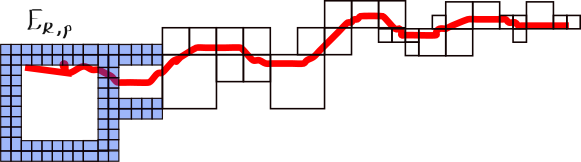
Figure 9. The red set represents $E$; the black squares represent $E_{R}$, while the blue smaller ones represent $E_{R,\rho}$.

Lemma 11.1.

Let $I_{*}$ be the smallest cube in ${\mathscr{C}}_{R}$ (which exists since ${\mathscr{C}}_{R}$ is finite). Then for all $\rho<\ell(I_{*})$, $E_{R,\rho}$ is Ahlfors regular, with regularity constant comparable to that of $E_{R}$.

Proof.

Let $T$ be a $d$-dimensional face of some cube $J\in{\mathscr{C}}_{R}$. Denote by ${\mathscr{F}}^{d}_{\rho}$ the collection of $d$-dimensional faces from cubes in ${\mathscr{C}}_{R,\rho}$. Then we can cover $T$ with a subcollection of ${\mathscr{F}}^{d}_{\rho}$ with pairwise disjoint interiors. If we denote such a collection by ${\mathscr{F}}^{d}_{\rho}(T)$, then it is obvious that

$$\mathcal{H}^{d}(T)=\sum_{F\in{\mathscr{F}}^{d}_{\rho}}\mathcal{H}^{d}(F).$$

To each such a face $F\in{\mathscr{F}}^{d}_{\rho}$, there corresponds a bounded number of cubes so that $F\subset I\in{\mathscr{C}}_{R,\rho}$. This bounded number depends only on $n$ and $d$. Moreover, each of these cubes has a bounded number of other $d$-dimensional faces, and, again, this number depends only on $n$ and $d$. Thus, if we denote by $\Delta_{\rho}(T)$ the family of cubes in $\Delta_{\rho}$ which also meet $T$, we see that

$$\sum_{I\in\Delta_{\rho}(T)}\mathcal{H}^{d}(I)\leq C(n,d)\sum_{F\in{\mathscr{F}}^{d}_{\rho}}\mathcal{H}^{d}(F)=C(n,d)\,\mathcal{H}^{d}(T).$$

Then, we see that

$$\mathcal{H}^{d}\left(E_{R,\rho}\cap B(x,r)\right) \leq\sum_{\begin{subarray}{c}I\in{\mathscr{C}}_{R,\rho}\\ I\cap B(x,r)\neq\emptyset\end{subarray}}\mathcal{H}^{d}(\partial_{d}I)$$

$$\leq\sum_{J\in{\mathscr{C}}_{R}(x,r)}\sum_{T\,\text{face of }J}\sum_{I\in{\mathscr{F}}^{d}_{\rho}(T)}\mathcal{H}^{d}(\partial_{d}I)$$

$$\leq C(n,d)\sum_{J\in{\mathscr{C}}_{R}(x,r)}\mathcal{H}^{d}(\partial_{d}J)$$

$$\lesssim\mathsf{C}_{3}r^{d}.$$

Recall that $\mathsf{C}_{3}$ is the upper regularity constant of $E_{R}$ (see Notation 7.15). By enlarging it if necessary, we will assume that $\mathsf{C}_{3}$ is also the regularity constant of $E_{R,\rho}$.

It is immediate to conclude lower regularity for those points in $E_{R,\rho}\cap E_{R}$. Hence let $x\in E_{R,\rho}\setminus E_{R}$. If $r$ is comparable to $\rho$ or smaller, than clearly $\mathcal{H}^{d}(B(x,r)\cap E_{R,\rho})\gtrsim r^{d}$ since $E_{R,\rho}$ is just a $d$-dimensional affine plane at this scale. If $r\gtrsim\rho$, then, by construction, $B(x,r)$ will contain a ball $B^{\prime}$ with $r(B^{\prime})\approx r$ and such that $B^{\prime}$ is centered on $E_{R}$. We then use the lower regularity of $E_{R}$ to conclude that $E_{R,\rho}$ is lower $d$-regular, too. ∎

Remark 11.2.

By making it even larger if needed, we assume that $\mathsf{C}_{3}$ is the Ahlfors $d$-regularity constant of $E_{R,\rho}$; it will not be useful to distinguish the Ahlfors regularity constants of $E_{R}$ and $E_{R,\rho}$; we will call them both $\mathsf{C}_{3}$.

Lemma 11.3.

Lemma 10.1 holds when we substitute $E_{R}$ with $E_{R,\rho}$.

In other words, given a stable $d$-surface $E\subset\mathbb{R}^{n}$ with constants ($r_{0},\alpha_{0},\delta_{0},\eta_{0}$) and with $0<\mathcal{H}^{d}(E)<+\infty$, let $Q_{0}\in\mathcal{D}(E)$ be so that $r_{0}<\ell(Q_{0})$. Then pick $k_{0}\in\mathbb{N}$ be sufficiently large so that we can construct the partition (with parameter $\tau>0$ as in (10.1)) $\mathsf{Top}(k_{0})$ of $\mathcal{D}(Q_{0},k_{0})$ as in Lemma 7.7. For each $R\in E_{R,\rho}$ and for $\rho>0$ to be fixed (see (11.3) below), we construct $E_{R,\rho}$ as described above. Then for $C_{2}$ sufficiently large, we can choose the parameters in the definition of STC (Definition 8.1) as in (10.2)-(10.5) and hence find a ball with center $x_{2}$ as in (10.6) and $r_{2}$ as in (10.7) so that $\mathcal{H}^{d}(E_{R,\rho}\cap B(x_{2},r_{2}))\geq\delta_{1}\ell(Q)^{d}+\mathcal{H}^{d}(E_{R,\rho}\cap A_{c\eta_{1}\ell(Q)}(x_{2},r_{2}))$, where $\varphi_{t}$ is a deformation as in Definition 8.1.

Proof.

Let $C_{2}$ be the same constant as in Lemma 10.1. We know from Section 10, that $E_{R}$ satisfies the STC with a choice of constants as in (10.2) - (10.5). Let $(x_{2},r_{2})$ as in (10.6) and (10.7). We now add to the constraint on $\rho$ given in the statement of Lemma 11.1, the following one: we ask that

$$\rho<\frac{1}{1000\sqrt{n}}\min\left\{\eta_{1},\alpha_{1}\right\}\ell(Q)\mbox{ for all $Q\in\mathsf{Tree}(R)$}.$$ (11.3)

Note that because $E_{R,\rho}$ is Ahlfors regular independently of $\rho$, this does not cause any trouble. Moreover, we can always choose $\rho>0$ since $\mathsf{Tree}(Q)$ is a finite family (recall Remark 7.8).

Let $Q\in\mathsf{Tree}(R)$ and $(x_{2},r_{2})$ as in the proof of Lemma 10.1, in particular see (10.6) and (10.7). Note that $E_{R,\rho}\cap B(x_{2},r_{2})\supset E_{R}\cap B(x_{2},r_{2})$, simply because $E_{R}\subset E_{R,\rho}$. Thus, also $\varphi_{1}(E_{R,\rho}\cap B(x_{2},r_{2}))\supset\varphi_{1}(E_{R}\cap B(x_{2},r_{2}))$, and therefore

$$\mathcal{H}^{d}(\varphi_{1}(E_{R,\rho}\cap B(x_{2},r_{2}))) \geq\mathcal{H}^{d}\left(\varphi_{1}(E_{R}\cap B(x_{2},r_{2}))\right)$$

$$\geq\delta_{1}\ell(Q)^{d}+\mathcal{H}^{d}(E_{R}\cap A_{\eta_{1}\ell(Q)}(x_{2},r_{2})).$$

But now note that if we choose a parameter $c>0$ sufficiently small, and we put $\widetilde{\eta}_{1}=c\eta_{1}$, then we see that

$$\mathcal{H}^{d}(E_{R}\cap A_{\eta_{1}\ell(Q)}(x_{2},r_{2}))\geq\mathcal{H}^{d}(E_{R,\rho}\cap A_{\widetilde{\eta}_{1}\ell(Q)}(x_{2},r_{2})).$$

Note that $c$ only depends on $n$ and $d$. Hence we obtain that

$$\mathcal{H}^{d}(\varphi_{1}(E_{R,\rho}\cap B(x_{2},r_{2})))\geq\delta_{1}\ell(Q)^{d}+\mathcal{H}^{d}(E_{R,\rho}\cap A_{\widetilde{\eta}_{1}\ell(Q)}(x_{2},r_{2})),$$ (11.4)

and the lemma is proven. ∎

Remark 11.4.

To ease the notation, we ignore the fact that we changed $\eta_{1}$ by a constant $c$, and we will continue denoting $\widetilde{\eta}_{1}$ by $\eta_{1}$.

12. A functional on skeleta

In this section, we show that the topological condition STC imposed on $E_{R}$ (and thus on $E_{R,\rho}$) tells us that $E_{R,\rho}$ has a large intersection (with repsect to the scale of each cube $Q\in\mathsf{Tree}(R)$) with a uniformly $d$-rectifiable set. The idea is to define a functional whose minimizer $F$ has large intersection with $E_{R,\rho}$. In turn $F$, by virtue of being a minimiser of such a functional, will turn out to be a quasiminimiser (in the sense of [DS00]), and thus uniformly rectifiable.

12.0.1. The story so far.

Let $E$ be the stable $d$-surface that we started with. From Lemma 7.2 we know that it is lower content ($d,\mathsf{c}_{1}$)-regular. Hence we apply the coronisation as described in Subsection 7.2 (Lemma 7.7), which is a collection of ‘top cubes’ $\{R\}_{R\in\mathsf{Top}(k_{0})}$. For each such an $R$ we construct an approximating set which we called $\widetilde{E}_{R}$ (see its definition in (7.20), and see recall the definition of ${\mathscr{C}}_{R}$ in (7.19)). We subsequently modify it as in (7.23). Next we defined coherent Federer-Fleming projections (Lemma 9.1), through which one can map $E$ into $E_{R}$ in a Lipschitz continuous way (without control on the Lipschitz constant). Via Federer-Fleming projections, we show that the fact that $E$ is a stable $d$-surface (with finite $d$-measure), implies that $E_{R}$, for each $R\in\mathsf{Top}(k_{0})$, is also topologically stable, in the sense of the skeletal topological condition in Definition 8.1; see Lemma 10.1. In Section 11 we construct, for technical reasons, a further approximating set $E_{R,\rho}$ (for each $R\in\mathsf{Top}(k_{0})$). Once again, the strategy below comes from [Dav04]. We adapt it to our current situation.

12.1. Definition of a functional $J$.

12.1.1. Preliminaries

Let $C_{2}$ be a large constant (depending on $\mathsf{C}_{3}$, the Ahlfors regularity constant of $E_{R,\rho}$ and $E_{R}$) and $k_{0}$ a sufficiently large integer (as per Lemma 7.7). Then STC gives us constants $r_{1}<r_{0}$, and $0<\alpha_{1},\eta_{1},\delta_{1}<1$ (as in (8.1)) such that for every choice of $x_{1}\in E$, $R\in\mathsf{Top}(k_{0})$ and $Q\in\mathsf{Tree}(R)$ as in (8.2), (8.3) and (8.4) respectively, with also $\mathcal{H}^{d}(E_{R}\cap B(x_{1},\ell(Q)))\leq C_{2}\ell(Q)^{d}$, we can find a ball $B(x_{2},r_{2})\subset B(x_{1},\ell(Q))$ centered on $E$ for which, given an appropriate one-parameter family of Lipschitz deformations $\{\varphi_{t}\}$, we have the lower bound (8.7). From the previous sections, we see that this holds for both $E_{R}$ and $E_{R,\rho}$.

Fix a cube $Q\in\mathsf{Tree}(R)$ and let $(x_{2},r_{2})$ be as in (10.6) and (10.7). To simplify the notation, we put

$$r:=r_{2};$$ (12.1)

$$x:=x_{2}.$$ (12.2)

For later use, let us set

$$B_{j}:=B\left(x,r-\eta_{1}\ell(Q)+\frac{j\eta_{1}\ell(Q)}{10}\right)\mbox{ for }0\leq j\leq 10.$$ (12.3)

Note that $B_{10}=B(x,r)$ and $B_{10}\setminus B_{0}=A_{\eta_{1}\ell(Q)}(x,r)$.

Recall the constraint on $\rho$, (11.3), and consider a constant $\sigma$ (let it be a power of $2$), so that

$$\frac{1}{200\sqrt{n}}\min\left\{\eta_{1},\alpha_{1}\right\}\ell(Q)\leq\sigma\leq\frac{1}{100\sqrt{n}}\min\left\{\eta_{1},\alpha_{1}\right\}\ell(Q).$$ (12.4)

Then we put

$$\Delta_{\sigma}(B_{6}):=\left\{I\in\Delta_{j(\sigma)}\,|\,I\cap B_{6}\neq\emptyset\right\};$$ (12.5)

$${\mathscr{C}}_{\sigma}^{1}(B_{6}):=\left\{I\in\Delta_{\sigma}(B_{6})\,|\,I\cap J\neq\emptyset\mbox{ for some }J\in{\mathscr{C}}_{R}\right\};$$ (12.6)

$${\mathscr{C}}_{\sigma}^{2}(B_{6}):=\left\{I\in\Delta_{\sigma}(B_{6})\,|\,\mbox{ there exists a }J\in{\mathscr{C}}_{\sigma}^{1}(B_{6})\mbox{ with }I\cap J\neq\emptyset\right\}.$$ (12.7)

Finally we put

$$V^{1}_{Q}:=\bigcup_{I\in{\mathscr{C}}^{1}_{\sigma}(B_{6})}I\enskip\enskip\mbox{ and}$$ (12.8)

$$V^{2}_{Q}:=\bigcup_{I\in{\mathscr{C}}^{2}_{\sigma}(B_{6})}I.$$ (12.9)

Note that for any cube $I\in{\mathscr{C}}_{R}(B_{6})$, there exists a cube $J\in{\mathscr{C}}_{\sigma}(B_{6})$ so that $J\supset I$.

Lemma 12.1.

With the notation above, we have that

$$B_{6}\cap E\subset V_{Q}^{2}\subset B_{7}\mbox{ and }$$ (12.10)

$$\mathop{\mathrm{missing}}{dist}(y,E)\leq\alpha_{1}\ell(Q)\mbox{ for all }y\in V^{1}_{Q}.$$ (12.11)

Proof.

The first inclusion in (12.10) is immediate. To see the second one, note that for any point $y\in V_{Q}^{2}$, we have that $\mathop{\mathrm{missing}}{dist}(y,V^{1}_{Q})\leq\sqrt{n}\sigma$. In turn, any point in $V^{1}_{Q}\setminus B_{6}$ can be at most $\sqrt{n}\sigma$ away from $\partial B_{6}$. Hence, by the choice of $\sigma$ in (12.4), we see that if $y\in V_{Q}^{2}\setminus B_{6}$, $\mathop{\mathrm{missing}}{dist}(y,\partial B_{6})<\frac{1}{10}\eta_{1}\ell(Q)$, and so (12.10) will be satisfied.

To prove (12.11), suppose first that $y\in V^{1}_{Q}$ is such that $y\in I$ for some $I\in{\mathscr{C}}_{R}$. Now, by construction, if $y\in V^{1}_{Q}$, then $y\in B(x_{2},r_{2})$, with $x_{2}\in Q$ and $r_{2}\approx\ell(Q)$. Thus $\mathop{\mathrm{missing}}{dist}(I,Q)\lesssim\ell(Q)$. This implies, using Lemma 7.11 (1), that

$$\ell(I)\leq\tau d_{R}(I)\leq\tau(\ell(Q)+\mathop{\mathrm{missing}}{dist}(I,Q))\lesssim\tau\ell(Q).$$

But recall also that $\tau\ll\alpha_{0},\eta_{0}$ (as in (10.1)), and thus also $\tau\ll\alpha_{1}$, by the choice of $\alpha_{1}$ in (10.3). Since $I\cap E\neq\emptyset$, for otherwise $I$ would not be in ${\mathscr{C}}_{R}$, we obtain that $\mathop{\mathrm{missing}}{dist}(y,E)\leq\alpha_{1}\ell(Q)$ for these $y$. Note that if $y\in V^{1}_{Q}$ but $y\notin I$ for all $I\in{\mathscr{C}}_{R}$, then by the way that $V^{1}_{Q}$ was defined, $\mathop{\mathrm{missing}}{dist}(y,I)<\sigma$ for some $I\in{\mathscr{C}}_{R}$. Keeping in mind the definition of $\sigma$ in (12.4), we can repeat the argument above to obtain (12.11) also in this case. ∎

12.1.2. The domain of the functional

We are now ready to fix the class of subsets upon which the said functional will be allowed to act. We set

$${\mathcal{F}}_{0}$$ (12.12)

to be the class of subsets $F$ of $\mathbb{R}^{n}$ such that

$$F\mbox{ is closed (in the topology of $\mathbb{R}^{n}$).}$$ (12.13)

$$F\subset V_{Q}^{2}$$ (12.14)

$$F=F^{*}\cup L.$$ (12.15)

Here $L$ denotes any subset of Hausdorff dimension smaller or equal than $d-1$; by $F^{*}$ we mean a finite union of $d$-dimensional faces of cubes coming from $\Delta_{\rho}$. We will call $F^{*}$ the coral part of $F$. In other words the class ${\mathcal{F}}_{0}$ is composed by subsets that are built out of a finite number of $d$-faces coming from cubes in $\Delta_{\rho}$. Let us consider a subclass of ${\mathcal{F}}_{0}$: we set

$${\mathcal{F}}:=\left\{F\in{\mathcal{F}}_{0}\,|\,F=\varphi_{1}(E_{R,\rho}\cap V_{Q}^{2})\right\},$$ (12.16)

where $\{\varphi_{t}\}_{0\leq t\leq 1}$ is a family of Lipschitz mappings on $\mathbb{R}^{n}$ such that

$$\varphi_{t}(V_{Q}^{2})\subset V_{Q}^{2}\mbox{ for all }t\in[0,1];$$ (12.17)

$$t\mapsto\varphi_{t}(y)\mbox{ is continuous for all }y\in\mathbb{R}^{n};$$ (12.18)

$$\varphi_{t}(y)=y\mbox{ for }t=0\mbox{ and for }y\in\mathbb{R}^{n}\setminus V_{Q}^{2};$$ (12.19)

$$\mathop{\mathrm{missing}}{dist}(\varphi_{t}(y),E_{R})<\alpha_{1}\ell(Q)\mbox{ for }y\in E_{R,\rho}\cap V_{Q}^{2}\mbox{ and all }t\in[0,1];$$ (12.20)

$$\varphi_{1}(y)\in V^{1}_{Q}\mbox{ for }y\in E_{R,\rho}\cap V_{Q}^{2}.$$ (12.21)

Lemma 12.2.

We have that $E_{R,\rho}\cap V_{Q}^{2}\in{\mathcal{F}}$. In particular, the class ${\mathcal{F}}$ is nonempty.

Proof.

We just take the trivial deformation $\varphi_{t}(y)=y$ for all $y$ and $t$, so that (12.17), (12.18) and (12.19) hold immediately. Moreover, by construction we have that all points in $E_{R,\rho}$ are contained in a cube from ${\mathscr{C}}_{R,\rho}$. The side length of these cubes is (much) less than $\alpha_{1}\ell(Q)$ and they must touch $E_{R}$. Hence $\mathop{\mathrm{missing}}{dist}(y,E_{R})<\alpha_{1}\ell(Q)$ and so (12.20) is satisfied. As far as condition (12.21) is concerned, we see that if $y\in E_{R,\rho}\cap V_{Q}^{2}$, then by definition of $E_{R,\rho}$ and ${\mathscr{C}}_{R,\rho}$ in (11.2) and (11.1), we see that $y$ must lies in a cube which belongs to ${\mathscr{C}}_{\sigma}^{1}(B_{6})$ (from the definition of $\sigma$ in (12.4)), and thus it must be in $V^{1}_{Q}$. ∎

We now define the aforementioned functional. For some $c_{2}<1$ to be chosen later, we put

$$M=\frac{\mathsf{C}_{3}}{c_{2}\,\delta_{1}},$$ (12.22)

where recall that $\mathsf{C}_{3}$ is the Ahlfors regularity constant of $E_{R}$ (as fixed in Notation 7.15) and of $E_{R,\rho}$. Then we set

$$J(F):=\mathcal{H}^{d}(F\cap E_{R,\rho})+M\,\mathcal{H}^{d}(F\setminus E_{R,\rho})\mbox{ for }F\in{\mathcal{F}}.$$ (12.23)

Note that $J(F)=J(F^{*})$ (with notation as in (12.15)), and there is only a finite number of sets like $F^{*}$. Thus there exists a set $\widetilde{F}\in{\mathcal{F}}$ such that

$$J(\widetilde{F})=\min_{F\in{\mathcal{F}}}J(F).$$

12.1.3. A minimiser of $J$ has large intersection with $E_{R,\rho}$

Note that, for a set $F\in{\mathcal{F}}$ trying to keep $J(F)$ small, it will be very expensive to have a large portion which does not intersect $E_{R,\rho}$, as $M$ can be quite large. This is the reason why we expect the minimiser $\widetilde{F}$ to have a large intersection with $E_{R,\rho}$. This also implies that a minimiser of $J$ also will lie close to $E_{R}$.

Lemma 12.3.

Let $\widetilde{F}$ be a minimiser of $J$ (as in (12.23)) in ${\mathcal{F}}$. Then

$$\mathcal{H}^{d}(E_{R,\rho}\cap\widetilde{F})\geq C\,\delta_{1}\ell(Q)^{d}.$$ (12.24)

Figure 10. The set up for the proof of Lemma 12.3: the grey and blue dyadic square are the ones with side length $\sigma$. The red dyadic square is from ${\mathscr{C}}_{R}$ (i.e. its skeleton forms part of $E_{R}$ - one should imagine red squares covering the black set; they were not drawn for simplicity). The small green squares are those whose skeleta form $E_{R,\rho}$.

Proof.

Because $\widetilde{F}\in{\mathcal{F}}$, then $\widetilde{F}=\varphi_{1}(E_{R,\rho}\cap V_{Q}^{2})$, where $\{\varphi_{t}\}$ satisfies (12.17)-(12.21). We want to check that this specific one parameter family $\varphi_{t}$ satisfies also the conditions for the deformations used for STC (see Definition 8.1) relative to $B(x,r)=B(x_{2},r_{2})$. Note that $\{\varphi_{t}\}$ satisfies (3.10), (3.11) and (3.12), since from (12.10), we have that $V_{Q}^{2}\subset B(x,r)$. We want to check that (8.6) hold, that is

$$\mathop{\mathrm{missing}}{dist}(\varphi_{t}(y),E_{R})\leq\frac{\alpha_{1}\ell(Q)}{2}\mbox{ for }t\in[0,1]\mbox{ and }y\in E_{R,\rho}\cap B(x,r).$$ (12.25)

So, let $y\in E_{R,\rho}\cap B(x,r)$. If $y\notin V_{Q}^{2}$, then $\varphi_{t}(y)=y$ by (12.19); since $y\in E_{R,\rho}$, then by construction $\mathop{\mathrm{missing}}{dist}(y,E_{R})<\sqrt{n}\rho\ll\alpha_{1}\ell(Q)$ (by the constraint on $\rho$ in (11.3)). Moreover, if $x\in E_{R}$ is the point closest to $y$, then $x\in\partial_{d}I$ for some $I\in{\mathscr{C}}_{R}(x,r)$ and, by Lemma 10.4, we have that $\ell(I)\lesssim\tau\ell(Q)$. All in all, this implies that $\mathop{\mathrm{missing}}{dist}(y,E)<\alpha_{1}\ell(Q)$ whenever $y\in B(x,r)\cap E_{R,\rho}$ does not belong to $V_{Q}^{2}$.

If $y\in V_{Q}^{2}\cap E_{R,\rho}$, then by (12.21), $\varphi_{t}(y)$ must lie in $V^{1}_{Q}$, and hence be at most $\sigma$ far away from $E_{R}$ (by construction); but $\sigma<\alpha_{1}\ell(Q)$, and repeating the argument of the previous case we again see that (12.25) holds.

Thus $\{\varphi_{t}\}$ is a one parameter family of Lipschitz deformations which satisfies the requirements stated in the definition of STC (see Definition 8.1). Recall that $E_{R,\rho}$ satisfies the STC (at scale $\ell(Q)$); we therefore have the lower bound (11.4), i.e.

$$\mathcal{H}^{d}(\varphi_{1}(E_{R,\rho}\cap B(x,r)))\geq\delta_{1}\ell(Q)^{d}+\mathcal{H}^{d}\left(E_{R,\rho}\cap A_{\widetilde{\eta}_{1}\ell(Q)}(x,r)\right).$$

Now, the family $\{\varphi_{t}\}$ which we are considering, not only satisfies (3.12), but also (12.19), and so, in particular,

$$\varphi_{1}\left(E_{R,\rho}\cap B(x,r)\right) =\varphi_{1}\left((V_{Q}^{2}\cap E_{R,\rho})\cup(E_{R,\rho}\cap(B(x,r)\setminus V_{Q}^{2}))\right)$$

$$=\varphi_{1}(E_{R,\rho}\cap V_{Q}^{2})\cup\left(E_{R,\rho}\cap(B(x,r)\setminus V_{Q}^{2})\right),$$

recalling that by definition (see (12.10)) $V_{Q}^{2}\subset B(x,r)$. Also, note that

$$E_{R,\rho}\cap(B(x,r)\setminus V_{Q}^{2})\subset A_{\widetilde{\eta}_{1}\ell(Q)}(x,r)\cap E_{R,\rho};$$ (12.26)

indeed, using $B_{6}\cap E_{R,\rho}\subset V_{Q}^{2}$, we see that $E_{R,\rho}\cap(B(x,r)\setminus V_{Q}^{2})\subset E_{R,\rho}\cap(B(x,r)\setminus B_{6})$, and (recalling the definition of the balls $B_{j}$’s (12.3)), $B(x,r)\setminus B_{6}\subset A_{\widetilde{\eta}_{1}\ell(Q)}(x,r)$. Thus we have

$$\mathcal{H}^{d}\left(\varphi_{1}(E_{R,\rho}\cap V_{Q}^{2})\right)+\mathcal{H}^{d}\left(A_{\widetilde{\eta}_{1}\ell(Q)}(x,r)\cap E_{R,\rho}\right)\geq\delta_{1}\ell(Q)^{d}+\mathcal{H}^{d}\left(E_{R,\rho}\cap A_{\widetilde{\eta}_{1}\ell(Q)}(x,r)\right)$$

and so

$$\mathcal{H}^{d}\left(\varphi_{1}(E_{R,\rho}\cap V_{Q}^{2})\right)\geq\delta_{1}\ell(Q)^{d}.$$ (12.27)

In particular, from the definition of ${\mathcal{F}}$, this inequality holds for any $F\in{\mathcal{F}}$. Recall now that we decided that $\widetilde{F}$ was a minimiser of $J$ (as defined in (12.23)). Thus we have that

$$J(\widetilde{F})\stackrel{{\scriptstyle\text{Lemma }\ref{l:dF}}}{{\leq}}J(E_{R,\rho}\cap V_{Q}^{2})=\mathcal{H}^{d}\left(E_{R,\rho}\cap V_{Q}^{2}\right)$$

$$\stackrel{{\scriptstyle\eqref{e:Ta}}}{{\leq}}\mathcal{H}^{d}\left(E_{R,\rho}\cap B(x,r)\right)\stackrel{{\scriptstyle\text{Lemma }\ref{l:Erho-ADR}}}{{\leq}}\mathsf{C}_{3}\ell(Q)^{d}.$$ (12.28)

Moreover, by definition of $J$,

$$\mathcal{H}^{d}\left(\widetilde{F}\setminus E_{R,\rho}\right)\leq\frac{J(\widetilde{F})}{M}\stackrel{{\scriptstyle\eqref{e:Jc}}}{{\leq}}\frac{C_{3}}{M}\ell(Q)^{d}\stackrel{{\scriptstyle\eqref{e:M}}}{{=}}c_{2}\,\delta_{1}\ell(Q)^{d}.$$ (12.29)

But then we have that, with $c_{2}$ sifficiently small,

$$\mathcal{H}^{d}\left(\widetilde{F}\cap E_{R,\rho}\right)=\mathcal{H}^{d}(\widetilde{F})-\mathcal{H}^{d}(\widetilde{F}\setminus E_{R,\rho})\stackrel{{\scriptstyle\eqref{e:Jb},\eqref{e:Jd}}}{{\geq}}\frac{\delta_{1}\ell(Q)^{d}}{2}.$$ (12.30)

This proves the Lemma. ∎

13. Almgren quasiminimality of $\widetilde{F}$.

Roughly speaking, a set $S$ in $\mathbb{R}^{n}$ is a (Almgren) quasiminimiser of the $d$-dimensional Hausdorff measure $\mathcal{H}^{d}$ if, whenever we deform $S$ in a suitable way, the $d$-measure of such deformations does not shrink too much. Quasiminimality is a form of stability: the set maintain its Hausdorff dimension under a suitable class of perturbations. Heuristically, this is the reason why we need to transfer the topological condition from $E$ to an Ahlfors regular set: in this case, modulo technicalities, quasimininality roughly coincides with our topological condition.

13.0.1. The story so far.

Let $E$ be the stable $d$-surface that we started with. From Lemma 7.2 we know that it is lower content ($d,\mathsf{c}_{1}$)-regular. Hence we apply the coronisation as described in Subsection 7.2 (Lemma 7.7), which is a collection of ‘top cubes’ $\{R\}_{R\in\mathsf{Top}(k_{0})}$. For each such an $R$ we construct an approximating set which we called $\widetilde{E}_{R}$ (see its definition in (7.20), and see recall the definition of ${\mathscr{C}}_{R}$ in (7.19)). We subsequently modify it as in (7.23). Next we defined coherent Federer-Fleming projections (Lemma 9.1), through which one can map $E$ into $E_{R}$ in a Lipschitz continuous way (without control on the Lipschitz constant). Via Federer-Fleming projections, we show that the fact that $E$ is a stable $d$-surface (with finite $d$-measure), implies that $E_{R}$, for each $R\in\mathsf{Top}(k_{0})$, is also topologically stable, in the sense of the skeletal topological condition in Definition 8.1; see Lemma 10.1. In Section 11 we construct, for technical reasons, a further approximating set $E_{R,\rho}$ (for each $R\in\mathsf{Top}(k_{0})$) which also satisfies the STC (Lemma 11.3). Then, it turns out that the minimiser $\widetilde{F}$ of the functional $J$, see (12.23), has large intersection with $E_{R,\rho}$ (Lemma 12.3).

13.1. Quasiminimizer sets for Hausdorff measure

We now recall from [DS00] the precise definitions to make this notion precise. Let $U$ be an open set in $\mathbb{R}^{n}$ and fix two constants

$$1\leq k<\infty\mbox{ and }0<\delta\leq+\infty.$$ (13.1)

Let $S\subset U$ be so that

$$S\neq\emptyset\mbox{ and }\overline{S}\setminus S\subset\mathbb{R}^{n}\setminus U.$$ (13.2)

Assume also that

$$\mathcal{H}^{d}(S\cap B)<+\infty\mbox{ for all balls }B\subset U.$$ (13.3)

Now, let us make precise what we mean by ‘deformations’ or ‘perturbations’. Given a set $S$, deformations of $S$ will be sets of the form $\phi(S)$, where

$$\phi:\mathbb{R}^{n}\to\mathbb{R}^{n}\mbox{ is Lipschitz }$$ (13.4)

and satisfies the following properties.

$$\operatorname{diam}\left(W\cup\phi(W)\right)\leq\delta\mbox{ where }W:=\left\{x\in\mathbb{R}^{n}\,|\,\phi(x)\neq x\right\};$$ (13.5)

$$\mathop{\mathrm{missing}}{dist}\left(W\cup\phi(W),\mathbb{R}^{n}\setminus U\right)>0;$$ (13.6)

$$\phi\mbox{ is Lipschitz-homotopic to the identity}.$$ (13.7)

The last requirement means that there exists a continuous map

$$h:\mathbb{R}^{n}\times[0,1]\to\mathbb{R}^{n}$$

such that $h(x,0)=x$ and $h(x,1)=\phi(x)$ for all $x\in\mathbb{R}^{n}$, such that $h(\cdot,t):\mathbb{R}^{n}\to\mathbb{R}^{n}$ is Lipschitz for all $t\in[0,1]$, and such that

$$\operatorname{diam}(\widehat{W})<\delta\mbox{ and }\mathop{\mathrm{missing}}{dist}(\widehat{W},\mathbb{R}^{n}\setminus U)>0,$$

where

$$\widehat{W}:=\bigcup_{t\in[0,1]}W_{t}\cup\phi_{t}(W_{t}),\enskip\phi_{t}(x)=h(x,t)\mbox{ and }W_{t}:=\left\{x\in\mathbb{R}^{n}\,|\,\phi_{t}(x)\neq x\right\}.$$

Definition 13.1.

Let $0<d<n$; let $U\subset\mathbb{R}^{n}$ be an open set and fix two constant $k,\delta$ as in (13.1). We say that $S\subset U$ is a $(U,k,\delta)$-quasiminimizer for $\mathcal{H}^{d}$ if $S$ satisfies (13.2), (13.3) and

$$\mathcal{H}^{d}(S\cap W)\leq k\mathcal{H}^{d}\left(\phi(S\cap W)\right)$$ (13.8)

for all Lipschitz mappings $\phi$ which satisfy (13.5), (13.6) and (13.7).

13.2. The set $\widetilde{F}$ is a quasiminimizer

This subsection is devoted to prove Lemma 13.2 below. Recall that $\widetilde{F}$ is a minimiser of the functional $J$ (as in (12.23)). Recall also the notation

$$B_{j}:=B\left(x,r-\eta_{1}\ell(Q)+\frac{j\eta_{1}\ell(Q)}{10}\right)\mbox{ for }0\leq j\leq 10,$$

where $x,r$ are as in (12.1), $\eta_{1}$ as in (10.4) (bearing in mind Remark 11.4) and $Q\in\mathsf{Tree}(R)$ as in (8.4).

Lemma 13.2.

The set

$$S:=\widetilde{F}\cap B_{2}$$ (13.9)

is a $(B_{2},k,\delta)$-quasiminimizer for $\mathcal{H}^{d}$, where

$$k=C\,4^{nd}M,$$ (13.10)

(here $C$ is a geometric constant), and

$$\delta=c_{3}\min\left\{\alpha_{1},\eta_{1}\right\}\ell(Q).$$ (13.11)

Here $0<c_{3}<1$ is a parameter bounded above by a universal constant.

We will need the following lemma from [Dav04]. We tailor it to our current notation.

Lemma 13.3 ([Dav04], Lemma 5.8).

Let $V^{1}$ be a finite union of dyadic cubes belonging to $\Delta_{\sigma}$, where $\sigma$ should be thought of as in (12.4). There exists a $4^{n}$-Lipschitz function $h$, defined on

$$V^{1}_{+}:=\left\{y\in\mathbb{R}^{n}\,|\,\mathop{\mathrm{missing}}{dist}(y,V^{1})\leq\frac{\sigma}{4}\right\}$$ (13.12)

and such that

$$h(V^{1}_{+})\subset V^{1}$$ (13.13)

$$h(y)=y\mbox{ for }y\in V^{1},$$ (13.14)

and

$$|h(y)-y|\leq n^{1/2}\sigma.$$ (13.15)

Recall that we want to show that $\widetilde{F}$ is a quasiminimal set for $\mathcal{H}^{d}$. Here is the idea to do so. We want to look at $\mathcal{H}^{d}(\phi(\widetilde{F}\cap W))$; what we know about $\widetilde{F}$ which makes us hope that it may well be a quasiminimal set is that $\widetilde{F}$ is a minimiser of the functional $J$ as defined in (12.23). We want to use this information. In other words, we would like to say that $\phi(\widetilde{F})$ is a competitor of $\widetilde{F}$ belonging to the class ${\mathcal{F}}$. Unfortunately, this is not true, in the sense that $\phi(\widetilde{F})$ may lie outside $V_{Q}^{1}$, and this is not permitted (see (12.21)). What we can do however, is first to retract $\phi(\widetilde{F})$ (which we will call $F_{1}$) back into $V_{Q}^{1}$ (using the map $h$ from Lemma 13.3); let us set $F_{2}:=h(F_{1})$. Next, we want to project $F_{2}$ onto some $d$-dimensional skeleton so that it belongs to ${\mathcal{F}}_{0}$ (as defined in (12.12)). This projection will happen in two steps, with two corresponding maps; we will denote the images so obtained by $F_{3}$ and then $F_{4}$; this latter one will be the needed competitor. The last step will be to show that these distortions of $\phi(\widetilde{F})$ don’t increase the size of $\phi(\widetilde{F})$ too much. In this way, first by the minimising property of $\widetilde{F}$ we will obtain a bound like $\mathcal{H}^{d}(\widetilde{F})\leq M\mathcal{H}^{d}(F_{4})$ and then, by this last step, a bound similar to $\mathcal{H}^{d}(F_{4})\leq C\mathcal{H}^{d}(\phi(\widetilde{F}))$ and thus establishing quasiminimality.

13.2.1. Construction of $F_{1}$ and $F_{2}$

Let us get started: we want to deform $\widetilde{F}$ with Lipshitz maps $\phi$ as in (13.4). Pick one such Lipshitz deformation $\phi$. We are interested in those points $y\in W\cap\widetilde{F}$, i.e. those points which are actually being moved by $\phi$. But by (13.5), we must have that $|\phi(y)-y|\leq\delta$. We put

$$\delta=c_{3}\min\left\{\alpha_{1},\eta_{1}\right\}\ell(Q),$$ (13.16)

where $c_{3}$ is a small parameter to be chosen soon. The rationale to choose $c_{3}$ is that we want $\phi(\widetilde{F})$ to lie in $V^{1}_{+}$, so that we may apply Lemma 13.3 and send $\phi(\widetilde{F})$ back into $V_{Q}^{1}$. Recall that $V^{1}_{+}$ is the set of points lying at most $\sigma/4$ far away from $V_{Q}^{1}$; recall also that $\widetilde{F}=\varphi_{1}(E_{\rho}\cap V^{2})\subset V_{Q}^{1}$ by (12.16) (the way ${\mathcal{F}}$ was defined) and the property of $\{\varphi_{t}\}$, (12.21). Hence for an appropriate choice of $c_{3}$, say

$$c_{3}=\frac{1}{300\sqrt{n}},$$ (13.17)

(see (12.4)) we have that if $y\in W\cap\widetilde{F}$, then

$$\phi(y)\in V^{1}_{+}.$$ (13.18)

We set

$$F_{1}:=\phi(\widetilde{F})\mbox{ and }$$ (13.19)

$$F_{2}:=h(F_{1})=h(\phi(\widetilde{F})).$$ (13.20)

In particular, $F_{2}\subset V_{Q}^{1}$ by Lemma 13.3.

13.2.2. Construction of $F_{3}$

We want to project $F_{2}$ back into a $d$-dimensional skeleton, since this is a requirement to belong to ${\mathcal{F}}_{0}$ (and so eventually to ${\mathcal{F}}$). By definition of ${\mathcal{F}}_{0}$, we will be projecting onto the $d$-skeleton of cubes coming from $\Delta_{\rho}$. We will use the following Lemma, which is taken from [DS00].

Lemma 13.4 (Lemma 11.14, [DS00]).

Let $j\in\mathbb{Z}$ and let $A$ be a compact subset of $\mathbb{R}^{n}$ such that $\mathcal{H}^{d}(A)<\infty$. Denote by $N(A)$ the union of all the cubes $I\in\Delta_{j}$ that touch a cube in $\Delta_{j}$ which intersects $A$. Then there is a Lipschitz mapping $f:\mathbb{R}^{n}\to\mathbb{R}^{n}$ with the following properties.

$$f(x)=x\mbox{ for }x\in\mathbb{R}^{n}\setminus N(A);$$ (13.21)

$$f(x)=x\mbox{ for all }x\in\mathcal{S}_{j,d};$$ (13.22)

$$f(A)\subset\mathcal{S}_{j,d};$$ (13.23)

$$f(I)\subset I\mbox{ for all }I\in\Delta_{j};$$ (13.24)

$$\mathcal{H}^{d}\left(f((A\cap I)\setminus{\mathcal{S}}_{j,d})\right)\leq C\,\mathcal{H}^{d}\left((A\cap I)\setminus{\mathcal{S}}_{j,d}\right)\mbox{ for all }I\in\Delta_{j}.$$ (13.25)

Recall the definition of ${\mathcal{S}}_{j,d}$ in (2.5).

We now apply Lemma 13.4 with

$$j=-j(\rho)\mbox{ and }A=F_{2}=h(\phi(\widetilde{F})),$$

and thus we set

$$F_{3}=f(F_{2})=(f\circ h\circ\phi)(\widetilde{F}).$$ (13.26)

Remark 13.5.

Let us note a couple of facts. First, we see that if $y\in\widetilde{F}\setminus W$, then $\phi(y)=y$ (by definition of $W$, as in (13.5)); but, still with the same $y$, also $h(\phi(y))=h(y)=y$, since $y\in V_{Q}^{1}$ already, and $h$ does not move such points (as in (13.14)), and further, $f(h(\phi(y)))=f(y)=y$ by (13.22), since $y\in\widetilde{F}$, and therefore it belongs to the $d$-face of some cubes from $\Delta_{\rho}$.

Lemma 13.6.

With the notation as above, we have

$$\mathop{\mathrm{missing}}{dim}\left(F_{3}\setminus{\mathcal{S}}_{-j(\rho),d}\right)\leq d-1.$$ (13.27)

Proof.

By Remark 13.5, we already know that $f(h(\phi(\widetilde{F}\setminus W)))=\widetilde{F}\setminus W\subset{\mathcal{S}}_{-j(\rho),d}$. On the other hand, we must have that $f(h(\phi(\widetilde{F}\cap W)))\subset{\mathcal{S}}_{-j(\rho),d}$ by (13.23). Thus the Lemma follows. ∎

13.2.3. Construction of $F_{4}$ and $F_{4}\in{\mathcal{F}}$

Note that $F_{3}$ is not necessarily a union of full $d$-dimensional faces: the projection $f$ is into and not necessarily onto.

Lemma 13.7.

There exists a Lipschitz map $\pi:\mathbb{R}^{n}\to\mathbb{R}^{n}$ so that $\pi(F_{3})$ is precisely the union of those $d$-dimensional faces which were contained in $F_{3}$.

Proof.

See [Dav04], pages 211-212. The idea of the proof is to consider those faces $T$ which intersect $F_{3}$ on a set of positive $d$-dimensional measure but that are not contained in $F_{3}$. On these faces, exactly because they are not contained in $F_{3}$, we can define a Lipschitz map $\pi$ which sends whatever lies of $F_{3}$ in one such face to its $(d-1)$-dimensional boundary. The result, $F_{4}$, will be a set of full $d$-faces plus a set of dimension smaller or equal to $d-1$. ∎

We now set

$$F_{4}:=\pi(F_{3}).$$ (13.28)

Lemma 13.8.

With notation as above,

$$F_{4}\in{\mathcal{F}}.$$ (13.29)

Proof.

Once again, see [Dav04], pages 212 to 215, from equation (5.32) to mid-page 215. ∎

Hence $F_{4}$ is a valid competitor in ${\mathcal{F}}$ of $\widetilde{F}$. But $\widetilde{F}$ is a minimiser of the functional $J$ in this class, and therefore we have the inequality

$$J(\widetilde{F})\leq J(F_{4}).$$ (13.30)

We will use this inequalty in the following subsection to finally prove that $\widetilde{F}$ is also a quasiminimiser of $\mathcal{H}^{d}$.

13.2.4. $\widetilde{F}$ is a quasiminimiser

First, note that $F_{4}\subset F_{3}$, except perhaps from a set of dimension smaller than, or equal to, $d-1$. Thus, using also (13.30), we have that

$$J(\widetilde{F})\leq J(F_{3}).$$

Recall the definition of $W$ in (13.5) and that of $J$ in (12.23). Writing $\widetilde{F}=\left(\widetilde{F}\cap W\right)\cup\left(\widetilde{F}\setminus W\right)$, and using the additivity of $\mathcal{H}^{d}$, we have

$$J(\widetilde{F})=J(\widetilde{F}\cap W)+J(\widetilde{F}\setminus W).$$ (13.31)

Let us set

$$\Phi(y)=\left(f\circ h\circ\phi\right)(y).$$

With this notation we see that $F_{3}=\Phi(\widetilde{F})$ (this is just (13.26)). Moreover, recall from Remark 13.5, that $\Phi(\widetilde{F})=\Phi(\widetilde{F}\cap W)\cup\Phi(\widetilde{F}\setminus W)$, and in turn, that $\Phi(\widetilde{F}\setminus W)=\widetilde{F}\setminus W$, and thus $J(\Phi(\widetilde{F}\setminus W))=J(\widetilde{F}\setminus W)$, which is immediate from the definition of $J$ as in (12.23). In particular we get that

$$J(F_{3}) =J(\Phi(\widetilde{F}))$$

$$\leq J\left(\Phi(\widetilde{F}\cap W)\right)+J\left(\Phi(\widetilde{F}\setminus W)\right)$$

$$=J\left(\Phi(\widetilde{F}\cap W)\right)+J\left(\widetilde{F}\setminus W\right).$$

We thus have

$$J(\widetilde{F})=J(\widetilde{F}\cap W)+J(\widetilde{F}\setminus W)\leq J(\Phi(\widetilde{F}\cap W))+J(\widetilde{F}\setminus W),$$

which, subtracting $J(\widetilde{F}\setminus W)$ from both sides, gives,

$$J(\widetilde{F}\cap W)\leq J(\Phi(\widetilde{F}\cap W)).$$

But note that, by the definition of the functional $J$ in (12.23),

$$\mathcal{H}^{d}(\widetilde{F}\cap W)\leq J(\widetilde{F}\cap W)\leq J(\Phi(\widetilde{F}\cap W))$$

$$=\mathcal{H}^{d}(\Phi(\widetilde{F}\cap W)\cap E_{\rho})+M\mathcal{H}^{d}(\Phi(\widetilde{F}\cap W)\setminus E_{\rho})\leq M\mathcal{H}^{d}(\Phi(\widetilde{F}\cap W)).$$

That is,

$$\mathcal{H}^{d}(\widetilde{F}\cap W)\leq M\,\mathcal{H}^{d}(\Phi(\widetilde{F}\cap W)).$$ (13.32)

Note that (13.32) resembles the comparison estimate (13.8): we need to swap $\Phi$ with $\phi$. To do so, we need to show that up constants, the maps $f$ and $h$ did not increase the mass of $\phi(\widetilde{F}\cap W)$. Let us worry about $f$ first. We write

$$A_{1}:=h(\phi(\widetilde{F}\cap W))\cap{\mathcal{S}}_{-j(\rho),d}\,;$$ (13.33)

$$A_{2}:=h(\phi(\widetilde{F}\cap W))\setminus{\mathcal{S}}_{-j(\rho),d}\,.$$ (13.34)

Now, because $f(y)=y$ whenever $y\in{\mathcal{S}}_{-j(\rho),d}$, we immediately have that

$$\mathcal{H}^{d}(f(A_{1}))=\mathcal{H}^{d}(A_{1}).$$ (13.35)

Let us look at $A_{2}$. Because of (13.24) and the fact that dyadic cubes have bounded overlap, we can write

$$\mathcal{H}^{d}\left(f(A_{2})\right)\leq\sum_{I\in\Delta_{-j(\rho)}}\mathcal{H}^{d}(f(A_{2}\cap I))\leq C\sum_{I\in\Delta_{-j(\rho)}}\mathcal{H}^{d}(f(\overline{A_{2}}\cap I\setminus{\mathcal{S}}_{-j(\rho),d})).$$

To estimate this last sum, we use (13.25):

$$C\sum_{I\in\Delta_{-j(\rho)}}\mathcal{H}^{d}(f(\overline{A_{2}}\cap I\setminus{\mathcal{S}}_{-j(\rho),d}))$$

$$\leq C^{\prime}\sum_{I\in\Delta_{-j(\rho)}}\mathcal{H}^{d}(\overline{A_{2}}\cap I\setminus{\mathcal{S}}_{-j(\rho),d})$$

$$\leq C^{\prime}\mathcal{H}^{d}\left(\overline{h(\phi(\widetilde{F}\cap W))}\setminus{\mathcal{S}}_{-j(\rho),d}\right).$$

Putting together these estimates, we see that

$$\mathcal{H}^{d}(\Phi(\widetilde{F}\cap W))\leq\mathcal{H}^{d}(A_{1})+C^{\prime}\mathcal{H}^{d}(\overline{h(\phi(\widetilde{F}\cap W))}\setminus{\mathcal{S}}_{-j(\rho),d}).$$ (13.36)

Lemma 13.9.

With the notation as above, we have

$$\mathop{\mathrm{missing}}{dim}\left(\overline{h(\phi(\widetilde{F}\cap W))}\setminus(h(\phi(\widetilde{F}\cap W))\cup{\mathcal{S}}_{-j(\rho),d})\right)\leq d-1.$$ (13.37)

Proof.

This is equation 5.60 in [Dav04]. As the proof is brief, we add it for completeness. Set $X:=h(\phi(\widetilde{F}\cap W))$. Let $x\in\overline{X}\setminus X$. Since $W$ is compactly contained in $B_{2}$, and $V^{1}_{+}$ is closed, then there exists a $y\in\widetilde{F}\cap\overline{W}$ so that $x=h(\phi(y))$. Also, $y\notin W$, since $x\notin X$. But then, by definition of $W$ in (13.5), we have that $\phi(y)=y$. Also, $y\in\widetilde{F}$, and $\widetilde{F}\subset V^{1}_{Q}\subset V^{1}_{+}$; hence $h(y)=y$. This implies that $x\in\widetilde{F}$. Now, if $x\in F^{*}$ (the coral part), then it belongs to ${\mathcal{S}}_{-j(\rho),d}$. But recall also from (12.15) that $\widetilde{F}$ is constituted by a subset of ${\mathcal{S}}_{-j(\rho),d}$ and a subset $L=\widetilde{F}\setminus\widetilde{F}^{*}$ of dimension lower than $d-1$. Thus we must have $\overline{X}\setminus X\cup({\mathcal{S}}_{-j(\rho),d})\subset L$. This proves the lemma. ∎

Using (13.37), we then can write

$$\mathcal{H}^{d}(A_{1})+C^{\prime}\mathcal{H}^{d}(\overline{h(\phi(\widetilde{F}\cap W))}\setminus{\mathcal{S}}_{-j(\rho),d})$$

$$\leq\mathcal{H}^{d}(A_{1})+C^{\prime}\mathcal{H}^{d}(h(\phi(\widetilde{F}\cap W))\setminus{\mathcal{S}}_{-j(\rho),d}$$

$$=\mathcal{H}^{d}(A_{1})+C^{\prime}\mathcal{H}^{d}(A_{2})$$

$$\leq C^{\prime}\mathcal{H}^{d}(h(\phi(\widetilde{F}\cap W))).$$ (13.38)

Hence, (13.36) and (13.38) tell us that

$$\mathcal{H}^{d}(\Phi(\widetilde{F}\cap W))\leq C^{\prime}\mathcal{H}^{d}(h(\phi(\widetilde{F}\cap W))).$$ (13.39)

Now note that because $\pi$ is Lipschtz with constant $4^{n}$ as for Lemma 13.3, we immediately see that

$$\mathcal{H}^{d}(h\circ\phi(\widetilde{F}\cap W))\leq 4^{nd}\mathcal{H}^{d}(\phi(\widetilde{F}\cap W)).$$ (13.40)

The two estimates (13.39) and (13.40) together show that $\widetilde{F}\cap B_{2}$ is a $(B_{2},k,\delta)$-quasiminimal set (with $B_{2}$ as defined in (12.3),

$$k=4^{nd}C^{\prime}M$$ (13.41)

and

$$\delta=c_{3}\min\left\{\alpha_{1},\eta_{1}\right\}\ell(Q).$$ (13.42)

This finishes the proof of Lemma 13.2.

14. A uniformly rectifiable set covering the minimising set $\widetilde{F}$.

In this short section, we will use the main result of [DS00], to show that $\widetilde{F}$ can be locally covered by a uniformly rectifiable set.

14.0.1. The story so far.

Let $E$ be the stable $d$-surface that we started with. From Lemma 7.2 we know that it is lower content ($d,\mathsf{c}_{1}$)-regular. Hence we apply the coronisation as described in Subsection 7.2 (Lemma 7.7), which is a collection of ‘top cubes’ $\{R\}_{R\in\mathsf{Top}(k_{0})}$. For each such an $R$ we construct an approximating set which we called $\widetilde{E}_{R}$ (see its definition in (7.20), and see recall the definition of ${\mathscr{C}}_{R}$ in (7.19)). We subsequently modify it as in (7.23). Next we defined coherent Federer-Fleming projections (Lemma 9.1), through which one can map $E$ into $E_{R}$ in a Lipschitz continuous way (without control on the Lipschitz constant). Via Federer-Fleming projections, we show that the fact that $E$ is a stable $d$-surface (with finite $d$-measure), implies that $E_{R}$, for each $R\in\mathsf{Top}(k_{0})$, is also topologically stable, in the sense of the skeletal topological condition in Definition 8.1; see Lemma 10.1. In Section 11 we construct, for technical reasons, a further approximating set $E_{R,\rho}$ (for each $R\in\mathsf{Top}(k_{0})$) which also satisfies the STC (Lemma 11.3). Then, it turns out that the minimiser $\widetilde{F}$ of the functional $J$, see (12.23), has large intersection with $E_{R,\rho}$ (Lemma 12.3). Moreover, by virtue of being a minimiser of $J$, $\widetilde{F}$ is a quasiminimizer of $\mathcal{H}^{d}$ (Lemma 13.2).

Recall that we are dealing with a fixed Christ-David cube $Q\in\mathsf{Tree}(R)$ ($R\in\mathsf{Top}(k_{0})$) and with $(x_{2},r_{2})\in E\times(\ell(Q)/3,2\ell(Q)/3)$ (as they were chosen in (10.6) and (10.7)). For simplicity of notation we set $x_{2}=x$ and $r_{2}=r$ (see (12.1)) at the beginning of Section 12; we retain this notation.

Lemma 14.1.

With notation as above (in particular recall the definition of $B_{1}$ in (12.3)), we have that

$$\widetilde{F}\cap B_{1}\subset Z,$$

where $Z$ is an Ahlfors $d$-regular set which is also uniformly $d$-rectifiable set and has BPLG. The Ahlfors regularity constants, and those of uniform rectifiability and BPLG only depend on $n,d,M$ (where $M$ is as in (12.22)), $\alpha_{1}$ and $\eta_{1}$. In particular, they do not depend on $x,r,Q$ or $R$.

Let us recall the main result in [DS00].

Theorem 14.2 ([DS00], Theorem 2.11).

Let $U$ be an open set in $\mathbb{R}^{n}$, and suppose that $S$ is a $(U,k,\delta)$-quasiminimizer for $\mathcal{H}^{d}$. Let $S^{*}$ be the support in $U$ of the restriction of $\mathcal{H}^{d}$ to $S$. Then for each $x\in S^{*}$ and radius $R_{0}$ which satisfy

$$0<R_{0}<\delta\mbox{ and }B(x,3R_{0})\subset U,$$ (14.1)

there is a compact, Ahlfors $d$-regular set $Z$ such that

$$S^{*}\cap B(x,R_{0})\subset Z\subset S^{*}\cap B(x,2R_{0})$$ (14.2)

and

$$Z\mbox{ is uniformly rectifiable and contains big pieces of Lipschitz graphs.}$$ (14.3)

The Ahlfors regularity constants of $Z$, as well as those pertaining uniform rectifiability and BPLG can be taken to depend only on $n$ and $k$.

Proof of Lemma 14.1.

Recall that $\widetilde{F}$ is a minimiser of the functional $J$ over ${\mathcal{F}}$, see definitions (12.23) and (12.16). By Lemma 13.2, we know that $S=\widetilde{F}\cap B_{2}$ is a $(B_{2},k,\delta)$-quasiminimizer for $\mathcal{H}^{d}$. Also recall that

$$B_{2}=B\left(x,r-\frac{8}{10}\eta_{1}\ell(Q)\right)\mbox{ (see \eqref{e:Bj})},$$

that $k=C4^{nd}M$, and $\delta=c_{3}\min\{\alpha_{1},\eta_{1}\}\ell(Q)$. Then, making $c_{3}$ smaller if needed, we see that for all points $y\in\widetilde{F}\cap B_{1}$, we have

$$B(y,3\delta)\cap\widetilde{F}^{*}\subset B_{2},$$ (14.4)

where recall that $\widetilde{F}^{*}$ is the coral part of $\widetilde{F}$ (see (12.15)). By Theorem 14.2, we see that there exists a uniformly rectifiable set $Z_{y}$ so that

$$\widetilde{F}^{*}\cap B(y,\delta/2)\subset Z_{y}\subset\widetilde{F}^{*}\cap B(y,\delta),$$ (14.5)

since we can chose $R_{0}\geq\delta/2$. Now, clearly

$$\bigcup_{y\in B_{1}\cap\widetilde{F}}B(y,\delta/2)\supset\widetilde{F}\cap B_{1}.$$

Moreover, we can find a finite subfamily of balls $\{B(y_{j},\delta/2)\}_{j=0}^{N}$ such that

$$\widetilde{F}\cap B_{1}\subset\bigcup_{i=0}^{N}B(y_{i},\delta/2)$$ (14.6)

and

$$N\leq C=C(n,\eta_{1},\alpha_{1}).$$ (14.7)

To see this, recall that $r(B_{1})=r-9/10\eta_{1}\ell(Q)$. This, by the choice of $r=r_{2}$ in (10.7), and choosing the constant $C$ in (10.4) appropriately, gives that $r(B_{1})\leq\ell(Q)/2$. Hence, since $\delta=c_{3}\min\{\alpha_{1},\eta_{1}\}\ell(Q)$, we need at most $C$ balls in (14.6), where $C$ depends only on $n,\alpha_{1}$ and $\eta_{1}$. Now, for this each one of these balls, we take the corresponding uniformly rectifiable set $Z_{y_{i}}$ as in (14.5), and we set

$$Z_{x}:=\bigcup_{i=0}^{N}Z_{y_{i}}.$$ (14.8)

Then $Z_{x}$ is an Ahlfors $d$-regular, uniformly rectifiable set which has BPLG and so that

$$\widetilde{F}^{*}\cap B_{1}\subset\bigcup_{i=0}^{N}B(y_{i},\delta/2)\cap\widetilde{F}^{*}\subset\bigcup_{i=0}^{N}Z_{y_{i}}=Z_{x}.$$

A word on the constants involved: the Ahlfors regularity, uniform rectifiability and BPLG constants of $Z_{y_{i}}$ depend only on $n$ and $k$. In particular, they do not depend on $y_{i}$, $x$, $r$, $Q$ or $R$. When we take the (uniformly) finite union (14.8), Ahlfors regularity, uniform rectifiability and BPLG constants come to depend on $C$ as well, which depend (see (14.7)) on $n,\alpha_{1},\eta_{1}$. This proves the lemma. ∎

Remark 14.3.

A short summary of what has been done so far will be useful to the reader in the subsequent section.

We started off with a surface $E$ satisfying the topological condition (TC) with some prescribed parameters $r_{0},\,\alpha_{0},\,\eta_{0}$ and $\delta_{0}$. We took the corona construction from Lemma 7.7, and we showed that the topological condition on $E$ implies a skeletal topological condition on all the approximating $E_{R}$ in the coronisation (Section 10, Lemma 10.1). Next, we constructed a further approximating Ahlfors regular set $E_{R,\rho}$ (see (11.2)), to then show that for any point $x\in R$ (see the choice of $x_{2}$ in (10.6)), there is a $(B_{2},k,\delta)$-quasiminimiser set $\widetilde{F}=\widetilde{F}(R,x)$ such that, first,

$$\mathcal{H}^{d}(\widetilde{F}\setminus E_{R,\rho})\leq c_{2}\delta_{1}\ell(Q)^{d},$$ (14.9)

— this is equation (12.29)); and second, that there exists a uniformly $d$-rectifiable set $Z_{x}$ so that

$$B_{1}\cap\widetilde{F}^{*}\subset Z_{x};$$ (14.10)

— this is Lemma 14.1.

Lemma 14.4.

Let $E\subset\mathbb{R}^{n}$ be a stable $d$-surface (with parameters ($r_{0},\alpha_{0},\delta_{0},\eta_{0}$)) so that $\mathcal{H}^{d}(E)<+\infty$. Let $\mathsf{Top}(k_{0})$ be the decomposition from Lemma 7.7. Let $R\in\mathsf{Top}(k_{0})$ and consider the approximating Ahlfors $d$-regular sets $E_{R}$ and $E_{R,\rho}$ (with $\rho$ as in (11.3)). For each Christ-David cube $Q\in\mathsf{Tree}(R)$ ($\mathsf{Tree}(R)$ as defined in the paragraph below (7.2)) there exists a uniformly $d$-rectifiable set $Z_{Q}$ (which also has BPLG) and a set $\widetilde{F}_{Q}$ which is a the union of a uniformly finite family of quasiminimal sets so that,

$$\mathcal{H}^{d}(\widetilde{F}_{Q}\cap E_{R,\rho})\geq\delta_{0}\ell(Q)^{d},$$ (14.11)

and,

$$\mathcal{H}^{d}(\widetilde{F}_{Q}\setminus E_{R,\rho})\leq c_{2}\delta_{1}\ell(Q)^{d};$$ (14.12)

and,

$$\widetilde{F}_{Q}\subset Z_{Q}.$$ (14.13)

Proof.

Recall from (12.3), that

$$B_{1}=B\left(x_{2},r_{2}-\frac{9}{10}\eta_{1}\ell(Q)\right),$$

and also recall from (8.9), that $r_{2}>\eta_{1}\ell(Q)$. In particular we have that

$$B(x,\eta_{1}\ell(Q)/10)\subset B_{1}.$$

Note that to cover $Q$, we need at most $N^{\prime}\approx_{n}\eta_{1}^{-n}$ balls centered on $R$ and with radius $\eta_{1}\ell(Q)/10$. Pick one such collection that is also minimal, and thus of bounded overlap. Let it be

$$B^{j}:=B(x_{j},\eta_{1}\ell(Q)/10),\,x_{j}\in Q,\,1\leq j\leq N^{\prime}.$$

For each $1\leq j\leq N^{\prime}$, there correspond a quasiminimal set $\widetilde{F}=\widetilde{F}(Q,x_{j})$ (and its coral part $\widetilde{F}^{*}$) satisfying (14.9) (Lemma 12.3), and a corresponding uniformly $d$-rectifiable set $Z_{x_{j}}$ satisfying (14.10) (from Lemma 14.1). We now set

$$\widetilde{F}_{Q}:=\bigcup_{j=1}^{N^{\prime}}\widetilde{F}(Q,x_{j}),$$ (14.14)

and

$$Z_{Q}:=\bigcup_{j=1}^{N^{\prime}}Z_{x_{j}}$$ (14.15)

It is then easy to see that (14.11), (14.12) and (14.13) hold.

∎

Lemma 14.5.

For each pair $(x,r)\in E_{R,\rho}\times(0,\ell(R))$, there exists a uniformly $d$-rectifiable set $Z_{x,r}$ such that

$$\mathcal{H}^{d}(E_{R,\rho}\cap Z_{x,r}\cap B(x,r))\geq\delta_{0}r^{d}.$$

The Ahlfors regularity, uniform rectifiability and BPLG constants of the sets $Z_{x,r}$ depend on $n,d,M,\alpha_{1},\eta_{1}$ (as in Lemma 14.1); in particular they do not depend on $(x,r)$.

Proof.

If $x\in E_{R,\rho}$, then by the construction of $E_{R,\rho}$ (as in (11.1) and (11.2)), there exists a dyadic cube $I\in{\mathscr{C}}_{R}$ such that $\mathop{\mathrm{missing}}{dist}(x,\partial_{d}I)<\ell(I)$. Recall also that for each $I\in{\mathscr{C}}_{R}$, there exists a Christ-David cube $Q_{I}\in\mathsf{Tree}(R)$ such that $\mathop{\mathrm{missing}}{dist}(Q_{I},I)\leq c\tau^{-1}\ell(I)$ and $\ell(I)\leq\ell(Q_{I})\leq c^{\prime}\tau^{-1}\ell(I)$. This cube is given by Lemma 7.13.

Now, take two constants $C$, $C^{\prime}$ to be fixed below, depending on the constants $c,c^{\prime}$.

1. Suppose first that

   $$C\tau^{-1}\ell(I)\leq r\leq C^{\prime}\ell(Q_{I}).$$

   Choosing $C$ appropriately, we can insure that

   $$B(x,r)\supset B_{Q_{I}}.$$

   But from Lemma 14.4, we know that

   $$\mathcal{H}^{d}(E_{R,\rho}\cap Z_{Q_{I}})=\mathcal{H}^{d}(E_{R,\rho}\cap Z_{Q_{I}}\cap B(x,r))\geq\delta_{1}\ell(Q)^{d}.$$

   Since $r\approx\ell(Q_{I})$, where the constants behind $\approx$ depend on $C,C^{\prime},c,c^{\prime}$, then we conclude that there is an absolute constant $C^{\prime\prime}$ so that

   $$\mathcal{H}^{d}(E_{R,\rho}\cap Z_{Q_{I}}\cap B(x,r))\geq C^{\prime\prime}\delta_{0}r^{d}.$$

   This give the Lemma for this case.

2. Suppose now that

   $$0<r<C\tau^{-1}\ell(I).$$

   Let $T$ be a $d$-face of $\partial_{d}I$, and let $T(r)$ be tile of $T$ containing $x$ and with

   $$\ell(T(r))\approx\min\left\{\frac{1}{10}r,\ell(I)\right\}.$$

   Then clearly,

   $$T(r)\subset E_{R,\rho}\cap B(x,r)\mbox{ for all }r>0,$$

   and $T(r)$ is a uniform rectifiable set with constants independent of $r$. Now, note that if $C\tau^{-1}>r>\ell(I)$, then

   $$\mathcal{H}^{d}(E_{R,\rho}\cap T(r)\cap B(x,r))\geq\mathcal{H}^{d}(T(r))=c\ell(I)^{d}\approx_{\tau,C,C^{\prime}}r^{d}.$$

   On the other hand, if $0<r<\ell(I)$, we have

   $$\mathcal{H}^{d}(E_{R,\rho}\cap B(x,r)\cap T(r))\geq\mathcal{H}^{d}(T(r))=cr^{d}.$$

   In any case, we found a unifromly rectifiable set which intersects $E_{R,\rho}$ with measure bounded below uniformly. This gives the Lemma in this case.

3. Now, if $C^{\prime}\ell(Q_{I})<r<\ell(R)$, we can repeat the arguments of point (1) for some parent of $Q_{I}$ appropriately chosen. By construction, this parent will be belong to $\mathsf{Tree}(R)$, and thus the same estimates apply.

Note that in Cases (1) and (3) of the above list, the uniform rectifiable set $Z_{x,r}$ is in fact the set $Z_{Q_{I}}$ ($Q_{I}\in\mathsf{Tree}(R)$), which is described in (14.15) and has Ahlfors regularity, uniform rectifiability and BPLG constants which depend only on $n,d,M,\alpha_{1},\eta_{1}$; in particular they are independent of $x,r,Q,R$. As for Case (2), $Z_{x,r}$ is in fact a (piece of) affine $d$-plane. The constants of this set are trivially independent of $x,r,Q,R$. ∎

Now recall the following definitions from [DS93].

Definition 14.6 ([DS93], Definition 1.26).

We say that $E$ has BPLG (big pieces of Lipschitz graph) if $E$ is Ahlfors regular and if there exist constants $C$ and $b_{1}>0$ so that, for $x\in E$ and $R>0$, there is a $d$-dimensional Lipschitz graph $\Gamma$ with constant $\leq C$ such that

$$\mathcal{H}^{d}(E\cap\Gamma\cap B(x,R))\geq b_{1}R^{d}.$$

Definition 14.7 ([DS93], Definition 1.32).

Let $E\subset\mathbb{R}^{n}$ has BP(BPLG) (big pieces of BPLG) if $E$ is Ahlfors $d$-regular and if there exist positive constants $C$, $b_{1}$ and $b_{2}$ so that, if $B$ is any ball centered on $E$, then there is an Ahlfors regular set $F\subset\mathbb{R}^{n}$ so that

$$\mathcal{H}^{d}(E\cap F\cap B)\geq b_{2}\,\mathcal{H}^{d}(E\cap B),$$

F is Ahlfors regular with constant $\leq C$, and $F$ satisfies the BPLG condition with constants $b_{1}$ and $C$.

Then we have the following (see also the paragraph below Definition 1.32 in [DS93]).

Proposition 14.8 ([DS93], Proposition 1.28).

If $E\subset\mathbb{R}^{n}$ has BP(BPLG), then $E$ is uniformly $d$-rectifiable.

We therefore obtain the following corollary.

Corollary 14.9.

Let $E_{R,\rho}$ be as in (11.2) (so $R\in\mathsf{Top}(k_{0})$ with $\mathsf{Top}(k_{0})$ as in Lemma 7.7). The set $E_{R,\rho}$ is an Ahlfors regular, uniformly $d$-rectifiable set.

Proof.

We want to show that $E_{R,\rho}$ has BP(BPLG). We choose $C$ in Definition 14.6 to be the maximum between the Ahlfors regularity and BPLG constants of the sets $Z_{x,r}$ from Lemma 14.5; note that neither of them depend on $x,r,R$. From Lemma 14.5, we know that for any ball $B=B(x,r)$ centered on $E_{R,\rho}$, there exists a set $Z_{x,r}=Z_{B}$ which has BPLG so that

$$\mathcal{H}^{d}(E_{R,\rho}\cap Z_{B}\cap B)\geq\delta_{0}r^{d}.$$

Thus $E_{R,\rho}$ satisfies Definition 14.6 with $E=E_{R,\rho}$, $F=Z_{B}$ (from Lemma 14.5), $C$ as above, $b_{1}=\delta_{0}$ and $b_{2}$ equal to the BPLG constant of $Z_{B}$, which is independent of $B$. From Proposition 14.8, we see that $E_{R,\rho}$ is uniformly $d$-rectifiable. ∎

For future use, let us pin down an easy fact about the distance between $R\subset E$ and $E_{R,\rho}$.

Lemma 14.10.

For each $x\in S$, with $S\in\mathsf{Stop}(R)$, we have

$$\mathop{\mathrm{missing}}{dist}(x,E_{R,\rho})\leq C\ell(S).$$

Proof.

Using again Lemma 7.12, we see that if $S\in\mathsf{Stop}(R)$, then there exists a cube $I_{S}\in{\mathscr{C}}_{R}$ such that $\zeta_{S}\in I_{S}$ and $\ell(S)\approx\tau^{-1}\ell(I_{S})$. Thus in particular, if $x\in S$, then $\mathop{\mathrm{missing}}{dist}(x,E_{R})\lesssim\ell(S)\approx\tau^{-1}\ell(I_{S})$. Further, by construction of $E_{R,\rho}$, we have that $E_{R}\subset E_{R,\rho}$. This proves the Lemma. ∎

15. Estimates on the $\beta$ coefficients

In this section we give the estimates on the $\beta$ coefficient $\beta_{E}^{p,d}$ (as defined in (3.3)) which will then give Theorem 3.6. The main proposition of this section will be the following one.

Proposition 15.1.

Assume that $1\leq d<n$. Let $E\subset\mathbb{R}^{n}$ be a stable $d$-surface with parameters $r_{0},\alpha_{0},\delta_{0}$ and $\eta_{0}$ and let $\mathcal{D}$ be its Christ-David cubes. Let $Q_{0}\in\mathcal{D}$ be an arbitrary Christ-David cube satisfying $\ell(Q_{0})<r_{0}$. Let $k_{0}\in\mathbb{N}$ be as in Lemma 7.7 and denote by $\mathcal{D}(Q_{0},k_{0})$ the family of Christ-David cube $\cup_{k=0}^{k_{0}}\{Q\in\mathcal{D}_{k}\,|\,Q\subset Q_{0}\}$. Then it holds that

$${\rm diameter}(Q_{0})^{d}+{\rm BETA}(Q_{0},k_{0})\lesssim\mathcal{H}^{d}(Q_{0}),$$ (15.1)

where

$${\rm BETA}(Q_{0},k_{0})={\rm BETA}_{E,3,2,d}(Q_{0},k_{0}):=\sum_{Q\in\mathcal{D}(Q_{0},k_{0})}\beta_{E}^{d,2}(3B_{Q})^{2}\ell(Q)^{d},$$ (15.2)

and where the constant behind the symbol $\lesssim$ depends on the parameters of (TC) ($\alpha_{0}$,$\delta_{0}$, $r_{0}$, $\eta_{0}$, $\gamma_{0}$), and on the dimensional parameters ($d$, $n$), but not on $k_{0}$.

We will use the following lemma.

Lemma 15.2 ([AS18], Lemma 2.21).

Let $1\leq p<\infty$ and $E_{1},E_{2}\subset\mathbb{R}^{n}$. Let $x\in E_{1}$ and fix $r>0$. Take some $y\in E_{2}$ so that $B(x,r)\subset B(y,2r)$. Assume that $E_{1},E_{2}$ are both lower content ($d,\mathsf{c}_{1}$)-regular. Then

$$\beta_{E_{1}}^{p,2}(x,r)\lesssim_{\mathsf{c}_{1}}\beta_{E_{2}}^{p,2}(y,2r)+\left(\frac{1}{r^{d}}\int_{E_{1}\cap B(x,2r)}\left(\frac{\mathop{\mathrm{missing}}{dist}(y,E_{2})}{r}\right)^{2}\,d\mathcal{H}^{d}_{\infty}(y)\right)^{\frac{1}{2}}.$$

Let us now get started with the proof of Proposition 15.1. Recall the decomposition of $\mathcal{D}(Q_{0},k_{0})$ from Lemma 7.7 and the collection of ‘top cubes’ $R\in\mathsf{Top}(k_{0})$. Recall also the definition of $\text{Forest}(R)$ in (7.18).

Lemma 15.3.

Fix an integer $k_{0}>0$ sufficiently large as in Lemma 7.7 and let $R\in\mathsf{Top}(k_{0})$. We have

$$\sum_{\begin{subarray}{c}Q\in\mathsf{Tree}(R)\\ Q\in\mathcal{D}(Q_{0},k_{0})\end{subarray}}\beta_{E}^{p,2}(3B_{Q})^{2}\ell(Q)^{d} \lesssim\ell(R)^{d},$$ (15.3)

where the constant behind the symbol $\lesssim$ depends on $n,d$, and the Ahlfors regularity constant of $E_{R}$ and $E_{R,\rho}$ (which was called $\mathsf{C}_{3}$ and fixed in Section 11, Remark 11.2), but not on $k_{0}$.

Proof.

We want to apply Lemma 15.2 with $E_{1}=E$ and $E_{2}=E_{R,\rho}$. For $Q\in\mathcal{D}$, recall that $z_{Q}$ denotes the center of $Q$. By the definition of $\mathsf{Tree}(R)$, we see that if $Q\in\mathsf{Tree}(R)$, then there must exists a dyadic cube $I\in{\mathscr{C}}_{R}$ which meets $Q$. The $d$-skeleton $\partial_{d}I$ of $I$ is part of $E_{R,\rho}$. We see that $\ell(I)\lesssim\tau\ell(Q)$. Hence

$$\mbox{there exists a point }\quad x_{Q}\in E_{R,\rho}\quad\mbox{ such that }\quad|z_{Q}-x_{Q}|\leq 4\tau\ell(Q),$$ (15.4)

and we obtain that

$$B_{Q}:=B(z_{Q},\ell(Q))\subset B(x_{Q},2\ell(Q))=:B_{Q}^{\prime}.$$

This implies that for each cube $Q\in\mathsf{Tree}(R)$ the hypotheses of Lemma 15.2 are satisfied (with $E_{1}=E$ and $E_{2}=E_{R,\rho}$); therefore we apply Lemma 15.2 and write

$$\sum_{\begin{subarray}{c}P\in\mathsf{Tree}(R)\\ P\in\mathcal{D}(Q_{0},k_{0})\end{subarray}}\beta_{E}^{p,2}(3B_{P})^{2}\ell(P)^{d}\lesssim\sum_{\begin{subarray}{c}P\in\mathsf{Tree}(R)\\ P\in\mathcal{D}(Q_{0},k_{0})\end{subarray}}\beta_{E_{R,\rho}}^{d,2}(6B^{\prime}_{P})^{2}\,\ell(P)^{d}$$

$$+\sum_{\begin{subarray}{c}P\in\mathsf{Tree}(R)\\ P\in\mathcal{D}(Q_{0},k_{0})\end{subarray}}\left(\frac{1}{\ell(P)^{d}}\int_{6B_{P}\cap E}\left(\frac{\mathop{\mathrm{missing}}{dist}(y,E_{R,\rho})}{\ell(P)}\right)^{2}\,d\mathcal{H}^{d}_{\infty}(y)\right)\,\ell(P)^{d}$$

$$:=I_{1}+I_{2}.$$

First, let us look at $I_{1}$. We apply Theorem 2.1 to $E_{R,\rho}$; let us denote the cubes so obtained by $\mathcal{D}(E_{R,\rho})$. Note that for each $P\in\mathsf{Tree}(R)$ with $P\in\mathcal{D}(Q_{0},k_{0})$, $x_{P}$ (this is the point in $E_{R,\rho}$ found above in (15.4)) belongs to some cube $P^{\prime}\in\mathcal{D}(E_{R,\rho})$ so that $\ell(P^{\prime})\approx\ell(P)$; hence there exists a constant $C_{4}\geq 1$ so that

$$6B^{\prime}_{P}\subset C_{4}B_{P^{\prime}}.$$

This in turn implies that $\beta_{E_{R,\rho}}^{p,2}(6B^{\prime}_{P})\lesssim_{n,d,C_{4}}\beta_{E_{R,\rho}}^{d,2}(C_{4}B_{P^{\prime}})$. Hence,

$$\sum_{\begin{subarray}{c}P\in\mathsf{Tree}(R)\\ P\in\mathcal{D}(Q_{0},k_{0})\end{subarray}}\beta_{E_{R,\rho}}^{d,2}(6B^{\prime}_{P})^{2}\ell(P)^{d}\lesssim_{n,d,C_{4}}\sum_{\begin{subarray}{c}P^{\prime}\in\mathcal{D}(E_{R,\rho})\\ \ell(P^{\prime})\lesssim\ell(R)\end{subarray}}\beta_{E_{R,\rho}}^{d,2}(C_{4}B_{P^{\prime}})^{2}\ell(P^{\prime})^{d}.$$ (15.5)

Since $E_{R,\rho}$ is uniformly rectifiable (by Corollary 14.9), we immediately have that $I_{1}\lesssim\ell(R)^{d}$ by Theorem 4.4. Let us remark that the content $\beta$ number we are using are comparable to the one introduced by David and Semmes when computed on Ahlfors regular sets.

We now now estimate $I_{2}$. Let $y\in 6B_{R}$; by Lemma 14.10, there exists a cube $S\in\mathsf{Stop}(R)$ such that

$$\mathop{\mathrm{missing}}{dist}(y,E_{R,\rho})\lesssim\ell(S);$$ (15.6)

We can estimate the integral in $I_{2}$ with (15.6) as follows.

$$\int_{6B_{P}\cap E}\left(\frac{\mathop{\mathrm{missing}}{dist}(y,E_{R,\rho})}{\ell(P)}\right)^{2}\,d\mathcal{H}^{d}_{\infty}(y) \leq\sum_{P^{\prime}\in{\mathcal{N}}(P)}\int_{P^{\prime}}\left(\frac{\mathop{\mathrm{missing}}{dist}(y,E_{R,\rho})}{\ell(P)}\right)^{2}\,d\mathcal{H}^{d}_{\infty}(y)$$

$$\lesssim\sum_{P^{\prime}\in{\mathcal{N}}(P)}\sum_{\begin{subarray}{c}S\in\mathsf{Stop}(R)\\ S\subset P^{\prime}\end{subarray}}\int_{S}\frac{\ell(S)^{2}}{\ell(P)^{2}}$$

$$\lesssim\sum_{P^{\prime}\in{\mathcal{N}}(P)}\sum_{\begin{subarray}{c}S\in\mathsf{Stop}(R)\\ S\subset P^{\prime}\end{subarray}}\frac{\ell(S)^{d+2}}{\ell(P)^{2}},$$

and so

$$I_{2}\lesssim\sum_{\begin{subarray}{c}P\in\mathsf{Tree}(R)\\ P\in\mathcal{D}(k_{0})\end{subarray}}\sum_{P^{\prime}\in{\mathcal{N}}(P)}\sum_{\begin{subarray}{c}S\in\mathsf{Stop}(R)\\ S\subset P^{\prime}\end{subarray}}\frac{\ell(S)^{d+2}}{\ell(P)^{2}}.$$

We now swap the sums (which are all finite), to obtain that

$$I_{2} \lesssim\sum_{\begin{subarray}{c}S\in\mathsf{Stop}(R)\end{subarray}}\ell(S)^{d+2}\sum_{\begin{subarray}{c}P\in\mathsf{Tree}(R)\\ \exists P^{\prime}\in{\mathcal{N}}(P):\,P^{\prime}\supset S\end{subarray}}\frac{1}{\ell(P)^{2}}$$

$$\lesssim_{d,n}\sum_{\begin{subarray}{c}S\in\mathsf{Stop}(R)\end{subarray}}\ell(S)^{d+2}\sum_{\begin{subarray}{c}P\in\mathsf{Tree}(R)\\ \exists P^{\prime}\in{\mathcal{N}}(P):\,P^{\prime}\supset Q\end{subarray}}\frac{1}{\ell(P)^{2}}.$$ (15.7)

We see that the number of cubes $P\in\mathsf{Tree}(R)$ of a given generation so that there exists a sibling $P^{\prime}\in{\mathcal{N}}(P)$ for which $P^{\prime}\supset S$ is bounded above by a universal constant depending on $n$. Thus we can sum geometrically the interior series:

$$\sum_{\begin{subarray}{c}P\in\mathsf{Tree}(R)\\ \exists P^{\prime}\in{\mathcal{N}}(P):\,P^{\prime}\supset Q\end{subarray}}\frac{1}{\ell(P)^{2}}\lesssim_{n}\frac{1}{\ell(S)^{2}}.$$

Therefore we obtain

$$\eqref{e:estBeta1}\lesssim\sum_{\begin{subarray}{c}S\in\mathsf{Stop}(R)\end{subarray}}\frac{\ell(S)^{d+2}}{\ell(S)^{2}}=\sum_{\begin{subarray}{c}S\in\mathsf{Stop}(R)\end{subarray}}\ell(S)^{d}.$$

This latter sum is bounded above by $C\ell(R)^{d}$. This concludes the proof of the lemma. ∎

Proof of Proposition 15.1.

Let $Q_{0}$ as in the statement of the proposition. Then

$$\sum_{Q\in\mathcal{D}(Q_{0},k_{0})}\beta_{E}^{d,2}(3B_{Q})^{2}\ell(Q)^{d} \lesssim\sum_{\begin{subarray}{c}R\in\mathsf{Top}(k_{0})\\ R\subset Q_{0}\end{subarray}}\sum_{\begin{subarray}{c}Q\in\mathsf{Tree}(R)\\ Q\in\mathcal{D}(Q_{0},k_{0})\end{subarray}}\beta_{E}^{p,d}(3B_{Q})^{2}\ell(Q)^{d}.$$ (15.8)

By Lemma 15.3, we see that

$$\eqref{e:betaest-10}\lesssim\sum_{\begin{subarray}{c}R\in\mathsf{Top}(k_{0})\\ R\subset Q_{0}\end{subarray}}\ell(R)^{d}.$$ (15.9)

Note that each $R\in\mathsf{Top}(k_{0})$ is the child of some stopped cube $R^{\prime}$. Recall: we stopped at a Christ-David cube $R^{\prime}\in\mathcal{D}$ whenever it happened that $R^{\prime}\cap I$ and $\ell(I)\approx\ell(Q)$ for some dyadic cube $I\in\mathsf{Bad}$. We can therefore associate to each $R\in\mathsf{Top}(k_{0})$ a bad dyadic cube $I$, and thus, by (7.16), we have that

$$\sum_{\begin{subarray}{c}R\in\mathsf{Top}(k_{0})\\ R\subset Q_{0}\end{subarray}}\ell(R)^{d}\lesssim\sum_{\begin{subarray}{c}I\in\mathsf{Bad}\\ I\subset B_{Q_{0}}\end{subarray}}\ell(I)^{d}\lesssim\mathcal{H}^{d}(E\cap B_{Q_{0}}).$$ (15.10)

The estimate in (7.16) is independent of $k_{0}$, so is the one we obtained here. All in all, we see that,

$$\eqref{e:betaest-10}\lesssim\mathcal{H}^{d}(E\cap B_{Q_{0}}).$$

This concludes the proof of Proposition 15.1 ∎

16. End of proof of Theorem 3.6

In this brief section we wrap up the proof of our main result. Recall that, starting with Section 2, our main objective was to prove Proposition 7.1, which we rewrite here for convenience.

Proposition 16.1.

Assume that $1\leq d<n$. Let $E\subset\mathbb{R}^{n}$ be a stable $d$-surface with parameters $r_{0},\alpha_{0},\delta_{0}$ and $\eta_{0}$ and let $\mathcal{D}$ be its Christ-David cubes. Let $Q_{0}\in\mathcal{D}$ be an arbitrary cube satisfying $\ell(Q_{0})<r_{0}$ and let $\mathsf{A}>1$. Take $1\leq p<p(d)$ with

$$p(d):=\left\{\begin{array}[]{cl}\frac{2d}{d-2}&\mbox{if }d>2\\ \infty&\mbox{if }d\leq 2\end{array}\right.$$

Then it holds that

$${\rm diameter}(Q_{0})^{d}+{\rm BETA}(Q_{0})\lesssim\mathcal{H}^{d}(Q_{0}),$$ (16.1)

where

$${\rm BETA}(Q_{0})={\rm BETA}_{E,\mathsf{A},p,d}(Q_{0}):=\sum_{Q\in\mathcal{D}(Q_{0})}\beta_{E}^{d,p}(\mathsf{A}B_{Q})^{2}\ell(Q)^{d},$$ (16.2)

and where the constant behind the symbol $\lesssim$ depends on the parameters of $\eqref{e:TC}$ ($\alpha_{0},\delta_{0},r_{0},\eta_{0}$), on $\mathsf{A}$, on $p$, and on the dimensional parameters ($d$, $n$).

Proof of Proposition 7.1.

Using Proposition 15.1, the proposition follows immediately for $\mathsf{A}=3$ and $p=2$ by taking $k_{0}\to\infty$ and recalling that the estimate (15.1) is independent of $k_{0}$. For the remaining $p$’s and values of $\mathsf{A}$, it suffices to use Lemma 7.6. ∎

Proof of Theorem 3.6.

It follows from (3.9) in Theorem 3.2 (i.e. the main result of Azzam and Schul in [AS18]), that

$$\mathcal{H}^{d}(Q_{0})\lesssim{\rm diameter}(Q_{0})^{d}+{\rm BETA}_{E,\mathsf{A},p,d}(Q_{0})$$ (16.3)

whenever $\mathsf{A}$ is sufficiently large. This completes the proof of Theorem 3.6. ∎

17. Construction of a stable surface covering a lower content regular set

In this section we show that any lower content $d$-regular set can be covered by a topologically stable $d$-surface. The $d$-LCR set $E$, the ‘top cube’ $Q_{0}$ and the constants $\epsilon$ and $\mathsf{C}_{0}$ will be fixed throughout the section. We choose $\epsilon$ to be sufficiently small so that Theorem 17.3 below may be applied, and its value will be adjusted (i.e. made smaller so to absorb an absolute constant a finite number of times) without explicit mention. The construction below is inspired partly by one in [AS18] and partly by a well-known construction of David and Leger (see e.g. [DS91] or [Lég99] - nice expositions of this might be found in Tolsa’s book [Tol14] or in [JTV19]).

Remark 17.1.

In proving Theorem 17.2 one may always assume that ${\rm BETA}_{E,\mathsf{A},p,d}(Q_{0})<+\infty$, since otherwise one can simply cover $E$ by a union of $n$-dimensional dyadic cubes (say); this union will satisfy the topological condition trivially, but such a statement will be completely useless.

Theorem 17.2.

Let $\epsilon>0$ be sufficiently small, and $\mathsf{C}_{0}>1$. Let $E\subset\mathbb{R}^{n}$ be a lower content $(\mathsf{c}_{1},d)$-regular set and $Q_{0}\in\mathcal{D}(E)$. Then there is a choice of constants $(r_{0}$, $\alpha_{0}$, $\eta_{0}$, $\delta_{0}$, $\gamma_{0})$ such that the following holds. We can construct a topologically stable $d$-surface (with parameters as above) $\Sigma=\Sigma(Q_{0},\epsilon,\mathsf{C}_{0})$ so that

$$Q_{0}\subset\Sigma;$$ (17.1)

$${\rm BETA}_{E,\mathsf{A},p,d}(Q_{0})+\ell(Q_{0})^{d}\approx\mathcal{H}^{d}(\Sigma).$$ (17.2)

The constant behind the $\approx$ symbol depend on $d,n,\mathsf{c}_{1},\mathsf{A},p,\epsilon$ and the topological condition constants $(r_{0},\alpha_{0},\eta_{0},\delta_{0},\gamma_{0})$ which can be chosen as follows: $r_{0}=\ell(Q_{0})$, $\eta_{0},\alpha_{0},\gamma_{0}$ are chosen sufficiently small with respect to $\epsilon$ and $Q_{0}$, and $\delta_{0}$ sufficiently small depending on $\eta_{0},\gamma_{0},d$.

Note in particular that the constant behind (17.2) does not depend on $E$ (aside from its lower regularity constant).

17.1. A parameterisation theorem by David and Toro

We will need the following Theorem by David and Toro [DT12]. In [DT12] it is not stated as it is below; however we provide references within [DT12] where the mentioned facts are proven. In fact, we copied this summary from [AS18].

Theorem 17.3 ([DT12], Sections 1-9).

For each $m\in\mathbb{N}\cup\{0\}$, set $r_{m}:=10^{-m}$ and let $\{x^{k}_{j}\}_{J_{k}}$ be an $r_{m}$-separated net of points. Suppose that

1. we can find a $d$-plane $P_{0}\subset\mathbb{R}^{n}$

   $$\{x_{j}^{0}\}_{j\in J_{0}}\subset P_{0};$$ (17.3)

2. to each point $x_{j}^{m}$, $m\in\mathbb{N}$ and $j\in J_{m}$, we have associated a $d$-plane $P_{j}^{m}\subset\mathbb{R}^{n}$ so that

   $$P_{j}^{m}\ni x_{j}^{m};$$

3. for each $m\geq 1$,

   $$x_{j}^{m}\in V^{2}_{m-1},$$ (17.4)

   where, for $c>0$, $V^{c}_{m}:=\bigcup_{j\in J_{m}}B(x_{j}^{m},c\,r_{m})$.

Set

$$B(x_{j}^{m},r_{m})=:B_{j}^{m}.$$

For each $m\in\mathbb{N}$, define a function $\epsilon_{m}$ on $\mathbb{R}^{n}$ by setting

$$\epsilon_{m}(x):=\sup\left\{d_{x,10^{4}r_{l}}(P_{j}^{m},P_{i}^{l})\quad|\quad j\in J_{m},\quad|l-m|<2,\quad i\in J_{l},\quad x\in 100B_{j}^{m}\cap 100B_{i}^{l}\right\}.$$

There exists an $\epsilon_{0}>0$ so that if we can find an $\epsilon\in(0,\epsilon_{0})$ such that

$$\epsilon_{m}(x_{j}^{m})<\epsilon\quad\mbox{ for all }\quad m>0\quad\mbox{ and }\quad j\in J_{m},$$ (17.5)

then there is a bijection $g:\mathbb{R}^{n}\to\mathbb{R}^{n}$ such that the following holds.

1. We have

   $$E_{\infty}:=\bigcap_{M=1}^{\infty}\overline{\bigcup_{m\geq M}\{x_{j}^{m}\}_{j\in J_{m}}}\subset\Sigma:=g(P_{0}).$$ (17.6)

2. $g(z)=z$ when $\mathop{\mathrm{missing}}{dist}(z,P_{0})>2$.

3. For $x,y\in\mathbb{R}^{n}$,

   $$\tfrac{1}{4}|x-y|^{1+\tau}\leq|g(x)-g(y)|\leq 10|x-y|^{1-\tau}.$$ (17.7)

4. $|g(z)-z|\lesssim\epsilon$ for $z\in\mathbb{R}^{n}$.

5. For $x\in P_{0}$,

   $$g(x)=\lim_{m\to\infty}\sigma_{m}\circ\sigma_{m-1}\circ\dots\circ\sigma_{1}(x),$$

   where

   $$\sigma_{m}(y)=y+\sum_{j\in J_{m}}\theta_{j}^{m}(y)\pi_{j}^{n}(y);$$

   Here $\{\theta_{j}^{m}\}_{j\in L_{m}\cup J_{m}}$ is a partition of unity so that $\mathbf{1}_{B_{j}^{m}}\leq\theta_{j}^{m}\leq\mathbf{1}_{10B_{j}^{m}}$ for all $m\in\mathbb{N}$ and $j\in L_{m}\cup J_{m}$, and for each $m$ $L_{m}$ is the index set of a $\tfrac{r_{m}}{2}$-separated net in $\mathbb{R}^{n}\setminus V^{9}_{m}$.

6. ([DT12], Equation 4.5) For $m\geq 0$,

   $$\sigma_{k}(y)=y\mbox{ and }D\sigma_{m}(y)=I\mbox{ whenever }y\in\mathbb{R}^{n}\setminus V_{m}^{10}.$$ (17.8)

7. ([DT12], Proposition 5.1). Let $\Sigma_{0}=P_{0}$ and $\Sigma_{m}=\sigma_{m}(\Sigma_{m-1})$. There is a $C^{2}$ function $A_{j}^{m}:P_{j}^{m}\cap 49B_{j}^{m}\to(P_{j}^{m})^{\perp}$ so that $|A_{j}^{m}(x_{j}^{m})|\lesssim\epsilon r_{m}$, $|DA_{j}^{m}|\lesssim\epsilon$ on $P_{j}^{m}\cap 49B_{j}^{m}$ and, if $\Gamma_{j}^{m}$ is its graph over $P_{j}^{m}$, then

   $$\Sigma_{m}\cap D(x_{j}^{m},P_{j}^{m},49r_{m})=\Gamma_{j}^{m}\cap D(x_{j}^{m},P_{j}^{m},49r_{j}^{m}),$$

   where

   $$D(x,P,r):=\{x+w\,|\,z\in P\cap B(x,r),\,\,w\in P^{\perp}\cap B(0,r)\}.$$

   (Here $P^{\perp}$ is the plane perpendicular to $P$ containing $0$). In particular,

   $$d_{x_{j}^{m},49r_{m}}(\Sigma_{m},P_{j}^{m})\lesssim\epsilon.$$

8. ([DT12], Proposition 6.3) $\Sigma=g(P_{0})$ is $C\epsilon$-Reifenberg flat, in the sense that for all $z\in\Sigma$ and $r\in(0,1)$ there is a $d$-plane $P=P(z,r)$ so that $d_{z,r}(\Sigma,P)\lesssim\epsilon$.

9. For all $y\in\Sigma_{m}$,

   $$|\sigma_{m}(y)-y|\lesssim\epsilon_{m}(y)r_{m}.$$

   In particular,

   $$\mathop{\mathrm{missing}}{dist}(y,\Sigma)\lesssim\epsilon r_{m}\quad\mbox{ for }\quad y\in\Sigma_{m}.$$

17.2. Construction of a good surface for a good cube

The following proposition summarises what we do in the current subsection.

Proposition 17.4.

Let $E\subset\mathbb{R}^{n}$ be a lower content $d$-regular set, where $d\in\mathbb{N}$ and $d<n$. Let $R\in\mathcal{D}$ will be a Christ-David cube with $\inf_{P:d\rm{-plane}}d_{\mathsf{C}_{0}B_{R}}(E,P)<\epsilon$. Fix two constant $\epsilon>0$ and $\mathsf{C}_{0}>1$. If $\epsilon>0$ is chosen sufficiently small, we can construct a Reifenberg $\epsilon$-flat surface $\Sigma^{R}$ satisfying

$$\mathop{\mathrm{missing}}{dist}(x,\Sigma^{R})\leq C\epsilon d(x)\mbox{ for all }x\in\mathsf{C}_{0}B_{R}\cap E\mbox{ and}$$ (17.9)

$$\mathop{\mathrm{missing}}{dist}(x,E)\leq C\epsilon d(x)\mbox{ for all }x\in\mathsf{C}_{0}B_{R}\cap\Sigma^{R}.$$ (17.10)

17.2.1. Construction of separated nets

For a ball $B=B(x,r)$, $P_{B}$ or $P_{x,r}$ denotes a best approximating plane in terms of $d_{B}(\cdot,\cdot)$. Now let $x\in E$ and $0<r<50\ell(R)$. We call $B=B(x,r)$ good and set $B\in\mathsf{G}$ if

$$d_{\mathsf{C}_{0}B}(P_{B},E)<\epsilon.$$

We say that $B=B(x,r)$ is very good and set $B\in\mathsf{V}\mathsf{G}$ if $B(x,s)\in\mathsf{G}$ for all $r\leq s\leq 50\ell(R)$. For $x\in E$, we set

$$h(x):=\inf\{r\leq 50\ell(R)\,|\,B(x,r)\in\mathsf{V}\mathsf{G}\}.$$ (17.11)

We will eventually need to control angles between planes to apply Theorem 17.3. However, the fact that $h$ has no regularity would cause trouble. We follow a well-beaten path and introduce the following regularised version of $h$. For a point $x\in\mathbb{R}^{n}$, define

$$d(x):=\inf_{B\in\mathsf{V}\mathsf{G}}\left(r_{B}+\mathop{\mathrm{missing}}{dist}(x,B)\right).$$ (17.12)

Note that $d(\cdot)$ is an infimum over $1$-Lipschitz functions, and thus $1$-Lipschitz itself. For a ball $B=B(x,r)$, set

$$d(x,r)=d(B):=\inf_{z\in B}d(x).$$

The function $d$ is quite ubiquitous in stopping time arguments, one of its first appearance being Chapter 8 of [DS91]. Its properties are well known, but, for the sake of completeness, we will summarise them in a few lemmas below. We now inductively construct a sequence of maximal nets ${\mathcal{N}}_{m}^{R}$, for $m=0,1,2,...$. At each step, we associate to all points in ${\mathcal{N}}_{m}^{R}$ a $d$-plane. Put first

$${\mathcal{N}}_{0}^{R}:=\{z_{R}\},$$

where $z_{R}$ is the center of the ball $B_{R}$. Suppose we constructed ${\mathcal{N}}_{m-1}^{R}$; then we put

$$\widetilde{{\mathcal{N}}_{m}^{R}}:={\mathcal{N}}_{m-1}^{Q}\cup\{x\in E\,|\,d(x,r_{m})\leq 20r_{m}\}.$$ (17.13)

For some index set $J_{m}^{R}$, we then set

$${\mathcal{N}}_{m}^{R}=\{x_{j}^{m}\}_{j\in J_{m}^{R}}:=\mbox{ a choice of maximal }r_{m}-\mbox{net for }\widetilde{{\mathcal{N}}_{m}^{R}}.$$ (17.14)

Lemma 17.5.

With notation as above, let $x\in\mathsf{C}_{0}B_{R}$ and suppose $d(x)>0$. Let $m=m_{x}$ be the minimal integer for which $d(x,r_{m})>20r_{m}$. Then $d(x,r_{m})\approx d(x)\approx r_{m}$.

Proof.

Let $y\in B(x,10r_{m})$; since $d$ is $1$-Lipschitz, we have that

$$d(y)\geq d(x,r_{m})-10r_{m}\geq 10r_{m}.$$

On the other hand, since $m$ was chosen to be minimal with the property that $d(x,r_{m})>20r_{m}$, we can find a $z\in B(x,r_{m-1})$ so that $d(y)\leq 20r_{m}$, and thus, again because $d$ is $1$-Lipschitz,

$$d(y)\leq d(z)+10r_{m}\leq 30r_{m}.$$

We thus have $d(y)\approx r_{m}$ (up to a universal multiplicative constant) for any $y\in B(x,10r_{m})$, and the lemma follows. ∎

Lemma 17.6.

For $m\geq 0$, let ${\mathcal{N}}_{m}^{R}$ be the sequence of nets defined in (17.14) satisfies conditions a) and c) of Theorem 17.3.

Proof.

Condition a) holds by construction. Let $x\in{\mathcal{N}}_{m}^{R}$. If $x\in{\mathcal{N}}_{m}^{R}\cap{\mathcal{N}}_{m-1}^{R}$, we are done. If $x\in{\mathcal{N}}_{m}^{R}\setminus{\mathcal{N}}_{m-1}^{R}$, we argue by contradiction. Suppose that for any $z\in{\mathcal{N}}_{m-1}^{R}$, we have $|x-z|>2r_{m-1}$. Note that

$$d(x,r_{m-1})=\inf_{y\in B(x,r_{m-1})}d(y)\leq\inf_{y\in B(x,r_{m})}d(y)=d(x,r_{m})\stackrel{{\scriptstyle\eqref{e:dt-20}}}{{\leq}}r_{m}<r_{m-1}.$$

This contradicts the fact that ${\mathcal{N}}_{m-1}^{R}$ is a maximal $r_{m-1}$ separated net for ${\mathcal{N}}_{m-2}^{R}$ $\cup$ $\{d(z,r_{m-1})\leq r_{m-1}\}$. Thus also condition b) holds. ∎

17.2.2. Choice of planes associated to nets

We need an auxiliary lemma.

Lemma 17.7.

There exists a constant $c\geq 1$ such that the following holds. Let $m\geq 1$ and $x\in E$. Suppose that $20r_{m}\geq d(B)$, with $B=B(x,r_{m})$. Then there exists a ball $B^{\prime}\in\mathsf{V}\mathsf{G}$ such that

$$r_{B^{\prime}}\approx_{c}r_{m}\quad\mbox{ and }\quad\mathop{\mathrm{missing}}{dist}(B,B^{\prime})\lesssim_{c}r_{m}.$$ (17.15)

Proof.

By definition of $d(\cdot)$, there is a ball $B^{\prime}\in\mathsf{V}\mathsf{G}$ so that

$$r_{B^{\prime}}+\mathop{\mathrm{missing}}{dist}(B,B^{\prime})\leq 1.1d(x,r_{m})\stackrel{{\scriptstyle(\ref{e:dt-20})}}{{\leq}}r_{m}.$$

This $B^{\prime}\in\mathsf{V}\mathsf{G}$ satisfies in particular $\mathop{\mathrm{missing}}{dist}(B^{\prime},B)\lesssim 1.1r_{m}$ and $r_{B^{\prime}}\leq 1.1r_{m}$. If also $r_{B^{\prime}}\geq\tfrac{1}{1.1}r_{m}$, then setting $c=1.1$ we are done. If $r_{B^{\prime}}<\tfrac{1}{1.1}$, we choose the ball $B(x,\tfrac{1}{1.1}r_{m})\in\mathsf{V}\mathsf{G}$. ∎

Let $m\geq 0$ and $x\in{\mathcal{N}}_{m}^{Q}$. To each point $x_{j}^{m}$ we associate a plane $P=P_{j}^{m}$. We distinguish two cases:

$$\mathrm{a)}\quad x\in{\mathcal{N}}_{m}^{R}\cap{\mathcal{N}}_{m-1}^{R},$$ (17.16)

$$\mathrm{or}$$

$$\mathrm{b)}\quad 20r_{m}\geq d(x,r_{m}).$$ (17.17)

Case a): let $i\in J_{m-1}^{R}$ be so that $x_{j}^{m}=x_{i}^{m-1}$. We set $P_{j}^{m}=P_{i}^{m-1}$. Case b): we let $P_{j}^{m}$ be the translate to $x_{j}^{m}$ of a best approximating plane of $E$ with respect to $d_{\mathsf{C}_{0}B^{\prime}}(\cdot,\cdot)$, where $B^{\prime}\in\mathsf{V}\mathsf{G}$ is a ball that we find via Lemma 17.7.

Corollary 17.8.

This choice immediately implies that condition b) of Theorem 17.3 holds.

17.2.3. Verification of (17.5)

To verify (17.5) we need to control the angles between the best approximating planes.

Lemma 17.9 ([Vil20], Lemma 4.12).

Let $E\subset\mathbb{R}^{n}$ be lower content $(d,\mathsf{c}_{1})$-regular. Let $X_{m}=\{x_{j}^{m}\}$ be a sequence of maximal $r_{m}$-separated nets satisfying conditions a), b) and c) of Theorem 17.3. Let $m\geq 0$ and $j\in J_{m}^{R}$, take either $\ell=m$ or $\ell=m-1$ and let $i\in J_{\ell}^{R}$ be so that $|x_{j}^{m}-x_{i}^{\ell}|<100r_{m}$. Then, for $r_{m}/2\leq s\leq 5000r_{m}$, we have

$$d_{x_{j}^{m},s}(P_{j}^{m},P_{i}^{\ell})\lesssim\beta_{E}^{1,p}(x_{j}^{m},120r_{m})+\beta_{E}^{1,p}(x_{i}^{\ell},120r_{\ell}),$$ (17.18)

where the constant behind $\lesssim$ depends on $d,\mathsf{c}_{1}$.

Lemma 17.10.

Let $\epsilon>0$ the small constant in Subsection 17.2.1 and let $\mathsf{C}_{0}\geq 1$ (also appearing in 17.2.1) sufficiently large depending on $c\geq 1$ in Lemma 17.7. There exists a universal constant $C\geq 1$ so that the following holds. For $m\geq 0$, let $x=x_{j}^{m}\in{\mathcal{N}}_{m}^{Q}$. If $r_{m}\geq d(x,r_{m})$, then

$$d_{x,s}(P_{j}^{m},E)<C\epsilon,$$ (17.19)

where $r_{m}\leq s\leq 0.99\mathsf{C}_{0}r_{m}$ and $P_{j}^{m}$ is the $d$-plane chosen in Subsection 17.2.2.

Proof.

Let $B^{\prime}$ be the ball found in Lemma 17.7, satisfying $B^{\prime}\in\mathsf{V}\mathsf{G}$, $r_{m}\approx_{c}r_{B^{\prime}}$ and $\mathop{\mathrm{missing}}{dist}(B^{\prime},B(x,r_{m}))\lesssim_{c}r_{m}$, for some numerical constant $c\geq 1$. Then, if we choose $\mathsf{C}_{0}\geq 1$ sufficiently large with respect to $c\geq 1$, we have that

$$B(x,s)\subset\mathsf{C}_{0}B^{\prime}.$$

It is immediate to see that if two balls $B_{1}$ and $B_{2}$, both centered on a subset $E\subset\mathbb{R}^{n}$ and such that $B_{2}\subset B_{1}$ and $r_{B_{1}}\approx_{C}r_{B_{2}}$ for some constant $C$, then

$$d_{B_{2}}(E,P)\lesssim_{C}d_{B_{1}}(E,P).$$

(Here $P$ is a plane, say). We conclude therefore that

$$d_{x,s}(E,P_{j}^{m})\lesssim d_{\mathsf{C}_{0}B^{\prime}}(E,P_{j}^{m}).$$

Recall that $P_{j}^{m}$ is the translate to $x_{j}^{m}$ of a minimising plane $P^{\prime}$ of $d_{\mathsf{C}_{0}B^{\prime}}(\cdot,E)$. It is easy to check that

$$d_{\mathsf{C}_{0}B^{\prime}}(E,P_{j}^{m})\lesssim d_{\mathsf{C}_{0}B^{\prime}}(E,P^{\prime})+d_{2\mathsf{C}_{0}B^{\prime}}(P^{\prime},P_{j}^{m}).$$

Because $B^{\prime}\in\mathsf{V}\mathsf{G}$ the first term on the right hand side is $\leq C\epsilon$. For the very same reason, the second term, too, is $\leq C\epsilon$. This conclude the proof. ∎

Lemma 17.11.

Let $\epsilon>0$ and $\mathsf{C}_{0}\geq 1$ be as above. Let ${\mathcal{N}}_{m}^{R}$ be the sequence of nets constructed in (17.14). For $m\geq 0$ and $i\in J_{m}^{R}$, and $\ell\in\mathbb{N}$ and $i\in J_{\ell}^{R}$ satisfying $\ell=m$ or $\ell=m-1$ and $x_{j}^{m}\in 100B_{i}^{\ell}$, we have

$$d_{x_{j}^{m},s}(P_{j}^{m},P_{i}^{\ell})\leq C\epsilon\quad\mbox{ for }\quad r_{m}\leq s\leq 0.99C_{0}r_{m}.$$

Proof.

Case 1. Suppose that $r_{m}\geq d(x_{j}^{m},r_{m})$.

• Case 1.1: $r_{\ell}\geq d(x_{i}^{\ell},r_{\ell})$. From Lemma 17.10, there exists a universal constant $C$ such that $d_{x,r}(P,E)<C\epsilon$ for $x=x_{j}^{m},x_{i}^{\ell}$, $r=r_{m},r_{\ell}$ and $P=P_{j}^{m},P_{i}^{\ell}$. On the other hand, it is easy to check that $\beta_{E}^{d,1}(B)\lesssim_{d}\beta_{\infty,E}^{d}(B)$ for a lower content regular set $E$ and a ball $B$ centered on $E$. We refer the unconvinced reader to [AS18], Lemma 2.11 (eq. 2.29); also, $\beta_{E,\infty}^{d}(B)\leq\inf_{P}d_{B}(E,P)$. Putting all this together (and choosing $\mathsf{C}_{0}$ larger than some absolute constant) we arrive at

  $$d_{x_{j}^{m},s}(P_{j}^{m},P_{i}^{\ell}) \stackrel{{\scriptstyle\eqref{e:dt-50}}}{{\lesssim_{\mathsf{c}_{1},d}}}\beta_{E}^{d,1}(x_{j}^{m},120r_{m})+\beta_{E}^{d,1}(x_{i}^{\ell},120r_{\ell})$$

  $$\lesssim_{\mathsf{c}_{1},d}d_{x_{j}^{m},120r_{m}}(E,P_{j}^{m})+d_{x_{i}^{\ell},120r_{\ell}}(E,P_{i}^{\ell})\stackrel{{\scriptstyle\eqref{e:dt-60}}}{{\lesssim}}\epsilon.$$

• Case 1.2. $r_{\ell}<d(x^{\ell}_{i},r_{\ell})$. Let $\ell^{\prime}$ be the maximal integer for which $r_{\ell^{\prime}}\geq d(x_{i}^{\ell},r_{\ell^{\prime}})$; in particular

  $$d(x_{i}^{\ell},r_{\ell^{\prime}})\approx r_{\ell^{\prime}}.$$ (17.20)

  Since $x_{j}^{m}\in 100r_{\ell}$, it must hold that $x_{j}^{m}\in 10r_{\ell^{\prime}}$. Observing that $d(x_{i}^{\ell},r_{\ell^{\prime}})\approx r_{\ell^{\prime}}\approx d(x_{i}^{\ell},10r_{\ell^{\prime}})$, we conclude

  $$r_{\ell}^{\prime}\approx d(x_{i}^{\ell},10r_{\ell^{\prime}})=C\inf_{y\in B(x_{i}^{\ell},10r_{\ell^{\prime}})\cap E}d(y)\leq Cd(x_{j}^{m})\leq Cr_{m}.$$

  That is, there is a constant $C\geq 1$ so that $r_{m}\approx r_{\ell^{\prime}}$. Moreover, the choice of planes made in 17.2.2 implies that $P_{i}^{\ell}=P_{i^{\prime}}^{\ell^{\prime}}$ for some $i^{\prime}\in J_{\ell^{\prime}}^{R}$. We can therefore conclude as in Case 1.1.

Case 2. Suppose that $r_{m}<d(x_{j}^{m},r_{m})$. Cases 2.1 and 2.2 are similar to the ones above and we leave them to the reader. ∎

Lemma 17.6, Corollary 17.8 and Lemma 17.11 say that conditions a), b), c) and (17.5) of Theorem 17.3 are satisfied. We denote by $\left\{\Sigma_{m}^{R}\right\}_{m\geq 0}$ sequence of surfaces guaranteed by Theorem 17.3 (7), and by $\Sigma^{R}$ the surface from (8).

Lemma 17.12.

Notation as above. If $x\in\mathsf{C}_{0}B_{R}$ is so that $d(x)=0$, then $x\in\Sigma^{R}\cap E$.

Proof.

That $d(x)=0$ implies the existence of a sequence $\{B_{k}\}\subset\mathsf{V}\mathsf{G}$ so that $r_{B_{k}}+\mathop{\mathrm{missing}}{dist}(x,B_{k})\to 0$ as $k\to\infty$. By construction, there exists a sequence of points $x_{j}^{m_{k}}$ ($m_{k}\to\infty$ as $k\to\infty$), with $x_{j}^{m_{k}}\in{\mathcal{N}}_{m_{k}}^{R}$ such that $|x_{j}^{m_{k}}-x|\to 0$ as $k\to\infty$. Thus for all $M\geq 1$, $x\in\overline{\bigcup_{m\geq M}\{x_{j}^{m}\}}$, and therefore $x\in E_{\infty}\subset\Sigma^{R}$ ∎

Lemma 17.13.

Let $R,\Sigma^{R}$ as above. Then there exists a constant $C\geq 1$ so that, for all $x\in\mathsf{C}_{0}B_{R}\cap E$,

$$\mathop{\mathrm{missing}}{dist}(x,\Sigma^{R})\leq C\epsilon d(x).$$ (17.21)

Proof.

If $d(x)=0$, then (17.21) holds by Lemma 17.12. Suppose $d(x)>0$; let $m\in\mathbb{N}$ be minimal with $d(x)>20r_{m}$. Let $j\in J_{m}^{R}$ be so that $|x_{j}^{m}-x|<r_{m}$. For some $z_{m}\in\Sigma_{m}^{R}$,

$$\mathop{\mathrm{missing}}{dist}(x,\Sigma^{R})\leq|x-z_{m}|+\mathop{\mathrm{missing}}{dist}(z_{m},\Sigma^{R})\lesssim|x-z_{m}|+\epsilon r_{m},$$

by Theorem 17.3, (9). Let now $B\in\mathsf{V}\mathsf{G}$ be the ball from Lemma 17.7. Precisely because $B\in\mathsf{V}\mathsf{G}$,

$$d_{B}(E,P_{B})<\epsilon.$$ (17.22)

From our choice of plane $P_{j}^{m}$, we have that

$$d_{x_{j}^{m},\mathsf{C}_{0}r_{m}}(P_{B},P_{j}^{m})\lesssim\epsilon.$$ (17.23)

Finally, it follows from Theorem 17.3, (7), that

$$d_{x_{j}^{m},49r_{m}}(\Sigma_{m},P_{j}^{m})\lesssim\epsilon.$$ (17.24)

Putting together (17.22), (17.23) and (17.24), we arrive at $|x-z_{m}|\lesssim r_{m}\epsilon$. Since $m$ was chosen minimal satisfying $20r_{m}\geq d(x)$, by Lemma 17.5, we obtain $\mathop{\mathrm{missing}}{dist}(x,\Sigma^{R})\lesssim\epsilon d(x)$. ∎

Set

$$E_{0}^{R}:=\{x\in E\,|\,d(x)=0\}.$$

We then consider the family of balls

$${\mathcal{F}}_{0}=\large\{B\,|\,z_{B}\in\mathsf{C}_{0}B_{R}\,\mbox{ and }\,r_{B}=r_{m}\mbox{ for }m\in\mathbb{N}\,\mbox{ minimal s.t. }\,d(z_{B},r_{m})>20r_{m}\large\},$$ (17.25)

Note that

$$\bigcup_{B\in{\mathcal{F}}_{0}}B\cap E=E\setminus E_{0}.$$

We choose a Vitali covering of ${\mathcal{F}}_{0}$, denoting it ${\mathcal{F}}$.

Lemma 17.14.

Let $B=B(x,r_{m})\in{\mathcal{F}}$ for some $m\in\mathbb{N}$. Then there exists a point $x_{j}^{m-1}\in{\mathcal{N}}_{m-1}^{R}$ such that $|x-x_{j}^{m-1}|<r_{m-1}$ and moreover

$$\left\{y\in B(x_{j}^{m-1},2r_{m-1})\supset B(x,r_{m})\,|\,d(y,r_{m+1})\geq 20r_{m+1}\right\}=\emptyset.$$ (17.26)

Proof.

Since $m$ is minimal with $d(B)>20r_{m}$, then $d(x,r_{m-1})\leq 20r_{m-1}$. Recalling the definition of ${\mathcal{N}}_{m-1}^{R}$, this implies that there exists a point $x_{j}^{m-1}\in{\mathcal{N}}_{m-1}^{R}$ such that $|x-x_{j}^{m-1}|<r_{m-1}$. Moreover, using the fact that $d$ is $1$-Lipschitz and that $d(y)>20r_{m}$ for all $y\in B(x,r_{m})$, one sees that $d(y)>8r_{m}$ for all $y\in B(x_{j}^{m-1},3r_{m-1})\supset B(x,r_{m})$, and thus (17.26). ∎

Lemma 17.15.

Let $B=B(x,r_{m})\in{\mathcal{F}}$ as above. Then there exists a constant $C\geq 1$ so that for all integers $k>\left\lfloor Cm\right\rfloor=:m^{\prime}$, $\Sigma_{k}^{R}\cap B=\Sigma_{m^{\prime}}^{R}\cap B$. In particular, $\Sigma^{R}\cap B=\Sigma^{R}_{m^{\prime}}\cap B$ and thus, by Theorem 17.3 (7), $\Sigma^{R}\cap B$ coincides with a Lipschitz graph with small Lipschitz constant (over some plane).

Proof.

From Theorem 17.3 (9), we know that for all $y\in\Sigma_{k}$, $|\sigma_{k}(y)-y|\lesssim\epsilon_{k}(y)r_{k}$. Now, by Lemma 17.14, there exists a point $z\in{\mathcal{N}}_{m-1}^{R}$ so that $B(x,r_{m})\subset B(z,2r_{m-1})$ and if $k>m$, then $\{d(x,r_{k})\leq 20r_{k}\}\cap B(z,2r_{m-1})=\emptyset$. Thus for any point $x_{i}^{k}\in{\mathcal{N}}_{k}^{R}\cap B(z,2r_{m-1})$, there exists a $i^{\prime}\in J_{m}$ so that $x_{i}^{k}=x_{i^{\prime}}^{m}$, and therefore, by the choice of planes in Case a) (17.16), $P_{i}^{k}=P_{i^{\prime}}^{m}$. Then choosing $C$ larger than some absolute constant, we have that $\epsilon_{k}(y)=0$ whenever $y\in B$ and $k\geq\left\lfloor Cm\right\rfloor$. This proves the lemma. ∎

Lemma 17.16.

With $R$, $\Sigma^{R}$ as above,

$$\mathop{\mathrm{missing}}{dist}(x,E)\lesssim\epsilon d(x)$$ (17.27)

for all $x\in\mathsf{C}_{0}B_{R}\cap\Sigma^{R}$.

Proof.

If $x\in\mathsf{C}_{0}B_{R}$ is so that $d(x)=0$, then $x\in\Sigma^{R}\cap E$. Let $m$ be minimal with $d(x)>r_{m}$. There exists a ball $B\in\mathsf{V}\mathsf{G}$ so that $r_{B}+\mathop{\mathrm{missing}}{dist}(x,B)\approx r_{m}$. In particular $x_{B}\in E$ is so that $|x-x_{B}|\lesssim r_{m}$. This implies that $d(x_{B},r_{m})\approx r_{m}$, and thus, by construction, there exists a point $x_{j}^{m-1}\in{\mathcal{N}}_{m-1}^{R}$ so that $x\in B(x_{j}^{m-1},r_{m-1})$. Now, since $x\in\Sigma^{R}$, there is a point $x^{\prime}\in\Sigma_{m}^{R}$ so that $x=\lim_{K\to\infty}\sigma_{m+K}\circ\cdots\sigma_{m}(x^{\prime})$. Then, by Theorem 17.3 (9), $|x-x^{\prime}|\lesssim\epsilon r_{m}$. Moreover, by Theorem 17.3 (7), there is a point $p$ in $P_{j}^{m}$ so that $|x^{\prime}-p|\lesssim\epsilon r_{m}$. Further, the plane was chosen so that $\mathop{\mathrm{missing}}{dist}(p,E)\lesssim\epsilon r_{m}$. Finally, because $m$ was chosen minimal satisfying $d(x)>r_{m}$, we also have $d(x)\approx r_{m}$. This proves the lemma. ∎

Lemma 17.17.

Let $R,\Sigma^{R}$ as above. Then

$$\mathcal{H}^{d}(\Sigma^{R})\lesssim\sum_{B\in{\mathcal{F}}}r_{B}^{d}+\mathcal{H}^{d}(E_{0}).$$ (17.28)

Proof.

Let $x\in\Sigma^{R}\cap\mathsf{C}_{0}B_{R}$. If $d(x)=0$, then $x\in E_{0}\subset E$. If $d(x)>0$, let $m$ be minimal so that $d(x)>20r_{m}$. Then by Lemma 17.16, there exists a point $y\in E$ so that $|x-y|\lesssim\epsilon r_{m}$. Hence $m$ is minimal so that $d(y,r_{m})>20r_{m}$, and thus $B(y,r_{m})\in{\mathcal{F}}_{0}$. This implies that $x\in B$ for some $B\in{\mathcal{F}}$. All in all we see that if $x\in\Sigma^{R}\cap\mathsf{C}_{0}B_{R}$ then either $x\in E_{0}$ or $x\in B$ for some $B\in{\mathcal{F}}$. Thus we write

$$\mathcal{H}^{d}(\Sigma^{R}\cap\mathsf{C}_{0}B_{R})\leq\mathcal{H}^{d}\left(\bigcup_{B\in{\mathcal{F}}}\Sigma^{R}\cap B\right)+\mathcal{H}^{d}(E_{0}).$$

From Lemma 17.15, $\Gamma^{R}\cap B$ is a Lipschitz graph with small constant for each $B$ and thus its $d$-dimensional measure is $\approx r_{B}^{d}$. ∎

17.3. Construction of the covering surface $\Sigma$

Keep $Q_{0},\epsilon,\mathsf{C}_{0}$ fixed. Set

$${\mathscr{G}}={\mathscr{G}}(Q_{0},\epsilon,\mathsf{C}_{0}):=\{Q\in\mathcal{D}(Q_{0})\,|\,\inf_{P}d_{\mathsf{C}_{0}B_{Q}}(E,P)<\epsilon\}.$$

For $R\in{\mathscr{G}}$, define $\mathsf{Tree}(R)$ to be the stopping-time region constructed by inductively adding Christ-David cubes $Q$ to $\mathsf{Tree}(R)$ if either $Q=R$, or

• The parent $Q^{\prime}$ of $Q$ satisfies $Q^{\prime}\in\mathsf{Tree}(R)$.

• All siblings $Q^{\prime}$ of $Q$ satisfy $\inf_{P}d_{\mathsf{C}_{0}B_{Q^{\prime}}}(E,P)<\epsilon$, where the infimum is taken over all $d$-dimensional planes.

We denote by $\mathsf{Stop}(R)$ the family of maximal Christ-David cubes in $\mathsf{Tree}(R)$ satisfying $\ell(Q)<\tfrac{1}{20}d(Q)$, where $d(Q)=d_{R}(Q)=\inf_{x\in Q}d(x)$, with $d$ as in (17.12). Using a ‘cube’ version of Lemma 17.7, it is easy to see that, if $Q\in\mathsf{Tree}(R)$, then $\inf_{P}d_{Q}(E,P)\lesssim\epsilon$. Moreover, by the fact that $d$ is $1$-Lipschitz, the minimality of $m$ is in the construction of ${\mathcal{F}}$ (17.25), and the maximality of the Christ-David cubes in $\mathsf{Stop}(R)$, for each $B\in{\mathcal{F}}$, we can find a cube $Q_{B}$ in $\mathsf{Stop}(R)$ with

$$\ell(Q_{B})\approx r_{B}.$$ (17.29)

Now, let ${\mathscr{F}}={\mathscr{F}}(Q_{0},\epsilon,\mathsf{C}_{0})$ be the family of maximal Christ-David cubes in ${\mathscr{G}}={\mathscr{G}}(Q_{0},\epsilon,\mathsf{C}_{0})$. Set

$$\mathsf{Top}_{0}:={\mathscr{F}}.$$

Suppose that $\mathsf{Top}_{k}$ has been defined. Then set

$$\mathsf{Top}_{k+1}:=\bigcup_{R\in\mathsf{Top}_{k}}\mathsf{Stop}(R).$$

Set $\mathsf{Top}:=\cup_{k\geq 0}\mathsf{Top}_{k}$. Note that

$$\sum_{R\in\mathsf{BWGL}(Q_{0})}\ell(R)^{d}\approx\sum_{R\in\mathsf{Top}}\ell(R)^{d}.$$

Each Christ-David cube $R\in\mathsf{Top}$ satisfies $\inf_{P}d_{\mathsf{C}_{0}B_{R}}(E,P)<\epsilon$. Then we can apply the construction above, and obtain a surface $\Sigma^{R}$. Set

$$\Sigma^{\prime}:=Q_{0}\cup\left(\bigcup_{R\in\mathsf{Top}}\Sigma^{R}\cap 2B_{R}\right).$$ (17.30)

Note that if $R,S\in\mathsf{Top}$ then $E_{0}^{R}\cap E_{0}^{S}=\emptyset$. Thus

$$\mathcal{H}^{d}(\Sigma^{\prime})\lesssim\mathcal{H}^{d}(Q_{0})+\sum_{R\in\mathsf{Top}}\mathcal{H}^{d}(\Sigma^{R})\stackrel{{\scriptstyle\eqref{e:dt-600},\eqref{e:QB}}}{{\lesssim}}\mathcal{H}^{d}(Q_{0})+\sum_{R\in\mathsf{BWGL}(Q_{0})}\ell(Q)^{d}.$$ (17.31)

Finally, let ${\mathscr{F}}(Q_{0})$ to be the family of maximal Christ-David cubes $Q\in\mathcal{D}(Q_{0})$ so that $\inf_{P}d_{\mathsf{C}_{0}B_{Q}}(E,P)<\epsilon$. Then since $\sum_{Q\in\mathsf{BWGL}(Q_{0},\epsilon)}\ell(Q)^{d}<+\infty$, we must have that

$$\bigcup_{Q\in{\mathscr{F}}}\mathsf{C}_{0}B_{Q}\supset Q_{0}.$$ (17.32)

For each $Q\in\mathcal{D}(Q_{0})$ not contained in any cube belonging to ${\mathscr{F}}(Q_{0})$, we put

$${\mathscr{C}}_{Q}^{0}:=\{I\in\Delta_{k}\,|\,I\cap{\mathscr{C}}_{0}B_{Q}\neq\emptyset\mbox{ and }k=k(Q)\}.$$

Then we set

$$\Sigma^{0}:=\bigcup_{\begin{subarray}{c}Q:Q^{\prime}\subsetneq Q\subset Q_{0}\\ Q^{\prime}\in{\mathscr{F}}(Q_{0})\end{subarray}}\bigcup_{I\in{\mathscr{C}}_{Q}^{0}}\partial_{d}I.$$ (17.33)

Finally, set

$$\Sigma=\Sigma(Q_{0},\epsilon,\mathsf{C}_{0}):=\Sigma^{\prime}\cup\Sigma^{0}.$$ (17.34)

Note that if $Q$ is as in the first union, then $Q\in\mathsf{BWGL}(Q_{0},\epsilon,\mathsf{C}_{0})$. Thus, using (17.31),

$$\mathcal{H}^{d}(\Sigma)\lesssim\mathcal{H}^{d}(Q_{0})+\sum_{Q\in\mathsf{BWGL}(Q_{0},\epsilon,\mathsf{C}_{0})}\ell(Q^{d}).$$ (17.35)

Remark 17.18.

Note that the constant behind the symbol $\lesssim$ in (17.31) and (17.35) depend only on $n,d,\epsilon$ and $\mathsf{C}_{0}$.

17.4. The covering surface $\Sigma$ is topologically stable

Proposition 17.19.

Let $Q_{0}\in\mathcal{D}$ and fix $\epsilon>0$. Let $\Sigma=\Sigma(Q_{0},\epsilon)$ be defined as in (17.34). Then we can find

• $\alpha_{0},\eta_{0}$ sufficiently small with respect to $\epsilon>0$;

• $\gamma_{0}$ smaller than some universal constant;

• $\delta_{0}$ sufficiently small depending on $\eta_{0},\gamma_{0},d$;

• $r_{0}=\ell(Q_{0})$,

such that $\Sigma$ satisfies the topological condition (Definition 3.5) with parameters $(r_{0},\alpha_{0},\eta_{0},\delta_{0},\gamma_{0})$.

Lemma 17.20.

Let $\Sigma$ be the set defined in (17.34). Let $\Sigma^{R}$ be a Reifenberg $\epsilon$-flat set corresponding to some Christ-David cube $R\in\mathsf{Top}$. There exist constants $\eta_{0}$ and $\alpha_{0}$ depending on $\epsilon$ so that the following holds true. Let $x\in\Sigma^{R}$ and $B(x,r)\subset 2B_{R}$. Then

$$\mathcal{H}^{d}(B(x,(1-\eta_{0})r)\cap\varphi_{1}(\Sigma))\gtrsim_{d,\eta_{0}}r^{d},$$ (17.36)

whenever $\{\varphi_{t}\}$ is an $\alpha_{0}$-ALD for $B(x,r)$.

Recall that $\Sigma^{R}$ is a $d$-dimensional Reifenberg $\epsilon$-flat surface.

Claim 17.21.

Let $\{\psi_{t}\}$ be an $\alpha_{0}$-ALD with $\alpha_{0}$ to be fixed below depending on $\epsilon$. Then for all $x\in B(x,r)\cap\Sigma^{R}$, there exists $y\in\varphi_{1}(\Sigma^{R})$ such that

$$|x-y|<2\epsilon r.$$

Proof.

Let $P$ be a $d$-plane for which $d_{x,r}(\Sigma^{R},P)<1.1\epsilon$ holds. Since $\varphi_{1}$ is the continuous image of a $d$-plane, that is, $\varphi_{1}(\Sigma^{R})=\varphi_{1}\circ g(P_{0})$ (where $P_{0}$ is the plane in (17.3), which exists since $R\in\mathsf{Top}$), then there must exists a point $y\in\varphi_{1}(\Sigma^{R})$ which also satisfies $y\in\Pi_{P}^{-1}(B^{d}(\Pi_{P}(x),r))$, where $\Pi_{P}$ is the orthogonal projection $\mathbb{R}^{n}\to P$ and $B^{d}(\Pi_{P}(x),r)$ is $d$-dimensional ball in $P$. Now, suppose that the claim does not hold, and thus $B(x,2\epsilon r)\cap\varphi_{1}(\Sigma^{R})=\emptyset$. But by the previous considerations, there exists a point $y\in\Pi_{P}^{-1}(B^{d}(\Pi_{P}(x),r))\cap\varphi_{1}(\Sigma^{R})$. Since $\Sigma^{R}$ is Reifenberg $\epsilon$-flat, this points will have $\mathop{\mathrm{missing}}{dist}(y,\Sigma^{R})>2\epsilon r$. Choosing $\alpha_{0}\leq\epsilon$, this contradicts the fact that $\{\varphi_{t}\}$ is an $\alpha_{0}$-ALD for $B(x,r)$ (specifically (3.13)). ∎

Claim 17.22.

Let $\eta_{0}>0$ be sufficiently small depending on $\epsilon$. With the notation above, we have

$$\Pi_{P}(B(x,(1-\eta_{0})r)\cap\varphi_{1}(E))\supset B^{d}(\Pi_{P}(x),(1-2\eta_{0})r)\cap P.$$ (17.37)

Proof.

Let $\widetilde{r}=(1-\eta_{0})r$. Using Claim 17.21, we see that for any point $y\in\partial B(x,\widetilde{r})\cap\varphi_{1}(\Sigma^{R})$, $|y-\Pi_{P}(y)|\leq 4\epsilon$. Then by trigonometry, $|\Pi_{P}(x)-\Pi_{P}(y)|=|x-\Pi_{P}(y)|\geq(1-16\epsilon^{2})\widetilde{r}$. From the continuity of $\varphi_{1}$, it follows that for any point $p\in B(x,(1-16\epsilon^{2})\widetilde{r})\cap P$ there is a $y\in\varphi_{1}(\Sigma^{R})$ so that $\mathop{\mathrm{missing}}{dist}(y,P)<4\epsilon r$. This proves the claim. ∎

Proof of Lemma 17.20.

Since $\Pi_{P}$ is $1$-Lipschitz, we have

$$\mathcal{H}^{d}(B(x,(1-\eta_{0})r)\cap\varphi_{1}(\Sigma)) \stackrel{{\scriptstyle\eqref{e:SIGMA}}}{{\geq}}\mathcal{H}^{d}(B(x,(1-\eta_{0})r)\cap\varphi_{1}(\Sigma^{R}))$$

$$\stackrel{{\scriptstyle\eqref{e:reif-b}}}{{\geq}}\mathcal{H}^{d}(B^{d}(\Pi_{P}(x),(1-2\eta_{0})r))=c(d,\eta_{0})r^{d}.$$

∎

Lemma 17.23.

Let $\Sigma$ be the set defined in (17.34). Let $\Sigma^{R}$ be a Reifenberg $\epsilon$-flat set corresponding to some Christ-David cube $R\in\mathsf{Top}$. There exist constants $\eta_{0}$ and $\alpha_{0}$ depending on $\epsilon$, a constant $\gamma_{0}$ smaller than some absolute value and a constant $\delta_{0}<1$ depending on $\eta_{0},\gamma_{0}$ and $d$, so that the following holds true. Let $x\in\Sigma^{R}\cap 2B_{R}$ and $r\in(0,\ell(R))$. Then we can find a ball $B$ satisfying (3.19), (3.21) and (3.20), so that

$$\mathcal{H}^{d}(B(x_{B},(1-\eta_{0})r(B))\cap\varphi_{1}(\Sigma))\geq\,\delta_{0}r^{d}.$$ (17.38)

Proof.

Using Reifenberg $\epsilon$-flatness of $\Sigma^{R}$ and Claim 17.21, we find a ball $B$ centered on $\Sigma^{R}$ with $r(B)\geq\frac{1}{10}r$ and such that $B\subset 2B_{R}$ and $B\subset B(x,r)$. Then $B$ satisfies the hypotheses of Lemma 17.20. Thus

$$\mathcal{H}^{d}(B(x_{B},(1-\eta_{0})r(B))\cap\varphi_{1}\stackrel{{\scriptstyle\eqref{e:SIGMA-l1}}}{{\geq}}c(d,\eta_{0})r(B)^{d}\geq c(d,\eta_{0},\gamma_{0})r^{d}.$$

Choosing $c(d,\eta_{0},\gamma_{0})=\delta_{0}$, proves the lemma. ∎

Lemma 17.24.

Let $\Sigma$ be the set defined in (17.34). Let $\Sigma^{R}$ be a Reifenberg $\epsilon$-flat set corresponding to some Christ-David cube $R\in\mathsf{Top}$. There exist constants $\eta_{0}$ and $\alpha_{0}$ depending on $\epsilon$, a constant $\gamma_{0}$ smaller than some absolute value and a constant $\delta_{0}<1$ depending on $\eta_{0},\gamma_{0}$ and $d$, so that the following holds true. Let $x\in\Sigma^{R}\cap 2B_{R}$ and $\mathsf{C}_{0}\ell(R)<r\leq\ell(Q_{0})$. Then we can find a ball $B$ satisfying (3.19), (3.21) and (3.20), so that

$$\mathcal{H}^{d}(B(x_{B},(1-\eta_{0})r(B))\cap\varphi_{1}(\Sigma))\geq\,\delta_{0}r^{d}.$$ (17.39)

Proof.

Recall from Lemma 17.16, that there exists a point $y\in E$ such that $|x-y|\lesssim\epsilon d(x)\leq\epsilon\ell(R)$. There exists a universal constant $c>0$ and a Christ-David cubes $Q\in\mathcal{D}(Q_{0})$ satisfying $x\in 2B_{Q}\cap E$ and $cB_{Q}\subset B(x,r)\subset 2B_{Q}$. We consider two distinct cases.

Case 1. Suppose $Q\in\mathsf{Tree}(R^{\prime})$ for some $R^{\prime}\in\mathsf{Top}$. Then by Lemma 17.16, we have $\mathop{\mathrm{missing}}{dist}(y,\Sigma^{R^{\prime}})\leq\epsilon\ell(Q)$. Let $z\in\Sigma^{R^{\prime}}$ be such that $|z-y|\lesssim\epsilon\ell(Q)$. Then $|z-x|\lesssim\epsilon\ell(Q)+\epsilon\ell(R)\lesssim\epsilon\ell(Q)$. Then consider the ball $B$ with $x_{B}=y$ and $r_{B}=c^{\prime}r$, where $c^{\prime}$ can be chosen smaller than some universal value and depending on $c$ so that $B\subset B(x,r)$. Now, if $B\subset\mathsf{C}_{0}B_{R^{\prime}}$, then we argue as in Lemma 17.20. Thus (17.36) gives us

$$\mathcal{H}^{d}(B(x_{B},(1-\eta_{0})r_{B})\cap\varphi_{1}(\Sigma))\gtrsim_{d,\eta_{0}}r_{B}\gtrsim_{d,\eta_{0},c^{\prime}}r^{d}.$$ (17.40)

On the other hand, if $B$ is not contained in $\mathsf{C}_{0}B_{R^{\prime}}$, we use Lemma 17.23 to find a further ball $B^{\prime}\subset B$ satisfying (17.38).

Case 2.

Suppose now that $Q$ is so that $cB_{Q}\subset B(x,r)\subset 2B_{Q}$ but that $Q\notin\mathsf{Tree}(R^{\prime})$ for any $R^{\prime}\in\mathsf{Top}$. Then there exists a Christ-David cube $Q^{\prime}\in{\mathscr{F}}$ such that $Q^{\prime}\subsetneq Q$ and $x\in 1.5B_{Q^{\prime}}$. But recall from the definition of $\Sigma^{0}$ (17.33), that the dyadic cubes in ${\mathscr{C}}_{Q}^{0}$ cover $B(x,r)$. It can be easily then shown that

$$\mathcal{H}^{d}(B(x_{B},(1-\eta_{0})r_{B})\cap\varphi_{1}(\Sigma^{Q^{\prime}}))\gtrsim_{d,\eta_{0}}r_{B}\gtrsim_{d,\eta_{0}}r^{d},$$

whenever $\varphi_{t}$ is an $\alpha_{0}$-ALD for $B$ (with $\alpha_{0}$ chosen sufficiently small with respect to $\epsilon$). The ball $B=B(x_{B},r_{B})$ can be chosen so that $r_{B}\approx r$ up to a universal multiplicative constant. This implies at once (17.39) and thus concludes the proof of Lemma 17.24. ∎

Lemma 17.25.

Keep the notation as above. Suppose that $x\in Q_{0}$ and $0<r<\ell(Q_{0})$. Then if $\alpha_{0}$ and $\eta_{0}$ are chosen sufficiently small w.r.t $\epsilon$, if $\gamma_{0}$ is chosen smaller than a universal constant, and if $\delta_{0}$ is chosen appropriately (depending on $d,\gamma_{0},\eta_{0}$), then we can find a ball $B$ centered on $\Sigma$, with $B\subset B(x,r)$ and $\gamma_{0}r\leq r_{B}\leq r$ such that

$$\mathcal{H}^{d}(B(x_{B},(1-\eta_{0})r_{B})\cap\varphi_{1}(\Sigma))\geq\delta_{0}r^{d},$$ (17.41)

whenever $\varphi_{t}$ is an $\alpha_{0}$-ALD for $B$.

The proof of this Lemma follows the same arguments as Lemma 17.20, 17.23 and 17.24 and is left to the reader. This concludes the proof of Proposition 17.19.

17.5. Conclusion

Let us finish this section by proving Theorem 17.2, and thus Corollary 3.7. Given $E,Q_{0},\epsilon,\mathsf{C}_{0}$ as in the statement of Theorem 17.2, we constructed a stable $d$-surface $\Sigma$ with constants $(r_{0},\alpha_{0},\delta_{0},\eta_{0},\gamma_{0})$ as in Proposition 17.19. It is immediate from the construction (17.34) that $Q_{0}\subset\Sigma$. Moreover, we have

$$\mathcal{H}^{d}(\Sigma) \stackrel{{\scriptstyle\eqref{e:measSIGMA-2},\,{\rm Remark}\ref{r:measSIGMA}}}{{\lesssim_{n,d,\epsilon,\mathsf{C}_{0}}}}\mathcal{H}^{d}(Q_{0})+\sum_{R\in\mathsf{BWGL}(Q_{0},\epsilon,\mathsf{C}_{0})}\ell(Q_{0})^{d}$$ (17.42)

$$\stackrel{{\scriptstyle{\rm Theorem}\,\ref{t:AS-real}}}{{\lesssim_{n,d,p,\mathsf{A},p,\mathsf{C}_{0},\epsilon}}}{\rm BETA}_{E,d,p,\mathsf{A}}(Q_{0})\ell(Q)^{d}$$ (17.43)

$$\stackrel{{\scriptstyle{\rm Theorem}\,\ref{t:topo-main}}}{{\leq}}C\,\mathcal{H}^{d}(\Sigma),$$ (17.44)

where $C=C(n,d,p,\mathsf{A},\mathsf{C}_{0},\alpha_{0},\eta_{0},\gamma_{0},\delta_{0})=C(n,d,p,\mathsf{A},\mathsf{C}_{0})$, since $\alpha_{0},\eta_{0},\gamma_{0},\delta_{0}$ depend on either a universal constant or $\epsilon$. In particular, $C$ does not depend on $E$.

18. An application to uniformly non-flat sets

In [Dav04], David proved that if $E$ satisfies a stronger version of the ($d$-dimensional) topological condition and it is uniformly non-flat (with respect to the $L^{\infty}$ coefficients $\beta_{\infty}$), then it must have dimension strictly larger that $d$. As mentioned in the introduction, David’s result was in the spirit of a previous result by Bishop and Jones about uniformly wiggly, or uniformly non-flat, sets.

Definition 18.1.

A set $E\subset\mathbb{R}^{n}$ is called uniformly wiggly or uniformly non-flat (with parameter $\beta_{0}$) if for all cubes $Q\in\mathcal{D}_{E}$, we have that

$$\beta_{\infty}(Q)>\beta_{0}>0.$$

Remark 18.2.

Clearly, this definition can be recast in terms of different types of $\beta$ numbers, such as the content beta numbers which we have been using so far in this paper.

Let us now recall the result of Bishop and Jones.

Theorem 18.3 ([BJ97b], Theorem 1.1).

Let $E\subset\mathbb{R}^{2}$ be a compact, connected subset which is uniformly wiggly with parameter $\beta_{0}$. Then $\mathop{\mathrm{missing}}{dim}(E)>1+C\beta_{0}^{2}$, where $C$ is an absolute constant.

Let us go back to David’s result. His is a generalisation of Bishop and Jones’s Theorem. However, it is of qualitative nature, and the dependence of the lower bound on the parameter $\beta_{0}$ is not explicit. It is also proven with respect to a slightly stronger topological condition and with respect to $\beta_{\infty}$. In this section we give a generalisation of Bishop and Jones Theorem where such a dependence is made explicit. This result is a fairly immediate application of Corollary 3.6 and of the scheme of proof from [BJ97b].

Theorem 18.4.

Let $E\subset\mathbb{R}^{n}$ be a topologically stable $d$-surface. Let $R\in\mathcal{D}$ be such that, for any $Q\in\mathcal{D}(R)$, we have that

$$\beta_{E}^{p,d}(C_{0}Q)^{2}>\beta_{0}>0.$$ (18.1)

Then

$$\mathop{\mathrm{missing}}{dim}(R)>d+c\beta_{0}^{2}.$$ (18.2)

Here $\mathop{\mathrm{missing}}{dim}$ stands for Hausdorff dimension. Lemma 2.12 in [AS18] says that $\beta_{\infty}^{d}(0.5B)\leq c(d)\beta^{1,d}_{E}(B)^{\frac{1}{d+1}}$ whenever $B$ is a ball centered on a lower content $d$-regular set $E$. (Here $\beta^{d}_{\infty}$ is the coefficient as in the Introduction, except that we infimize over $d$-planes). We immediately obtain the following corollary.

Corollary 18.5.

Let $E\subset\mathbb{R}^{n}$ be a stable $d$-surface. If $R\in\mathcal{D}(E)$ is uniformly non-flat (with respect to $\beta_{\infty}^{d}$ and parameter $\beta_{0}$), then $dim(R)>d+C\beta_{0}^{\frac{2}{d+1}}$.

To arrive at Corollary 4.3 from this is immediate. The scheme of the proof of Theorem 18.4 is the same as that of Bishop and Jones. We also used a clear summary of such proof to be found in Garnett and Marshall’s book, [GM05], page 429. For this reason, we only sketch the proof.

Proof.

Given a stable $d$-surface, a cube $R\in\mathcal{D}(E)$ and an integer $m\geq 0$, we put

$$\beta_{m}(R)=\sum_{Q\in\mathcal{D}_{m}(R)}\beta_{E}^{p,d}(Q)\ell(Q)^{d}.$$

Next, we consider

$$\Delta_{k,c}(R):=\left\{I\in\Delta\,|\,I\cap R\neq\emptyset\mbox{ and }\ell(I)=c\,2^{-k}\right\},$$ (18.3)

where $c<1$ is a constant which is a power of $2$ and will be fixed later (it will depend on the parameter $\lambda>0$ coming from Theorem 2.1). We then put

$$E_{R,k}:=\bigcup_{I\in\Delta_{k,c}(R)}\partial_{d}I.$$

Claim 1. There exists a constant $C_{5}$ so that, if

$$R\in\mathcal{D}_{N_{0}}(E)$$ (18.4)

with $N_{0}\leq k$, then

$$C_{5}\left(\ell(R)^{d}+\sum_{m=N_{0}}^{k}\beta_{m}(R)\right)\leq\mathcal{H}^{d}(E_{R,k}).$$ (18.5)

To see this, note first that because $E$ satisfies the topological condition (TC) with parameters $r_{0},\alpha_{0},\eta_{0},\delta_{0},\gamma_{0}$, then $E_{R,k}$ must also be a stable $d$-surface with comparable parameters (up to constants). This can be seen with a proof akin to that of Lemma 10.1. Hence, we can apply Corollary 3.6 to see that

$$\mathcal{H}^{d}(E_{R,k})\approx\beta_{E_{R,k},C_{0},p}(R),$$

where the constants behind $\approx$ are as in the statement of Corollary 3.6. We can now check (18.5): we have that

$$\mathcal{H}^{d}(E_{R,k})\approx\operatorname{diam}(E_{R,k})^{d}+\sum_{P\in\mathcal{D}_{E_{R,k}}}\beta^{d,p}_{E_{R,k}}(C_{0}P)^{2}\,\ell(P)^{d}.$$

By construction, we immediately see that $\operatorname{diam}(E_{R,k})^{d}\approx\ell(R)^{d}$. On the other hand, consider a cube $Q\in\mathcal{D}_{E}$, such that $\ell(Q)>c2^{-k}$, for $c<1$ as in (18.3). If we choose $c$ sufficiently small, we can apply Lemma 15.2 with $E_{1}=E$ and $E_{2}=E_{R,k}$, to obtain

$$\beta_{E}^{d,p}(C_{0}P)\lesssim\beta^{d,p}_{E_{R,k}}(2C_{0}P)+\left(\frac{1}{\ell(P)^{d}}\int_{2C_{0}B_{P}}\left(\frac{\mathop{\mathrm{missing}}{dist}(y,E_{R,k})}{\ell(P)}\right)^{p}\,d\mathcal{H}_{\infty}^{d}\right)^{\frac{1}{p}}.$$

Thus we see that

$$\sum_{\begin{subarray}{c}P\in\mathcal{D}_{E}\\ \ell(P)>c2^{-k}\end{subarray}}\beta_{E}^{d,p}(C_{0}P)$$

$$\lesssim\sum_{\begin{subarray}{c}P^{\prime}\in\mathcal{D}_{E_{R,k}}\\ \ell(P^{\prime})\gtrsim c2^{-k}\end{subarray}}\beta^{d,p}_{E_{R,k}}(2C_{0}P^{\prime})+\sum_{\begin{subarray}{c}P\in\mathcal{D}_{E}\\ \ell(P)>c2^{-k}\end{subarray}}\left(\frac{1}{\ell(P)^{d}}\int_{2C_{0}B_{P}}\left(\frac{\mathop{\mathrm{missing}}{dist}(y,E_{R,k})}{\ell(P)}\right)^{p}\,\mathcal{H}^{d}_{\infty}(y)\right)^{\frac{1}{p}}.$$

With a calculation similar to that from (15.6) to (15.7), we obtain that the second sum above is $\lesssim\ell(R)^{d}$. This then gives

$$\mathcal{H}^{d}(E_{R,k}) \approx\ell(R)^{d}+\sum_{P\in\mathcal{D}_{E_{R,k}}}\beta_{E_{R,k}}(C_{0}P)^{2}\ell(P)^{d}$$

$$\gtrsim\ell(R)^{d}+\sum_{\begin{subarray}{c}P^{\prime}\in\mathcal{D}_{E_{R,k}}\\ \ell(P^{\prime})\geq c2^{-k}\end{subarray}}\beta_{E_{R,k}}+\sum_{\begin{subarray}{c}P\in\mathcal{D}_{E}\\ \ell(P)>c2^{-k}\end{subarray}}\left(\frac{1}{\ell(P)^{d}}\int_{2C_{0}B_{P}}\left(\frac{\mathop{\mathrm{missing}}{dist}(y,E_{R,k})}{\ell(P)}\right)^{p}\,\mathcal{H}^{d}_{\infty}(y)\right)^{\frac{1}{p}}$$

$$\geq C_{5}\left(\ell(R)^{d}+\sum_{\begin{subarray}{c}P^{\prime}\in\mathcal{D}_{E_{R,k}}\\ \ell(P^{\prime})\geq c2^{-k}\end{subarray}}\beta_{E_{R,k}}\right).$$

This proves (18.5).

Claim 2. Let $N$ an integer so that $N>N_{0}$ (recall that $N_{0}$ is roughly the scale of $R$, see (18.4)). Consider a dyadic cube $I_{N}\in\Delta_{N}(\mathbb{R}^{n})$ for which $\ell(I_{N})<\ell(R)/10$ and such that $\frac{1}{3}I_{N}\cap E\neq\emptyset$. For $k>N$, we have

$$\sum_{m=N}^{k}\beta_{m}(R\cap I_{N})^{2}\geq(k-N)\beta_{0}^{2}2^{-dN}.$$

By $\beta_{m}(R\cap I_{N})$ here we mean that we sum over those cubes $Q\in\mathcal{D}_{m}(R)$ such that $Q\cap I_{N}\neq\emptyset$. To see this, note first that by lower regularity of $E$, there are at least $2^{d(m-N)}$ (up to a a constant depending on the lower regularity parameter) dyadic cubes $J$ of generation $m$ (with $m>N$) such that $J\subset I_{N}$ and $J\cap E\neq\emptyset$. Hence since $E$ is uniformly non-flat, we see that if $N\leq m\leq k$,

$$\beta_{m}(R\cap I_{N})^{2} =\sum_{\begin{subarray}{c}Q\in\mathcal{D}_{m}(R)\\ Q\cap I_{N}\neq\emptyset\end{subarray}}\beta_{E}(C_{0}Q)^{2}\ell(Q)^{d}$$

$$\geq\beta_{0}^{2}\sum_{\begin{subarray}{c}Q\in\mathcal{D}_{m}(R)\\ Q\cap I_{N}\end{subarray}}\ell(Q)^{d}$$

$$\approx\beta_{0}^{2}\sum_{\begin{subarray}{c}J\in\Delta_{m,c}(R)\\ J\subset I_{N}\end{subarray}}\ell(J)^{d}$$

$$\gtrsim_{c}\beta_{0}^{2}2^{d(m-N)}2^{-dm}\approx_{c}\beta_{0}^{2}2^{-dN}.$$

Hence, we have that

$$\sum_{m=N}^{k}\beta_{m}(R\cap I_{N})^{2}\gtrsim_{c}(k-N)\beta_{0}^{2}\,2^{-dN},$$

and so, using (18.5),

$$\mathcal{H}^{d}(E_{R,k}\cap I_{N})\gtrsim_{C_{5},c}(k-N)\,\beta_{0}^{2}\,2^{-dN}.$$

Let now $\left\{z_{j}\right\}$, $j$ in some index set $A$, be a maximal $2^{-k}$-separated net of $E_{R,k}\cap I_{N}$ such that

$$\bigcup_{j\in A}B(z_{j},2^{-k+2})\supset E_{R,k}\cap I_{N}.$$ (18.6)

Then there exists a constant $C_{7}$ (depending only on $n$) so that

$$\mathcal{H}^{d}(E_{R,k}\cap I_{N})\leq C_{7}\,c^{d}2^{-dk}\,\text{Card}(A).$$

Thus we obtain

$$C_{7}\,c^{d}2^{-dk}\,\text{Card}(A)\gtrsim_{C_{5},c}(k-N)\,\beta_{0}^{2}2^{-dN},$$

and therefore

$$\text{Card}(A)\gtrsim_{C_{5},C_{7},c}(k-N)\,\beta_{0}^{2}\,2^{d(k-N)}.$$ (18.7)

Since $k$ was an arbitrary integer with $k\geq N$, we can choose it so that

$$\kappa:=k-N\approx\frac{1}{\beta_{0}^{2}}.$$

Hence we see from (18.7) that

$$\text{Card}(A)\geq 2^{(d+c^{\prime}\beta_{0}^{2})\kappa},$$ (18.8)

where $c^{\prime}=c^{\prime}(C_{7},C_{5},c)$. We now apply this construction recursively for each $N>N_{0}$, as follows. For $N_{0}$, we put

$${\mathcal{S}}_{0}:=\left\{I\in\Delta_{N_{0}+\kappa}(R)\,|\,\exists j\in A\mbox{ s.t. }z_{j}\in I\right\}$$

Then for each $I\in{\mathcal{S}}_{0}$, we find a maximal net $\{z_{j}\}_{j\in A}$ as in (18.6); the cardinality of this net will be again as in (18.8). We put the relative cubes in the subfamily

$${\mathcal{S}}(I):=\left\{J\in\Delta_{N_{0}+2\kappa}\,|\,\exists j\in A\mbox{ s.t. }z_{j}\in J\right\}.$$

We then put

$${\mathcal{S}}_{1}:=\bigcup_{I\in{\mathcal{S}}_{0}}{\mathcal{S}}(I).$$

Having defined ${\mathcal{S}}_{j-1}$, we set

$${\mathcal{S}}_{j}:=\bigcup_{I\in{\mathcal{S}}_{j-1}}{\mathcal{S}}(I),$$

where ${\mathcal{S}}(I)=\{j\in\Delta_{N_{0}+j\kappa}\,|\,\exists j\in A\mbox{ s.t. }z_{j}\in J\}$. Let us record that for each $j\in\mathbb{N}$, we have

1. Each $J\in{\mathcal{S}}_{j}$, is a subset of some $I\in{\mathcal{S}}_{j-1}$.

2. Each $I\in{\mathcal{S}}_{j-1}$ contains at least $2^{(d+c^{\prime}\beta_{0}^{2})\kappa}$ cubes $I\in{\mathcal{S}}_{j}$ (as in (18.7)).

3. For each $j\in\mathbb{N}$, if $I\in{\mathcal{S}}_{j}$, we have $I\cap R\neq\emptyset$.

Claim 3. If $R$ satisfies (1)-(3), then

$$\mathop{\mathrm{missing}}{dim}(R)>d+c^{\prime}\beta_{0}^{2}.$$

To prove this claim, we define the $\mu$ on the elements $I$ of ${\mathcal{S}}_{j}$, for $j\geq 0$, by

$$\mu(I)=\text{Card}(A)^{-j}\leq 2^{-j\kappa(d+c^{\prime}\beta_{0}^{2})}.$$

One can then check that $\mathrm{spt}(\mu)=E$ and that $\mu(R)=1$. Then, by Frostman’s Lemma (Theorem 8.8 in [Mat95]), we have that

$$\mathcal{H}^{d+c^{\prime}\beta_{0}^{2}}(R)>0.$$

This completes the proof of Theorem 18.4. ∎

19. Appendix

Recall the statement of Lemma 7.12.

Lemma.

Let $S$ be a cube in $\widetilde{\mathsf{Stop}}(Q)$ for some $Q\in{\mathsf{N}ext}(R)$, $R\in\mathsf{Top}(k_{0})$. Then there exists a dyadic cube $I_{S}:=I\in{\mathscr{C}}_{Q}$ so that $I_{S}\subset\frac{1}{2}B_{S}$ and $\ell(I_{S})\sim\tau\ell(S)$.

Proof of Lemma 7.12.

Let $\zeta_{S}$ be the center of $S$. Then there exists a dyadic cube $I\in{\mathscr{C}}_{Q}$ such that $\zeta_{S}\in I$; thus for $I$ we have $\mathop{\mathrm{missing}}{dist}(I,S)=0$, and therefore $d_{Q}(I)\leq\mathop{\mathrm{missing}}{dist}(I,S)+\ell(S)=\ell(S)$. In other words, when computing $d_{Q}(I)$, it suffices to minimise over all cubes $T$ such that

$$\mathop{\mathrm{missing}}{dist}(I,T)+\ell(T)\leq\ell(Q).$$

But note that since $S$ is a minimal cube in $\widetilde{\mathsf{Tree}}(Q)$, we must have that $T\subset S^{c}$. Recall also that, by Theorem 2.1, $E\cap B(\zeta_{S},c_{0}\ell(S))\subset S$. If we let $\tau$ be small enough, we can insure that $I\subset B(\zeta_{S},\frac{c_{0}\ell(S)}{2})$; hence we see that

$$\mathop{\mathrm{missing}}{dist}(I,T)\gtrsim\ell(S),$$

and therefore $\tau^{-1}\ell(I)\sim d_{Q}(I)\gtrsim\ell(S)\geq\ell(I)$ ∎

Lemma.

Let $I\in{\mathscr{C}}_{Q}$ for $Q\in{\mathsf{N}ext}(R)$, $R\in\mathsf{Top}(k_{0})$. Then there exists a cube $Q_{I}\in\widetilde{\mathsf{Tree}}(Q)$ so that

$$\ell(I)\leq\ell(Q_{I})\leq c\tau^{-1}\ell(I);$$ (19.1)

$$\mathop{\mathrm{missing}}{dist}(I,Q_{I})\leq c\tau^{-1}\ell(I).$$ (19.2)

Proof of Lemma 7.13.

Recall that $d_{Q}(I)\tau\sim\ell(I)$. Now, by definition of $d_{Q}(I)$, there exists a cube $Q^{\prime}\in\widetilde{\mathsf{Stop}}(Q)$ such that $\mathop{\mathrm{missing}}{dist}(I,Q^{\prime})+\ell(Q)\leq 1.5d_{Q}(I)\sim\tau^{-1}\ell(I)$. This immediately implies (19.2) and the second inequality in (19.1). As for the first one, if it doesn’t hold, it suffices to take some ancestor of $Q^{\prime}$ in $\widetilde{\mathsf{Tree}}(Q)$. We then let this ancestor to be $Q_{I}$. ∎

References

- [AAM19] M. Akman, J. Azzam, and M. Mourgoglou. Absolute continuity of harmonic measure for domains with lower regular boundaries. Advances in Mathematics, 345:1206–1252, 2019.
- [ABH+19] M. Akman, S. Bortz, S. Hofmann, J. M. Martell, et al. Rectifiability, interior approximation and harmonic measure. Arkiv för Matematik, 57(1):1–22, 2019. 10.4310/ARKIV.2019.v57.n1.a1.
- [AHM+16] J. Azzam, S. Hofmann, J. M. Martell, S. Mayboroda, M. Mourgoglou, X. Tolsa, and A. Volberg. Rectifiability of harmonic measure. Geometric and Functional Analysis, 26(3):703–728, 2016.
- [AHM+20] J. Azzam, S. Hofmann, J. M. Martell, M. Mourgoglou, and X. Tolsa. Harmonic measure and quantitative connectivity: geometric characterization of the -solvability of the dirichlet problem. Invent. Math., pages 1–113, 2020.
- [Alm76] F. J. Almgren. Existence and regularity almost everywhere of solutions to elliptic variational problems with constraints, volume 165. American Mathematical Soc., 1976.
- [AS12] J. Azzam, and R. Schul. How to take shortcuts in Euclidean space: making a given set into a short quasi-convex set. Proc. Lond. Math. Soc., 105(2):367–392, 2012.
- [AS18] J. Azzam, and R. Schul. An Analyst’s traveling salesman theorem for sets of dimension larger than one. Mathematische Annalen, 370(3-4):1389–1476, 2018. 10.1007/s00208-017-1609-0.
- [AT15] J. Azzam, and X. Tolsa. Characterization of n-rectifiability in terms of jones’ square function: Part ii. Geometric and Functional Analysis, 25(5):1371–1412, 2015.
- [AV19] J. Azzam, and M. Villa. Quantitative comparisons of multiscale geometric properties. 2019, arXiv:1905.00101.
- [Azz15] J. Azzam. Hausdorff dimension of wiggly metric spaces. Arkiv för Matematik, 53(1):1–36, 2015.
- [Azz19] J. Azzam. Harmonic measure and the analyst’s traveling salesman theorem. 2019, arXiv:1905.09057.
- [BJ94] C. J. Bishop, and P. W. Jones. Harmonic measure, estimates and the Schwarzian derivative. J. D’Anal. Math., 62(1):77–113, 1994.
- [BJ97a] C. J. Bishop, and P. W. Jones. Hausdorff dimension and Kleinian groups. Acta Math., 179(1):1–39, 1997.
- [BJ97b] C. J. Bishop, and P. W. Jones. Wiggly sets and limit sets. Arkiv för Matematik, 35(2):201–224, 1997.
- [BJPP97] C. J. Bishop, P. W. Jones, R. Pemantle, and Y. Peres. The dimension of the Brownian frontier is greater than 1. J. Funct. Anal., 143(2):309–336, 1997.
- [BM20] M. Badger, and S. McCurdy. Subsets of rectifiable curves in Banach spaces: sharp exponents in Schul-type theorems. arXiv preprint, 2020, arXiv:2002.11878.
- [BNV19] M. Badger, L. Naples, and V. Vellis. Hölder curves and parameterizations in the Analyst’s Traveling Salesman theorem. Adv. Math., 349:564–647, 2019.
- [BS15] M. Badger, and R. Schul. Multiscale analysis of 1-rectifiable measures: necessary conditions. Math. Ann., 361(3-4):1055–1072, 2015.
- [BS17] M. Badger, and R. Schul. Multiscale analysis of 1-rectifiable measures II: characterizations. Anal. Geom. Metric Spaces, 5(1):1–39, 2017.
- [Chr90] M. Christ. A theorem with remarks on analytic capacity and the Cauchy integral. 2(60-61):601–628, 1990. 10.4064/cm-60-61-2-601-628.
- [CLZ19] V. Chousionis, S. Li, and S. Zimmerman. The traveling salesman theorem in Carnot groups. Calc. Var. PDEs, 58(1):14, 2019.
- [Dab19a] D. Dabrowski. Necessary condition for rectifiability involving Wasserstein distance w2. IMRN, 2019.
- [Dab19b] D. Dabrowski. Sufficient condition for rectifiability involving Wasserstein distance W2. arXiv preprint, 2019, arXiv:1904.11004.
- [Dav88] G. David. Morceaux de graphes lipschitziens et intégrales singulieres sur une surface. Rev. Mat. Iberoam., 4(1):73–114, 1988. 10.4171/RMI/64.
- [Dav98] G. David. Unrectifiable 1-sets have vanishing analytic capacity. Rev. Mat. Iberoam., 14(2):369–479, 1998.
- [Dav04] G. David. Hausdorff dimension of uniformly non flat sets with topology. Publicacions matematiques, pages 187–225, 2004.
- [DDPT08] G. David, T. De Pauw, and T. Toro. A generalization of Reifenberg’s Theorem in . GAFA, 18(4):1168–1235, 2008.
- [DNI19] G. Del Nin, and K. O. Idu. Geometric criteria for rectifiability. arXiv preprint, 2019, arXiv:1909.10625.
- [DS91] G. David, and S. Semmes. Singular integrals and rectifiable sets in : Au-delà des graphes lipschitziens. Astérisque, 193, 1991. 10.24033/ast.68.
- [DS93] G. David, and S. Semmes. Analysis of and on Uniformly Rectifiable Sets, volume 38 of Mathematical Surveys and Monographs. American Mathematical Society, 1993. 10.1090/surv/038.
- [DS00] G. David, and S. Semmes. Uniform rectifiability and quasiminimizing sets of arbitrary codimension, volume 687. American Mathematical Soc., 2000.
- [DS19] G. C. David, and R. Schul. A sharp necessary condition for rectifiable curves in metric spaces. arXiv preprint, 2019, arXiv:1902.04030.
- [DT12] G. David, and T. Toro. Reifenberg parameterizations for sets with holes. American Mathematical Soc., 2012. 10.1090/S0065-9266-2011-00629-5.
- [ENV16] N. Edelen, A. Naber, and D. Valtorta. Quantitative Reifenberg theorem for measures. arXiv preprint, 2016, arXiv:1612.08052.
- [ENV19] N. Edelen, A. Naber, and D. Valtorta. Effective Reifenberg theorems in Hilbert and Banach spaces. Math. Ann., 374(3-4):1139–1218, 2019.
- [Fan90] X. Fang. The Cauchy Integral of Calderón and analytic capacity., 1990.
- [FFP+07] F. Ferrari, B. Franchi, H. Pajot, et al. The geometric traveling salesman problem in the Heisenberg group. Rev. Mat. Iberoam., 23(2):437–480, 2007.
- [Ghi17] S. Ghinassi. Sufficient conditions for parametrization and rectifiability. arXiv preprint, 2017, arXiv:1709.06015.
- [GM05] J. B. Garnett, and D. E. Marshall. Harmonic measure, volume 2. Cambridge University Press, 2005.
- [Goe18] M. Goering. Characterizations of countably -rectifiable Radon measures by higher-dimensional Menger curvatures. arXiv preprint, 2018, arXiv:1804.02497.
- [GST18] D. Girela-Sarrión, and X. Tolsa. The Riesz transform and quantitative rectifiability for general Radon measures. Calc. Var. and PDEs, 57(1):16, 2018.
- [Hah05] I. Hahlomaa. Menger curvature and Lipschitz parametrizations in metric spaces. Fund. Math., 185:143–169, 2005.
- [Hah07] I. Hahlomaa. Curvature integral and Lipschitz parametrization in 1-regular metric spaces. Ann. Acad. Scient. Fenn. Math., 32(1):99–123, 2007.
- [Hei05] J. Heinonen. Lectures on Lipschitz analysis. Number 100. University of Jyväskylä, 2005.
- [HM12] T. Hytönen, and H. Martikainen. Non-homogeneous Tb theorem and random dyadic cubes on metric measure spaces. J. Geom. Anal., 22(4):1071–1107, 2012. 10.1007/s12220-011-9230-z.
- [Hyd] M. Hyde. An Analyst’s Travelling Salesman Theorem for general sets in .
- [Jon90] P. W. Jones. Rectifiable sets and the traveling salesman problem. Invent. Math., 102(1):1–15, 1990. 10.1007/BF01233418.
- [JTV19] B. Jaye, X. Tolsa, and M. Villa. A proof of carleson’s -conjecture. arXiv preprint, 2019, arXiv:1909.08581.
- [Lég99] J.-C. Léger. Menger curvature and rectifiability. Ann. Math., 149(3):831–869, 1999.
- [Ler03] G. Lerman. Quantifying curvelike structures of measures by using Jones quantities. Comm. Pure App. Math., 56(9):1294–1365, 2003.
- [LS14] S. Li, and R. Schul. An upper bound for the length of a traveling salesman path in the Heisenberg group. arXiv preprint arXiv:1403.3951, 2014.
- [LS16] S. Li, and R. Schul. The traveling salesman problem in the Heisenberg group: upper bounding curvature. Trans. Amer. Math. Soc., 368(7):4585–4620, 2016.
- [Mat95] P. Mattila. Geometry of sets and measures in Euclidean spaces: fractals and rectifiability, volume 44 of Cambridge studies in advanced mathematics. Cambridge University Press, 1995. 10.1017/CBO9780511623813.
- [MV09] S. Mayboroda, and A. Volberg. Boundedness of the square function and rectifiability. Comp. Rendus Math., 347(17-18):1051–1056, 2009.
- [NTV14] F. Nazarov, X. Tolsa, and A. Volberg. On the uniform rectifiability of AD-regular measures with bounded Riesz transform operator: the case of codimension 1. Acta Math., 213(2):237–321, 2014. 10.1007/s11511-014-0120-7.
- [Oki92] K. Okikiolu. Characterization of subsets of rectifiable curves in . J. Lond. Math. Soc., 2(2):336–348, 1992. 10.1112/jlms/s2-46.2.336.
- [Paj96] H. Pajot. Sous-ensembles de courbes Ahlfors-régulières et nombres de Jones. Publ. Matem., pages 497–526, 1996.
- [Rei60] E. R. Reifenberg. Solution of the plateau problem form-dimensional surfaces of varying topological type. Acta Math., 104(1-2):1–92, 1960.
- [Sch07] R. Schul. Subsets of rectifiable curves in hilbert space-the analyst’s tsp. J. d’Anal. Math., 103(1):331–375, 2007. 10.1007/s11854-008-0011-y.
- [Sem95] S. W. Semmes. Finding structure in sets with little smoothness. In Proc. of the ICM, pages 875–885. Springer, 1995. 10.1007/978-3-0348-9078-6_80.
- [Tol03] X. Tolsa. Painlevé’s problem and the semiadditivity of analytic capacity. Acta Math., 190(1):105–149, 2003. 10.1007/BF02393237.
- [Tol08] X. Tolsa. Principal values for Riesz transforms and rectifiability. J. Func. Anal., 254(7):1811–1863, 2008.
- [Tol09] X. Tolsa. Uniform rectifiability, Calderón–Zygmund operators with odd kernel, and quasiorthogonality. Proc. Lond. Math. Soc., 98(2):393–426, 2009.
- [Tol14] X. Tolsa. Analytic capacity, the Cauchy transform, and non-homogeneous Calderón-Zygmund theory, volume 307 of Progress in Mathematics. Birkhäuser, 2014. 10.1007/978-3-319-00596-6.
- [Tol15] X. Tolsa. Characterization of n-rectifiability in terms of Jones’ square function: part i. Calc. Var. PDEs, 54(4):3643–3665, 2015.
- [Tor95] T. Toro. Geometric conditions and existence of bi-Lipschitz parameterizations. Duke Mathematical Journal, 77(1):193–227, 1995.
- [Vil19a] M. Villa. -symmetric measures and related singular integrals. arXiv preprint, 2019, arXiv:1906.10866.
- [Vil19b] M. Villa. A square function involving the center of mass and rectifiability. arXiv preprint, 2019, arXiv:1910.13747.
- [Vil20] M. Villa. Tangent points of lower content d-regular sets and numbers. J. Lond. Math. Soc., 101(2):530–555, 2020. 10.1112/jlms.12275.