Nonlocal and local models for taxis in cell migration: a rigorous limit procedure

Abstract

A rigorous limit procedure is presented which links nonlocal models involving adhesion or nonlocal chemotaxis to their local counterparts featuring haptotaxis and classical chemotaxis, respectively. It relies on a novel reformulation of the involved nonlocalities in terms of integral operators applied directly to the gradients of signal-dependent quantities. The proposed approach handles both model types in a unified way and extends the previous mathematical framework to settings that allow for general solution-dependent coefficient functions. The previous forms of nonlocal operators are compared with the new ones introduced in this paper and the advantages of the latter are highlighted by concrete examples. Numerical simulations in 1D provide an illustration of some of the theoretical findings.

Keywords: cell-cell and cell-tissue adhesion; nonlocal and local chemotaxis; haptotaxis; integro-differential equations; unified approach; global existence; rigorous limit behaviour; weak solutions.
MSC 2010: 35Q92, 92C17, 35K55, 35R09, 47G20, 35B45, 35D30.

1 Introduction

Macroscopic equations and systems describing the evolution of populations in response to soluble and insoluble environmental cues have been intensively studied and the palette of such reaction-diffusion-taxis models is continuously expanding. Models of such form are motivated by problems arising in various contexts, a large part related to cell migration and proliferation connected to tumor invasion, embryonal development, wound healing, biofilm formation, insect behavior in response to chemical cues, etc. We refer, e.g. to [5] for a recent review also containing some deduction methods for taxis equations based on kinetic transport equations.

Apart from such purely local PDE systems with taxis, several spatially nonlocal models have been introduced over the last two decades and are attracting ever increasing interest. They involve integro-differential operators in one or several terms of the featured reaction-diffusion-drift equations. Their aim is to characterize interactions between individuals or signal perception happening not only at a specific location, but over a whole set (usually a ball) containing (centered at) that location. In the context of cell populations, for instance, this seems to be a more realistic modeling assumption, as cells are able to extend various protrusions (such as lamellipodia, filopodia, cytonemes, etc.) into their surroundings, which can reach across long distances compared against cell size, see [26, 45] and references therein. Moreover, the cells are able to relay signals they perceive and thus transmit them to cells with which they are not in direct contact, thereby influencing their motility, see e.g., [20, 22]. Cell-cell and cell-tissue adhesion are essential for mutual communication, homeostasis, migration, proliferation, sorting, and many other biological processes. A large variety of models for adhesive behavior at the cellular level have been developed to account for the dynamics of focal contacts, e.g. [3, 4, 50] and to assess their influence on cytoskeleton restructuring and cell migration, e.g. [13, 12, 32, 49]. Continuous, spatially nonlocal models involving adhesion were introduced more recently [2] and are attracting increasing interest from the modeling [6, 8, 9, 14, 24, 25, 38, 40], analytical [10, 16, 17, 46, 30], and numerical [23] viewpoints. Yet more recent models [15, 19] also take into account subcellular level dynamics, thus involving further nonlocalities (besides adhesion), with respect to some structure variable referring to individual cell state. Thereby, multiscale mathematical settings are obtained, which lead to challenging problems for analysis and numerics. Another essential aspect of cell migration is the directional bias in response to a diffusing signal, commonly termed chemotaxis. A model of cell migration with finite sensing radius, thus featuring nonlocal chemotaxis has been introduced in [39] and readdressed in [29] from the perspective of well-posedness, long time behaviour, and patterning. We also refer to [36] for further spatially nonlocal models and their formal deduction.

For adhesion and nonlocal chemotaxis models, a gradient of some nondiffusing or diffusing signal is replaced by a nonlocal integral term. Here we are only interested in this type of model, and refer to [11, 18, 31] for reviews on settings involving other types of nonlocality. Specifically, following [2, 24, 29, 39], we consider the subsequent systems, whose precise mathematical formulations will be specified further below:

1. a prototypical nonlocal model for adhesion

   $$\partial_{t}c_{r}=\nabla\cdot\left(D_{c}(c_{r},v_{r})\nabla c_{r}-c_{r}\chi(c_{r},v_{r}){\cal A}_{r}(g(c_{r},v_{r}))\right)+f_{c}(c_{r},v_{r}),$$ (1.1a)

   $$\partial_{t}v_{r}=f_{v}(c_{r},v_{r}),$$ (1.1b)

   where

   $${\cal A}_{r}u(x):=\frac{1}{r}\mathop{\,\hbox to0.0pt{-\hss}\!\!\int}\nolimits_{B_{r}}u(x+\xi)\frac{\xi}{|\xi|}F_{r}(|\xi|)\,d\xi$$ (1.2)

   is referred to as the adhesion velocity, and the function $F_{r}$ describes how the magnitude of the interaction force depends on the interaction range $|\xi|$ within the sensing radius $r$. We require this function to satisfy

   Assumptions 1.1 (Assumptions on $F_{r}$).

   1. $(r,\rho)\mapsto F_{r}(\rho)$ is continuous and positive in $\left[0,r_{0}\right]^{2}$ for some $r_{0}>0$;

   2. $F_{0}(0)={n+1}$.

   The quantity

   $$\mathbb{F}(c_{r},v_{r})=c_{r}\chi(c_{r},v_{r}){\cal A}_{r}(g(c_{r},v_{r}))$$

   is often referred to as the total adhesion flux, possibly scaled by some constant involving the typical cell size or the sensing radius, see e.g., [2, 8]. Here we also include a coefficient $\chi(c_{r},v_{r})$ that depends on cell and tissue (extracellular matrix, ECM) densities, which can be seen as characterizing the sensitivity of cells towards their neighbours and the surrounding tissue. It will, moreover, help provide in a rather general framework a unified presentation of this and the subsequent local and nonlocal model classes for adhesion, haptotactic, and chemotactic behavior of moving cells.

   System 1.1 is a simplification of the integro-differential system (4) in [24]. The main difference between the two settings is that in our case we ignore the so-called matrix-degrading enzymes (MDEs). Instead, we assume cells directly degrade the tissue directly: this fairly standard simplification (e.g., [40]) effectively assumes that proteolytic enzymes remain localised to the cells, and helps simplify the analysis. On the other hand, 1.1 can also be viewed as a nonlocal version of the haptotaxis model with nonlinear diffusion:

   $$\partial_{t}c=\nabla\cdot\left(D_{c}(c,v)\nabla c-c\chi(c,v)\nabla g(c,v)\right)+f_{c}(c,v),$$ (1.3a)

   $$\partial_{t}v=f_{v}(c,v);$$ (1.3b)

2. a prototypical nonlocal chemotaxis-growth model

   $$\partial_{t}c_{r}= \nabla\cdot\left(D_{c}(c_{r},v_{r})\nabla c_{r}-c_{r}\chi(c_{r},v_{r})\mathring{\nabla}_{r}v_{r}\right)+f_{c}(c_{r},v_{r}),$$ (1.4a)

   $$\partial_{t}v_{r}= D_{v}\Delta v_{r}+f_{v}(c_{r},v_{r})$$ (1.4b)

   with the nonlocal gradient

   $$\mathring{\nabla}_{r}u(x):=\frac{n}{r}\mathop{\,\hbox to0.0pt{-\hss}\!\!\int}\nolimits_{S_{r}}u(x+r\xi)\xi\,d\xi.$$

   System 1.4 can be seen as a nonlocal version of the chemotaxis-growth model

   $$\partial_{t}c= \nabla\cdot\left(D_{c}(c,v)\nabla c-c\chi(c,v)\nabla v\right)+f_{c}(c,v),$$ (1.5a)

   $$\partial_{t}v= D_{v}\Delta v+f_{v}(c,v),$$ (1.5b)

   where $\chi(c,v)$ is the chemotactic sensitivity function. As mentioned above, in order to have a unified description of our systems 1.3 and 1.5 and of their respective nonlocal counterparts 1.1 and 1.4, we later introduce a more general version of the nonlocal chemotaxis flux, similar to the above adhesion velocity $\mathcal{A}_{r}$.

Here and below $B_{r}$ and $S_{r}$ denote the open $r$-ball and the $r$-sphere in $\mathbb{R}^{n}$, both centred at the origin, and

$$\mathop{\,\hbox to0.0pt{-\hss}\!\!\int}\nolimits_{B_{r}}u(\xi)\,d\xi:=\frac{1}{|B_{r}|}\int_{B_{r}}u(\xi)\,d\xi,$$

$$\mathop{\,\hbox to0.0pt{-\hss}\!\!\int}\nolimits_{S_{r}}u(\xi)\,d\xi:=\frac{1}{|S_{r}|}\int_{S_{r}}u(\xi)\,d_{S_{r}}(\xi)$$

are the usual mean values of a function $u$ over $B_{r}$ and $S_{r}$, respectively. The nonlocal systems 1.3 and 1.5 are stated for

$$t>0,\qquad x\in\Omega\subset\mathbb{R}^{n}.$$

Unless the spatial domain $\Omega$ is the whole $\mathbb{R}^{n}$, suitable boundary conditions are required. In the latter case, usually periodicity is assumed, which is not biologically realistic in general. Still, this offers the easiest way to properly define the output of the nonlocal operator in the boundary layer where the sensing region is not fully contained in $\Omega$. Very recently various other boundary conditions have been derived and compared in the context of a single equation modeling cell-cell adhesion in 1D [7].

Few previous works focus on solvability for models with nonlocality in a taxis term. Some of them deal with single equations that only involve cell-cell adhesion [17, 16, 7], others study nonlocal systems of the sort considered here for two [29] or more components [19]. The global solvability and boundedness study in [30] is obtained for the case of a nonlocal operator with integration over a set of sampling directions being an open, not necessarily strict subset of $\mathbb{R}^{n}$. The systems studied there include settings with a third equation for the dynamics of diffusing MDEs. Conditions which secure uniform boundedness of solutions to such cell-cell and cell-tissue adhesion models in 1D were elaborated in [46].

Some heuristic analysis via local Taylor expansions was performed in [24] and [28] showing that as $r\rightarrow 0$ the outputs ${\cal A}_{r}u$ and $\mathring{\nabla}_{r}u$, respectively, converge pointwise to $\nabla u$ for a fixed and sufficiently smooth $u$. In [29] it was observed that it would be interesting to study rigorously the limiting behaviour of solutions of the nonlocal problems involving $\mathring{\nabla}_{r}u$. The authors ask in which sense, if at all, do these solutions converge to solutions of the corresponding local problem as $r\rightarrow 0$. Numerical results appeared to confirm that, in certain cases, the answer is positive. Still, to the best of our knowledge, no rigorous analytical study of this issue has as yet been performed. Clearly, any approach based on representations using Taylor polynomials requires a rather high order regularity of solution components and a suitable control on the approximation errors, and that uniformly in $r$. This is difficult or even impossible to obtain in most cases, particularly when dealing with weak solutions. In this work we propose a different approach based on the representation of the input $u$ in terms of an integral of $\nabla u$ over line segments. This leads to a new description of the nonlocal operators ${\cal A}_{r}$ and $\mathring{\nabla}_{r}$ in terms of nonlocal operators applied to gradients (see Section 3 below). Moreover, it turns out that redefining their outputs inside the vanishing boundary layer in a suitable way allows one to perform a rigorous proof of convergence: Under suitable assumptions on the system coefficients and other parameters, appropriately defined sequences of solutions to nonlocal problems involving the mentioned modified nonlocal operators converge for $r\to 0$ to those of the corresponding local models 1.3 and 1.5, respectively. Our convergence proof is based on estimates on $c_{r}$ and $v_{r}$ which are uniform in $r$ and on a compactness argument. The two models 1.1 and 1.4 are chosen as illustrations, however our idea can be further applied to other integro-differential systems with similar properties.

The rest of the paper is organised as follows. Section 2 introduces some basic notations to be used throughout this paper. In Section 3 we introduce the aforementioned adaptations of the nonlocal operators ${\cal A}_{r}$ and $\mathring{\nabla}_{r}$ and study their limiting properties as $r$ becomes infinitesimally small. This turns out to be useful for our convergence proof later. We also establish in Section 4 the well-posedness for a certain class of equations including such operators. In the subsequent Section 5 we introduce a couple of nonlocal models that involve the previously considered averaging operators, prove the global existence of solutions of the respective systems, and investigate their limit behaviour as $r\to 0$. Section 6 provides some numerical simulations comparing various nonlocal and local models considered in this work in the 1D case. Finally, Section 7 contains a discussion of the results and a short outlook on open issues.

2 Basic notations and function spaces

We denote the Lebesgue measure of a set $A$ by $|A|$. Let $\Omega\subset\mathbb{R}^{n}$ be a bounded domain with smooth enough boundary.

For a function $w:\Omega\rightarrow\mathbb{R}^{n}$ we assume, by convention, that

$$w:=0\qquad\text{in }\mathbb{R}^{n}\backslash\overline{\Omega}.$$

For $r>0$ we introduce the following subdomain of $\Omega$

$$\Omega_{r}:=\{x\in\Omega\ :\ \operatorname{dist}(x,\partial\Omega)>r\}.$$

Partial derivatives, in both classical and distributional sense, with respect to variables $t$ and $x_{i}$, will be denoted respectively by $\partial_{t}$ and $\partial_{x_{i}}$. Further, $\nabla$, $\nabla\cdot$ and $\Delta$ stand for the spatial gradient, divergence and Laplace operators, respectively. $\partial_{\nu}$ is the derivative with respect to the outward unit normal of $\partial\Omega$.

We assume the reader to be familiar with the definitions and the usual properties of such spaces as: the standard Lebesgue and Sobolev spaces, spaces of functions with values in these spaces, and with anisotropic Sobolev spaces. In particular, we denote by $C_{w}([0,T];L^{2}(\Omega))$ the space of functions $u:[0,T]\rightarrow L^{2}(\Omega)$ which are continuous w.r.t. the weak topology of $L^{2}(\Omega)$.
Throughout the paper $\left<\cdot,\cdot\right>_{{X^{*},X}}$ denotes a duality paring between a space $X$ and its dual $X^{*}$.

Finally, we make the following useful convention: For all indices $i$, the quantity $C_{i}$ denotes a positive constant or, alternatively, a positive function of its arguments. Moreover, unless explicitly stated, these constants do not depend upon $r$.

3 Operators ${\cal A}_{r}$ and $\mathring{\nabla}_{r}$ and averages of $\nabla$

In this section we study the applications of the non-local operators ${\cal A}_{r}$ and $\mathring{\nabla}_{r}$ to fixed, i.e. independent of $r$, functions $u$. Our focus is on the limiting behaviour as $r\rightarrow 0$. Formal Taylor expansions performed in [24, 29] anticipate that the limit is the gradient operator in both cases. This we prove here rigorously under rather mild regularity assumptions on $u$. To be more precise, we replace ${\cal A}_{r}$ and $\mathring{\nabla}_{r}$ by certain integral operators ${\cal T}_{r}$ and ${\cal S}_{r}$ (see 3.2 and 3.7 below) applied to $\nabla u$ and show that these operators are pointwise approximations of the identity operator in the $L^{p}$ spaces.

We start with the operator ${\cal A}_{r}$. For $r\in(0,r_{0}]$, $u\in C^{1}(\Omega)$, and $x\in\Omega_{r}$ we compute that

$${\cal A}_{r}u(x)= \frac{1}{r}\mathop{\,\hbox to0.0pt{-\hss}\!\!\int}\nolimits_{B_{r}}u(x+\xi)\frac{\xi}{|\xi|}F_{r}(|\xi|)\,d\xi$$

$$= \frac{1}{r}\mathop{\,\hbox to0.0pt{-\hss}\!\!\int}\nolimits_{B_{r}}(u(x+\xi)-u(x))\frac{\xi}{|\xi|}F_{r}(|\xi|)\,d\xi$$

$$= \frac{1}{r}\mathop{\,\hbox to0.0pt{-\hss}\!\!\int}\nolimits_{B_{r}}\int_{0}^{1}(\nabla u(x+s\xi)\cdot\xi)\,ds\,\frac{\xi}{|\xi|}F_{r}(|\xi|)\,d\xi$$

$$= \frac{1}{r}\int_{0}^{1}\mathop{\,\hbox to0.0pt{-\hss}\!\!\int}\nolimits_{B_{r}}(\nabla u(x+s\xi)\cdot\xi)\frac{\xi}{|\xi|}F_{r}(|\xi|)\,d\xi\,ds$$

$$= \int_{0}^{1}\mathop{\,\hbox to0.0pt{-\hss}\!\!\int}\nolimits_{B_{1}}(\nabla u(x+rsy)\cdot y)\frac{y}{|y|}F_{r}(r|y|)\,dyds.$$ (3.1)

Formula 3.1 extends to arbitrary $u\in W^{1,1}(\Omega)$ by means of a density argument. Motivated by 3.1 we introduce the averaging operator

$${\cal T}_{r}w(x):= \int_{0}^{1}\mathop{\,\hbox to0.0pt{-\hss}\!\!\int}\nolimits_{B_{1}}(w(x+rsy)\cdot y)\frac{y}{|y|}F_{r}(r|y|)\,dyds.$$ (3.2)

In Subsection 3.1 we check that ${\cal T}_{r}w(x)$ is well-defined for all $w\in(L^{1}(\Omega))^{n}$ and a.a. $x\in\Omega$. In this notation, for all $r\in(0,r_{0}]$ and $u\in W^{1,1}(\Omega)$ identity 3.1 takes the form

$${\cal A}_{r}u={\cal T}_{r}(\nabla u)\qquad\text{a.e. in }\Omega_{r}.$$

In the limiting case $r=0$ we have that

$${\cal T}_{0}w(x)= \int_{0}^{1}\mathop{\,\hbox to0.0pt{-\hss}\!\!\int}\nolimits_{B_{1}}(w(x)\cdot y)\frac{y}{|y|}F_{0}(0)\,dyds,$$

$$= F_{0}(0)\sum_{i,j=1}^{n}w_{i}(x)e_{j}\mathop{\,\hbox to0.0pt{-\hss}\!\!\int}\nolimits_{B_{1}}\frac{y_{i}y_{j}}{|y|}\,dy$$

$$= F_{0}(0)\sum_{i,j=1}^{n}w_{i}(x)e_{j}\delta_{ij}\mathop{\,\hbox to0.0pt{-\hss}\!\!\int}\nolimits_{B_{1}}\frac{y_{i}^{2}}{|y|}\,dy$$

$$= F_{0}(0)\sum_{i=1}^{n}w_{i}(x)e_{i}\mathop{\,\hbox to0.0pt{-\hss}\!\!\int}\nolimits_{B_{1}}\frac{y_{i}^{2}}{|y|}\,dy$$

$$= F_{0}(0)\sum_{i=1}^{n}w_{i}(x)e_{i}\frac{1}{n}\mathop{\,\hbox to0.0pt{-\hss}\!\!\int}\nolimits_{B_{1}}\frac{|y|^{2}}{|y|}\,dy$$

$$= F_{0}(0)\frac{1}{n}\mathop{\,\hbox to0.0pt{-\hss}\!\!\int}\nolimits_{B_{1}}|y|\,dy\,w(x)$$

$$= w(x).$$ (3.3)

In the final step we used Assumptions 1.1(ii) which says that $F_{0}(0)={n+1}$ (this explains our choice) and the trivial identity

$$\mathop{\,\hbox to0.0pt{-\hss}\!\!\int}\nolimits_{B_{1}}|y|\,dy=\frac{n}{n+1}.$$ (3.4)

Thus, we have just proved the following lemma:

Lemma 3.1 (Adhesion velocity vs. ${\cal T}_{r}$).

Let $u\in W^{1,1}(\Omega)$. Then it holds that

$${\cal A}_{r}u={\cal T}_{r}(\nabla u)\qquad\text{a.e. in }\Omega_{r}\qquad\text{for }r\in(0,r_{0}].$$ (3.5)

Moreover, if $F_{0}(0)=n+1$, then

$$\nabla u={\cal T}_{0}(\nabla u)\qquad\text{in }\Omega.$$ (3.6)

In a very similar manner one can establish a representation for $\mathring{\nabla}_{r}$. For this purpose we define the averaging operator

$${\cal S}_{r}w(x):= n\int_{0}^{1}\mathop{\,\hbox to0.0pt{-\hss}\!\!\int}\nolimits_{S_{1}}(w(x+rsy)\cdot y)y\,d_{S_{1}}(y)ds\qquad\text{for }r\in(0,r_{0}].$$ (3.7)

The corresponding result then reads:

Lemma 3.2 (Non-local gradient vs. ${\cal S}_{r}$).

Let $u\in W^{1,1}(\Omega)$. Then it holds that

$$\mathring{\nabla}_{r}u= {\cal S}_{r}(\nabla u)\qquad\text{a.e. in }\Omega_{r}\qquad\text{for }r\in(0,r_{0}],$$ (3.8)

$$\nabla u= {\cal S}_{0}(\nabla u)\qquad\text{a.e. in }\Omega.$$ (3.9)

The proof of Lemma 3.2 is very similar to that of Lemma 3.1 and we omit it here.

Next, we observe that identity 3.5 was established for $\Omega_{r}$. In the boundary layer $\Omega\backslash\Omega_{r}$ the definition 1.2 of the adhesion velocity allows various extensions. For example, one could keep 1.2 by assuming (as done, e.g., in [19]) that $u:=0$ in $\mathbb{R}^{n}\backslash\Omega$. An alternative would be to average over the part of the $r$-ball that lies inside the domain. Let us have a closer look at the first option (the second can be handled similarly). Consider the following example:

Example 3.3 (${\cal A}_{r}$ vs. ${\cal T}_{r}(\nabla\cdot)$ in 1D).

Let $\Omega=(-1,1)$, $r_{0}=1$, $F_{r}\equiv 2$, and $u\equiv 1$. In this case, $u^{\prime}\equiv 0$, hence

$${\cal T}_{r}(u^{\prime})\equiv 0\equiv u^{\prime}.$$

For ${\cal A}_{r}$ one readily computes by assuming $u=0$ in $\mathbb{R}\backslash(-1,1)$ that for $x\in(-1,1)$

$${\cal A}_{r}u(x)= \frac{2}{r}\frac{1}{2r}\int_{(-1-x,1-x)\cap(-r,r)}\operatorname{sign}(\xi)\,d\xi$$

$$= \begin{cases}\frac{1}{r^{2}}(-1+r-x)&\text{ in }[-1,-1+r],\\ 0&\text{ in }(-1+r,1-r)=\Omega_{r},\\ \frac{1}{r^{2}}(1-r-x)&\text{ in }[1-r,1],\end{cases}$$

so that

$$\|{\cal A}_{r}u\|_{L^{1}(-1,1)}=\|{\cal A}_{r}u\|_{L^{1}(\Omega\backslash\Omega_{r})}= \frac{1}{r^{2}}\int_{-1}^{-1+r}\left|-1+r-x\right|\,dx+\frac{1}{r^{2}}\int_{1-r}^{1}\left|1-r-x\right|\,dx=1,$$

although

$$|\Omega\backslash\Omega_{r}|=2r\underset{r\rightarrow 0}{\rightarrow}0.$$

Thus,

$${\cal A}_{r}u\underset{r\rightarrow 0}{\rightarrow}0\equiv u^{\prime}$$

in the measure but not in $L^{1}(\Omega)$.

Example 3.3 supports our idea to average $\nabla u$ instead of $u$ itself. The same applies to $\mathring{\nabla}_{r}u$ vs. ${\cal S}_{r}(\nabla u)$.

Averaging w.r.t. $y\in B_{1}$ and then also w.r.t. $s\in(0,1)$ might appear superfluous in the definition of the operator ${\cal T}_{r}$. The following example compares the effect of ${\cal T}_{r}$ with that of an operator which averages w.r.t. to $y$ only.

Example 3.4.

Let $\Omega=\mathbb{R}^{n}$, $n\geq 2$, and $r>0$, $F_{r}\equiv n+1$. In this case

$${\cal T}_{r}w(x):=(n+1)\int_{0}^{1}\mathop{\,\hbox to0.0pt{-\hss}\!\!\int}\nolimits_{B_{1}}(w(x+rsy)\cdot y)\frac{y}{|y|}\,dyds.$$

Consider also the operator

$${\widetilde{{\cal T}}}_{r}w(x):=(n+1)\mathop{\,\hbox to0.0pt{-\hss}\!\!\int}\nolimits_{B_{1}}(w(x+ry)\cdot y)\frac{y}{|y|}\,dy.$$

It is easy to see that both operators are well-defined, linear, continuous, and self-adjoint in the space $L^{2}(\mathbb{R}^{n})$. Moreover, they map the dense subspace $C_{0}(\mathbb{R}^{n};\mathbb{R}^{n})$ into itself. This suggests the following natural extension to $(C_{0}(\mathbb{R}^{n};\mathbb{R}^{n}))^{*}$:

$$\left<{\cal T}_{r}\mu,\varphi\right>_{(C_{0}(\mathbb{R}^{n};\mathbb{R}^{n}))^{*},C_{0}(\mathbb{R}^{n};\mathbb{R}^{n})}:= \left<\mu,{\cal T}_{r}\varphi\right>_{(C_{0}(\mathbb{R}^{n};\mathbb{R}^{n}))^{*},C_{0}(\mathbb{R}^{n};\mathbb{R}^{n})},$$

$$\left<\widetilde{{\cal T}}_{r}\mu,\varphi\right>_{(C_{0}(\mathbb{R}^{n};\mathbb{R}^{n}))^{*},C_{0}(\mathbb{R}^{n};\mathbb{R}^{n})}:= \left<\mu,\widetilde{{\cal T}}_{r}\varphi\right>_{(C_{0}(\mathbb{R}^{n};\mathbb{R}^{n}))^{*},C_{0}(\mathbb{R}^{n};\mathbb{R}^{n})}.$$

Let, for instance,

$$w:=\delta_{0}e_{1},$$

$\delta_{0}$ and $e_{1}$ mean the usual Dirac delta and the vector $(1,0,\dots,0)$, respectively. One readily computes that

$${\widetilde{{\cal T}}}_{r}(\delta_{0}e_{1})(x)=\frac{n+1}{|B_{r}|}\chi_{B_{r}}(x)\frac{x_{1}}{r}\frac{x}{|x|},$$

whereas

$${\cal T}_{r}(\delta_{0}e_{1})(x)= \frac{n+1}{|B_{r}|}\int_{0}^{1}s^{-n-1}\chi_{B_{rs}}(x)\,ds\frac{x_{1}}{r}\frac{x}{|x|}$$

$$= \frac{n+1}{n|B_{r}|}\left(\left(\frac{r}{|x|}\right)^{n}-1\right)_{+}\frac{x_{1}}{r}\frac{x}{|x|}.$$

For $n\geq 2$, the operator ${\cal T}_{r}$ retains the singularity at the origin, however making it less concentrated, while $\widetilde{{\cal T}}_{r}$ eliminates that singularity entirely and produces instead jump discontinuities all over $S_{r}$.

3.1 Properties of the averaging operators ${\cal T}_{r}$ and ${\cal S}_{r}$

In this section we collect some properties of the averaging operators ${\cal T}_{r}$ and ${\cal S}_{r}$.

Lemma 3.5 (Properties of ${\cal T}_{r}$).

Let $F_{r}$ satisfy Assumptions 1.1 and let $r\in(0,r_{0}]$. Then:

1. ${\cal T}_{r}$ is a well-defined continuous linear operator in $(L^{p}(\Omega))^{n}$ for all $p\in[1,\infty]$. The corresponding operator norm satisfies where

   $$\Cl{CP2}(r,p):=\begin{cases}\left({n}\int\limits_{0}^{1}\rho^{n-1+p^{*}}(F_{r}(r{\rho}))^{p^{*}}\,d\rho\right)^{\frac{1}{p^{*}}}&\text{for }p\in(1,\infty],\ \ \frac{1}{p}+\frac{1}{p^{*}}=1,\\ \underset{\rho\in[0,1]}{\max}\,\rho F_{r}(r\rho)&\text{for }p=1.\end{cases}$$

2. Let $p,p^{*}\in[1,\infty]$ be such that $\frac{1}{p}+\frac{1}{p^{*}}=1$. For all $w_{1}\in\left(L^{p}(\Omega)\right)^{n}$ and $w_{2}\in\left(L^{p^{*}}(\Omega)\right)^{n}$ it holds:

   $$\int_{\Omega}({\cal T}_{r}w_{1}(x)\cdot w_{2}(x))\,dx=\int_{\Omega}(w_{1}(x)\cdot{\cal T}_{r}w_{2}(x))\,dx.$$ (3.10)

3. Let $p\in[1,\infty)$. For all $w\in(L^{p}(\Omega))^{n}$ it holds that

   $${\cal T}_{r}w\underset{r\rightarrow 0}{\rightarrow}{\cal T}_{0}w=w\qquad\text{in }(L^{p}(\Omega))^{n}.$$ (3.11)

4. For $p=2$ it holds that

   $$\|{\cal T}_{r}\|_{L((L^{2}(\Omega))^{n})}\underset{r\rightarrow 0}{\rightarrow}1.$$ (3.12)

   Remark 3.6.

   Due to the assumptions on $F_{r}$ we have in the limit that

   $$\Cr{CP2}(r,p)\underset{r\rightarrow 0}{\rightarrow}\Cl{CP2(p):=\begin{cases}{(n+1)\left(\frac{n}{n+p^{*}}\right)^{\frac{1}{p^{*}}}}&\text{for }p\in(1,\infty]\backslash\{2\},\ \ \frac{1}{p}+\frac{1}{p^{*}}=1,\\ {n+1}&\text{for }p=1.\end{cases}}$$ (3.13)

   Proof.

   (of Lemma 3.5)

   1. Since $w$ is measurable and $\rho\mapsto F_{r}(\rho)$, $(x,s,y)\mapsto x+rsy$, $(y,z)\mapsto(z\cdot y)\frac{y}{|y|}$ are continuous, we have that

      $$(x,y,s)\mapsto(w(x+rsy)\cdot y)\frac{y}{|y|}F_{r}(r|y|)$$

      is well-defined a.e. in $\Omega\times B_{1}\times(0,1)$ and is measurable. Let $p\in{(1},\infty)$ and $\frac{1}{p}+\frac{1}{p^{*}}=1$. Using Hölder’s inequality, Fubini’s theorem, and our convention that $w$ vanishes outside $\Omega$, we deduce for all $w\in(L^{p}(\Omega))^{n}$ that

      $$\|{\cal T}_{r}w\|_{(L^{p}(\Omega))^{n}}^{p}= \int_{\Omega}\left|\int_{0}^{1}\mathop{\,\hbox to0.0pt{-\hss}\!\!\int}\nolimits_{B_{1}}(w(x+rsy)\cdot y)\frac{y}{|y|}F_{r}(r|y|)\,dyds\right|^{p}\,dx$$

      $$\leq \int_{\Omega}\int_{0}^{1}\mathop{\,\hbox to0.0pt{-\hss}\!\!\int}\nolimits_{B_{1}}|w(x+rsy)|^{p}\,dy\left(\mathop{\,\hbox to0.0pt{-\hss}\!\!\int}\nolimits_{B_{1}}\left(|y|F_{r}(r|y|)\right)^{p^{*}}\,dy\right)^{\frac{p}{p^{*}}}dsdx$$

      $$= \Cr{CP2}^{p}(r,p)\int_{0}^{1}\mathop{\,\hbox to0.0pt{-\hss}\!\!\int}\nolimits_{B_{1}}\int_{\Omega}|w(x+rsy)|^{p}\,dxdyds,$$

      $$\leq \Cr{CP2}^{p}(r,p)\int_{0}^{1}\mathop{\,\hbox to0.0pt{-\hss}\!\!\int}\nolimits_{B_{1}}\int_{\Omega}|w(z)|^{p}\,dzdyds$$

      $$= \Cr{CP2}^{p}(r,p)\|w\|_{(L^{p}(\Omega))^{n}}^{p}.$$

      This implies that for all $p\in(1,\infty)$ operator ${\cal T}_{r}$ is well-defined in $(L^{p}(\Omega))^{n}$ and satisfies LABEL:Tbnd. It is also clearly linear. Taken together we then have that ${\cal T}_{r}\in L((L^{p}(\Omega))^{n})$ and LABEL:Tbnd holds. The cases $p=1$ and $p=\infty$ can be treated similarly.

   2. Let $w_{1}\in\left(L^{p}(\Omega)\right)^{n}$ and $w_{2}\in\left(L^{p^{*}}(\Omega)\right)^{n}$. We compute by using Fubini’s theorem, the symmetry of $B_{1}$, and simple variable transformations that

      $$\int_{\Omega}({\cal T}_{r}w_{1}(x)\cdot w_{2}(x))\,dx$$

      $$= \int_{\Omega}\int_{0}^{1}\mathop{\,\hbox to0.0pt{-\hss}\!\!\int}\nolimits_{B_{1}}(w_{1}(x+rsy)\cdot y)\frac{y}{|y|}F_{r}(r|y|)\,dyds\cdot w_{2}(x)\,dx$$

      $$= \int_{0}^{1}\mathop{\,\hbox to0.0pt{-\hss}\!\!\int}\nolimits_{B_{1}}|y|F_{r}(r|y|)\int_{\Omega}\left(w_{1}(x+rsy)\cdot\frac{y}{|y|}\right)\left(w_{2}(x)\cdot\frac{y}{|y|}\right)\,dx\,dy\,ds$$

      $$= \int_{0}^{1}\mathop{\,\hbox to0.0pt{-\hss}\!\!\int}\nolimits_{B_{1}}|y|F_{r}(r|y|)\int_{\Omega\cap(-rsy+\Omega)}\left(w_{1}(x+rsy)\cdot\frac{y}{|y|}\right)\left(w_{2}(x)\cdot\frac{y}{|y|}\right)\,dx\,dy\,ds$$ (3.14)

      $$= \int_{0}^{1}\mathop{\,\hbox to0.0pt{-\hss}\!\!\int}\nolimits_{B_{1}}|y|F_{r}(r|y|)\int_{(rsy+\Omega)\cap\Omega}\left(w_{1}(z)\cdot\frac{y}{|y|}\right)\left(w_{2}(z-rsy)\cdot\frac{y}{|y|}\right)\,dzdyds$$

      $$= \int_{0}^{1}\mathop{\,\hbox to0.0pt{-\hss}\!\!\int}\nolimits_{B_{1}}|y|F_{r}(r|y|)\int_{(-rsy+\Omega)\cap\Omega}\left(w_{1}(z)\cdot\frac{y}{|y|}\right)\left(w_{2}(z+rsy)\cdot\frac{y}{|y|}\right)\,dzdyds.$$ (3.15)

      Thereby we used our convention that each function defined in $\Omega$ is assumed to be prolonged by zero outside $\Omega$. Comparing 3.14 and 3.15 we obtain 3.10.

   3. We apply the Banach-Steinhaus theorem. Due to i and 3.13, $\{{\cal T}_{r}\}_{r\in(0,r_{0}]}$ is a family of uniformly bounded linear operators in the Banach space $(L^{p}(\Omega))^{n}$. Thus, as $C_{c}(\overline{\Omega};\mathbb{R}^{n})$ is dense in $(L^{p}(\Omega))^{n}$ for $p<\infty$, we only need to check 3.11 for $w\in C_{c}(\overline{\Omega};\mathbb{R}^{n})$. But for such $w$ we can directly pass to the limit under the integral and thus obtain using 3.3 and the dominated convergence theorem that

      $${\cal T}_{r}w\underset{r\rightarrow 0}{\rightarrow}{\cal T}_{0}w=w\qquad\text{for all }x\in\Omega{\text{ and in }(L^{p}(\Omega))^{n}}.$$

   4. Here we make use of the Fourier transform, which we denote by the hat symbol. A straightforward calculation shows that

      $${\widehat{{\cal T}_{r}w}}=\Phi_{r}\widehat{w},$$

      where

      $$\Phi_{r}(\xi):=\int_{0}^{1}\mathop{\,\hbox to0.0pt{-\hss}\!\!\int}\nolimits_{B_{1}}\frac{yy^{T}}{|y|}F_{r}(r|y|)e^{irsy\cdot\xi}\,dyds.$$ (3.16)

      Combining 3.16 with the Plancherel theorem and using our convention that $w$ vanishes outside $\Omega$, we can estimate as follows:

      $$\|{\cal T}_{r}\|_{L((L^{2}(\Omega))^{n})}= \sup_{\|w\|_{(L^{2}(\Omega))^{n}}=1}\|{\cal T}_{r}w\|_{(L^{2}(\Omega))^{n}}$$

      $$\leq \sup_{\|w\|_{(L^{2}(\Omega))^{n}}=1}\|\widehat{{\cal T}_{r}w}\|_{(L^{2}(\mathbb{R}^{n}))^{n}}$$

      $$\leq \|{|}\Phi_{r}{|}_{2}\|_{L^{\infty}(\mathbb{R}^{n})}\sup_{\|w\|_{(L^{2}(\Omega))^{n}}=1}\|\widehat{w}\|_{(L^{2}(\mathbb{R}^{n}))^{n}}$$

      $$= \|{|}\Phi_{r}{|}_{2}\|_{L^{\infty}(\mathbb{R}^{n})}\sup_{\|w\|_{(L^{2}(\Omega))^{n}}=1}\|w\|_{(L^{2}(\Omega))^{n}}$$

      $$= \|{|}\Phi_{r}{|}_{2}\|_{L^{\infty}(\mathbb{R}^{n})}.$$ (3.17)

      Here $|M|_{2}$ denotes the spectral norm of a matrix $M\in\mathbb{R}^{n\times n}$. Further, observe that

      $$\Phi_{r}(O\xi)=O\Phi_{r}(\xi)O^{T}\qquad\text{ for all orthogonal }O\in\mathbb{R}^{n\times n}\text{ and }\xi\in\mathbb{R}^{n}.$$ (3.18)

      Consequently, denoting by $e_{1}$ the first canonical vector of $\mathbb{R}^{n}$ and appropriately constructing an orthogonal matrix $O$ in order for $O\xi=|\xi|e_{1}$ to hold, we obtain that

      $${|}\Phi_{r}(\xi){|}_{2}={|}\Phi_{r}(|\xi|e_{1}){|}_{2}\qquad\text{for all }\xi\in\mathbb{R}^{n}.$$ (3.19)

      Since

      $$\Phi_{r}(|\xi|e_{1})= \int_{0}^{1}\mathop{\,\hbox to0.0pt{-\hss}\!\!\int}\nolimits_{B_{1}}\frac{yy^{T}}{|y|}F_{r}(r|y|)e^{irs|\xi|y_{1}}\,dyds$$ (3.20)

      is a diagonal matrix, its spectral norm is given by the spectral radius. Estimating the right-hand side of 3.20 we then conclude that

      $${|}\Phi_{r}(|\xi|e_{1}){|}_{2}\leq{\frac{1}{n}}\mathop{\,\hbox to0.0pt{-\hss}\!\!\int}\nolimits_{B_{1}}|y|F_{r}(r|y|)\,dy\underset{r\rightarrow 0}{\rightarrow}1\qquad\text{for all }\xi\in\mathbb{R}^{n}$$ (3.21)

      due to $F_{0}(0)=n+1$ and (3.4). Combining 3.17, 3.21, and 3.19 we arrive at

      $$\underset{r\rightarrow 0}{\lim\sup}\,\|{\cal T}_{r}\|_{L((L^{2}(\Omega))^{n})}\leq 1.$$ (3.22)

      Finally, the pointwise convergence 3.11 and the Banach-Steinhaus theorem imply that

      $$\underset{r\rightarrow 0}{\lim\inf}\,\|{\cal T}_{r}\|_{L((L^{2}(\Omega))^{n})}\geq 1,$$

      concluding the proof.

   ∎

   A similar result holds for ${\cal S}_{r}$:

   Lemma 3.7 (Operator ${\cal S}_{r}$).

   Let $r\in[0,r_{0}]$. Then:

   1. ${\cal S}_{r}$ is a well-defined continuous linear operator in $(L^{p}(\Omega))^{n}$ for all $p\in[1,\infty]$. The corresponding operator norm satisfies

      $$\|{\cal S}_{r}\|_{L((L^{p}(\Omega))^{n})}\leq n.$$ (3.23)

   2. Let $p,p^{*}\in[1,\infty]$ be such that $\frac{1}{p}+\frac{1}{p^{*}}=1$. For all $w_{1}\in\left(L^{p}(\Omega)\right)^{n}$ and $w_{2}\in\left(L^{p^{*}}(\Omega)\right)^{n}$ it holds:

      $$\int_{\Omega}({\cal S}_{r}w_{1}(x)\cdot w_{2}(x))\,dx=\int_{\Omega}(w_{1}(x)\cdot{\cal S}_{r}w_{2}(x))\,dx.$$

   3. Let $p\in[1,\infty)$. For all $w\in(L^{p}(\Omega))^{n}$ it holds that

      $${\cal S}_{r}w\underset{r\rightarrow 0}{\rightarrow}{\cal S}_{0}w=w\qquad\text{in }(L^{p}(\Omega))^{n}.$$

   4. For $p=2$ it holds that

      $$\|{\cal S}_{r}\|_{L((L^{2}(\Omega))^{n})}\underset{r\rightarrow 0}{\rightarrow}1.$$

   Proof.

   The proof almost repeats that of Lemma 3.5. Therefore, we only check 3.23 and omit further details. Let $p\in[1,\infty)$ and $\frac{1}{p}+\frac{1}{p^{*}}=1$. Using Hölder’s inequality, Fubini’s theorem, and our convention that $w$ vanishes outside $\Omega$ we deduce for all $w\in(L^{p}(\Omega))^{n}$ that

   $$\|{\cal S}_{r}w\|_{(L^{p}(\Omega))^{n}}^{p}= n^{p}\int_{\Omega}\left|\int_{0}^{1}\mathop{\,\hbox to0.0pt{-\hss}\!\!\int}\nolimits_{S_{1}}(w(x+rsy)\cdot y)y\,d_{S_{1}}(y)ds\right|^{p}\,dx$$

   $$\leq n^{p}\int_{\Omega}\int_{0}^{1}\mathop{\,\hbox to0.0pt{-\hss}\!\!\int}\nolimits_{S_{1}}|w(x+rsy)|^{p}\,d_{S_{1}}(y)dsdx$$

   $$= n^{p}\int_{0}^{1}\mathop{\,\hbox to0.0pt{-\hss}\!\!\int}\nolimits_{S_{1}}\int_{\Omega}|w(x+rsy)|^{p}\,dxd_{S_{1}}(y)ds,$$

   $$\leq n^{p}\int_{0}^{1}\mathop{\,\hbox to0.0pt{-\hss}\!\!\int}\nolimits_{S_{1}}\int_{\Omega}|w(z)|^{p}\,dzd_{S_{1}}(y)ds$$

   $$= n^{p}\|w\|_{(L^{p}(\Omega))^{n}}^{p}\ ,$$

   which means that

   $$\|{\cal S}_{r}\|_{L((L^{p}(\Omega))^{n})}\leq n.$$ (3.24)

   The proof in the case $p=\infty$ follows the same steps, or, alternatively, one passes to the limit as $p\rightarrow\infty$ in 3.24.

   ∎

   Remark 3.8.

   The constants in LABEL:Tbnd for any $n\geq 1$ and in 3.23 for $n\geq 2$ are not necessarily optimal. For $p\neq 2$ it remains open whether or not

   $$\underset{r\rightarrow 0}{\lim\inf}\left\|{\cal T}_{r}\right\|_{L((L^{p}(\Omega))^{n})}=1,$$

   $$\underset{r\rightarrow 0}{\lim\inf}\left\|{\cal S}_{r}\right\|_{L((L^{p}(\Omega))^{n})}=1.$$

   The answer may depend upon $\Omega$ and $p$.

   4 Well-posedness for a class of evolution equations involving ${\cal T}_{r}$ or ${\cal S}_{r}$

   In this Section we establish the existence and uniqueness of solutions to a certain class of single evolution equations involving ${\cal T}_{r}$ or ${\cal S}_{r}$. This result is an important ingredient for our analysis of nonlocal systems in Section 5. Thus, we consider the following initial boundary value problem:

   $$\partial_{t}c_{r}=\nabla\cdot(\Cl[a]{a1}\nabla c_{r}-\Cl[a]{a2}{G_{\varepsilon}({\cal R}_{r}(\Cl[a]{a3}\nabla c_{r}))})+f \qquad\text{ in }(0,T)\times\Omega,$$ (4.1a)

   $$(\Cr{a1}\nabla c_{r}-\Cr{a2}{\cal R}_{r}(\Cr{a3}\nabla c_{r}))\cdot\nu=0 \qquad\text{ in }(0,T)\times\partial\Omega,$$ (4.1b)

   $$c_{r}(0,\cdot)=c_{0} \qquad\text{ in }\Omega.$$ (4.1c)

   Here

   $${\cal R}_{r}\in\{{\cal T}_{r},{\cal S}_{r}\},$$

   and for $\varepsilon\geq 0$ we set

   $$G_{\varepsilon}:\mathbb{R}^{n}\rightarrow\mathbb{R}^{n},\quad x\mapsto\frac{x}{1+\varepsilon|x|}.$$ (4.2)

   A standard calculation shows that $G_{\varepsilon}$ is globally Lipschitz with a Lipschitz constant $1$.

   Remark 4.1.

   Observe that for $\varepsilon=0$ equation 4.1a is linear, whereas for $\varepsilon>0$ the nonlocal part of the flux is a priori bounded. The latter helps us to construct nonnegative solutions in Section 5.

   We make the following assumptions:

   $$\Cr{a1},\Cr{a2},\Cr{a3}\in L^{\infty}(0,T;L^{\infty}(\Omega)),$$ (4.3)

   $$\Cr{a1}>0\text{ and }\Cr{a1}^{-1}\in L^{\infty}(0,T;L^{\infty}(\Omega)),$$ (4.4)

   $$\left\|\Cr{a1}^{-\frac{1}{2}}\Cr{a2}\right\|_{L^{\infty}(0,T;L^{\infty}(\Omega))}\left\|\Cr{a1}^{-\frac{1}{2}}\Cr{a3}\right\|_{L^{\infty}(0,T;L^{\infty}(\Omega))}\left\|{\cal R}_{r}\right\|_{{L((L^{2}(\Omega))^{n})}}<1,$$ (4.5)

   $$f\in L^{2}(0,T;(H^{1}(\Omega))^{*}),$$ (4.6)

   $$c_{0}\in L^{2}(\Omega).$$ (4.7)

   To shorten the notation, we introduce a pair of constants

   $$\alpha_{r}:= \|\Cr{a1}^{-1}\|_{L^{\infty}(0,T;L^{\infty}(\Omega))}^{-1}\left(1-\left\|\Cr{a1}^{-\frac{1}{2}}\Cr{a2}\right\|_{L^{\infty}(0,T;L^{\infty}(\Omega))}\left\|\Cr{a1}^{-\frac{1}{2}}\Cr{a3}\right\|_{L^{\infty}(0,T;L^{\infty}(\Omega))}\left\|{\cal R}_{r}\right\|_{L((L^{2}(\Omega))^{n})}\right),$$

   $$M_{r}:= \|\Cr{a1}\|_{L^{\infty}(0,T;L^{\infty}(\Omega))}+\|\Cr{a2}\|_{L^{\infty}(0,T;L^{\infty}(\Omega))}\|\Cr{a3}\|_{L^{\infty}(0,T;L^{\infty}(\Omega))}\left\|{\cal R}_{r}\right\|_{L((L^{2}(\Omega))^{n})}.$$

   Due to assumptions 4.3, 4.4, and 4.5 it is clear that

   $${0<}\alpha_{r},M_{r}{<\infty.}$$

   We introduce a family of operators

   $$\left<\mathcal{M}(t,u),\varphi\right>_{{(H^{1}(\Omega))^{*},H^{1}(\Omega)}}:=\int_{\Omega}\Cr{a1}(t,\cdot)\nabla u\cdot\nabla\varphi\,dx-\int_{\Omega}\Cr{a2}(t,\cdot)G_{\varepsilon}(\Cr{a3}(t,\cdot){\cal R}_{r}(\nabla u))\cdot\nabla\varphi\,dx,$$

   $$\left<\mathcal{M}(u),\varphi\right>_{{L^{2}(0,T;(H^{1}(\Omega))^{*}),L^{2}(0,T;H^{1}(\Omega))}}:=\int_{0}^{T}\left<\mathcal{M}(t,u),\varphi(t)\right>_{{(H^{1}(\Omega))^{*},H^{1}(\Omega)}}\,dt.$$

   Lemma 4.2.

   Let 4.3, 4.4, and 4.5 be satisfied. Then:

   1. For a.a. $t\in[0,T]$ the operator

      $$\mathcal{M}(t,\cdot):H^{1}(\Omega)\rightarrow(H^{1}(\Omega))^{*}$$

      is well-defined, monotone, hemicontinuous, and satisfies for all $u\in H^{1}(\Omega)$ the bounds

      $$\left<{\cal M}(t,u),u\right>_{{(H^{1}(\Omega))^{*},H^{1}(\Omega)}}\geq{\alpha_{r}||\nabla u||_{(L^{2}(\Omega))^{n}}^{{2}}},$$ (4.8)

      $$||{\cal M}(t,u)||_{(H^{1}(\Omega))^{*}}\leq M_{r}||\nabla u||_{(L^{2}(\Omega))^{n}}.$$ (4.9)

      Moreover, for all $u\in H^{1}(\Omega)$ the function $\mathcal{M}(\cdot,u)$ is measurable.

   2. The operator

      $$\mathcal{M}:L^{2}(0,T;H^{1}(\Omega))\rightarrow L^{2}(0,T;(H^{1}(\Omega))^{*})$$

      is well-defined, monotone, hemicontinuous, and satisfies for all $u\in L^{2}(0,T;H^{1}(\Omega))$ the bounds

      $$\left<{\cal M}(u),u\right>_{{L^{2}(0,T;(H^{1}(\Omega))^{*}),L^{2}(0,T;H^{1}(\Omega))}}\geq{\alpha_{r}||\nabla u||_{L^{2}(0,T;(L^{2}(\Omega))^{n})}^{{2}}},$$

      $$||{\cal M}(u)||_{L^{2}(0,T;(H^{1}(\Omega))^{*})}\leq M_{r}||\nabla u||_{L^{2}(0,T;(L^{2}(\Omega))^{n})}.$$

   Proof.

   The assumptions on the coefficients $a_{i}$ together with the Lipschitz continuity of $G_{\varepsilon}$ readily imply that for a.a. $t\in[0,T]$ the operator ${\cal M}(t,\cdot)$ is well-defined and satisfies 4.9. Moreover, due to 4.3 and $G_{\varepsilon}$ Lipschitz, it is also clear that ${\cal M}(\cdot,u):[0,T]\rightarrow(H^{1}(\Omega))^{*}$ is measurable on $[0,T]$ for all $u\in H^{1}(\Omega)$, whereas for a.a. $t$ the mapping $\lambda\mapsto\left<{\cal M}(t,u+\lambda v),w\right>_{{(H^{1}(\Omega))^{*},H^{1}(\Omega)}}$ is continuous on $\mathbb{R}$, the latter meaning that $\mathcal{M}(t,\cdot)$ is hemicontinuous. Using Hölder’s inequality, the fact that $G_{\varepsilon}$ is Lipschitz with Lipschitz constant $1$, the assumptions on the $a_{i}$’s, and the properties of ${\cal R}_{r}$, we compute that

   $$\left<{\cal M}(t,u)-{\cal M}(t,v),u-v\right>_{{(H^{1}(\Omega))^{*},H^{1}(\Omega)}}$$

   $$= \int_{\Omega}\nabla(u-v)\cdot\Cr{a1}(t,\cdot)\nabla(u-v)\,dx-\int_{\Omega}\left(G_{\varepsilon}({\cal R}_{r}(\Cr{a3}(t,\cdot)\nabla u))-G_{\varepsilon}({\cal R}_{r}(\Cr{a3}(t,\cdot)\nabla v))\right)\cdot\Cr{a2}(t,\cdot)\nabla(u-v)\,dx$$

   $$\geq \left\|\Cr{a1}^{\frac{1}{2}}\nabla(u-v)\right\|^{2}_{(L^{2}(\Omega))^{n}}-\int_{\Omega}\left|{\cal R}_{r}\left(\Cr{a1}^{-\frac{1}{2}}\Cr{a3}(t,\cdot)\left(\Cr{a1}^{\frac{1}{2}}\nabla(u-v)\right)\right)\right|\left|\Cr{a1}^{-\frac{1}{2}}\Cr{a2}(t,\cdot)\left(\Cr{a1}^{\frac{1}{2}}\nabla(u-v)\right)\right|\,dx$$

   $$\geq \left(1-\left\|\Cr{a1}^{-\frac{1}{2}}\Cr{a2}\right\|_{L^{\infty}(0,T;L^{\infty}(\Omega))}\left\|\Cr{a1}^{-\frac{1}{2}}\Cr{a3}\right\|_{L^{\infty}(0,T;L^{\infty}(\Omega))}\left\|{\cal R}_{r}\right\|_{{L((L^{2}(\Omega))^{n})}}\right)\left\|a_{1}^{\frac{1}{2}}\nabla(u-v)\right\|^{2}_{(L^{2}(\Omega))^{n}}$$

   $$\geq \alpha_{r}\left\|\nabla(u-v)\right\|^{2}_{(L^{2}(\Omega))^{n}}$$ (4.10)

   for $u,v\in H^{1}(\Omega)$, which proves monotonicity. Further, taking $v=0$ in 4.10 and using ${\cal M}(t,0)=0$ yields 4.8. Part ivi is thus proved. A proof of ivii can be done similarly; we omit further details.

   ∎

   Using the properties of the averaging operators proved in Subsection 3.1 we can define weak solutions to 4.1 in a manner very similar to that for the classical, purely local case (i.e., when $\Cr{a2}\equiv 0$):

   Definition 4.3.

   Let 4.3-4.7 hold. We call the function $c_{r}:[0,T]\times\overline{\Omega}\rightarrow\mathbb{R}$ a weak solution of 4.1 if:

   1. $c_{r}\in L^{2}(0,T;H^{1}(\Omega))\cap C([0,T];L^{2}(\Omega))$, $\partial_{t}c_{r}\in L^{2}(0,T;(H^{1}(\Omega))^{*})$;

   2. $c_{r}$ satisfies 4.1a-4.1b in the following sense: for all $\varphi\in H^{1}(\Omega)$ and a.a. $t\in(0,T)$

      $$\left<\partial_{t}c_{r},\varphi\right>_{{(H^{1}(\Omega))^{*},H^{1}(\Omega)}}=-\int_{\Omega}{\Cr{a1}}\nabla c_{r}\cdot\nabla\varphi\,dx+\int_{\Omega}\Cr{a2}G_{\varepsilon}(\Cr{a3}{\cal R}_{r}(\nabla c_{r}))\cdot\nabla\varphi\,dx+\left<f,\varphi\right>_{{(H^{1}(\Omega))^{*},H^{1}(\Omega)}};$$ (4.11)

   3. $c_{r}(0,\cdot)=c_{0}$ in $L^{2}(\Omega)$.

   Using standard theory one readily proves the following existence result:

   Lemma 4.4.

   Let 4.3-4.7 hold. Then there exists a unique weak solution to 4.1 in terms of Definition 4.3. The solution satisfies the following estimates:

   $$\|c_{r}\|_{C({[}0,T{]};L^{2}(\Omega))}^{2}+\alpha_{r}\|\nabla c_{r}\|_{L^{2}(0,T;(L^{2}(\Omega))^{n})}^{2}\leq\Cl{Ccr}(\alpha_{r},T)\left(\|c_{0}\|_{L^{2}(\Omega)}^{2}+\|f\|_{L^{2}(0,T;(H^{1}(\Omega))^{*})}^{2}\right),$$ (4.12)

   $$\|\partial_{t}c_{r}\|_{L^{2}(0,T;(H^{1}(\Omega))^{*})}^{2}\leq\Cl{Cptcr}(\alpha_{r},M_{r},T)\left(\|c_{0}\|_{L^{2}(\Omega)}^{2}+\|f\|_{L^{2}(0,T;(H^{1}(\Omega))^{*})}^{2}\right).$$ (4.13)

   Proof.

   The existence of a unique weak solution to 4.1 is a direct consequence of Lemma 4.2ivi and the standard theory of evolution equations with monotone operators, see, e.g. [47, Chapter III Proposition 4.1]. It remains to check the bounds 4.12 and 4.13. Taking $\varphi:=c_{r}$ in the weak formulation 4.11 and using [48, Chapter III Lemma 1.2], 4.8, and the Young inequality, we obtain that

   $$\frac{1}{2}\frac{d}{dt}\|c_{r}\|_{L^{2}(\Omega)}^{2}\leq -\alpha_{r}\|\nabla c_{r}\|_{(L^{2}(\Omega))^{n}}^{2}+\|c_{r}\|_{H^{1}(\Omega)}\|f\|_{(H^{1}(\Omega))^{*}}$$

   $$= -\alpha_{r}\|c_{r}\|_{H^{1}(\Omega)}^{2}+\alpha_{r}\|c_{r}\|_{L^{2}(\Omega)}^{2}+\|c_{r}\|_{H^{1}(\Omega)}\|f\|_{(H^{1}(\Omega))^{*}}$$

   $$\leq -\frac{1}{2}\alpha_{r}\|c_{r}\|_{H^{1}(\Omega)}^{2}+\alpha_{r}\|c_{r}\|_{L^{2}(\Omega)}^{2}+\frac{1}{2}\alpha_{r}^{-1}\|f\|_{(H^{1}(\Omega))^{*}}^{2},$$

   which yields 4.12 due to the Gronwall lemma. Finally, using 4.9, we obtain from the weak formulation 4.11 that

   $$\|\partial_{t}c_{r}\|_{L^{2}(0,T;(H^{1}(\Omega))^{*})}^{2}\leq 2M_{r}^{2}\|\nabla c_{r}\|_{L^{2}(0,T;(L^{2}(\Omega))^{n})}^{2}+2\|f\|_{L^{2}(0,T;(H^{1}(\Omega))^{*})}^{2}.$$

   Together with 4.12 this implies 4.13.

   ∎

   5 Nonlocal models involving averaging operators ${\cal T}_{r}$ and ${\cal S}_{r}$

   In this section we study the following model IBVP:

   $$\partial_{t}c_{r}=\nabla\cdot\left(D_{c}(c_{r},v_{r})\nabla c_{r}-c_{r}\chi(c_{r},v_{r}){\cal R}_{r}(\nabla g(c_{r},v_{r}))\right)+f_{c}(c_{r},v_{r}) \text{ in }\mathbb{R}^{+}\times\Omega,$$ (5.1a)

   $$\partial_{t}v_{r}=D_{v}\Delta v_{r}+f_{v}(c_{r},v_{r}) \text{ in }\mathbb{R}^{+}\times\Omega,$$ (5.1b)

   $$D_{c}(c_{r},v_{r})\partial_{\nu}c_{r}-c_{r}\chi(c_{r},v_{r}){\cal R}_{r}(\nabla g(c_{r},v_{r}))\cdot\nu=D_{v}\partial_{\nu}v_{r}=0 \text{ in }\mathbb{R}^{+}\times\partial\Omega,$$ (5.1c)

   $$c_{r}(0,\cdot)=c_{0},\ v_{r}(0,\cdot)=v_{0} \text{ in }\Omega.$$ (5.1d)

   Here, as in the previous section, ${\cal R}_{r}$ stands for any of the two averaging operators:

   $${{\cal R}_{r}\in\{{\cal T}_{r},{\cal S}_{r}\}.}$$

   We assume that the diffusion coefficient $D_{v}$ is either a positive number, or it is zero.

   Equations 5.1a-5.1b are closely related to 1.1 and 1.4 in Section 1, the difference being that the terms involving the adhesion velocity/non-local gradient are now replaced by those including the averaging operators ${\cal T}_{r}$/${\cal S}_{r}$ from Section 3. Our motivation for introducing this change is twofold. First of all, due to 3.5 and 3.8 it affects the points in the boundary layer $\Omega\backslash\Omega_{r}$, at the most. On the other hand, Example 3.3 indicates that including, e.g., ${\cal A}_{r}$ can lead to limits with unexpected blow-ups on the boundary of $\Omega$.

   System 5.1 is a non-local version of the hapto-/chemotaxis system

   $$\partial_{t}c=\nabla\cdot\left(D_{c}(c,v)\nabla c-c\chi(c,v)\nabla g(c,v)\right)+f_{c}(c,v) \qquad\text{ in }\mathbb{R}^{+}\times\Omega,$$ (5.2a)

   $$\partial_{t}v=D_{v}\Delta v+f_{v}(c,v) \qquad\text{ in }\mathbb{R}^{+}\times\Omega,$$ (5.2b)

   $$D_{c}(c,v)\partial_{\nu}c_{r}-c\chi(c,v)\partial_{\nu}g(c,v)=D_{v}\partial_{\nu}v=0 \qquad\text{ in }\mathbb{R}^{+}\times\partial\Omega,$$ (5.2c)

   $$c(0,\cdot)=c_{0},\ v(0,\cdot)=v_{0} \qquad\text{ in }\Omega.$$ (5.2d)

   In this case, the actual diffusion and haptotactic sensitivity coefficients are

   $${\widetilde{D}}_{c}(c,v)=D_{c}(c,v)-c\chi(c,v)\partial_{c}g(c,v),$$

   $${\widetilde{\chi}}(c,v)=\chi(c,v)\partial_{v}g(c,v),$$

   so that in the classical formulation 5.2a takes the form

   $$\partial_{t}c=\nabla\cdot\left({\widetilde{D}}_{c}(c,v)\nabla c-c{\widetilde{\chi}}(c,v)\nabla v\right)+f_{c}(c,v).\qquad\text{ in }\mathbb{R}^{+}\times\Omega.$$

   The main goal of this Section is to establish, under suitable assumptions on the system coefficients which are introduced in Subsection 5.1, a rigorous convergence as $r\rightarrow 0$ of solutions of the nonlocal model family 5.1 to those of the local model 5.2, see Theorem 5.8. This is accomplished in the final Subsection 5.4. Since we are dealing here with a new type of nonlocal system, we establish for 5.1 the existence of nonnegative solutions in Subsections 5.2 and 5.3.

   5.1 Problem setting and main result of the section

   We begin with several general assumptions about the coefficients of system 5.1.

   Assumptions 5.1.

   Let $D_{v}\in\mathbb{R}^{+}_{0}$, $D_{c},\chi\in C_{b}(\mathbb{R}^{+}_{0}\times\mathbb{R}^{+}_{0})$, and $g,f_{c},f_{v}\in C^{1}(\mathbb{R}^{+}_{0}\times\mathbb{R}^{+}_{0})$ satisfy for some $s\geq 0$:

   $${\Cl{Dcmin}\leq D_{c}\leq\Cl{Dcmax}} {\qquad\text{in }\mathbb{R}^{+}_{0}\times\mathbb{R}^{+}_{0}} \qquad{\text{for some }\Cr{Dcmin},\Cr{Dcmax}>0,}$$

   $${\nabla_{(c,v)}g,\ }{\nabla_{(c,v)}f_{v}\in(L^{\infty}(\mathbb{R}^{+}_{0}\times\mathbb{R}^{+}_{0}))^{2},}$$

   $$f_{c}(0,\cdot)\equiv 0,$$

   $$f_{v}(\cdot,0)\equiv 0.$$

   Assume that the coefficients satisfy the following bounds:

   $$\Cr{Q1}:={\sup_{c,v\geq 0}c|\chi(c,v)|}<\infty,$$ (5.3)

   $$\Cr{Q2}:={\sup_{c,v\geq 0}|\partial_{c}g(c,v)|}<\infty.$$ (5.4)

   Further, we assume that the initial values satisfy

   $$0\leq c_{0}\in L^{2}(\Omega),$$

   $${0\leq v_{0}}\in H^{1}(\Omega).$$ (5.5)

   Remark 5.2.

   If $D_{v}>0$, then assumption 5.5 can be replaced by a weaker one, such as

   $$v_{0}\in L^{2}(\Omega).$$

   We keep 5.5 in order to simplify the exposition.

   In addition, we will later choose one of the following assumptions on $f_{c}$ and the nonlocal operator:

   Assumptions 5.3 (Further assumptions on $f_{c}$).

   One of the following conditions holds:

   1. $$\nabla_{(c,v)}f_{c}\in\left(L^{\infty}(\mathbb{R}_{0}^{+}\times\mathbb{R}_{0}^{+})\right)^{2}$$

   2. $$|f_{c}(c,v)|\leq\Cl{Nem}(1+|c|^{s})\qquad \text{in }\mathbb{R}^{+}_{0}\times\mathbb{R}^{+}_{0}\qquad\text{for some }\Cr{Nem}\geq 0,$$ (5.6)

      $$cf_{c}(c,v)\leq\Cl{Dis1}-\Cl{Dis2}c^{s+1}\qquad \text{in }\mathbb{R}^{+}_{0}\times\mathbb{R}^{+}_{0}\qquad\text{for some }\Cr{Dis1}\geq 0,\ \Cr{Dis2}>0.$$

   Assumptions 5.4 (Assumptions on $\mathcal{R}_{r}$).

   One of the following holds:

   1. for a given fixed $r\in(0,r_{0}]$

      $$\Cl{Cgstr}(\|\mathcal{R}_{r}\|):=1-\frac{\Cr{Q1}\Cr{Q2}}{\Cr{Dcmin}}\left\|{\cal R}_{r}\right\|_{L((L^{2}(\Omega))^{n})}>0$$

   2. $$\Cl{Cgst}:=\frac{\Cl{Q1}\Cl{Q2}}{\Cr{Dcmin}}\,<1.$$ (5.7)

   Example 5.5.

   Let

   $$D_{v}=0,$$

   $$F_{r}(\rho):=(n+1)e^{-r\rho},$$

   $$g(c,v):=\frac{S_{cc}c+S_{cv}v}{1+c+v}\qquad\text{ for some constants}\qquad S_{cc},S_{cv}>0,$$

   $$D_{c}(c,v):=\frac{1+c}{1+c+v},$$

   $$\chi(c,v):=\frac{b}{1+c+v},\quad b>0,$$

   $$f_{c}(c,v):=\mu_{c}{\frac{c}{1+c^{2}}}(K_{c}-c-\eta_{c}v)\qquad\text{ for some constants}\qquad\qquad K_{c},\eta_{c}>0,\ \mu_{c}{>}0,$$

   $$f_{v}(c,v):=\mu_{v}v(K_{v}-v)-\lambda_{v}v{\frac{c}{1+c}}\qquad\text{ for some constants}\qquad K_{v},\lambda_{v}>0,\ \mu_{v}\geq 0,$$

   and assume that

   $$0\leq v_{0}\leq K_{v}.$$

   Then, it holds a priori that

   $$0\leq v\leq K_{v}$$

   for any $v$ which solves 5.1b. Therefore it suffices to consider the coefficient functions in $\mathbb{R}_{0}^{+}\times[0,K_{v}]$.

   For $D_{c}$ it holds on $\mathbb{R}_{0}^{+}\times[0,K_{v}]$ that

   $$D_{c}(c,v)\geq\frac{1+c}{1+c+K_{v}}\geq\frac{1}{1+K_{v}}=:\Cr{Dcmin}$$

   and

   $$D_{c}(c,v)\leq 1=:\Cr{Dcmax}.$$

   Moreover, $\nabla_{(c,v)}g,\ \nabla_{(c,v)}f_{v}\in(L^{\infty}(\mathbb{R}^{+}_{0}\times\mathbb{R}^{+}_{0}))^{2}$, due to

   $$\Cr{Q2}=\sup_{c,v\geq 0}|\partial_{c}g(c,v)|= \max_{0\leq v\leq K_{v}}\max_{c\geq 0}\frac{|S_{cc}(1+v)-S_{cv}v|}{(1+c+v)^{2}}$$

   $$= \max\left\{S_{cc},\left|\frac{S_{cc}}{1+K_{v}}-\frac{S_{cv}K_{v}}{(1+K_{v})^{2}}\right|\right\},$$

   $$\sup_{c,v\geq 0}|\partial_{v}g(c,v)|= \max_{0\leq v\leq K_{v}}\max_{c\geq 0}\frac{|S_{cv}(1+c)-S_{cc}c|}{(1+c+v)^{2}}$$

   $$= \max_{c\geq 0}\frac{|S_{cv}(1+c)-S_{cc}c|}{(1+c)^{2}}<\infty,$$

   $$\sup_{c,v\geq 0}|\partial_{c}f_{v}(c,v)|= \lambda_{v}K_{v}$$

   and

   $$\sup_{c,v\geq 0}|\partial_{v}f_{v}(c,v)|=\sup_{c,v\geq 0}\left|\mu_{v}(K_{v}-2v)-\lambda_{v}\frac{c}{1+c}\right|<\infty.$$

   For $\Cr{Nem}{:=}\mu_{c}(K_{c}+1+\eta_{c}K_{v})$, $\Cr{Dis1}{:=}\mu_{c}(K_{c}+1)$ and $\Cr{Dis2}{:=}\mu_{c}$ we can estimate on $\mathbb{R}^{+}_{0}\times\mathbb{R}^{+}_{0}$ that

   $$|f_{c}(c,v)|\leq\Cr{Nem},$$

   $$cf_{c}(c,v)\leq\mu_{c}\left(K_{c}+\frac{c}{1+c^{2}}-c\right)\leq\Cr{Dis1}-\Cr{Dis2}c.$$

   Further,

   $$\Cr{Q1}=\underset{c\geq 0}{\sup}\frac{bc}{1+c}=b$$

   holds.

   Thus, Assumptions 5.1, 5.3(ivb) and 5.4 (ivb) are fulfilled if

   $$(1+K_{v})b\max\left\{S_{cc},\left|\frac{S_{cc}}{1+K_{v}}-\frac{S_{cv}K_{v}}{(1+K_{v})^{2}}\right|\right\}<1.$$

   This choice of coefficient functions can be used to describe a population of cancer cells which interact among themselves and with the surrounding extracellular matrix (ECM) tissue. Both interaction types are due to adhesion, whether to other cells (cell-cell adhesion) or to the matrix (cell-matrix adhesion). The interaction force $F_{r}(\rho)$ is taken to diminish with increasing interaction range $\rho$ and/or of the sensing radius $r$: cells too far apart/out of reach hardly interact in a direct way. Function $g(c,v)$ characterises effective interactions. Here the coefficients $S_{cc}$ and $S_{cv}$ represent cell-cell and cell-matrix adhesion strengths, respectively. Our choice of $g$ accounts for some adhesiveness limitation imposed by high local cell and tissue densities. It is motivated by the fact that overcrowding may preclude further adhesive bonds, e.g. due to saturation of receptors. The diffusion coefficient $D_{c}(c,v)$ is chosen to be everywhere positive and increase with a growing population density, thus enhancing diffusivity under population pressure, but, further, limited by excessive cell-tissue interaction. The latter also applies to the choice of the sensitivity function $\chi$. Indeed, there is evidence that tight packing of cells and ECM limits diffusivity and the advective effects of haptotaxis [37]. Thereby the constant $b>0$ is assumed to be rather small. Finally, $f_{c}$ and $f_{v}$ describe growth of cells and tissue limited by concurrence for resources.

   Next, we introduce weak-strong solutions to our problem. The definition is as follows:

   Definition 5.6.

   Let Assumptions 5.1 hold. Let $r\in[0,r_{0}]$. We call a pair of functions $(c_{r},v_{r}):\mathbb{R}^{+}_{0}\times\overline{\Omega}\rightarrow\mathbb{R}^{+}_{0}\times\mathbb{R}^{+}_{0}$ a global weak-strong solution of 5.1 if for all $T>0$:

   1. $c_{r}\in L^{2}(0,T;H^{1}(\Omega))\cap C_{w}([0,T];L^{2}(\Omega))$, $\partial_{t}c_{r}\in L^{1}(0,T;(W^{1,\infty}(\Omega))^{*})$;

   2. $v_{r}\in C([0,T];H^{1}(\Omega))$, $\partial_{t}v_{r}\in L^{2}(0,T;L^{2}(\Omega))$, $D_{v}v_{r}\in L^{2}(0,T;H^{2}(\Omega))$;

   3. $f_{c}(c_{r},v_{r})\in L^{1}(0,T;L^{1}(\Omega))$, $f_{v}(c_{r},v_{r})\in L^{2}(0,T;L^{2}(\Omega))$;

   4. $(c_{r},v_{r})$ satisfies 5.1 in the following weak-strong sense: for all $\varphi\in C^{1}(\overline{\Omega})$ and a.a. $t\in(0,T)$

      $$\left<\partial_{t}c_{r},\varphi\right>_{{(W^{1,\infty}(\Omega))^{*},W^{1,\infty}(\Omega)}}= -\int_{\Omega}\left(D_{c}(c_{r},v_{r})\nabla c_{r}-c_{r}\chi(c_{r},v_{r}){\cal R}_{r}(\nabla g(c_{r},v_{r}))\right)\cdot\nabla\varphi\,dx$$

      $$+\int_{\Omega}f_{c}(c_{r},v_{r})\varphi\,dx,$$ (5.8a)

      $$c_{{r}}(0,\cdot)=c_{0}\qquad\text{in }L^{2}(\Omega),$$ (5.8b)

      and

      $${\partial_{t}v_{r}=D_{v}\Delta v_{r}+f_{v}(c_{r},v_{r})}\qquad {\text{a.e. in }(0,T)\times\Omega},$$ (5.8c)

      $${D_{v}\partial_{\nu}v_{r}=0\qquad} {\text{a.e. in }(0,T)\times\partial\Omega},$$ (5.8d)

      $$v_{{r}}(0,\cdot)=v_{0}\qquad \text{in }H^{1}(\Omega).$$ (5.8e)

   Remark 5.7.

   Observe that for $r=0$ we obtain a corresponding solution definition for the local system 5.2.

   Our main result now reads:

   Theorem 5.8.

   Let Assumptions 1.1, 5.1, 5.3, and 5.4ivb hold. Then, there exists a sequence $r_{m}\rightarrow 0$ as $m\rightarrow\infty$ and solutions $(c_{r_{m}},v_{r_{m}})$ and $(c,v)$ in terms of Definition 5.6 corresponding to $r=r_{m}$ and $r=0$, respectively, s.t.

   $$c_{r_{m}} \underset{m\rightarrow\infty}{\rightarrow}c\qquad\text{in }L^{2}(0,T;L^{2}(\Omega)),$$

   $$v_{r_{m}} \underset{m\rightarrow\infty}{\rightarrow}v\qquad\text{in }L^{2}(0,T;L^{2}(\Omega)).$$

   This Theorem is proved in Subsection 5.4.

   Notation 5.9.

   Dependencies upon such parameters as the space dimension $n$, domain $\Omega$, function $c$, the norms of the initial data $c_{0}$ and $v_{0}$, norms and bounds for the coefficient functions are mostly not indicated in an explicit way.

   5.2 Global existence of solutions to 5.1: the case of $f_{c}$ Lipschitz

   In this Subsection we address the existence of solutions to the nonlocal model 5.1 for the case when $f_{c}$ satisfies Assumptions 5.3iva. The main result of the Subsection is as follows:

   Theorem 5.10.

   Let Assumptions 1.1, 5.1, and 5.3iva hold and let $r$ satisfy Assumptions 5.4iva. Then there exists a global weak-strong solution to 5.1 in terms of Definition 5.6 with $\partial_{t}c_{r}\in L^{2}(0,T;(H^{1}(\Omega))^{*})$.

   Since we aim at constructing nonnegative solutions, it turns out to be helpful to consider first the following family of approximating problems:

   $$\partial_{t}c_{r\varepsilon}=\nabla\cdot\left(D_{c}(c_{r\varepsilon},v_{r\varepsilon})\nabla c_{r\varepsilon}-c_{r\varepsilon}\chi(c_{r\varepsilon},v_{r\varepsilon})\Big{(}G_{\varepsilon}({\cal R}_{r}(\partial_{c}g(c_{r\varepsilon},v_{r\varepsilon})\nabla c_{r\varepsilon}))\right.$$

   $$\left.\phantom{\partial_{t}c_{r\varepsilon}=}+G_{\varepsilon}({\cal R}_{r}(\partial_{v}g(c_{r\varepsilon},v_{r\varepsilon})\nabla v_{r\varepsilon}))\Big{)}\right)+f_{c}(c_{r\varepsilon},v_{r\varepsilon}) \text{ in }\mathbb{R}^{+}\times\Omega,$$ (5.9a)

   $$\partial_{t}v_{r\varepsilon}=D_{v}\Delta v_{r\varepsilon}+f_{v}(c_{r\varepsilon},v_{r\varepsilon}) \text{ in }\mathbb{R}^{+}\times\Omega,$$ (5.9b)

   $$D_{c}(c_{r\varepsilon},v_{r\varepsilon})\nabla c_{r\varepsilon}-c_{r\varepsilon}\chi(c_{r\varepsilon},v_{r\varepsilon})\Big{(}G_{\varepsilon}({\cal R}_{r}(\partial_{c}g(c_{r\varepsilon},v_{r\varepsilon})\nabla c_{r\varepsilon}))$$

   $$\phantom{\partial_{t}c_{r\varepsilon}=}+G_{\varepsilon}({\cal R}_{r}(\partial_{v}g(c_{r\varepsilon},v_{r\varepsilon})\nabla v_{r\varepsilon}))\Big{)}\cdot\nu=D_{v}\partial_{\nu}v_{r\varepsilon}=0 \text{ in }\mathbb{R}^{+}\times\partial\Omega,$$ (5.9c)

   $$c_{r\varepsilon}(0,\cdot)=c_{0},\ v_{r\varepsilon}(0,\cdot)=v_{0} \text{ in }\Omega,$$ (5.9d)

   where $G_{\varepsilon}$ was defined in 4.2. In order to obtain existence for the original problem, i.e., for $\varepsilon=0$, we first prove existence of nonnegative solutions for the cases when $\varepsilon,D_{c}>0$. This corresponds to a chemotaxis problem with a nonlocal flux-limited drift. Weak-strong solutions to 5.9 are understood as in Definition 5.6, with the obvious modification of the weak formulation, which now reads:

   $$\left<\partial_{t}c_{r\varepsilon},\varphi\right>_{{(H^{1}(\Omega))^{*},H^{1}(\Omega)}}= -\int_{\Omega}{D_{c}(c_{r\varepsilon},v_{r\varepsilon})}\nabla c_{r\varepsilon}\cdot\nabla\varphi\,dx$$

   $$+\int_{\Omega}{c_{r\varepsilon}\chi(c_{r\varepsilon},v_{r\varepsilon})}G_{\varepsilon}({\cal R}_{r}(\partial_{c}g(c_{r\varepsilon},v_{r\varepsilon})\nabla c_{r\varepsilon}))\cdot\nabla\varphi\,dx$$

   $$+\int_{\Omega}{c_{r\varepsilon}\chi(c_{r\varepsilon},v_{r\varepsilon})}G_{\varepsilon}({\cal R}_{r}(\partial_{v}g(c_{r\varepsilon},v_{r\varepsilon})\nabla v_{r\varepsilon}))\cdot\nabla\varphi+f_{c}(c_{r\varepsilon},v_{r\varepsilon})\varphi\,dx.$$ (5.10)

   Lemma 5.11.

   Let Assumptions of Theorem 5.10 be satisfied. Assume further that

   $$\varepsilon,D_{v}>0.$$

   Then there exists a global weak-strong solution to 5.9 with $\partial_{t}c_{r\varepsilon}\in L^{2}(0,T;(H^{1}(\Omega))^{*})$.

   Proof.

   To begin with, we extend the coefficients:

   $$D_{c}(c,v):=D_{c}(-c,v),\quad(\chi,g,f_{c},f_{v})(c,v):=-(\chi,g,f_{c},f_{v})(-c,v)\qquad\text{for }c<0.$$

   These coefficients still satisfy Assumptions 5.1, 5.3iva, and 5.4iva if we consider all suprema over $c\in\mathbb{R}$ instead of $c\in\mathbb{R}_{0}^{+}$.

   Our approach to proving existence is based on the classical Leray-Schauder principle [52, Chapter 6, §6.8, Theorem 6.A]. In order to apply this theorem we first ’freeze’ $c_{r\varepsilon}$ in the system coefficients of 5.9, replacing it by $\bar{c}_{r\varepsilon}$. Correspondingly, we obtain the following weak formulation in place of 5.10: For all $\varphi\in H^{1}(\Omega)$ and a.a. $t>0$

   $$\left<\partial_{t}c_{r\varepsilon},\varphi\right>_{{(H^{1}(\Omega))^{*},H^{1}(\Omega)}}= -\int_{\Omega}D_{c}(\bar{c}_{r\varepsilon},v_{r\varepsilon})\nabla c_{r\varepsilon}\cdot\nabla\varphi\,dx$$

   $$+\int_{\Omega}\bar{c}_{r\varepsilon}\chi(\bar{c}_{r\varepsilon},v_{r\varepsilon})G_{\varepsilon}({\cal R}_{r}(\partial_{c}g(\bar{c}_{r\varepsilon},v_{r\varepsilon})\nabla c_{r\varepsilon}))\cdot\nabla\varphi\,dx$$

   $$+\int_{\Omega}\bar{c}_{r\varepsilon}\chi(\bar{c}_{r\varepsilon},v_{r\varepsilon})G_{\varepsilon}({\cal R}_{r}(\partial_{v}g(\bar{c}_{r\varepsilon},v_{r\varepsilon})\nabla v_{r\varepsilon}))\cdot\nabla\varphi+f_{c}(\bar{c}_{r\varepsilon},v_{r\varepsilon})\varphi\,dx,$$ (5.11a)

   $$c_{{r\varepsilon}}(0,\cdot)=c_{0}\qquad\text{in }L^{2}(\Omega)$$ (5.11b)

   and

   $$\partial_{t}v_{r\varepsilon}=D_{v}\Delta v_{r\varepsilon}+f_{v}(\bar{c}_{r\varepsilon},v_{r\varepsilon})\qquad \text{a.e. in }(0,T)\times\Omega,$$ (5.11c)

   $$D_{v}\partial_{\nu}v_{r\varepsilon}=0 \text{a.e. in }(0,T)\times\partial\Omega,$$ (5.11d)

   $$v_{r\varepsilon}(0,\cdot)=v_{0}\qquad \text{in }H^{1}(\Omega).$$ (5.11e)

   Let $T>0$ and let $\bar{c}_{r\varepsilon}\in L^{2}(0,T;L^{2}(\Omega))$. Since $f_{v}$ is assumed to be Lipschitz, we can make use of the standard theory [33] which implies that the semilinear parabolic initial boundary value problem (5.11c)-(5.11e) possesses a unique global strong solution $0\leq v_{r\varepsilon}\in L^{2}(0,T;H^{2}(\Omega))$ with $\partial_{t}v_{r\varepsilon}\in L^{2}(0,T;L^{2}(\Omega))$, and satisfying the estimate

   $$\|{v_{r\varepsilon}}\|_{L^{\infty}(0,T;{H^{1}}(\Omega))}^{2}+{\|{v_{r\varepsilon}}\|_{L^{2}(0,T;H^{2}(\Omega))}^{2}+\|\partial_{t}{v_{r\varepsilon}}\|_{L^{2}(0,T;L^{2}(\Omega))}^{2}}\leq {\Cl{C13}(T)}\left(\|v_{0}\|_{{H^{1}}(\Omega)}^{2}+\|{\bar{c}_{r\varepsilon}}\|_{L^{2}(0,T;{L^{2}}(\Omega))}^{2}\right).$$ (5.12)

   Here and further in the proof we omit the dependence of constants upon $D_{v}$. Set

   $$\Cr{a1}:=D_{c}(\bar{c}_{r\varepsilon},v_{r\varepsilon}),\qquad\Cr{a2}:=\bar{c}_{r\varepsilon}\chi(\bar{c}_{r\varepsilon},v_{r\varepsilon}),\qquad\Cr{a3}:=\partial_{c}g(\bar{c}_{r\varepsilon},v_{r\varepsilon}),$$

   $$\left<f,\varphi\right>_{{(H^{1}(\Omega))^{*},H^{1}(\Omega)}}:=\int_{\Omega}{\bar{c}_{r\varepsilon}\chi(\bar{c}_{r\varepsilon},v_{r\varepsilon})}G_{\varepsilon}({\cal R}_{r}(\partial_{v}g(\bar{c}_{r\varepsilon},v_{r\varepsilon})\nabla v_{r\varepsilon}))\cdot\nabla\varphi+f_{c}(\bar{c}_{r\varepsilon},v_{r\varepsilon})\varphi\,dx.$$

   Due to our assumptions about $D_{c},\chi,g$, and $f_{c}$, these coefficients $a_{i}$ and $f$ satisfy the requirements of Lemma 4.2. Consequently, there exists a unique global weak solution $c_{r\epsilon}$ to problem (4.1) with these coefficients. We estimate for the corresponding constants $\alpha_{r}$ and $M_{r}$ introduced in Lemma 4.2:

   $$\alpha_{r}\geq \Cr{Dcmin}\Cr{Cgstr}{(r)}=:\Cl{alpha{(r)},}$$ (5.13)

   $$M_{r}\leq \Cr{Dcmax}+\Cr{Q1}\Cr{Q2}\left\|{\cal R}_{r}\right\|_{L((L^{2}(\Omega))^{n})}=:\Cl{Mr{(r)},}$$ (5.14)

   and, due to 5.12,

   $$\|f\|_{L^{2}(0,T;(H^{1}(\Omega))^{*})}\leq \|\nabla{v_{r\varepsilon}}\|_{L^{2}(0,T;(L^{2}(\Omega))^{n})}{||\partial_{v}g||_{L^{\infty}(\mathbb{R}^{+}_{0}\times\mathbb{R}^{+}_{0})}}\left\|{\cal R}_{r}\right\|_{L(L^{2}(\Omega))^{n})}\Cr{Q1}$$

   $$+\|\partial_{c}f_{c}\|_{L^{\infty}(\mathbb{R}^{+}_{0}\times\mathbb{R}^{+}_{0})}\left({\|{v_{r\varepsilon}}\|_{L^{2}(0,T;L^{2}(\Omega))}}+\|\bar{c}_{r\varepsilon}\|_{L^{2}(0,T;L^{2}(\Omega))}\right)$$

   $${\leq} \Cl{f({r,}T)\left(1+\|{\bar{c}_{r\varepsilon}}\|_{L^{2}(0,T;L^{2}(\Omega))}\right).}$$ (5.15)

   Combining 4.12-4.13 and 5.13-5.15, we obtain the following bounds for $c_{r\epsilon}$:

   $$\|\partial_{t}{c_{r\varepsilon}}\|_{L^{2}(0,T;(H^{1}(\Omega))^{*})}^{2}\leq\C{({r,}T)}\left(1+\|{\bar{c}_{r\varepsilon}}\|_{L^{2}(0,T;L^{2}(\Omega))}^{2}\right).$$ (5.16)

   Now consider the mapping

   $$\Phi:{\bar{c}_{r\varepsilon}}\mapsto c_{r\varepsilon}.$$

   Thanks to LABEL:estbas_ and 5.16, $\Phi$ is well-defined in $L^{2}(0,T;L^{2}(\Omega))$ and

   $$\Phi:L^{2}(0,T;L^{2}(\Omega))\rightarrow\{u\in L^{2}(0,T;H^{1}(\Omega)):\ \partial_{t}u\in L^{2}(0,T;(H^{1}(\Omega))^{*})\}$$

   $$\text{maps bounded sets on bounded sets}.$$ (5.17)

   Due to the Lions-Aubin lemma, 5.17 implies that

   $$\Phi:L^{2}(0,T;L^{2}(\Omega))\rightarrow L^{2}(0,T;L^{2}(\Omega))\text{ maps bounded sets on precompact sets}.$$ (5.18)

   Next, we verify that $\Phi$ is closed in $L^{2}(0,T;L^{2}(\Omega))$. Consider a sequence $\{\bar{c}_{r\varepsilon m}\}\subset L^{2}(0,T;L^{2}(\Omega))$ s.t.

   $${\bar{c}_{r\varepsilon m}}\underset{m\rightarrow\infty}{\rightarrow}{\bar{c}_{r\varepsilon}}\qquad\text{in }L^{2}(0,T;L^{2}(\Omega)),$$ (5.19)

   $$\Phi({\bar{c}_{r\varepsilon m}})=: {c_{r\varepsilon m}}\underset{m\rightarrow\infty}{\rightarrow}{c_{r\varepsilon}}\qquad\text{in }L^{2}(0,T;L^{2}(\Omega)).$$ (5.20)

   We need to check that

   $$\Phi({\bar{c}_{r\varepsilon}})={c_{r\varepsilon}}.$$

   Due to 5.19 we have (by switching to a subsequence, if necessary) that

   $${\bar{c}_{r\varepsilon m}}\underset{m\rightarrow\infty}{\rightarrow}{\bar{c}_{r\varepsilon}}\qquad\text{a.e.}$$ (5.21)

   Further, 5.17 and 5.20 together with the Banach-Alaoglu theorem imply that

   $${{c_{r\varepsilon m}}\underset{m\rightarrow\infty}{\rightharpoonup}{c_{r\varepsilon}}} \qquad{\text{in }L^{2}(0,T;H^{1}(\Omega))},$$ (5.22)

   $$\partial_{t}{c_{r\varepsilon m}}\underset{m\rightarrow\infty}{\rightharpoonup}\partial_{t}{c_{r\varepsilon}} \qquad\text{in }L^{2}(0,T;(H^{1}(\Omega))^{*}).$$ (5.23)

   By the definition of $\Phi$ we have that $\bar{c}_{r\varepsilon m}$ and $c_{r\varepsilon m}$ satisfy: for all $\varphi\in H^{1}(\Omega)$ and a.a. $t\in(0,T)$

   $$\left<\partial_{t}{c_{r\varepsilon m}},\varphi\right>_{{(H^{1}(\Omega))^{*},H^{1}(\Omega)}}= -\int_{\Omega}{D_{c}({\bar{c}_{r\varepsilon m}},{v_{r\varepsilon m}})}\nabla{c_{r\varepsilon m}}\cdot\nabla\varphi\,dx$$

   $$+\int_{\Omega}{\bar{c}_{r\varepsilon m}\chi(\bar{c}_{r\varepsilon m},v_{r\varepsilon m})}{G_{\varepsilon}({\cal R}_{r}(\partial_{c}g(\bar{c}_{r\varepsilon m},v_{r\varepsilon m})\nabla c_{r\varepsilon m}))\cdot\nabla\varphi)}\,dx$$

   $$+\int_{\Omega}{\bar{c}_{r\varepsilon m}\chi(\bar{c}_{r\varepsilon m},v_{r\varepsilon m})}{G_{\varepsilon}({\cal R}_{r}(\partial_{v}g(\bar{c}_{r\varepsilon m},v_{r\varepsilon m})\nabla v_{r\varepsilon m}))\cdot\nabla\varphi}$$

   $$+f_{c}({\bar{c}_{r\varepsilon m},v_{r\varepsilon m}})\varphi\,dx,$$ (5.24a)

   $$c_{{r\varepsilon m}}(0,\cdot)=c_{0}\qquad\text{in }L^{2}(\Omega)$$ (5.24b)

   and

   $${\partial_{t}v_{r\varepsilon m}=D_{v}\Delta v_{r\varepsilon m}+f_{v}(\bar{c}_{r\varepsilon m},v_{r\varepsilon m})}\qquad {\text{a.e. in }(0,T)\times\Omega},$$ (5.24c)

   $${D_{v}\partial_{\nu}v_{r\varepsilon m}=0\qquad} {\text{a.e. in }(0,T)\times\partial\Omega},$$ (5.24d)

   $${v_{r\varepsilon m}}(0,\cdot)=v_{0}\qquad \text{in }H^{1}(\Omega).$$ (5.24e)

   From 5.12 and 5.19 we conclude that the sequence $\{{v_{r\varepsilon m}}\}$ is uniformly bounded in $L^{2}(0,T;H^{2}(\Omega))$ and $\partial_{t}v_{r\varepsilon m}\in L^{2}(0,T;(L^{2}(\Omega))$. Hence the Lions-Aubin lemma and the Banach-Alaoglu theorem imply that there exists $v_{r\varepsilon}$ s.t. (after switching to a subsequence, if necessary)

   $${v_{r\varepsilon m}} \underset{m\rightarrow\infty}{\rightharpoonup}{v_{r\varepsilon}}\qquad\text{in }L^{2}(0,T;{H^{2}}(\Omega)),$$

   $$\partial_{t}{v_{r\varepsilon m}} \underset{m\rightarrow\infty}{\rightharpoonup}\partial_{t}{v_{r\varepsilon}}\quad\text{in }L^{2}(0,T;{L^{2}(\Omega)}),$$

   $${v_{r\varepsilon m}} \underset{m\rightarrow\infty}{\rightarrow}{v_{r\varepsilon}}\qquad\text{in }L^{2}(0,T;{H^{1}}(\Omega)){\text{ and a.e. in }(0,T)\times\Omega},$$ (5.25)

   and this ${v_{r\varepsilon}}$ satisfies equation 5.11c for $\bar{c}_{r\varepsilon}$ as well as the initial and boundary conditions in the required sense.

   Further, due to 5.22 and 5.23 we have in the usual way that

   $$c_{r\varepsilon m}(t,\cdot)\underset{m\rightarrow\infty}{\rightharpoonup}c_{r\varepsilon}(t,\cdot)\qquad\text{in }L^{2}(\Omega)\qquad\text{ for all }t>0.$$ (5.26)

   In particular,

   $$c_{r\varepsilon m}(0,\cdot)=c_{0},$$

   i.e. the initial condition is satisfied.

   It remains now to pass to the limit in 5.24a. For this purpose we use the Minty-Browder method. To shorten the notation, we introduce for $m\in\mathbb{N}\cup\{\infty\}$

   $$\left<{\cal M}_{m}(u),\varphi\right>_{{L^{2}(0,T;(H^{1}(\Omega))^{*}),L^{2}(0,T;H^{1}(\Omega))}}$$

   $$:= \int_{0}^{T}\int_{\Omega}D_{c}(\bar{c}_{r\varepsilon m},v_{r\varepsilon m})\nabla u\cdot\nabla\varphi-G_{\varepsilon}({\cal R}_{r}(\partial_{c}g(\bar{c}_{r\varepsilon m},v_{r\varepsilon m})\nabla u))\bar{c}_{r\varepsilon m}\chi(\bar{c}_{r\varepsilon m},v_{r\varepsilon m})\cdot\nabla\varphi\,dxdt,$$

   $$\left<f_{m},\varphi\right>_{{L^{2}(0,T;(H^{1}(\Omega))^{*}),L^{2}(0,T;H^{1}(\Omega))}}$$

   $$:= \int_{0}^{T}\int_{\Omega}{\bar{c}_{r\varepsilon}\chi(\bar{c}_{r\varepsilon m},v_{r\varepsilon m})}{G_{\varepsilon}({\cal R}_{r}(\partial_{v}g(\bar{c}_{r\varepsilon m},v_{r\varepsilon m})\nabla v_{r\varepsilon m}))\cdot\nabla\psi}+f_{c}({\bar{c}_{r\varepsilon m},v_{r\varepsilon m}})\psi\,dxdt,$$

   where

   $$\bar{c}_{r\varepsilon\infty}:=\bar{c}_{r\varepsilon},\qquad\bar{v}_{r\varepsilon\infty}:=\bar{v}_{r\varepsilon}.$$

   Due to Lemma 4.2ivii and 5.14 each operator ${\cal M}_{m}$ is monotone, hemicontinuous, and satisfies

   $$||{\cal M}_{m}(c_{r\varepsilon m})||_{L^{2}(0,T;(H^{1}(\Omega))^{*})}\leq\Cr{Mr{(r)}\|c_{r\varepsilon m}\|_{L^{2}(0,T;H^{1}(\Omega))}\leq\Cl{upcrem}{(r)}.}$$

   Consequently, there is $\eta\in L^{2}(0,T;(H^{1}(\Omega))^{*})$ s.t.

   $${\cal M}_{m}(c_{r\varepsilon m})\rightharpoonup\eta\text{ in }L^{2}(0,T;(H^{1}(\Omega))^{*}).$$ (5.27)

   Next, from 5.21 and 5.25 we conclude using the boundedness and continuity of functions $G_{\varepsilon},\nabla g,\nabla f_{c}$, and $(c,v)\mapsto c\chi(c,v)$ over $\mathbb{R}\times\mathbb{R}^{+}_{0}$ and of operator ${\cal R}_{r}$ in $L^{2}(\Omega)$ and the dominated convergence theorem that

   $$f_{m}\underset{m\rightarrow\infty}{\rightarrow}f_{\infty}\qquad\text{in }L^{2}(0,T;(H^{1}(\Omega))^{*}).$$ (5.28)

   A similar argument yields

   $${\cal M}_{m}(w)\underset{m\rightarrow\infty}{\rightarrow}{\cal M}_{\infty}(w),\qquad\text{in }L^{2}(0,T;(H^{1}(\Omega))^{*})$$

   so that due to 5.22 and the compensated compactness

   $$\left<{\cal M}_{m}(w),c_{r\varepsilon m}\right>_{{L^{2}(0,T;(H^{1}(\Omega))^{*}),L^{2}(0,T;H^{1}(\Omega))}}\underset{m\rightarrow\infty}{\rightarrow}\left<{\cal M}_{\infty}(w),c_{r\varepsilon}\right>_{{L^{2}(0,T;(H^{1}(\Omega))^{*}),L^{2}(0,T;H^{1}(\Omega))}}.$$

   Observe that the weak formulation 5.24a is equivalent to

   $$\partial_{t}c_{r\varepsilon m}=-{\cal M}_{m}(c_{r\varepsilon m})+f_{m}\qquad\text{in }(H^{1}(\Omega))^{*}.$$ (5.29)

   Combining 5.23, 5.27, and 5.28 we can pass to the weak limit in 5.29 and obtain

   $$\partial_{t}c_{r\varepsilon}=-\eta+f_{\infty}\qquad\text{in }(H^{1}(\Omega))^{*}.$$ (5.30)

   For $w\in L^{2}(0,T;H^{1}(\Omega))$ and $m\in\mathbb{N}$ we have due to the monotonicity of ${\cal M}_{m}$ that

   $$X_{m}:=\left<{\cal M}_{m}(c_{r\varepsilon m})-{\cal M}_{m}(w),c_{r\varepsilon m}-w\right>_{{(H^{1}(\Omega))^{*},H^{1}(\Omega)}}\geq 0.$$ (5.31)

   Moreover, setting $\varphi=c_{r\varepsilon m}$ in 5.24 and inserting the obtained term into the definition of $X_{m}$, we conclude that

   $$X_{m}= -\left<{\cal M}_{m}(c_{r\varepsilon m}),w\right>_{{L^{2}(0,T;(H^{1}(\Omega))^{*}),L^{2}(0,T;H^{1}(\Omega))}}-\left<{\cal M}_{m}(w),c_{r\varepsilon m}-w\right>_{{L^{2}(0,T;(H^{1}(\Omega))^{*}),L^{2}(0,T;H^{1}(\Omega))}}$$

   $$+\frac{1}{2}\|c_{0}\|_{L^{2}(\Omega)}^{2}-\frac{1}{2}\|c_{r\varepsilon m}(T)\|_{L^{2}(\Omega)}^{2}+\left<f_{m},c_{r\varepsilon m}\right>_{{L^{2}(0,T;(H^{1}(\Omega))^{*}),L^{2}(0,T;H^{1}(\Omega))}}.$$ (5.32)

   Combining 5.26 for $t=T$, 5.27, 5.31, 5.32, 5.20, and 5.22, we obtain

   $$0\leq\limsup_{m\rightarrow\infty}X_{m}\leq -\left<\eta,w\right>_{{L^{2}(0,T;(H^{1}(\Omega))^{*}),L^{2}(0,T;H^{1}(\Omega))}}-\left<{\cal M}_{\infty}(w),c_{r\varepsilon}-w\right>_{{L^{2}(0,T;(H^{1}(\Omega))^{*}),L^{2}(0,T;H^{1}(\Omega))}}$$

   $$+\frac{1}{2}\|c_{0}\|_{L^{2}(\Omega)}^{2}-\frac{1}{2}\|c_{r\varepsilon}(T)\|_{L^{2}(\Omega)}^{2}+\left<f_{\infty},c_{r\varepsilon}\right>_{{L^{2}(0,T;(H^{1}(\Omega))^{*}),L^{2}(0,T;H^{1}(\Omega))}}.$$

   As $c_{r\varepsilon}$ satisfies 5.30, it follows from the last equation that for all $w\in L^{2}(0,T;H^{1}(\Omega))$ it holds that

   $$0\leq\left<\eta-{\cal M}_{\infty}(w),c_{r\varepsilon}-w\right>_{{L^{2}(0,T;(H^{1}(\Omega))^{*}),L^{2}(0,T;H^{1}(\Omega))}}.$$

   Since ${\cal M}_{\infty}$ is monotone and hemicontinuous, Minty’s lemma implies that it is maximal monotone. Consequently, $\eta={\cal M}_{\infty}(c_{r\varepsilon})$.

   Altogether, we conclude that $(c_{r\varepsilon},v_{r\varepsilon})$ satisfies 5.11 for $\bar{c}_{r\varepsilon}$, meaning that $\Phi(\bar{c}_{r\varepsilon})=c_{r\varepsilon}$ holds, i.e. $\Phi$ is a closed operator. Together with 5.18, this implies that

   $$\Phi:L^{2}(0,T;L^{2}(\Omega))\rightarrow L^{2}(0,T;L^{2}(\Omega))\text{ is a compact operator.}$$ (5.33)

   Since we aim to apply the Leray-Schauder principle [52, Chapter 6, §6.8, Theorem 6.A], it is necessary to consider for $\lambda\in(0,1)$ the system which corresponds to $c_{r}=\lambda\Phi(c_{r})$. The corresponding weak-strong formulation reads:

   $$\left<\partial_{t}c_{r\varepsilon},\varphi\right>_{{(H^{1}(\Omega))^{*},H^{1}(\Omega)}}= -\int_{\Omega}D_{c}(c_{r\varepsilon},v_{r\varepsilon})\nabla c_{r\varepsilon}\cdot\nabla\varphi\,dx$$

   $$+\int_{\Omega}c_{r\varepsilon}\chi(c_{r\varepsilon},v_{r\varepsilon})\lambda G_{\varepsilon}(\lambda^{-1}{\cal R}_{r}(\partial_{c}g(c_{r\varepsilon},v_{r\varepsilon})\nabla c_{r\varepsilon}))\cdot\nabla\varphi\,dx$$

   $$+\lambda\int_{\Omega}G_{\varepsilon}({\cal R}_{r}(\partial_{v}g(c_{r\varepsilon},v_{r\varepsilon})\nabla v_{r\varepsilon}))\cdot c_{r\varepsilon}\chi(c_{r\varepsilon},v_{r\varepsilon})\nabla\varphi+f_{c}(c_{r\varepsilon},v_{r\varepsilon})\varphi\,\ dx,$$ (5.34a)

   $$c_{{r\varepsilon}}(0,\cdot)=\lambda c_{0}\qquad\text{in }L^{2}(\Omega)$$ (5.34b)

   and

   $${\partial_{t}v_{r\varepsilon}=D_{v}\Delta v_{r\varepsilon}+f_{v}(c_{r\varepsilon},v_{r\varepsilon})}\qquad {\text{a.e. in }(0,T)\times\Omega},$$ (5.34c)

   $${D_{v}\partial_{\nu}v_{r\varepsilon}=0}\qquad {\text{a.e. in }(0,T)\times\partial\Omega},$$ (5.34d)

   $${v_{r\varepsilon}}(0,\cdot)=v_{0}\qquad \text{in }H^{1}(\Omega).$$ (5.34e)

   Taking $\varphi:=c_{r\varepsilon}$ in 5.34 and estimating the right-hand side by using Assumptions 5.1 and 5.4iva, the Hölder inequality, and the fact that $|G_{\varepsilon}(x)|\leq|x|$, we obtain that

   $$\frac{1}{2}\frac{d}{dt}||c_{r\varepsilon}||^{2}_{L^{2}(\Omega)}$$

   $$\leq -{\Cr{Dcmin}}\Cr{Cgstr}{(\|\mathcal{R}_{r}\|)}\left\|\nabla{c_{r\varepsilon}}\right\|_{(L^{2}(\Omega))^{n}}^{2}$$

   $$+\lambda\left(\Cr{Q1}{||\partial_{v}g||_{L^{\infty}(\mathbb{R}_{0}^{+}\times\mathbb{R}_{0}^{+})}}\|\mathcal{R}_{r}\|_{L((L^{2}(\Omega))^{n})}\left\|\nabla{c_{r\varepsilon}}\right\|_{(L^{2}(\Omega))^{n}}||\nabla{v_{r\varepsilon}}||_{(L^{2}(\Omega))^{n}}{+{\|\partial_{c}f_{c}\|_{L^{\infty}(\mathbb{R}_{0}^{+}\times\mathbb{R}_{0}^{+})}}||{c_{r\varepsilon}}||^{2}_{L^{2}(\Omega)}}\right)$$

   $$\leq -{\Cr{Dcmin}}\Cr{Cgstr}{(\|\mathcal{R}_{r}\|)}\left\|\nabla{c_{r\varepsilon}}\right\|_{(L^{2}(\Omega))^{n}}^{2}$$

   $$+\Cr{Q1}{||\partial_{v}g||_{L^{\infty}(\mathbb{R}_{0}^{+}\times\mathbb{R}_{0}^{+})}}\|\mathcal{R}_{r}\|_{L((L^{2}(\Omega))^{n})}\left\|\nabla{c_{r\varepsilon}}\right\|_{(L^{2}(\Omega))^{n}}||\nabla{v_{r\varepsilon}}||_{(L^{2}(\Omega))^{n}}{+{\|\partial_{c}f_{c}\|_{L^{\infty}(\mathbb{R}_{0}^{+}\times\mathbb{R}_{0}^{+})}}||{v_{r\varepsilon}}||^{2}_{L^{2}(\Omega)}}$$

   holds for a.e. $t\in(0,T)$. Further, performing estimates similar to the proof of Theorem 5.13 below and using 5.12, we conclude that the set

   $$\left\{c_{r}\in L^{2}(0,T;L^{2}(\Omega)):\,c_{r}=\lambda\Phi(c_{r})\text{ for }\lambda\in(0,1)\right\}$$

   is uniformly bounded. Consequently, for all $\varepsilon\in(0,1)$ the Leray-Schauder principle implies that $\Phi$ has a fixed point $c_{r\varepsilon}$, which together with the corresponding $v_{r\varepsilon}$, satisfies 5.9 in the weak-strong sense on the interval $[0,T]$. Since $T>0$ was arbitrary, the standard prolongation argument yields the existence of a global solution.

   It remains to check that $c_{r\varepsilon}$ is nonnegative. Taking $\varphi:=-(c_{r\varepsilon})_{-}=\min\{c_{r\varepsilon},0\}$ in 5.10 and using $f_{c}(0,\cdot)\equiv 0$, the boundedness of $G_{\varepsilon},D_{c},\partial_{c}f_{c}$, and $(c,v)\mapsto c\chi(c,v)$, along with the Hölder and Young inequalities, yields

   $$\frac{1}{2}\frac{d}{dt}\|(c_{r\varepsilon})_{-}\|^{2}_{L^{2}(\Omega)}$$

   $$= -\int_{\Omega}D_{c}(-(c_{r\varepsilon})_{-},v_{r\varepsilon})\left|\nabla(c_{r\varepsilon})_{-}\right|^{2}\,dx-\int_{\Omega}G_{\varepsilon}({\cal R}_{r}(\partial_{c}g(c_{r\varepsilon},v_{r\varepsilon})\nabla c_{r\varepsilon}))\cdot(c_{r\varepsilon})_{-}\chi(-(c_{r\varepsilon})_{-},v_{r\varepsilon})\nabla(c_{r\varepsilon})_{-}\,dx$$

   $$-\int_{\Omega}G_{\varepsilon}({\cal R}_{r}(\partial_{v}g(c_{r\varepsilon},v_{r\varepsilon})\nabla v_{r\varepsilon}))\cdot(c_{r\varepsilon})_{-}\chi(-(c_{r\varepsilon})_{-},v_{r\varepsilon})\nabla(c_{r\varepsilon})_{-}\,dx+\int_{\Omega}f_{c}(-(c_{r\varepsilon})_{-},v_{r\varepsilon})(c_{r\varepsilon})_{-}\,dx$$

   $$\leq -\Cr{Dcmin}\|\nabla(c_{r\varepsilon})_{-}\|_{(L^{2}(\Omega))^{n}}^{2}+\frac{2}{\varepsilon}{\Cr{Q1}}\|(c_{r\varepsilon})_{-}\|_{L^{2}(\Omega)}\|\nabla(c_{r\varepsilon})_{-}\|_{(L^{2}(\Omega))^{n}}+\|\partial_{c}f_{c}\|_{L^{\infty}(\mathbb{R}_{0}^{+}\times\mathbb{R}_{0}^{+})}\|(c_{r\varepsilon})_{-}\|_{L^{2}(\Omega)}^{2}$$

   $$\leq \Cl{conscm}\|(c_{r\varepsilon})_{-}\|_{L^{2}(\Omega)}^{2}.$$

   Since $c_{r\varepsilon}(0,\cdot)=c_{0}\geq 0$, the Gronwall inequality implies that $(c_{r\varepsilon})_{-}=0$, i.e. that $c_{r\varepsilon}\geq 0$. ∎

   Remark 5.12.

   Observe that $c_{r\varepsilon}$ cannot be replaced by $-(c_{r\varepsilon})_{-}$ inside the nonlocal operator. This is why we introduced the flux-limitation.

   Now we are ready to prove Theorem 5.10.

   Proof.

   (of Theorem 5.10). We start with the case

   $$D_{v}>0.$$

   Lemma 5.11 gives the existence of solutions $(c_{r\varepsilon},v_{r\varepsilon})$ to 5.9. Setting $\varphi=c_{r\varepsilon}$ in 5.10, using the facts that $f_{c}$ is Lipschitz and $|G_{\varepsilon}(x)|\leq|x|$, we can estimate similarly to Theorem 5.13 below and obtain upper bounds of the form 5.39-5.45, which are independent from $\varepsilon$ (with $p=q=2$ there). Applying the Lions-Aubin lemma and the Banach-Alaoglu theorem, we conclude the existence of a pair of nonnegative functions $c_{r}$ and $v_{r}$ having the regularity stated in Definition 5.6 and such that for a sequence $\varepsilon_{m}\underset{m\rightarrow\infty}{\rightarrow}0$ it holds that

   $$c_{r\varepsilon_{m}} \underset{m\rightarrow\infty}{\rightarrow}c_{r}\text{ in }L^{2}(0,T;L^{2}(\Omega))\text{ and a.e. in }(0,T)\times\Omega,$$ (5.35)

   $$v_{r\varepsilon_{m}} \underset{m\rightarrow\infty}{\rightarrow}v_{r}\text{ in }L^{2}(0,T;H^{1}(\Omega))\text{ and a.e. in }(0,T)\times\Omega,$$ (5.36)

   $$c_{r\varepsilon_{m}} \underset{m\rightarrow\infty}{\rightharpoonup}c_{r}\text{ in }L^{2}(0,T;H^{1}(\Omega)).$$ (5.37)

   Consider an arbitrary measurable set $E\subset(0,T)\times\Omega$. Using $G_{\varepsilon}(x)-x=-\varepsilon\frac{x|x|}{1+\varepsilon|x|}$, we can estimate for every component $i\in\{1,\dots,n\}$:

   $$\left|\int_{E}\left({G}_{\varepsilon_{m}}({\cal R}_{r}(\partial_{c}g(c_{r\varepsilon_{m}},v_{r\varepsilon_{m}})\nabla c_{r\varepsilon_{m}}))-{\cal R}_{r}(\partial_{c}g(c_{r\varepsilon_{m}},v_{r\varepsilon_{m}})\nabla c_{r\varepsilon_{m}})\right)_{i}\,dx\,dt\right|$$

   $$\leq \varepsilon_{m}\int_{0}^{T}\int_{\Omega}\left|{\cal R}_{r}(\partial_{c}g(c_{r\varepsilon_{m}},v_{r\varepsilon_{m}})\nabla c_{r\varepsilon_{m}}\right|^{2}\,dx\,dt$$

   $$\leq \varepsilon_{m}\|{\cal R}_{r}\|_{L((L^{2}(\Omega))^{n})}\Cr{Q2}\|\nabla c_{r\varepsilon_{m}}\|_{L^{2}(0,T;(L^{2}(\Omega))^{n})}^{2},$$

   where the last term tends to 0 as $\varepsilon_{m}\underset{m\rightarrow\infty}{\rightarrow}0$. As the term inside the integral is moreover bounded in $L^{2}(0,T;L^{2}(\Omega))$ by a constant independent from $\varepsilon_{m}$, we conclude by using a result from [21, p. 6] that

   $${G}_{\varepsilon_{m}}({\cal R}_{r}(\partial_{c}g(c_{r\varepsilon_{m}},v_{r\varepsilon_{m}})\nabla c_{r\varepsilon_{m}}))-{\cal R}_{r}(\partial_{c}g(c_{r\varepsilon_{m}},v_{r\varepsilon_{m}})\nabla c_{r\varepsilon_{m}})\underset{m\rightarrow\infty}{\rightharpoonup}0\text{ in }L^{2}(0,T;(L^{2}(\Omega))^{n}).$$

   From this and the boundedness of $\|\nabla c_{r\varepsilon_{m}}\|_{L^{2}(0,T;(L^{2}(\Omega))^{n})}$, 5.35-5.37, Lemma 3.5 or 3.7 (i) and (ii), respectively, the fact that $|G_{\varepsilon}(x)|\leq|x|$, the continuity of $\partial_{c}g,\chi$, 5.3, 5.4, compensated compactness, the dominated convergence theorem, and the Hölder inequality, we obtain that for all $\psi\in L^{2}(0,T;H^{1}(\Omega))$ it holds that

   $$\int_{0}^{T}\int_{\Omega}{G}_{\varepsilon_{m}}({\cal R}_{r}(\partial_{c}g(c_{r\varepsilon_{m}},v_{r\varepsilon_{m}})\nabla c_{r\varepsilon_{m}}))\cdot c_{r\varepsilon_{m}}\chi(c_{r\varepsilon_{m}},v_{r\varepsilon_{m}})\nabla\psi\,dx\,dt$$

   $$\underset{m\rightarrow\infty}{\rightarrow} \int_{0}^{T}\int_{\Omega}{\cal R}_{r}(\partial_{c}g(c_{r},v_{r})\nabla c_{r})\cdot c_{r}\chi(c_{r},v_{r})\nabla\psi\,dx\,dt.$$

   The convergence to the remaining terms in 5.8a and the rest of 5.8 can be obtained in a way either completely analogous or very similar to the corresponding parts of the proof of Lemma 5.11.

   In order to prove existence for the case

   $$D_{v}=0$$

   consider a family of solutions $(c_{rD_{v}},v_{rD_{v}})$ corresponding to $D_{v}\in(0,1)$. Estimating similarly to the proof of Theorem 5.13 below and performing a standard limit procedure based on the Banach-Alaoglu theorem, the dominated convergence theorem, the Lions lemma [35, Lemma 1.3], and the compensated compactness, one readily obtains a solution $(c_{r0},v_{r0})$ for $D_{v}=0$ in the sense of Definition 5.6. Observe that this time the gradient of $v$-component enters linearly, so that no strong convergence is required. We omit further details. ∎

   5.3 Global existence of solutions to 5.1: the case of $f_{c}$ dissipative

   In this Subsection we provide an extension of the existence Theorem 5.10 from Subsection 5.2:

   Theorem 5.13.

   Let Assumptions 1.1, 5.1, and 5.3ivb hold and let $r$ satisfy Assumptions 5.4iva. Set

   $$q:=\min\left\{2,\frac{s+1}{s}\right\}.\qquad q^{*}:=\frac{q}{q-1}.$$ (5.38)

   Then there exists a global weak-strong solution to 5.1 in terms of Definition 5.6, with

   $\partial_{t}c_{r}\in L^{q}(0,T;(W^{1,q^{*}}(\Omega))^{*})$ and satisfying the following estimates: For all $T>0$

   $$||c_{r}||_{L^{\infty}(0,T;L^{2}(\Omega))} \leq\Cl{Curnew}(T,\|\mathcal{R}_{r}\|_{L((L^{2}(\Omega))^{n})}),$$ (5.39)

   $$||\nabla c_{r}||_{L^{2}(0,T;(L^{2}(\Omega))^{n})} \leq\Cr{Curnew}(T,\|\mathcal{R}_{r}\|_{L((L^{2}(\Omega))^{n})}),$$ (5.40)

   $$||\partial_{t}c_{r}||_{L^{q}(0,T;(W^{1,q^{*}}(\Omega))^{*})} \leq\Cr{Curnew}(T,\|\mathcal{R}_{r}\|_{L((L^{2}(\Omega))^{n})}),$$ (5.41)

   $$||v_{r}||_{L^{\infty}(0,T;L^{2}(\Omega))} \leq\Cr{Curnew}(T,\|\mathcal{R}_{r}\|_{L((L^{2}(\Omega))^{n})}),$$ (5.42)

   $$||\nabla v_{r}||_{L^{\infty}(0,T;(L^{2}(\Omega))^{n})} \leq\Cr{Curnew}(T,\|\mathcal{R}_{r}\|_{L((L^{2}(\Omega))^{n})}),$$ (5.43)

   $$||\partial_{t}v_{r}||_{L^{2}(0,T;L^{2}(\Omega))} \leq\Cr{Curnew}(T,\|\mathcal{R}_{r}\|_{L((L^{2}(\Omega))^{n})}),$$ (5.44)

   $$\|f_{c}(c_{r},v_{r})\|_{L^{q}(0,T;L^{q}(\Omega))} \leq\Cr{Curnew}(T,\|\mathcal{R}_{r}\|_{L((L^{2}(\Omega))^{n})}),$$ (5.45)

   $$\|f_{v}(c_{r},v_{r})\|_{L^{2}(0,T;L^{2}(\Omega))} \leq\Cr{Curnew}(T,\|\mathcal{R}_{r}\|_{L((L^{2}(\Omega))^{n})}).$$ (5.46)

   Proof.

   For $k\in\mathbb{N}$ set

   $$f_{ck}(c,v):=f_{c}(c,v)\eta_{k}(c),$$

   where $\eta_{k}$ is a cut-off function:

   $$\eta_{k}\in C_{0}^{\infty}(B_{k}(0))\quad\text{with}\quad\eta_{k}\equiv 1\quad\text{ in }B_{k-1}(0)\quad\text{and}\quad 0\leq\eta_{k}\leq 1.$$ (5.47)

   Since $f_{ck}$ is Lipschitz, Theorem 5.10 implies the existence of a solution $(c_{rk},v_{rk})$ in terms of Definition 5.6 with $\partial_{t}c_{rk}\in L^{2}(0,T;(H^{1}(\Omega))^{*})$, which corresponds to $f_{c}=f_{{c}k}$. Our next aim is to prove that $(c_{rk},v_{rk})$ satisfies the same bounds as in the statement of the Theorem with some constant $\Cr{Curnew}(T,\|\mathcal{R}_{r}\|_{L((L^{2}(\Omega))^{n})})$ which does not depend upon $k$.

   Set

   $$\Cl{NR}(\|\mathcal{R}_{r}\|):=\|\mathcal{R}_{r}\|_{L((L^{2}(\Omega))^{n})}.$$

   Taking $\varphi:=c_{rk}$ in 5.8a written for $c_{rk}$ and using Assumptions 5.1, 5.3ivb, 5.4iva and the Hölder and Young inequalities, we compute

   $$\frac{1}{2}\frac{d}{dt}\|c_{rk}\|_{L^{2}(\Omega)}^{2}$$

   $$= \int_{\Omega}\Big{(}-\left(D_{c}(c_{rk},v_{rk})\nabla c_{rk}-c_{rk}\chi(c_{rk},v_{rk}){\cal R}_{r}(\nabla g(c_{rk},v_{rk}))\right)\cdot\nabla c_{rk}+c_{rk}f_{ck}(c_{rk},v_{rk})\Big{)}\,dx$$

   $$\leq -\Cr{Dcmin}\left\|\nabla c_{rk}\right\|_{(L^{2}(\Omega))^{n}}^{2}+\Cr{Q1}\left\|\nabla c_{rk}\right\|_{L^{2}(\Omega)}\left\|{\cal R}_{r}(\nabla g(c_{rk},v_{rk}))\right\|_{(L^{2}(\Omega))^{n}}+\int_{\Omega}(\Cr{Dis1}-\Cr{Dis2}c_{rk}^{1+s})\eta_{k}(c_{rk})\,dx$$

   $$\leq -\Cr{Dcmin}\left\|\nabla c_{rk}\right\|_{(L^{2}(\Omega))^{n}}^{2}+\Cr{Q1}\Cr{NR}(\|\mathcal{R}_{r}\|)\left\|\nabla c_{rk}\right\|_{(L^{2}(\Omega))^{n}}\left\|\nabla g(c_{rk},v_{rk})\right\|_{(L^{2}(\Omega))^{n}}+\Cl{Dis1mu}-\Cr{Dis2}\int_{\Omega}c_{rk}^{1+s}\eta_{k}(c_{rk})\,dx$$

   $$\leq -\Cr{Dcmin}\left\|\nabla c_{rk}\right\|_{(L^{2}(\Omega))^{n}}^{2}+\Cr{Q1}\Cr{NR}(\|\mathcal{R}_{r}\|)\left\|\nabla c_{rk}\right\|_{(L^{2}(\Omega))^{n}}\left\|\partial_{c}g(c_{rk},v_{rk})\nabla c_{rk}\right\|_{(L^{2}(\Omega))^{n}}$$

   $$+\Cr{Q1}\Cr{NR}(\|\mathcal{R}_{r}\|)\left\|\nabla c_{rk}\right\|_{(L^{2}(\Omega))^{n}}\left\|\partial_{v}g(c_{rk},v_{rk})\nabla v_{rk}\right\|_{(L^{2}(\Omega))^{n}}+\Cr{Dis1mu}-\Cr{Dis2}\int_{\Omega}c_{rk}^{1+s}\eta_{k}(c_{rk})\,dx$$

   $$\leq -\Cr{Dcmin}\Cr{Cgstr}(\|\mathcal{R}_{r}\|)\left\|\nabla c_{rk}\right\|_{(L^{2}(\Omega))^{n}}^{2}+\Cr{Q1}\Cr{NR}(\|\mathcal{R}_{r}\|)\left\|\partial_{v}g\right\|_{L^{\infty}(\mathbb{R}_{0}^{+}\times\mathbb{R}_{0}^{+})}\left\|\nabla c_{rk}\right\|_{(L^{2}(\Omega))^{n}}\left\|\nabla v_{rk}\right\|_{(L^{2}(\Omega))^{n}}$$

   $$+\Cr{Dis1mu}-\Cr{Dis2}\int_{\Omega}c_{rk}^{1+s}\eta_{k}(c_{rk})\,dx$$

   $$\leq -2\Cl{Z2}(\|\mathcal{R}_{r}\|)\left\|\nabla c_{rk}\right\|_{(L^{2}(\Omega))^{n}}^{2}+\Cl{C15}(\|\mathcal{R}_{r}\|)\left\|\nabla v_{rk}\right\|_{(L^{2}(\Omega))^{n}}^{2}+\Cr{Dis1mu}-\Cr{Dis2}\int_{\Omega}c_{rk}^{1+s}\eta_{k}(c_{rk})\,dx.$$ (5.48)

   Next, we estimate $v_{rk}$. If $D_{v}>0$, then standard theory [33] yields that for all $0<t\leq T$

   $$\|v_{rk}\|_{L^{\infty}(0,{t};{H^{1}}(\Omega))}^{2}+\|v_{rk}\|_{L^{2}(0,{t};H^{2}(\Omega))}^{2}+\|\partial_{t}v_{rk}\|_{L^{2}(0,{t};L^{2}(\Omega))}^{2}\leq {\Cl{C13(T)}\left(\|v_{0}\|_{{H^{1}}(\Omega)}^{2}+\|c_{rk}\|_{L^{2}(0,{t};{L^{2}}(\Omega))}^{2}\right).}$$ (5.49)

   Here and further in the proof we omit the dependence of constants upon $D_{v}$. If $D_{v}=0$, then we get the ODE

   $$\partial_{t}v_{rk}= f_{v}(c_{rk},v_{rk}).$$ (5.50)

   Hence, the assumptions on $f_{v}$ and the solution components together with the chain rule imply that

   $$\partial_{t}v_{rk}\in L^{2}(0,T;H^{1}(\Omega)).$$

   Computing the gradient on both sides of 5.50, multiplying by $\nabla v_{rk}$ throughout, integrating over $\Omega$, and using Assumptions 5.1 and the Young inequality, we obtain that

   $$\frac{1}{2}\frac{d}{dt}\|\nabla v_{rk}\|_{(L^{2}(\Omega))^{n}}^{2}= \int_{\Omega}\left(\partial_{v}f_{v}(c_{rk},v_{rk})|\nabla v_{rk}|^{2}+\partial_{c}f_{v}(c_{rk},v_{rk})\nabla c_{rk}\cdot\nabla v_{rk}\right)\,dx$$

   $$\leq \left\|\partial_{v}f_{v}\right\|_{L^{\infty}(\mathbb{R}_{0}^{+}\times\mathbb{R}_{0}^{+})}\|\nabla v_{rk}\|_{(L^{2}(\Omega))^{n}}^{2}+\left\|\partial_{c}f_{v}\right\|_{L^{\infty}(\mathbb{R}_{0}^{+}\times\mathbb{R}_{0}^{+})}\|\nabla c_{rk}\|_{(L^{2}(\Omega))^{n}}\|\nabla v_{rk}\|_{(L^{2}(\Omega))^{n}}$$

   $$\leq \Cl{dvfvy}\|\nabla v_{rk}\|_{(L^{2}(\Omega))^{n}}^{2}+\Cl{C17}\left\|\nabla c_{rk}\right\|_{(L^{2}(\Omega))^{n}}^{2}.$$ (5.51)

   Applying the Gronwall inequality to 5.51 yields

   $$\|\nabla v_{rk}\|_{L^{\infty}(0,{t};{L^{2}}(\Omega))}^{2}\leq {\Cl{C13_{1}}(T)}\left(\|\nabla v_{0}\|_{L^{2}(\Omega)}^{2}+\|\nabla c_{rk}\|_{L^{2}(0,{t};{L^{2}}(\Omega))}^{2}\right).$$ (5.52)

   Multiplying 5.50 by $v_{rk}$ we obtain in a similar fashion that

   $$\|v_{rk}\|_{L^{\infty}(0,{t};{L^{2}}(\Omega))}^{2}\leq {\Cr{C13_{1}}(T)}\left(\|v_{0}\|_{L^{2}(\Omega)}^{2}+\|c_{rk}\|_{L^{2}(0,{t};{L^{2}}(\Omega))}^{2}\right).$$ (5.53)

   Adding 5.52 and 5.53 together yields

   $$\|v_{rk}\|_{L^{\infty}(0,{t};{H^{1}}(\Omega))}^{2}\leq {\Cr{C13_{1}}(T)}\left(\|v_{0}\|_{H^{1}(\Omega)}^{2}+\|c_{rk}\|_{L^{2}(0,{t};{H^{1}}(\Omega))}^{2}\right).$$ (5.54)

   Estimating the right-hand side of 5.50 by using 5.53 implies

   $$\|\partial_{t}v_{rk}\|_{L^{2}(0,T;L^{2}(\Omega))}^{2}\leq {\Cr{C13_{1}}(T)}\left(\|v_{0}\|_{L^{2}(\Omega)}^{2}+\|c_{rk}\|_{L^{2}(0,T;{L^{2}}(\Omega))}^{2}\right).$$ (5.55)

   Further, combining 5.48 with 5.49 if $D_{v}>0$ and with 5.54 if $D_{v}=0$ and using the Gronwall inequality yields for $c_{rk}$ the same estimates as 5.39 and 5.40, and the estimate

   $$\int_{0}^{T}\int_{\Omega}c_{rk}^{1+s}\eta_{k}(c_{rk})\,dxdt\leq\Cl{C18}(T,\|\mathcal{R}_{r}\|).$$ (5.56)

   From 5.6 and 5.56, the embedding of Lebesgue spaces, and $\eta_{k}\in[0,1]$ we conclude that

   $$\|f_{ck}(c_{rk},v_{rk})\|_{L^{q}(0,T;L^{q}(\Omega))}\leq \Cl{H1}(T)+\Cl{H2}||c_{rk}^{s}\eta_{k}(c_{rk})||_{L^{\frac{s+1}{s}}(0,T;L^{\frac{s+1}{s}}(\Omega))}$$

   $$\leq \Cr{H1}(T)+\Cr{H2}\left(\int_{0}^{T}\int_{\Omega}c_{rk}^{1+s}\eta_{k}(c_{rk})\,dx\,dt\right)^{\frac{s}{s+1}}$$

   $$\leq \C(\|\mathcal{R}_{r}\|,T).$$

   so that 5.45 holds for $f_{ck}(c_{rk},v_{rk})$. Combining 5.39 and 5.40 for $c_{rk}$ with 5.49 or 5.54 and 5.55 (depending on the sign of $D_{v}$) and using the equation for $v_{rk}$ yields such bounds as 5.42-5.44 and 5.46 for $c_{rk}$ and $v_{rk}$. Finally, combining Assumptions 5.1 with bounds on $\nabla c_{rk},\nabla v_{rk}$, and $f_{ck}(c_{rk},v_{rk})$, the weak formulation 5.8a, and estimating in a standard way yields 5.41 for $\partial_{t}c_{rk}$.

   Since $(c_{rk},v_{rk})$ satisfy 5.39-5.46 uniformly in $k$, a standard limit procedure based on the Banach-Alaoglu theorem, the dominated convergence theorem, the Lions lemma, and the compensated compactness yields the existence of a weak-strong solution $(c_{r},v_{r})$ to 5.8 which satisfies 5.39-5.46.

   ∎

   5.4 Limiting behaviour of the nonlocal model 5.1 as $r\rightarrow 0$

   In this Subsection we finally prove our main result concerning convergence for $r\to 0$.

   Proof.

   (of Theorem 5.8) Due to 5.7 and Lemma 3.5 (iv) or 3.7 (iv), respectively, there exists a sequence $r_{m}\rightarrow 0$ as $m\rightarrow\infty$ such that

   $$\underset{m\in\mathbb{N}}{\sup}\left\|{\cal R}_{r_{m}}\right\|_{L((L^{2}(\Omega))^{n})}<\frac{1}{\Cr{Cgst}}.$$

   Since for each such $r_{m}$ the Assumptions 5.4iva are satisfied, Theorem 5.13 is applicable and yields the existence of solutions $(c_{r_{m}},v_{r_{m}})$ which satisfy 5.39-5.46. Replacing $\|\mathcal{R}_{r}\|$ by $\Cr{Cgst}$ in $\Cr{Curnew}(T,\|\mathcal{R}_{r}\|_{L((L^{2}(\Omega))^{n})})$ makes the constant in 5.39-5.46 independent of $m$. Using the Lions-Aubin lemma and the Banach-Alaoglu theorem we conclude (by possibly switching to a subsequence) that

   $$c_{r_{m}}\underset{m\rightarrow\infty}{\rightarrow}c,\ \ v_{r_{m}}\underset{m\rightarrow\infty}{\rightarrow}v\qquad \text{in }L^{2}(0,T;L^{2}(\Omega)),\quad\text{a.e. in }(0,T)\times\Omega$$ (5.57)

   $$c_{r_{m}}\underset{m\rightarrow\infty}{\rightharpoonup}c,\ \ v_{r_{m}}\underset{m\rightarrow\infty}{\rightharpoonup}v\qquad \text{in }L^{2}(0,T;H^{1}(\Omega)).$$ (5.58)

   Using standard arguments based on the Banach-Alaoglu theorem, the dominated convergence theorem, the Lions lemma, and assumptions on $\chi$ and $g$ we conclude from 5.57 and 5.58 that

   $$c_{r_{m}}\chi(c_{r_{m}},v_{r_{m}})\underset{m\rightarrow\infty}{\rightarrow}c\chi(c,v)\qquad \text{in }L^{2}(0,T;L^{2}(\Omega)),$$ (5.59)

   $$g(c_{r_{m}},v_{r_{m}})\underset{m\rightarrow\infty}{\rightharpoonup}g(c,v)\qquad \text{in }L^{2}(0,T;H^{1}(\Omega)).$$ (5.60)

   Observe that for any $\psi\in L^{\infty}(0,T;W^{1,\infty}(\Omega))$ the following estimate holds:

   $$\int_{0}^{T}\int_{\Omega}\left|\mathcal{R}_{r_{m}}(c_{r_{m}}\chi(c_{r_{m}},v_{r_{m}})\nabla\psi)-c\chi(c,v)\nabla\psi\right|^{2}\,dx\,dt$$ (5.61)

   $$\leq 2\left(\int_{0}^{T}\int_{\Omega}\left|\mathcal{R}_{r_{m}}(c_{r_{m}}\chi(c_{r_{m}},v_{r_{m}})\nabla\psi)-\mathcal{R}_{r_{m}}(c\chi(c,v)\nabla\psi)\right|^{2}\,dx\,dt\right.$$

   $$\left.+\int_{0}^{T}\int_{\Omega}\left|\mathcal{R}_{r_{m}}(c\chi(c,v)\nabla\psi)-c\chi(c,v)\nabla\psi\right|^{2}\,dx\,dt\right).$$ (5.62)

   Now, using (5.59) together with Lemma 3.5i and iii and 3.6 or Lemma 3.7ivi and iviii and 3.9, respectively, we conclude that the right hand side of 5.62 tends to zero, hence

   $${\cal R}_{r_{m}}(c_{r_{m}}\chi(c_{r_{m}},v_{r_{m}})\nabla\psi)\underset{m\rightarrow\infty}{\rightarrow}c\chi(c,v)\nabla\psi\qquad\text{in }L^{2}(0,T;(L^{2}(\Omega))^{n}).$$ (5.63)

   Thus, using Lemma 3.5ii or Lemma 3.7ivii, respectively, and compensated compactness, we obtain from 5.60 and 5.63 that

   $$\int_{0}^{T}\int_{\Omega}c_{r_{m}}\chi(c_{r_{m}},v_{r_{m}}){\cal R}_{r_{m}}(\nabla g(c_{r_{m}},v_{r_{m}}))\cdot\nabla\psi\,dx\,dt= \int_{0}^{T}\int_{\Omega}\nabla g(c_{r_{m}},v_{r_{m}})\cdot{\cal R}_{r_{m}}(c_{r_{m}}\chi(c_{r_{m}},v_{r_{m}})\nabla\psi)\,dxdt$$

   $$\underset{m\rightarrow\infty}{\rightarrow} \int_{0}^{T}\int_{\Omega}\nabla g(c,v)\cdot c\chi(c,v)\nabla\psi\,dxdt.$$

   The convergence in the remaining terms, equations, and conditions follows by means of a standard limit procedure based on the Banach-Alaoglu theorem, the dominated convergence theorem, the Lions lemma, and the compensated compactness. We omit these details.

   ∎

   6 Numerical simulations in 1D

   We perform numerical simulations to investigate on the one hand the effect of differences between hitherto choices of nonlocal operators and our novel ones proposed in Section 3, and on the other hand convergence between nonlocal and local formulations. For compactness, our current study restricts to the prototypical nonlocal model for cellular adhesion 1.1, its reformulation as 5.1, and the corresponding local model 5.2. Thus, for 5.1 we take the operator form $\mathcal{R}_{r}=\mathcal{T}_{r}$, with $\mathcal{T}_{r}$ as in 3.2. These models can be interpreted in the context of a population of cells invading an adhesion-laden ECM/tissue environment and, with this in mind, we initially concentrate cells at the centre of a one-dimensional domain $\Omega=[0,L]$ and impose an initially homogeneous ECM. Specifically, we set for the ECM

   $$v_{0}(x)=1,\quad x\in\Omega$$ (6.1)

   and consider for the cell population a Gaussian-shaped aggregate

   $$c_{0}(x)=\exp\left(-\alpha(x-x_{c})^{2}\right),\quad x\in\Omega,$$ (6.2)

   where we set $x_{c}=L/2$ or $x_{c}=0$.

   The numerical scheme follows that described in [23], which we refer to for details. Briefly, a Method of Lines approach is invoked whereby equations are first discretised in space (in conservative form, via a finite volume method) to yield a high-dimensional system of ODEs, which are subsequently integrated in time. Discretisation of advective terms follows a third order upwinding scheme, augmented by flux limiting to preserve positivity of solutions and the resulting scheme is (approximately) second-order accurate in space. Time integration has been performed with standard Matlab ODE solvers: our default is “ode45” with absolute and relative error tolerances set at $10^{-6}$, but simulations have been compared for varying space discretisation step, ODE solver, and error tolerances. To measure the difference between two distinct solutions over time we define a distance function as follows:

   $$d(u_{1}(x,t),u_{2}(x,t))(t)=\mathop{\,\hbox to0.0pt{-\hss}\!\!\int}\nolimits_{\Omega}\left|u_{1}(x,t)-u_{2}(x,t)\right|dx\,,$$

   where $u_{1}$ and $u_{2}$ denote the two solutions that are being compared.

   6.1 Comparison of nonlocal operator representations

   We first explore the correspondence between forms of nonlocal operator representation: we choose the prototypical nonlocal model for cell/matrix adhesion 1.1 and its reformulation 5.1, therefore taking for the latter the operator form $\mathcal{R}_{r}=\mathcal{T}_{r}$ with $\mathcal{T}_{r}$ as in 3.2. In what follows, solutions to 1.1 are denoted $c_{A}$ and $v_{A}$ and those for 5.1 denoted $c_{T}$ and $v_{T}$. For simplicity we restrict in this section to a minimalist formulation in which $D_{c}=$ constant, $\chi=1$, $f_{c}=0$. Cell-matrix interactions are defined by $g(c,v)=S_{cc}c+S_{cv}v$ and $f_{v}(c,v)=-\mu cv$, where $S_{cc}$ and $S_{cv}$ respectively represent cell-to-cell and cell-to-matrix adhesion strengths and $f_{v}$ simplistically describes (direct) proteolytic degradation of matrix by cells parametrised by degradation rate $\mu$.

   

   

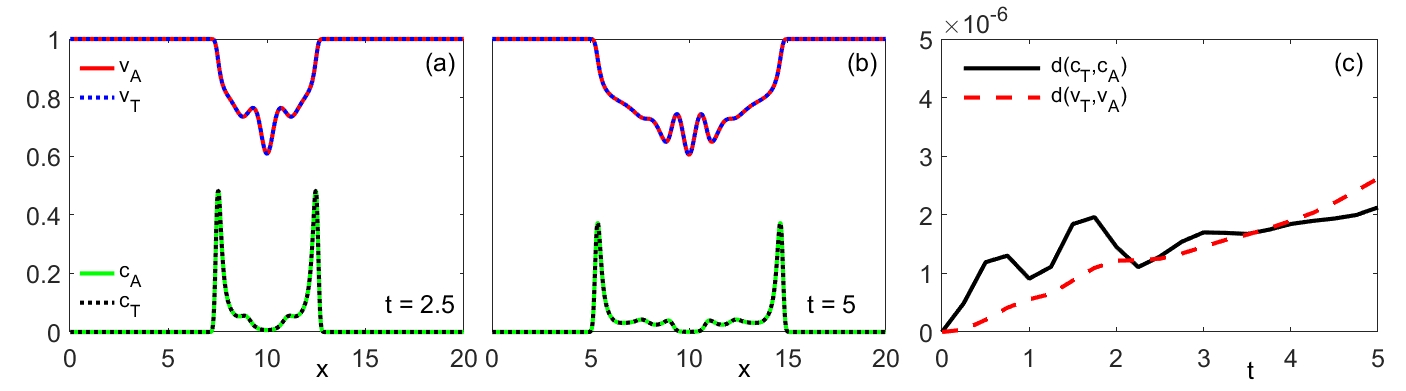
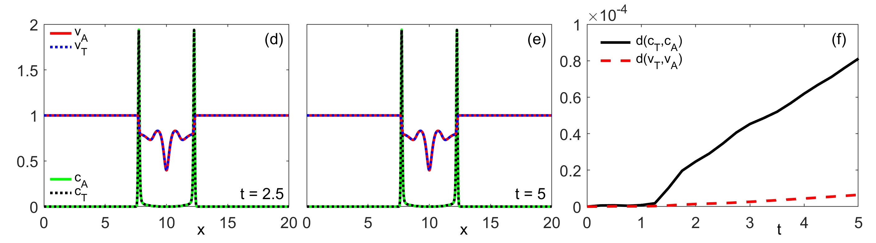
   Figure 1: Comparison between nonlocal formulations 1.1 and 5.1. (a-b) Cell and matrix densities for the models 1.1 and 5.1 at $t=2.5$ and $t=5$. (c) Difference between the solutions. For these simulations we take $\alpha=10$, $r=1$, $D_{c}=0.01$, $\chi=1$, $F_{r}=2$, $f_{c}=0$ and $f_{v}(c,v)=-cv$, along with (a-c) $g(c,v)=10v$, (d-f) $g(c,v)=2.5c+10v$.

   Figure 1 shows the computed solutions under (a-c) negligible cell-cell adhesion ($S_{cc}=0$) and (d-f) moderate cell-cell adhesion ($S_{cc}=S_{cv}/4$). The equivalence of the two formulations is revealed through the negligible difference between solutions, with the distance magnitude attributable to the subtly distinct numerical implementation. Both simulations describe an invasion/infiltration process, in which matrix degradation by the cells generates an adhesive gradient that pulls cells into the acellular surroundings. The impact of cell-cell adhesion is manifested in the compaction of cells at the leading edge into a tight aggregate.

   However, as pointed out in Section 3, differences in the nonlocal formulations can emerge in the vicinity of boundaries. To highlight this we consider an equivalent formulation to Figure 1 (a-c), but with the cells initially placed at the left boundary ($x_{c}=0$ in (6.2)), e.g. suggesting a tumor mass which is concentrated there and whose cells are expected to detach and migrate into the considered 1D domain, travelling from left to right. As stated earlier we impose zero-flux boundary conditions at $x=0$ (and $x=L$), and further suppose $c=v=0$ and $\nabla c=\nabla v$ in the extradomain region ($\mathbb{R}\backslash\Omega$). Representative simulations are shown in Figure 2. They are in agreement with our observation in Example 3.3. Indeed, for this scenario, in the prototypical nonlocal model 1.1-1.2 there is a very large adhesion velocity modulus at $x=0$; the cells are crowded within the tumor mass and their mutual interactions are maintained during the invasion process in a sufficiently strong manner to ensure a collective shift of the still concentrated cell aggregate, with a correspondingly strong tissue degradation in its wake. In the reformulation 5.1-3.2, rather, the adhesion magnitude at $x=0$ is for the same initial condition much lower - suggesting a tumor whose cells are readier to detach and migrate individually. This results in a more diffusive spread, with accordingly less degradation of tissue, and with cell mass remaining available at the original site over a larger time span. The latter scenario is different from the former one, but it seems nevertheless reasonable, as a tumor mass would very often not move as a whole from its original location to another in a relatively short time; moreover, the active cells in a sufficiently large tumor (releasing substantial amounts of acidity) are known to preferentially adopt a migratory phenotype and perform EMT (epithelial-mesenchymal transition), see e.g., [27, 41, 44], which supports the idea of cells moving in a loose way rather than in compact, highly aggregated assemblies . As such, our simulations suggest that, within this particular function- and parameter setting, choosing the adhesion operator in the form 1.2 instead of 3.2 might possibly overestimate the tumor invasion speed and associated healthy tissue degradation, thereby predicting a spatially concentrated tumor and neglecting regions with lower cell densities which can nevertheless trigger tumor recurrence if untreated.

   

   

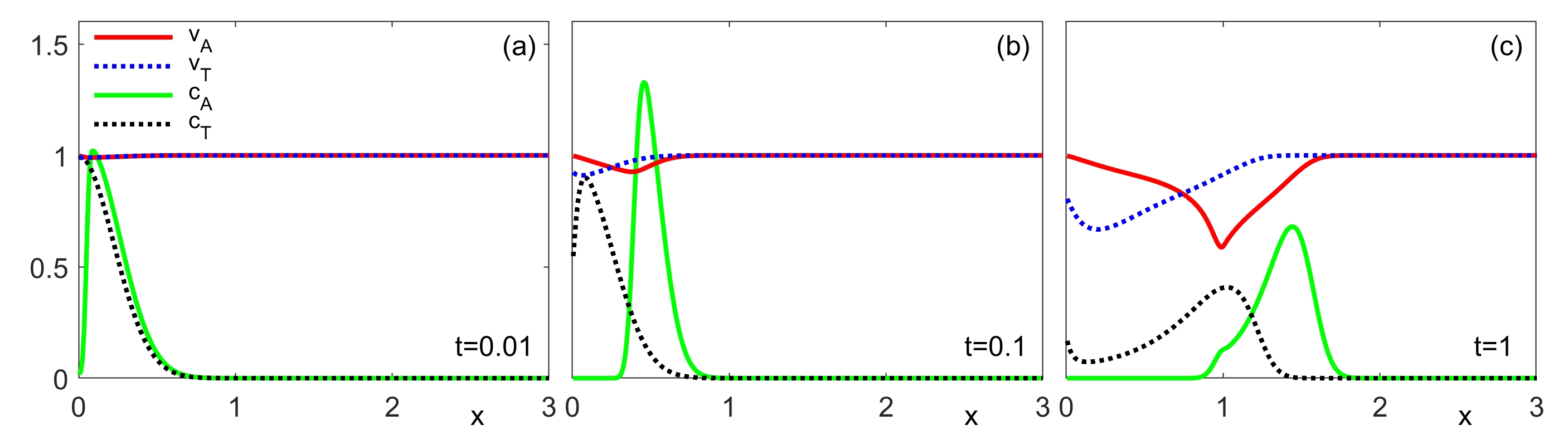
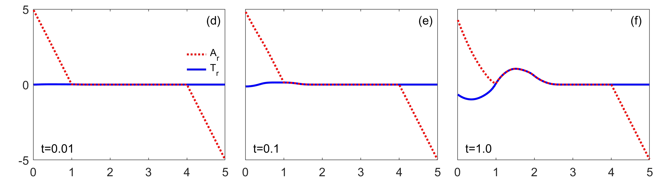
   Figure 2: (a-c) Comparison between nonlocal formulations 1.1 and 5.1 near boundaries. Model as in Figure 1 (a-c), but with the cells initially concentrated at the boundary. (d-f) Comparison of the two forms of nonlocal operator corresponding to the simulations represented in (a-c). The operators are practically identical sufficiently far from the boundary, but can diverge significantly for distances $<r$ from the boundaries.

   6.2 Comparison between nonlocal and local formulation

   Having compared together the original, 1.1, and the new, 5.1, nonlocal formulations, we next consider the extent to which their dynamics can be captured by the classical local formulation 5.2. Note that for nonlocal model simulations we will restrict to the original formulation 1.1, so that we can avail ourselves of an already well-established efficient (in terms of computational time) numerical scheme [23]. Here we use $c_{L}$ and $v_{L}$ to denote solutions to the local formulation and $c_{Ar}$ and $v_{Ar}$ to denote solutions to the nonlocal model with sensing radius $r$. We remark that a large number of related local and nonlocal models have been numerically studied to describe the invasion-type process considered here (e.g. [42, 1, 24, 40]): here the specific focus is to explore the convergence of nonlocal to local form as $r\rightarrow 0$, which, as far as we are aware, has not been systematically investigated.

   As in the first test we use the initial values 6.1 and 6.2, choosing $x_{c}=L/2$, $\alpha=10$ in the latter, and consider the coefficients and functions as proposed in Example 5.5. Under these choices the resultant nonlinear diffusion coefficient for the $c$-equation in the classical local formulation (compare 5.2a) becomes

   $$\tilde{D}_{c}(c,v)=\frac{a^{2}(1+c)^{2}(1+c+v)^{2}-bc(1+cv)(S_{cc}+(S_{cc}-S_{cv})v)}{(1+cv)^{2}(1+c+v)^{2}}.$$ (6.3)

   Notably, this potentially becomes negative under an injudicious combination of adhesive strengths $S_{cc}$, $S_{cv}$, and of $a,b$. Likewise, the actual haptotaxis sensitivity function takes the form

   $$\tilde{\chi}(c,v)=b\frac{S_{cv}+(S_{cv}-S_{cc})c}{(1+cv)(1+c+v)^{2}}.$$ (6.4)

   Again, depending on the relationship between $S_{cc}$ and $S_{cv}$, this can become negative, which would lead to repellent haptotaxis: cells effectively moving away from regions with large ECM gradients, a rather unexpected behaviour. This suggests that cell-tissue adhesions should dominate over cell-cell adhesions, as ’usual’ haptotaxis, i.e. towards the increasing tissue gradient, is known to be an essential component of cell migration, this applying to several types of cells moving through the ECM (tumor cells, mesenchymal stem cells, fibroblasts, endothelial cells, etc.) see e.g. [34, 43, 51] and references therein.

   

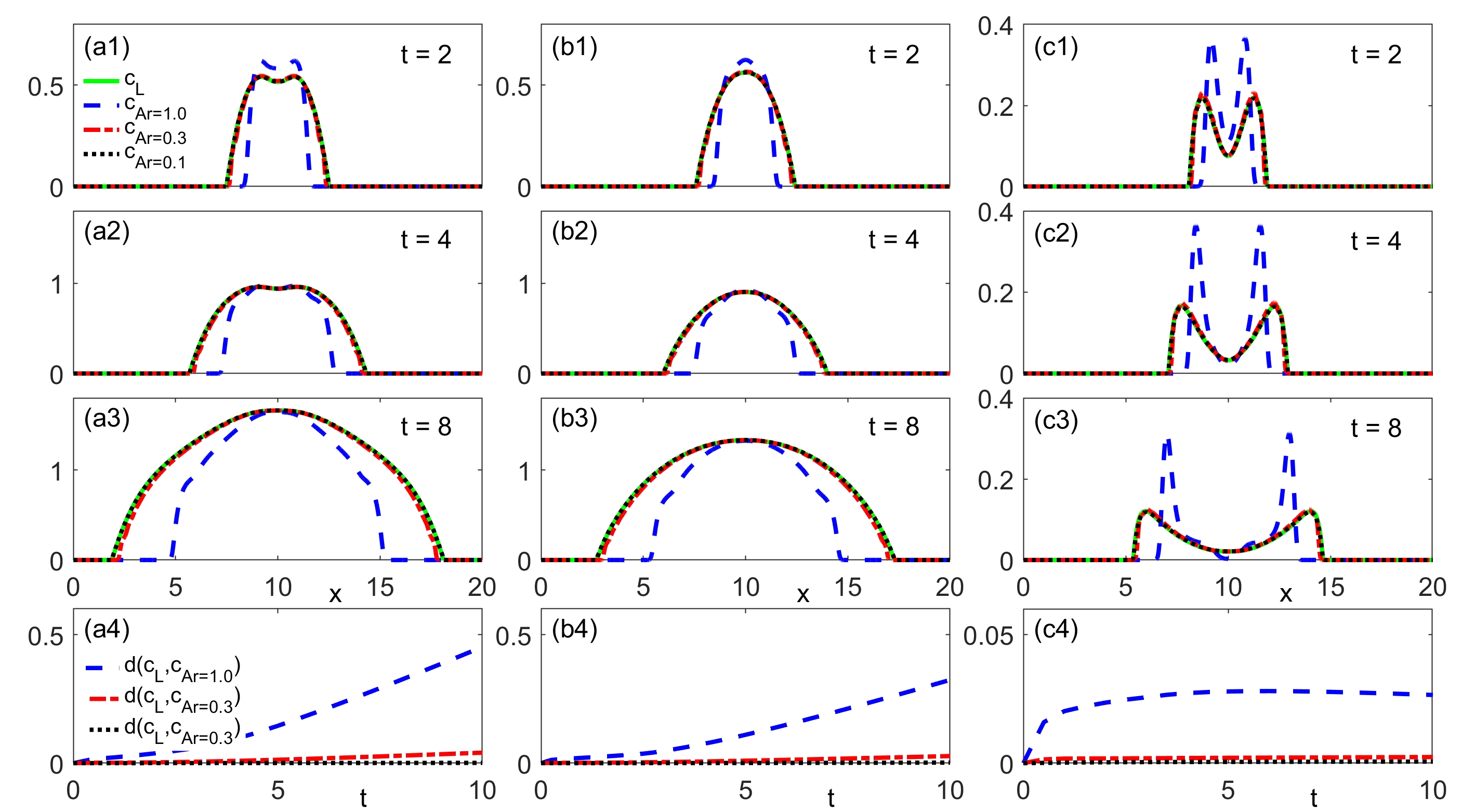
   Figure 3: Convergence between nonlocal and local/classical formulations under negligible cell-cell adhesion, $S_{cc}=0$, $S_{cv}=10$. Functional forms as proposed in Example 5.5, with modifications specified in the subfigures. (a) Solutions for $r=0.1,0.3,1.0$ at (a1) $t=2$, (a2) $t=4$ and (a3) $t=8$; (a4) Distance between local/nonlocal solutions as a function of time. For these simulations, we take $a=0.01$, $b=1$, $\mu_{c}=0.01$, $K_{c}=2$, $\eta_{c}=1$, $\mu_{v}=0$, $\lambda_{v}=1$. (b) Solutions for $r=0.1,0.3,1.0$ at (b1) $t=2$, (b2) $t=4$ and (b3) $t=8$; (b4) Distance between local/nonlocal solutions as a function of time. Parameters as in (a) except $\mu_{v}=1$, $K_{v}=1$. (c) Solutions for $f_{c}=0$ and $f_{v}(c,v)=-cv$, with the other parameters as in (a).

   

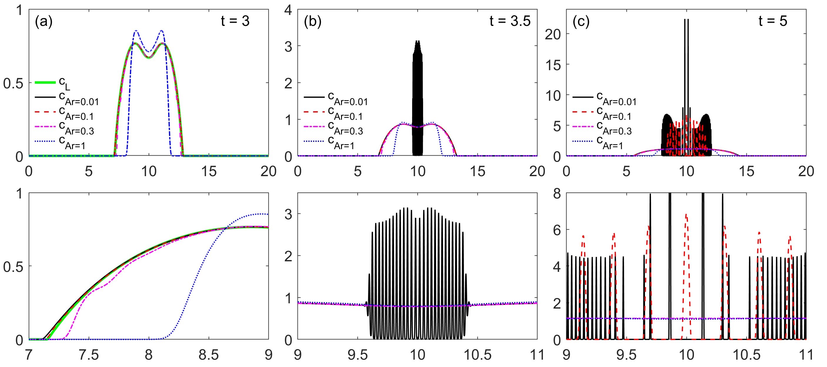
   Figure 4: Time restricted convergence under moderate cell-cell adhesion, $S_{cc}=2.5$, $S_{cv}=10$. Top row shows solutions across the full spatial region ($[0,20]$), the bottom row magnifies a relevant portion for clarity. Solutions to local and nonlocal models under the functional forms proposed in Example 5.5 for $r=0.01,0.1,0.3,1.0$ at (a) $t=3$, (b) $t=3.5$ and (c) $t=5$. In (a) solutions to the local model continue to exist and we observe convergence between local and nonlocal formulations. In (b-c) the solutions to the local model are noncomputable. Nonlocal models, however, can destabilise into a pattern of aggregates. Parameters: $a=0.01$, $b=1$, $\mu_{c}=0.01$, $K_{c}=2$, $\eta_{c}=1$, $\mu_{v}=0$, $\lambda_{v}=1$ and adhesion parameters as above.

   Simulations are plotted in Figure 3 where we show cell densities for the local model ($c_{L}$) and nonlocal model under three sensing radii ($c_{Ar=0.1},c_{Ar=0.3},c_{Ar=1.0}$). In this first set of simulations we assume negligible cell-cell adhesion ($S_{cc}=0$), which automatically ensures positivity for the diffusion coefficient of the equivalent local model, $\tilde{D}_{c}(c,v)$. We note that matrix renewal is absent ($\mu_{v}=0$) in the left-hand column and present ($\mu_{v}>0$) in the central column. In the right-hand column we show the greater generality of the results under vastly simplified kinetics, specifically setting $f_{c}(c,v)=0$ and $f_{v}(c,v)=-cv$ (with the other functional forms as in Example 5.5). Simulations highlight the convergence between local and nonlocal models as $r\rightarrow 0$: for $r=0.1$, the solution differences become negligible. However, distinctions emerge for large $r$, where we can expect significant discrepancy between the solutions. This suggests that the local model fails to accurately predict the behaviour in cases where cells sample over relatively large regions of their local environment.

   Next, we extend to include a degree of cell-cell adhesion, setting functions and parameters as in Figure 3, except now $S_{cc}>0$. Notably this raises the possibility of a negative diffusion coefficient in the classical formulation and subsequent illposedness. Solutions under a representative set of parameters are shown in Figure 4. For $t$ below some critical time we observe convergence as before, with the nonlocal formulation converging to solutions of the local model as $r\rightarrow 0$. However, continued matrix degradation further depletes $v$, with the result that (6.3) can become negative. At this point (in this case $t\approx 3.2\ldots$) the local model becomes illposed and its solutions become incomputable (implying nonexistence of solutions). However, the nonlocal formulation appears to preserve wellposedness, consistent with previous theoretical studies where extending to a nonlocal formulation regularises a singular local model (e.g. [29]). Solutions to the nonlocal model instead destabilise into a quasi-periodic pattern of cell aggregations, maintained through the cell-cell adhesion, and with a wavelength shrinking as $r\rightarrow 0$.

   Finally, we remark that convergence of solutions extends beyond the specific functional forms and, as a representative example, we consider a minimalist setting based on linear/constant forms. Specifically, we set $D_{c}=a$ (constant), $\chi=1$, $f_{c}=0$, $g(c,v)=S_{cc}c+S_{cv}v$ and $f_{v}(c,v)=-\mu cv$. In this scenario, the diffusion and haptotaxis coefficients for the classical local formulation 5.2 reduce to

   $$\tilde{D}_{c}(c,v)=a-S_{cc}c\quad\mbox{and}\quad\tilde{\chi}(c,v)=S_{cv}.$$ (6.5)

   Positivity is only guaranteed under appropriate parameter selection. Such a case is illustrated in Figure 5 (a) where we assume negligible cell-cell adhesion ($S_{cc}=0$). Clearly, we observe convergence between the nonlocal and local formulations as $r\rightarrow 0$. Inappropriate parameter selection, however, generates backward diffusion in the local model and solutions are consequently incomputable. Under such scenarios, however, solutions to the nonlocal model appear to exist: Figure 5 (b) plots the behaviour under shrinking $r$. In all cases considered in this test the cells do not reach the boundary region where the difference between the nonlocal formulations 1.1 and 5.1 can play a role. Thus, we expect the same solution if reformulation 5.1 is applied instead.

   

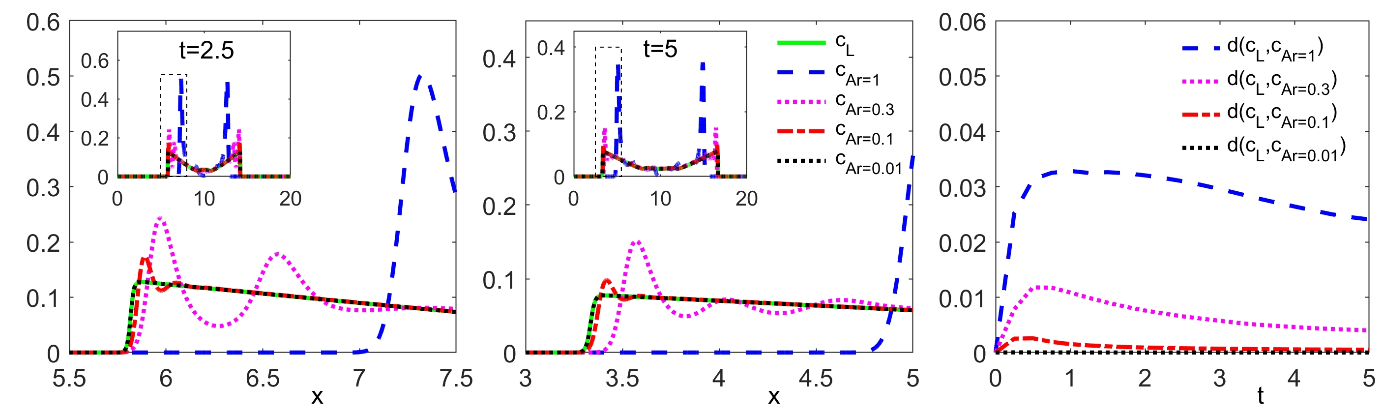
   Figure 5: Convergence between nonlocal and local/classical formulations under a set of minimalistic linear functional forms ($D_{c}=0.01,\chi=1,f_{c}=0,g(c,v)=S_{cc}c+S_{cv}v,f_{v}(c,v)=-\mu cv$). (a) Negligible cell-cell adhesion, $S_{cc}=0,S_{cv}=10$: solutions shown at (left) $t=2.5$ and (middle) $t=5$, with the distance between solutions to the nonlocal and local model shown in the right panel.

   7 Discussion

   In this work we provide a rigorous limit procedure which links nonlocal models involving adhesion or a nonlocal form of chemotaxis gradient to their local counterparts featuring haptotaxis, respectively chemotaxis in the usual sense. As such, our paper closes a gap in the existing literature. Moreover, it offers a unified treatment of the two types of models and extends the previous mathematical framework to settings allowing for more general, solution dependent, coefficient functions (diffusion, tactic sensitivity, adhesion velocity, nonlocal taxis gradient, etc.). Finally, we provide simulations illustrating some of our theoretical findings in 1D.

   Our reformulations in terms of $\mathcal{T}_{r}$ and $\mathcal{S}_{r}$ reveal the tight relationship between the nonlocal operators $\mathcal{A}_{r}$ and $\mathring{\nabla}_{r}$ and the (local) gradient. This suggests that both nonlocal descriptions (adhesion, chemotaxis) actually encompass the dependence on the signal gradients rather than on the signal concentration/density itself, which is in line with the biological phenomenon. Indeed, through their transmembrane elements (e.g. receptors, ion channels etc.) the cells are mainly able to perceive and respond to differences in the signal at various locations or within more or less confined areas rather than measure effective signal concentrations. Along with the mentioned solution dependency of the nonlocal model coefficients, the influence of the gradient possibly reflects into contributions of the adhesion/nonlocal chemotaxis to the (nonlinear) diffusion in the local setting obtained through the limiting procedure.

   The set $\Omega_{r}$ (as introduced in Section 2) can be regarded as the ’domain of restricted sensing’, meaning that there cells a priori sense only what happens inside $\Omega$, the domain of interest. The measure of this subdomain is a decreasing function of the sensing radius $r$. When $r\to 0$ the set $\Omega_{r}$ tends to cover the whole domain $\Omega$, whereas as $r$ increases the cells can sense at increasingly larger distances; correspondingly, $\Omega_{r}$ shrinks. For $r>\operatorname{diam}(\Omega)$ the restricted sensing domain is empty: everywhere in $\Omega$ the cells can perceive signals not only from any point within $\Omega$ but potentially also from the outside. In this paper, however, we look at models with no-flux boundary conditions. This corresponds, e.g., to the impenetrability of the walls of a Petri dish or that of comparatively hard barriers limiting the areas populated by migrating cells, e.g. bones or cartilage material. As a result, the cells in the boundary layer $\Omega\setminus\Omega_{r}$ have a much reduced ability to stretch their protrusions outside $\Omega$ and thus gain little information from without. To simplify matters, we assume in this work that there is no such information or it is insufficient to trigger any change in their behaviour. In the definitions of $\mathcal{T}_{r}$ and $\mathcal{S}_{r}$ this corresponds to the integrands being set to zero in $\Omega\backslash\overline{\Omega}_{r}$.

   It is important to note that for points $x\in\Omega\backslash\overline{\Omega}_{r}$ the influence of a signal $p$ in a direction $y\in S_{1}$ is not taken into account by $\mathring{\nabla}_{r}$ at all if $x+ry\not\in\overline{\Omega}$. If $\mathcal{S}_{r}$ is used instead, then its contribution to the average is given by

   $$\tilde{y}:=n\left(\int_{0}^{1}\chi_{\Omega}\nabla p(x+rsy)\,ds\cdot y\right)y.$$

   Thus, thanks to integration w.r.t. $s$, the resulting vector $\tilde{y}$ assembles the impact of those parts of the segment connecting $x$ and $x+ry$ which are contained in $\Omega$. It is parallel to $y$, and it may have the same or the opposite orientation. In particular this means that although for a certain range of directions large parts of the sensing region of a cell are actually outside $\Omega$, this may still strongly influence the speed and actual direction of the drift. The effect of integration w.r.t. $s$ in $\mathcal{T}_{r}$ is less obvious, since in this case the average w.r.t. $y$ is computed over the ball $B_{1}$. This already achieves the covering of the whole sensing region by allowing a cell to gather information about the signal not only in any direction $y/{|y|}$, but also at any distance less than $r$. The additional integration over the path $x+rsy$, $s\in[0,1]$, appears to mean that cells at $x\in\Omega_{r}$ are able to measure the average of the signal gradient all along such line segment rather than its value directly at the ending point. Indeed, from a biological viewpoint this description seems to make more sense, as cells do not jump from one position to another, nor do they send out their protrusions in a discontinuous way bypassing certain space points along a chosen direction. Averages over cell paths are then averaged w.r.t. $y$, which finally determines the direction of population movement. Example 3.4 indicates that the effect of even an extremely concentrated signal gradient is mollified by averaging. This agrees with our expectations from using non-locality. In higher dimensions $n\geq 2$, the two-stage averaging in ${\cal T}_{r}$ (w.r.t. $s$ and $y$) produces a direction field which is smooth away from the concentration point and also weakens but still keeps the singularity there. In contrast, averaging only w.r.t. $y$ leads instead to jump discontinuities at a unit distance from the accumulation point. Moreover, we remark that without integrating w.r.t. $s$ in ${\cal T}_{r}(\nabla\cdot)$ one cannot regain ${\cal A}_{r}$.

   The effect observed in Example 3.3 further supports the conjecture that the nonlocal operators which act directly on the signal gradients might actually be a more appropriate modelling tool. While inside the subdomain $\Omega_{r}$ there is no difference (recall Lemmas 3.1 and 3.2), inside the boundary layer $\Omega\backslash\overline{\Omega}_{r}$ the limiting behaviour as $r\rightarrow 0$ is qualitatively distinct. Indeed, Example 3.3 shows that using, e.g., $\mathcal{A}_{r}$, leads, for $r\rightarrow 0$, to unnatural sharp singularities at the boundary of $\Omega$ even in the absence of signal gradients, whereas this does not happen if $\mathcal{T}_{r}$ is used instead. Simulations in Subsection 6.1 (see Figure 2) confirm our theoretical findings and show a substantial difference between the solutions obtained with the two nonlocal formulations involving 1.2 and 3.2, respectively. The choice 3.2 is motivated above all from a mathematical viewpoint (as it enables a rigorous, well-justified passage to the limit for $r\to 0$), but it also seems to make sense biologically, as our above comments and the simulations performed for the particular setting in Subsection 6.1 suggest.

   Acknowledgement

   MK and CS acknowledge the partial support of the research initiative Mathematics Applied to Real World Challenges (MathApp) of the TU Kaiserslautern. CS also acknowledges funding by the Federal Ministry of Education and Research (BMBF) in the project GlioMaTh.

References

• [1] A. R. A. Anderson, M. A. J. Chaplain, E. L. Newman, R. J. C. Steele, and M. Thompson, A. Mathematical modelling of tumour invasion and metastasis. Computational and mathematical methods in medicine, 2(2):129–154, 2000.
• [2] N. J. Armstrong, K. J. Painter, and J. A. Sherratt. A continuum approach to modelling cell-cell adhesion. J. Theoret. Biol., 243(1):98–113, 2006.
• [3] G. Bell. Models for the specific adhesion of cells to cells. Science, 200(4342):618–627, 1978.
• [4] G. Bell, M. Dembo, and P. Bongrand. Cell adhesion. competition between nonspecific repulsion and specific bonding. Biophysical Journal, 45(6):1051 – 1064, 1984.
• [5] N. Bellomo, A. Bellouquid, Y. Tao, and M. Winkler. Toward a mathematical theory of keller-segel models of pattern formation in biological tissues. Math. Models Meth. Appl. Sci., 25(9):1663–1763, 2015.
• [6] V. Bitsouni, D. Trucu, M. A. J. Chaplain, and R. Eftimie. Aggregation and travelling wave dynamics in a two-population model of cancer cell growth and invasion. Mathematical Medicine and Biology: A Journal of the IMA, 35(4):541–577, 01 2018.
• [7] A. Buttenschön and T. Hillen. Nonlocal adhesion models for microorganisms on bounded domains, preprint.
• [8] A. Buttenschön, T. Hillen, A. Gerisch, and K. J. Painter. A space-jump derivation for non-local models of cell-cell adhesion and non-local chemotaxis. J. Math. Biol., 76(1-2):429–456, 2018.
• [9] J. Carrillo, H. Murakawa, M. Sato, H. Togashi, and O. Trush. A population dynamics model of cell-cell adhesion incorporating population pressure and density saturation. J. Theor. Biol., 474:14–24, 2019.
• [10] M. Chaplain, M. Lachowicz, Z. Szymanska, and D. Wrzosek. Mathematical modelling of cancer invasion: The importance of cell-cell adhesion and cell-matrix adhesion. Mathematical Models and Methods in Applied Sciences, 21(04):719–743, 2011.
• [11] L. Chen, K. Painter, C. Surulescu, and A. Zhigun. Mathematical models for cell migration: a nonlocal perspective, 2019.
• [12] R. B. Dickinson and R. T. Tranquillo. A stochastic model for adhesion-mediated cell random motility and haptotaxis. Journal of Mathematical Biology, 31(6):563–600, 1993.
• [13] P. DiMilla, K. Barbee, and D. Lauffenburger. Mathematical model for the effects of adhesion and mechanics on cell migration speed. Biophysical Journal, 60(1):15 – 37, 1991.
• [14] P. Domschke, D. Trucu, A. Gerisch, and M. A. J. Chaplain. Mathematical modelling of cancer invasion: implications of cell adhesion variability for tumour infiltrative growth patterns. J. Theoret. Biol., 361:41–60, 2014.
• [15] P. Domschke, D. Trucu, A. Gerisch, and M. A. J. Chaplain. Structured models of cell migration incorporating molecular binding processes. J. Math. Biol., 75(6-7):1517–1561, 2017.
• [16] J. Dyson, S. Gourley, and G. Webb. A non-local evolution equation model of cell-cell adhesion in higher dimensional space. Journal of biological dynamics, 7:68–87, 2013.
• [17] J. Dyson, S. A. Gourley, R. Villella-Bressan, and G. F. Webb. Existence and asymptotic properties of solutions of a nonlocal evolution equation modeling cell-cell adhesion. SIAM J. Math. Anal., 42(4):1784–1804, 2010.
• [18] R. Eftimie. Hyperbolic and Kinetic Models for Self-organised Biological Aggregations. A Modelling and Pattern Formation Approach. Springer, Cham, 2018.
• [19] C. Engwer, C. Stinner, and C. Surulescu. On a structured multiscale model for acid-mediated tumor invasion: the effects of adhesion and proliferation. Math. Models Methods Appl. Sci., 27(7):1355–1390, 2017.
• [20] D. S. Eom and D. M. Parichy. A macrophage relay for long-distance signaling during postembryonic tissue remodeling. Science, 355(6331):1317–1320, 2017.
• [21] L. C. Evans. Weak convergence methods for nonlinear partial differential equations, volume 74 of CBMS Regional Conference Series in Mathematics. Published for the Conference Board of the Mathematical Sciences, Washington, DC; by the American Mathematical Society, Providence, RI, 1990.
• [22] G. Garcia and C. Parent. Signal relay during chemotaxis. Journal of Microscopy, 231(3):529–534, 2008.
• [23] A. Gerisch. On the approximation and efficient evaluation of integral terms in PDE models of cell adhesion. IMA Journal of Numerical Analysis, 30(1):173–194, 01 2010.
• [24] A. Gerisch and M. A. J. Chaplain. Mathematical modelling of cancer cell invasion of tissue: local and non-local models and the effect of adhesion. J. Theoret. Biol., 250(4):684–704, 2008.
• [25] A. Gerisch and K. J. Painter. Mathematical modeling of cell adhesion and its applications to developmental biology and cancer invasion. 2010.
• [26] L. González-Méndez, I. Seijo-Barandiarán, and I. Guerrero. Cytoneme-mediated cell-cell contacts for hedgehog reception. eLife, 6:e24045, 2017.
• [27] S. C. Gupta and Y.-Y. Mo. Abstract 168: Malat1 is crucial for epithelial-mesenchymal transition of breast cancer cells in acidic microenvironment. Cancer Research, 75(15 Supplement):168–168, 2015.
• [28] T. Hillen. A classification of spikes and plateaus. SIAM Rev., 49(1):35–51, 2007.
• [29] T. Hillen, K. Painter, and C. Schmeiser. Global existence for chemotaxis with finite sampling radius. Discrete Contin. Dyn. Syst. Ser. B, 7(1):125–144.
• [30] T. Hillen, K. Painter, and M. Winkler. Global solvability and explicit bounds for non-local adhesion models. European Journal of Applied Mathematics, 29(04):1–40, 2018.
• [31] N. I. Kavallaris and T. Suzuki. Non-local partial differential equations for engineering and biology, volume 31 of Mathematics for Industry (Tokyo). Springer, Cham, 2018. Mathematical modeling and analysis.
• [32] E. Kuusela and W. Alt. Continuum model of cell adhesion and migration. Journal of Mathematical Biology, 58(1):135, 2008.
• [33] O. Ladyzhenskaya, V. Solonnikov, and N. Ural’tseva. Linear and quasi-linear equations of parabolic type. Translated from the Russian by S. Smith. Translations of Mathematical Monographs. 23. Providence, RI: American Mathematical Society (AMS). XI, 648 p. (1968)., 1968.
• [34] L. Lamalice, F. Le Boeuf, and J. Huot. Endothelial cell migration during angiogenesis. Circulation Research, 100:782 – 794, 2007.
• [35] J.-L. Lions. Quelques méthodes de résolution des problèmes aux limites non linéaires. Dunod, Gauthier-Villars, Paris, 1969.
• [36] N. Loy and L. Preziosi. Kinetic models with non-local sensing determining cell polarization and speed according to independent cues. arXiv:1906.11039, 2019.
• [37] P. Lu, V. Weaver, and Z. Werb. The extracellular matrix: A dynamic niche in cancer progression. J. Cell Biol., 196:395–406, 2012.
• [38] H. Murakawa and H. Togashi. Continuous models for cell-cell adhesion. Journal of Theoretical Biology, 374:1–12, 2015.
• [39] H. Othmer and T. Hillen. The diffusion limit of transport equations ii: chemotaxis equations. SIAM J. Appl. Math., 62:1122–1250, 2002.
• [40] K. J. Painter, N. J. Armstrong, and J. A. Sherratt. The impact of adhesion on cellular invasion processes in cancer and development. Journal of Theoretical Biology, 264(3):1057 – 1067, 2010.
• [41] S. Peppicelli, F. Bianchini, E. Torre, and L. Calorini. Contribution of acidic melanoma cells undergoing epithelial-to-mesenchymal transition to aggressiveness of non-acidic melanoma cells. Clinical & Experimental Metastasis, 31(4):423–433, Jan. 2014.
• [42] A. J. Perumpanani, J. A. Sherratt, J. Norbury, and H. M. Byrne. Biological inferences from a mathematical model for malignant invasion. Invasion Metastasis, 16(4-5):209–221, 1996.
• [43] M. Pickup, J. Mouw, and V. Weaver. The extracellular matrix modulates the hallmarks of cancer. EMBO reports, 15:1243–1253, 2014.
• [44] E. Prieto-García, C. V. Díaz-García, I. García-Ruiz, and M. T. Agulló-Ortuño. Epithelial-to-mesenchymal transition in tumor progression. Medical Oncology, 34(7), May 2017.
• [45] I. Sáenz-de Santa-María, C. Bernardo-Castiñeira, E. Enciso, I. García-Moreno, J. Chiara, C. Suarez, and M.-D. Chiara. Control of long-distance cell-to-cell communication and autophagosome transfer in squamous cell carcinoma via tunneling nanotubes. Oncotarget, 8:20939–20960, 2017.
• [46] J. Sherratt, S. Gourley, N. Armstrong, and K. Painter. Boundedness of solutions of a non-local reaction-diffusion model for adhesion in cell aggregation and cancer invasion. European Journal of Applied Mathematics, 20(1):123–144, 2009.
• [47] R. E. Showalter. Monotone Operators in Banach Space and Nonlinear Partial Differential Equations, volume 49 of Mathematical Surveys and Monographs. American Mathematical Society, 1997.
• [48] R. Temam. Navier-Stokes equations: theory and numerical analysis, volume 343. American Mathematical Soc., 2001.
• [49] A. Uatay. Multiscale Mathematical Modeling of Cell Migration: From Single Cells to Populations. PhD thesis, TU Kaiserslautern, 2019.
• [50] M. Ward and D. Hammer. A theoretical analysis for the effect of focal contact formation on cell-substrate attachment strength. Biophysical Journal, 64(3):936 – 959, 1993.
• [51] J. H. Wen, O. Choi, H. Taylor-Weiner, A. Fuhrmann, J. V. Karpiak, A. Almutairi, and A. J. Engler. Haptotaxis is cell type specific and limited by substrate adhesiveness. Cell Mol. Bioeng., 8(4):530 – 542, 2015.
• [52] E. Zeidler. Nonlinear functional analysis and its applications. I. Springer-Verlag, New York, 1986. Fixed-point theorems, Translated from the German by Peter R. Wadsack.