A Parallel Augmented Subspace Method for Eigenvalue Problems

Abstract

A type of parallel augmented subspace scheme for eigenvalue problems is proposed by using coarse space in the multigrid method. With the help of coarse space in multigrid method, solving the eigenvalue problem in the finest space is decomposed into solving the standard linear boundary value problems and very low dimensional eigenvalue problems. The computational efficiency can be improved since there is no direct eigenvalue solving in the finest space and the multigrid method can act as the solver for the deduced linear boundary value problems. Furthermore, for different eigenvalues, the corresponding boundary value problem and low dimensional eigenvalue problem can be solved in the parallel way since they are independent of each other and there exists no data exchanging. This property means that we do not need to do the orthogonalization in the highest dimensional spaces. This is the main aim of this paper since avoiding orthogonalization can improve the scalability of the proposed numerical method. Some numerical examples are provided to validate the proposed parallel augmented subspace method.

Keywords. eigenvalue problems, parallel augmented subspace method, multigrid method, parallel computing.

AMS subject classifications. 65N30, 65N25, 65L15, 65B99.

1 Introduction

Solving large scale eigenvalue problems is one of fundamental problems in modern science and engineering society. It is always a very difficult task to solve high-dimensional eigenvalue problems which come from practical physical and chemical sciences. Compared with boundary value problems, there are less efficient numerical methods for solving eigenvalue problems with optimal complexity. The large scale eigenvalue problems pose significant challenges for scientific computing. In order to solve these large scale sparse eigenvalue problems, Krylov subspace type methods (Implicitly Restarted Lanczos/Arnoldi Method (IRLM/IRAM) [29]), the Preconditioned INVerse ITeration (PINVIT) method [14, 8, 20], the Locally Optimal Block Preconditioned Conjugate Gradient (LOBPCG) method [21, 23], and the Jacobi-Davidson-type techniques [4] have been developed. All these popular methods include the orthogonalization step which is a bottleneck for designing efficient parallel schemes for determining relatively many eigenpairs. Recently, a type of multilevel correction method is proposed for solving eigenvalue problems in [24, 32, 33]. In this multilevel correction scheme, there exists an augmented subspace which is constructed with the help of coarse space from the multigrid method. The application of this augmented subspace leads to that the solution of eigenvalue problem on the final level of mesh can be reduced to a series of solutions of boundary value problems on the multilevel meshes and a series of solutions of the eigenvalue problem on the low dimensional augmented subspace. The multilevel correction method gives a way to construct the multigrid method for eigenvalue problems.

It is well known that the multigrid method [10, 28, 35] provides an optimal numerical method for linear elliptic boundary value problems. The error bounds of the approximate solution obtained from these efficient numerical algorithms are comparable to the theoretical bounds determined by the finite element discretization, while the amount of computational work involved is only proportional to the number of unknowns in the discretized equations. For more details of the multigrid method, please refer to [5, 6, 7, 9, 10, 16, 17, 25, 27, 28, 35, 36] and the references cited therein.

This paper aims to design a type of parallel method for eigenvalue problems with the help of the coarse space from the multigrid method. It is well known that there exist many work considering the applications of multigrid method for eigenvalue problems. For example, there have existed applications of the multigrid method to the PINVIT and LOBPCG methods. But, in these applications, the multigrid method only acts as the precondition for the included linear equations. This means that the multigrid method only improves the efficiency of the inner iteration and does not change the outer iteration. Unfortunately, in these state-of-the-art, the applications of multigrid method do not deduce a new eigensolver. The idea of designing the parallel augmented subspace method for eigenvalue problems is based on the combination of the multilevel correction method [24, 32, 33, 34] and parallel computing technique. With the help of coarse space in multigrid method, the eigenvalue problem solving is transformed into a series of solutions of the corresponding linear boundary value problems on the sequence of finite element spaces and eigenvalue problems on a very low dimensional augmented space. Further, in order to improve the parallel scalability, the approximate eigenpairs are computed independently by a correction process. This property means there is no orthogonalization in the highest dimensional space which account for a large portion of wall time in the parallel computation.

An outline of the paper goes as follows. In Section 2, we introduce the finite element method for the eigenvalue problem and the corresponding basic error estimates. A type of parallel augmented subspace method for solving the eigenvalue problem by finite element method is given in Section 3, and the corresponding computational work estimate are given in Section 4. In Section 5, four numerical examples are presented to validate our theoretical analysis. Some concluding remarks are given in the last section.

2 Finite element method for eigenvalue problem

This section is devoted to introducing some notation and the standard finite element method for the eigenvalue problem. In this paper, we shall use the standard notation for Sobolev spaces $W^{s,p}(\Omega)$ and their associated norms and semi-norms (cf. [1]). For $p=2$, we denote $H^{s}(\Omega)=W^{s,2}(\Omega)$ and $H_{0}^{1}(\Omega)=\{v\in H^{1}(\Omega):\ v|_{\partial\Omega}=0\}$, where $v|_{\Omega}=0$ is in the sense of trace, $\|\cdot\|_{s,\Omega}=\|\cdot\|_{s,2,\Omega}$. In some places, $\|\cdot\|_{s,2,\Omega}$ should be viewed as piecewise defined if it is necessary. The letter $C$ (with or without subscripts) denotes a generic positive constant which may be different at its different occurrences through the paper.

For simplicity, we consider the following model problem to illustrate the main idea: Find $(\lambda,u)$ such that

$$\left\{\begin{array}[]{rcl}-\nabla\cdot(\mathcal{A}\nabla u)&=&\lambda u,\quad{\rm in}\ \Omega,\\ u&=&0,\ \ \quad{\rm on}\ \partial\Omega,\end{array}\right.$$ (2.1)

where $\mathcal{A}$ is a symmetric and positive definite matrix with suitable regularity, $\Omega\subset\mathcal{R}^{d}\ (d=2,3)$ is a bounded domain with Lipschitz boundary $\partial\Omega$.

In order to use the finite element method to solve the eigenvalue problem (2.1), we need to define the corresponding variational form as follows: Find $(\lambda,u)\in\mathcal{R}\times V$ such that $a(u,u)=1$ and

$$a(u,v)=\lambda b(u,v),\quad\forall v\in V,$$ (2.2)

where $V:=H_{0}^{1}(\Omega)$ and

$$a(u,v)=\int_{\Omega}\mathcal{A}\nabla u\cdot\nabla vd\Omega,\ \ \ \ \ \ b(u,v)=\int_{\Omega}uvd\Omega.$$ (2.3)

The norms $\|\cdot\|_{a}$ and $\|\cdot\|_{b}$ are defined by

$$\|v\|_{a}=\sqrt{a(v,v)}\ \ \ \ \ {\rm and}\ \ \ \ \ \|v\|_{b}=\sqrt{b(v,v)}.$$

It is well known that the eigenvalue problem (2.2) has an eigenvalue sequence $\{\lambda_{j}\}$ (cf. [2, 11]):

$$0<\lambda_{1}\leq\lambda_{2}\leq\cdots\leq\lambda_{k}\leq\cdots,\ \ \ \lim_{k\rightarrow\infty}\lambda_{k}=\infty,$$

and associated eigenfunctions

$$u_{1},u_{2},\cdots,u_{k},\cdots,$$

where $a(u_{i},u_{j})=\delta_{ij}$ ($\delta_{ij}$ denotes the Kronecker function). In the sequence $\{\lambda_{j}\}$, the $\lambda_{j}$ are repeated according to their geometric multiplicity. For our analysis, recall the following definition for the smallest eigenvalue (see [3, 11])

$$\lambda_{1}=\min_{0\neq w\in V}\frac{a(w,w)}{b(w,w)}.$$ (2.4)

Now, let us define the finite element approximations of the problem (2.2). First we generate a shape-regular triangulation $\mathcal{T}_{h}$ of the computing domain $\Omega\subset\mathcal{R}^{d}\ (d=2,3)$ into triangles or rectangles for $d=2$ (tetrahedrons or hexahedrons for $d=3$). The diameter of a cell $K\in\mathcal{T}_{h}$ is denoted by $h_{K}$ and the mesh size $h$ describes the maximal diameter of all cells $K\in\mathcal{T}_{h}$. Based on the mesh $\mathcal{T}_{h}$, we can construct a finite element space denoted by $V_{h}\subset V$. For simplicity, we set $V_{h}$ as the linear finite element space which is defined as follows

$$V_{h}=\big{\{}v_{h}\in C(\Omega)\ \big{|}\ v_{h}|_{K}\in\mathcal{P}_{1},\ \ \forall K\in\mathcal{T}_{h}\big{\}}\cap H^{1}_{0}(\Omega),$$ (2.5)

where $\mathcal{P}_{1}$ denotes the linear function space.

The standard finite element scheme for eigenvalue problem (2.2) is: Find $(\bar{\lambda}_{h},\bar{u}_{h})\in\mathcal{R}\times V_{h}$ such that $a(\bar{u}_{h},\bar{u}_{h})=1$ and

$$a(\bar{u}_{h},v_{h})=\bar{\lambda}_{h}b(\bar{u}_{h},v_{h}),\quad\ \ \ \forall v_{h}\in V_{h}.$$ (2.6)

From [2, 3], the discrete eigenvalue problem (2.6) has eigenvalues:

$$0<\bar{\lambda}_{1,h}\leq\bar{\lambda}_{2,h}\leq\cdots\leq\bar{\lambda}_{k,h}\leq\cdots\leq\bar{\lambda}_{N_{h},h},$$

and corresponding eigenfunctions

$$\bar{u}_{1,h},\bar{u}_{2,h},\cdots,\bar{u}_{k,h},\cdots,\bar{u}_{N_{h},h},$$ (2.7)

where $a(\bar{u}_{i,h},\bar{u}_{j,h})=\delta_{ij}$, $1\leq i,j\leq N_{h}$ ($N_{h}$ is the dimension of the finite element space $V_{h}$). From the min-max principle [2, 3], the eigenvalues of (2.6) provide upper bounds for the first $N_{h}$ eigenvalues of (2.2)

$$\lambda_{i}\leq\bar{\lambda}_{i,h},\ \ \ \ 1\leq i\leq N_{h}.$$ (2.8)

In order to measure the error of the finite element space to the desired function, we define the following notation

$$\delta(w,V_{h})=\inf_{v_{h}\in V_{h}}\|w-v_{h}\|_{a},\ \ \ {\rm for}\ w\in V.$$ (2.9)

In this paper, we also need the following quantity for error analysis:

$$\eta(V_{h}) = \sup_{\begin{subarray}{c}f\in L^{2}(\Omega)\\ \|f\|_{b}=1\end{subarray}}\inf_{v_{h}\in V_{h}}\|Tf-v_{h}\|_{a},$$ (2.10)

where $T:L^{2}(\Omega)\rightarrow V$ is defined as

$${\color[rgb]{0,0,0}a(Tf,v)=b(f,v),\ \ \ \ \ \forall v\in V\ \ {\rm for}\ f\in L^{2}(\Omega).}$$ (2.11)

In order to understand the method more clearly, we state the error estimate for the eigenpair approximation by the finite element method. For this aim, we define the finite element projection $\mathcal{P}_{h}$ as follows

$${\color[rgb]{0,0,0}a(\mathcal{P}_{h}w,v_{h})=a(w,v_{h}),\ \ \ \ \forall v_{h}\in V_{h}\ \ {\rm for}\ w\in V.}$$ (2.12)

It is obvious that

$${\color[rgb]{0,0,0}\|u-\mathcal{P}_{h}u\|_{a}=\inf_{w_{h}\in V_{h}}\|u-w_{h}\|_{a}=\delta(u,V_{h}),\ \ \ \forall u\in V.}$$ (2.13)

The following Rayleigh quotient expansion of the eigenvalue error is the tool to obtain the error estimates of eigenvalue approximations.

Lemma 2.1.

([2]) Assume $(\lambda,u)$ is an eigenpair of the eigenvalue problem (2.2). Then for any $w\in V\backslash\{0\}$, the following expansion holds:

$$\frac{a(w,w)}{b(w,w)}-\lambda=\frac{a(w-u,w-u)}{b(w,w)}-\lambda\frac{b(w-u,w-u)}{b(w,w)}.$$ (2.14)

The following lemma is similar to the corresponding results in [3, 11, 34]. Since this paper considers the parallel scheme for different eigenpair, we state the error estimates for any single eigenpair. In order to analyze and understand the proposed numerical algorithms in this paper, we use the following error estimates from [34] which include only explicit constants. For the proof, please refer to [34].

Lemma 2.2.

([34, Lemma 3.3]) Let $(\lambda,u)$ denote an exact eigenpair of the eigenvalue problem (2.2). Assume the eigenpair approximation $(\bar{\lambda}_{i,h},\bar{u}_{i,h})$ has the property that $\bar{\mu}_{i,h}=1/\bar{\lambda}_{i,h}$ is closest to $\mu=1/\lambda$. The corresponding spectral projectors $E_{i,h}:V\mapsto{\rm span}\{\bar{u}_{i,h}\}$ and $E:V\mapsto{\rm span}\{u\}$ are defined as follows

$${\color[rgb]{0,0,0}a(E_{i,h}w,\bar{u}_{i,h})=a(w,\bar{u}_{i,h}),\ \ \ \ {\rm for}\ w\in V,}$$

and

$${\color[rgb]{0,0,0}a(Ew,u)=a(w,u),\ \ \ \ \ {\rm for}\ w\in V.}$$

Then the following error estimate holds

$$\|u-E_{i,h}u\|_{a} \leq \sqrt{1+\frac{\bar{\mu}_{1,h}}{\delta_{\lambda,h}^{2}}\eta^{2}(V_{h})}\|(I-\mathcal{P}_{h})u\|_{a},$$ (2.15)

where $\eta(V_{h})$ is define in (2.10) and $\delta_{\lambda,h}$ is defined as follows

$$\delta_{\lambda,h} := \min_{j\neq i}|\bar{\mu}_{j,h}-\mu|=\min_{j\neq i}\Big{|}\frac{1}{\bar{\lambda}_{j,h}}-\frac{1}{\lambda}\Big{|}.$$ (2.16)

Furthermore, the eigenvector approximation $\bar{u}_{i,h}$ has following error estimate in $L^{2}$-norm

$$\|u-E_{i,h}u\|_{b} \leq \Big{(}1+\frac{\bar{\mu}_{1,h}}{\delta_{\lambda,h}}\Big{)}\eta(V_{h})\|u-E_{i,h}u\|_{a}.$$ (2.17)

For simplicity of notation, we assume that the eigenvalue gap $\delta_{\lambda,h}$ has a uniform lower bound which is denoted by $\delta_{\lambda}$ (which can be seen as the “true” separation of the eigenvalue $\lambda$ from others) in the following parts of this paper. This assumption is reasonable when the mesh size is small enough. We refer to [26, Theorem 4.6] and Lemma 2.2 in this paper for details of the dependence of error estimates on the eigenvalue gap. The following alternative error estimates based on Lemma 2.2 are useful for analyzing the proposed method in Section 3.

Lemma 2.3.

([34, Lemma 3.4]) Under the conditions of Lemma 2.2, the following error estimates hold

$$\|u-\bar{u}_{i,h}\|_{a} \leq \frac{1}{1-D_{\lambda}(V_{h})\eta(V_{h})}\|u-\mathcal{P}_{h}u\|_{a},$$ (2.18)

$$\|\lambda u-\bar{\lambda}_{i,h}\bar{u}_{i,h}\|_{b} \leq C_{\lambda}(V_{h})\eta(V_{h})\|u-\bar{u}_{i,h}\|_{a},$$ (2.19)

$$\|u-\bar{u}_{i,h}\|_{b} \leq 2\Big{(}1+\frac{1}{\lambda_{1}\delta_{\lambda}}\Big{)}\eta(V_{h})\|u-\bar{u}_{i,h}\|_{a},$$ (2.20)

where $C_{\lambda}(V_{h})$ and $D_{\lambda}(V_{h})$ are defined as follows

$$C_{\lambda}(V_{h})=2|\lambda|\Big{(}1+\frac{1}{\lambda_{1}\delta_{\lambda}}\Big{)}+\bar{\lambda}_{i,h}\sqrt{1+\frac{1}{\lambda_{1}\delta_{\lambda}^{2}}\eta^{2}(V_{h})},$$ (2.21)

and

$$D_{\lambda}(V_{h})=\frac{1}{\sqrt{\lambda_{1}}}\left(2|\lambda|\Big{(}1+\frac{1}{\lambda_{1}\delta_{\lambda}}\Big{)}+\bar{\lambda}_{i,h}\sqrt{1+\frac{1}{\lambda_{1}\delta_{\lambda}^{2}}\eta^{2}(V_{h})}\right).$$ (2.22)

For the proof, please also refer to [34].

3 Parallel augmented subspace method

In this section, we will propose the parallel augmented subspace method for eigenvalue problems based on the multilevel correction scheme [24, 32, 33, 34]. With the help of the coarse space in multigrid method, the method can transform the solution of the eigenvalue problem into a series of solutions of the corresponding linear boundary value problems on the sequence of finite element spaces and eigenvalue problems on a very low dimensional augmented space. For different eigenpairs, we can do the correction process independently and it is not necessary to do orthogonalization in the finest level of fine finite element space. Thus the proposed algorithm has a good scalability. Since the eigenvalue problems are only solved in a low dimensional space, the numerical solution in this new version of augmented subspace method is not significantly more expensive than the solution of the corresponding linear boundary value problems.

In order to describe the parallel augmented subspace method clearly, we first introduce the sequence of finite element spaces. We generate a coarse mesh $\mathcal{T}_{H}$ with the mesh size $H$ and the coarse linear finite element space $V_{H}$ is defined on the mesh $\mathcal{T}_{H}$. Then we define a sequence of triangulations $\mathcal{T}_{h_{k}}$ of $\Omega\subset\mathcal{R}^{d}$ as follows. Suppose that $\mathcal{T}_{h_{1}}$ (produced from $\mathcal{T}_{H}$ by some regular refinements) is given and let $\mathcal{T}_{h_{k}}$ be obtained from $\mathcal{T}_{h_{k-1}}$ via one regular refinement step (produce $\beta^{d}$ subelements) such that

$$h_{k}=\frac{1}{\beta}h_{k-1},\ \ \ \ k=2,\cdots,n,$$ (3.1)

where the positive number $\beta>1$ denotes the refinement index. Based on this sequence of meshes, we construct the corresponding nested linear finite element spaces such that

$$V_{H}\subseteq V_{h_{1}}\subset V_{h_{2}}\subset\cdots\subset V_{h_{n}}.$$ (3.2)

The sequence of finite element spaces $V_{h_{1}}\subset V_{h_{2}}\subset\cdots\subset V_{h_{n}}$ and the finite element space $V_{H}$ have the following relations of approximation accuracy

$$\delta(u,V_{h_{1}})\leq\sqrt{\lambda}\eta(V_{H}),\ \ \ \delta(u,V_{h_{k}})\leq\sqrt{\lambda}\eta(V_{h_{k}})\ \ {\rm for}\ k=1,\cdots,n,$$ (3.3)

where $u$ is an exact eigenfunction of (2.2) corresponding to the eigenvalue $\lambda$.

Proposition 3.1.

For simplicity of theoretical analysis, we assume the domain $\Omega$ is convex in this paper. The standard error estimates [10, 13, 30] for the linear finite element method implies

$$\eta(V_{h_{k}})\leq Ch_{k},\ \ \delta(u,V_{h_{k}})\leq C\sqrt{\lambda_{i}}h_{k}\ \ \ {\rm for}\ k=1,\cdots,n,$$ (3.4)

$$\delta(u,V_{h_{k}})=\frac{1}{\beta}\delta(u,V_{h_{k-1}})\ \ \ {\rm for}\ k=2,\cdots,n,$$ (3.5)

where $C$ is the constant independent of the mesh size and eigenpair $(\lambda,u)$ of (2.2).

3.1 One correction step and efficient implementation

In order to design the parallel augmented subspace method, we first introduce an one correction step in this subsection.

Assume we have obtained an eigenpair approximations $(\lambda_{h_{k}}^{(\ell)},u_{h_{k}}^{(\ell)})\in\mathcal{R}\times V_{h_{k}}$ for a certain exact eigenpair. The one correction step is defined by Algorithm 1 which can improve the accuracy of the given eigenpair approximation $(\lambda_{h_{k}}^{(\ell)},u_{h_{k}}^{(\ell)})$.

1. Define the following linear boundary value problem: Find $\widehat{u}_{h_{k}}^{(\ell+1)}\in V_{h_{k}}$ such that

   $$a(\widehat{u}_{h_{k}}^{(\ell+1)},v_{h_{k}})=\lambda_{h_{k}}^{(\ell)}b(u_{h_{k}}^{(\ell)},v_{h_{k}}),\ \ \forall v_{h_{k}}\in V_{h_{k}}.$$ (3.6)

   Solve (3.6) by some multigrid steps to obtain a new eigenfuction $\widetilde{u}_{h_{k}}^{(\ell+1)}$.

2. Define a suitable coarse space $V_{H,h_{k}}=V_{H}+{\rm span}\{\widetilde{u}_{h_{k}}^{(\ell+1)}\}$ and solve the following eigenvalue problem: Find $(\lambda_{h_{k}}^{(\ell+1)},u_{h_{k}}^{(\ell+1)})\in\mathcal{R}\times V_{H,h_{k}}$ such that $a(u_{h_{k}}^{(\ell+1)},u_{h_{k}}^{(\ell+1)})=1$ and

   $$a(u_{h_{k}}^{(\ell+1)},v_{H,h_{k}})=\lambda_{h_{k}}^{(\ell+1)}b(u_{h_{k}}^{(\ell+1)},v_{H,h_{k}}),\ \ \ \ \ \forall v_{H,h_{k}}\in V_{H,h_{k}}.$$ (3.7)

   Solve (3.7) and the output $(\lambda_{h_{k}}^{(\ell+1)},u_{h_{k}}^{(\ell+1)})$ is chosen such that $u_{h_{k}}^{(\ell+1)}$ has the largest component in ${\rm span}\{\ \widetilde{u}_{h_{k}}^{(\ell+1)}\}$ among all eigenfunctions of (3.7).

Summarize the above two steps by defining

$$(\lambda_{h_{k}}^{(\ell+1)},u_{h_{k}}^{(\ell+1)})={\tt Correction}(V_{H},V_{h_{k}},\lambda_{h_{k}}^{(\ell)},u_{h_{k}}^{(\ell)}).$$

Algorithm 1 One Correction Step

In this section, we assume the concerned eigenpair approximation $(\lambda_{h_{k}}^{(\ell)},u_{h_{k}}^{(\ell)})$ with different superscript is closet to an exact eigenpair $(\bar{\lambda}_{h_{k}},\bar{u}_{h_{k}})$ of (2.6) and $(\lambda,u)$ of (2.2) in this section.

Theorem 3.1.

Assume there exists an exact eigenpair $(\bar{\lambda}_{h_{k}},\bar{u}_{h_{k}})$ such that the eigenpair approximation $(\lambda_{h_{k}}^{(\ell)},u_{h_{k}}^{(\ell)})$ satisfies $\|u_{h_{k}}^{(\ell)}\|_{a}=1$ and

$$\|\bar{\lambda}_{h_{k}}\bar{u}_{h_{k}}-\lambda_{h_{k}}^{(\ell)}u_{h_{k}}^{(\ell)}\|_{b}\leq C_{1}\eta(V_{H})\|\bar{u}_{h_{k}}-u_{h_{k}}^{(\ell)}\|_{a},$$ (3.8)

for some constant $C_{1}$. The multigrid iteration for the linear equation (3.6) has the following uniform contraction rate

$${\color[rgb]{0,0,0}\|\widehat{u}_{h_{k}}^{(\ell+1)}-\widetilde{u}_{h_{k}}^{(\ell+1)}\|_{a}\leq\theta\|u_{h_{k}}^{(\ell)}-\widehat{u}_{h_{k}}^{(\ell+1)}\|_{a}},$$ (3.9)

with $\theta<1$ independent of $k$ and $\ell$.

Then the eigenpair approximation $(\lambda_{h_{k}}^{(\ell+1)},u_{h_{k}}^{(\ell+1)})\in\mathcal{R}\times V_{h_{k}}$ produced by Algorithm 1 satisfies

$$\|\bar{u}_{h_{k}}-u_{h_{k}}^{(\ell+1)}\|_{a} \leq \gamma\|\bar{u}_{h_{k}}-u_{h_{k}}^{(\ell)}\|_{a},$$ (3.10)

$$\|\bar{\lambda}_{h_{k}}\bar{u}_{h_{k}}-\lambda_{h_{k}}^{(\ell+1)}u_{h_{k}}^{(\ell+1)}\|_{b} \leq \bar{C}_{\lambda}\eta(V_{H})\|\bar{u}_{h_{k}}-u_{h_{k}}^{(\ell+1)}\|_{a},$$ (3.11)

where the constants $\gamma$, $\bar{C}_{\lambda}$ and $\bar{D}_{\lambda}$ are defined as follows

$$\gamma = \frac{1}{1-\bar{D}_{\lambda}\eta(V_{H})}\Big{(}\theta+(1+\theta)\frac{C_{1}}{\sqrt{\lambda_{1}}}\eta(V_{H})\Big{)}\,,$$ (3.12)

$$\bar{C}_{\lambda} = 2|\lambda|\Big{(}1+\frac{1}{\lambda_{1}\delta_{\lambda}}\Big{)}+\bar{\lambda}_{i,H}\sqrt{1+\frac{1}{\lambda_{1}\delta_{\lambda}^{2}}\eta^{2}(V_{H})},$$ (3.13)

$$\bar{D}_{\lambda} = \frac{1}{\sqrt{\lambda_{1}}}\left(2|\lambda|\Big{(}1+\frac{1}{\lambda_{1}\delta_{\lambda}}\Big{)}+\bar{\lambda}_{i,H}\sqrt{1+\frac{1}{\lambda_{1}\delta_{\lambda}^{2}}\eta^{2}(V_{H})}\right).$$ (3.14)

Proof.

From (2.4), (2.6), (3.6) and (3.9), we have for $w\in V_{h_{k}}$

$$a(\bar{u}_{h_{k}}-\widehat{u}_{h_{k}}^{(\ell+1)},w)=b\big{(}(\bar{\lambda}_{h_{k}}\bar{u}_{h_{k}}-\lambda_{h_{k}}^{(\ell)}u_{h_{k}}^{(\ell)}),w\big{)}$$

$$\leq\|\bar{\lambda}_{h_{k}}\bar{u}_{h_{k}}-\lambda_{h_{k}}^{(\ell)}u_{h_{k}}^{(\ell)}\|_{b}\|w\|_{b}\leq C_{1}\eta(V_{H})\|\bar{u}_{h_{k}}-u_{h_{k}}^{(\ell)}\|_{a}\|w\|_{b}$$

$$\leq\frac{1}{\sqrt{\lambda_{1}}}C_{1}\eta(V_{H})\|\bar{u}_{h_{k}}-u_{h_{k}}^{(\ell)}\|_{a}\|w\|_{a}.$$ (3.15)

Taking $w=\bar{u}_{h_{k}}-\widehat{u}_{h_{k}}^{(\ell+1)}$ in (3.1) leads to the following inequality

$$\|\bar{u}_{h_{k}}-\widehat{u}_{h_{k}}^{(\ell+1)}\|_{a} \leq \frac{C_{1}}{\sqrt{\lambda_{1}}}\eta(V_{H})\|\bar{u}_{h_{k}}-u_{h_{k}}^{(\ell)}\|_{a}.$$ (3.16)

Using (3.9), (3.16) and triangle inequality, we deduce following estimates for $\|\bar{u}_{h_{k}}-\widetilde{u}_{h_{k}}^{(\ell+1)}\|_{a}$

$$\|\bar{u}_{h_{k}}-\widetilde{u}_{h_{k}}^{(\ell+1)}\|_{a} \leq \|\bar{u}_{h_{k}}-\widehat{u}_{h_{k}}^{(\ell+1)}\|_{a}+\|\widetilde{u}_{h_{k}}^{(\ell+1)}-\widehat{u}_{h_{k}}^{(\ell+1)}\|_{a}$$ (3.17)

$$\leq \|\bar{u}_{h_{k}}-\widehat{u}_{h_{k}}^{(\ell+1)}\|_{a}+\theta\|\widehat{u}_{h_{k}}^{(\ell+1)}-u_{h_{k}}^{(\ell)}\|_{a}$$

$$\leq \|\bar{u}_{h_{k}}-\widehat{u}_{h_{k}}^{(\ell+1)}\|_{a}+\theta\|\widehat{u}_{h_{k}}^{(\ell+1)}-\bar{u}_{h_{k}}\|_{a}+\theta\|\bar{u}_{h_{k}}-u_{h_{k}}^{(\ell)}\|_{a}$$

$$\leq (1+\theta)\|\bar{u}_{h_{k}}-\widehat{u}_{h_{k}}^{(\ell+1)}\|_{a}+\theta\|\bar{u}_{h_{k}}-u_{h_{k}}^{(\ell)}\|_{a}$$

$$\leq \Big{(}\theta+(1+\theta)\frac{C_{1}}{\sqrt{\lambda_{1}}}\eta(V_{H})\Big{)}\|\bar{u}_{h_{k}}-u_{h_{k}}^{(\ell)}\|_{a}.$$

Since $V_{H}\subset V_{H,h_{k}}$, the following inequality holds

$$\eta(V_{H,h_{k}})\leq\eta(V_{H}),\ \ C_{\lambda}(V_{H,h_{k}})\leq C_{\lambda}(V_{H})=:\bar{C}_{\lambda},\ \ D_{\lambda}(V_{H,h_{k}})\leq D_{\lambda}(V_{H})=:\bar{D}_{\lambda}.$$ (3.18)

The eigenvalue problem (3.7) can be seen as a low dimensional subspace approximation of the eigenvalue problem (2.6). From (2.18), Lemmas 2.2 and 2.3, (3.17), (3.18), the following error estimates hold

$$\|\bar{u}_{h_{k}}-u_{h_{k}}^{(\ell+1)}\|_{a}\leq\frac{1}{1-D_{\lambda}(V_{H,h_{k}})\eta(V_{H,h_{k}})}\inf_{v_{H,h_{k}}\in V_{H,h_{k}}}\|\bar{u}_{h_{k}}-v_{H,h_{k}}\|_{a}$$

$$\leq\frac{1}{1-\bar{D}_{\lambda}\eta(V_{H})}\|\bar{u}_{h_{k}}-\widetilde{u}_{h_{k}}^{(\ell+1)}\|_{a}\leq\gamma\|\bar{u}_{h_{k}}-u_{h_{k}}^{(\ell)}\|_{a},$$

and

$$\|\bar{\lambda}_{h_{k}}\bar{u}_{h_{k}}-\lambda_{h_{k}}^{(\ell+1)}u_{h_{k}}^{(\ell+1)}\|_{b}\leq C_{\lambda}(V_{H,h_{k}})\eta(V_{H,h_{k}})\|\bar{u}_{h_{k}}-u_{h_{k}}^{(\ell+1)}\|_{a}\leq\bar{C}_{\lambda}\eta(V_{H})\|\bar{u}_{h_{k}}-u_{h_{k}}^{(\ell+1)}\|_{a}.$$

Then we have the desired results (3.10) and (3.11) and conclude the proof. ∎

Remark 3.1.

Since the multigrid iteration step has uniform convergence rate (independent of the mesh size), there exist $\theta<1$ such that (3.9) holds. Definition (3.12), Lemmas 2.2 and 2.3 imply that $\gamma$ is less than $1$ when $\eta(V_{H})$ is small enough. If $\lambda$ is large or the spectral gap $\delta_{\lambda}$ is small, then we need to use a smaller $\eta(V_{H})$ or $H$. Furthermore, we can increase the multigrid steps to reduce $\theta$ and then $\gamma$. These theoretical restrictions do not limit practical applications where (in numerical implementations), $H$ is simply chosen (just) small enough so that the number of elements of corresponding coarsest space (just) exceeds the required number of eigenpairs ($H$ and the coarsest space are adapted to the number of eigenpairs to be computed).

We would like to point out that the given eigenpair $(\lambda_{h_{k}}^{(\ell)},u_{h_{k}}^{(\ell)})$ is not necessary to be the one corresponding to the smallest eigenvalue. So when we need to solve more than one eigenpairs, the one correction step defined by Algorithm 1 can be carried out independently for every eigenpair and there exists no data exchanging. This property means that we can avoid doing the time-consuming orthogonalization in the high dimensional space $V_{h_{k}}$.

Now, let us give details for the second step of Algorithm 1. Solving the eigenvalue problem (3.7) provides several eigepairs. Since the desired eigenvalue maybe not the first (smallest) one, we should choose the suitable or the desired eigenpair from the ones of (3.7). Let us consider the details to choose the desired eigenpair which has the best accuracy among all the eigenpairs of eigenvalue problem (3.7). For this aim, we come to consider the matrix version of the small scaled eigenvalue problem (3.7). Let $N_{H}$ and $\{\phi_{j,H}\}_{1\leq j\leq N_{H}}$ denote the dimension and Lagrange basis functions for the coarse finite element space $V_{H}$. The function in $V_{H,h_{k}}$ can be denoted by $u_{H,h_{k}}=u_{H}+\alpha_{k}\widetilde{u}_{h_{k}}$. Solving eigenvalue problem (3.7) is to obtain the function $u_{H}\in V_{H}$ and the value $\alpha_{k}\in\mathcal{R}$. Let $u_{H}=\sum_{j=1}^{N_{H}}u_{j}\phi_{j,H}$ and define the vector $\mathbf{u}_{H}$ as $\mathbf{u}_{H}=[u_{1},\cdots,u_{N_{H}}]^{T}$. Based on the structure of the space $V_{H,h_{k}}$, the matrix version of the eigenvalue problem (3.7) can be written as follows

$$\left(\begin{array}[]{cc}A_{H}&b_{H,h_{k}}\\ b_{H,h_{k}}^{T}&\beta_{k}\end{array}\right)\left(\begin{array}[]{c}\mathbf{u}_{H}\\ \alpha_{k}\end{array}\right)=\lambda_{h_{k}}\left(\begin{array}[]{cc}M_{H}&c_{H,h_{k}}\\ c_{H,h_{k}}^{T}&\zeta_{k}\end{array}\right)\left(\begin{array}[]{c}\mathbf{u}_{H}\\ \alpha_{k}\end{array}\right),$$ (3.19)

where $\mathbf{u}_{H}\in\mathcal{R}^{N_{H}}$, $\alpha_{k}\in\mathcal{R}$, column vectors $b_{H,h_{k}}\in\mathcal{R}^{N_{H}}$ and $c_{H,h_{k}}\in\mathcal{R}^{N_{H}}$, scalars $\beta_{k}$ and $\zeta_{k}$ are defined as follows

$$b_{H,h_{k}}=[a(\phi_{j,H},\widetilde{u}_{h_{k}})]_{1\leq j\leq N_{H}}\in\mathcal{R}^{N_{H}},\ \ \ c_{H,h_{k}}=[b(\phi_{j,H},\widetilde{u}_{h_{k}})]_{1\leq j\leq N_{H}}\in\mathcal{R}^{N_{H}},$$

$$\beta_{k}=a(\widetilde{u}_{h_{k}},\widetilde{u}_{h_{k}})\in\mathcal{R},\ \ \ \ \ \zeta_{k}=b(\widetilde{u}_{h_{k}},\widetilde{u}_{h_{k}})\in\mathcal{R}.$$

In the practical calculation, the desired eigenpair $(\lambda_{h_{k}}^{(\ell+1)},u_{h_{k}}^{(\ell+1)})$ may be not the eigenpair corresponding to the smallest eigenvalue and solving eigenvalue problem (3.7) will produce a series of $[\mathbf{u}_{H};\alpha_{k}]^{T}$. In this case, we need to choose the approximate solution which has the largest component in the direction $\text{span}\{\widetilde{u}_{h_{k}}\}$ which is the desired eigenpair in the one correction step defined by Algorithm 1. Since there holds

$$|b(u_{H}+\alpha_{k}\widetilde{u}_{h_{k}},\widetilde{u}_{h_{k}})| = |b(u_{H},\widetilde{u}_{h_{k}})+\alpha_{k}b(\widetilde{u}_{h_{k}},\widetilde{u}_{h_{k}})|$$ (3.20)

$$= |\mathbf{u}_{H}\cdot c_{H,h_{k}}+\alpha_{k}\zeta_{k}|,$$

we only need to calculate $\mathbf{u}_{H}\cdot c_{H,h_{k}}+\alpha_{k}\zeta_{k}$ for every eigenvector $[\mathbf{u}_{H};\alpha_{k}]^{T}$ which are obtained by solving (3.7) numerically, and then choose the one with the largest absolute value as the desired solution.

In the second step of Algorithm 1, we can use the shift-inverse technique since an approximate eigenpair has been obtained in the previous step. Furthermore, we can use the different level of space to act as the coarse space $V_{H}$ in the one correction step for different eigenvalue.

3.2 Parallel augmented subspace method

In this subsection, we introduce a parallel augmented subspace method based on the one correction step defined in Algorithm 1.

Here, the aim of the parallel method is to compute $m$ eigenpair approximations of (2.2). For simplicity, we denote the desired eigenpairs by $(\lambda_{1},u_{1}),\cdots,(\lambda_{m},u_{m})$ and assume there exist $m$ processes denoted by $\{P_{1},\cdots,P_{m}\}$ for the parallel computing. When the number of processes is not equal to the number of desired eigenparis, in order to improve the parallel efficiency, the distribution of desired eigenparis onto the processes should be equal as far as possible to arrive the load balancing. About this point, we refer to the concerned papers for load balancing. The corresponding parallel augmented subspace algorithm is described in Algorithm 2. From Algorithm 2, the computation for $m$ eigenpairs is decomposed into $m$ processes.

1. Solve the following eigenvalue problem: Find $(\lambda_{h_{1}},u_{h_{1}})\in\mathcal{R}\times V_{h_{1}}$ such that $a(u_{h_{1}},u_{h_{1}})=1$ and

   $$a(u_{h_{1}},v_{h_{1}})=\lambda_{h_{1}}b(u_{h_{1}},v_{h_{1}}),\quad\forall v_{h_{1}}\in V_{h_{1}}.$$ (3.21)

   Solve eigenvalue problem (3.21) on the first process to get initial eigenpair approximations $(\lambda_{i,h_{1}},u_{i,h_{1}})$ $\in\mathcal{R}\times V_{h_{1}}$, $\ i=1,\cdots,m$, which are approximations for the desired eigenpairs $(\lambda_{i},u_{i})$, $i=1$, $\cdots$, $m$. Then the eigenpair approximations $(\lambda_{i,h_{1}},u_{i,h_{1}})$, $\ i=2,\cdots,m$ are delivered to other $m-1$ processes.

2. For $i=1,\cdots,m$, do the following multilevel correction steps on the process $P_{i}$ in the parallel way

   • For $k=1,\cdots,n-2$, do the following iteration:

     • Set $(\lambda_{i,h_{k+1}}^{(0)},u_{i,h_{k+1}}^{(0)}):=(\lambda_{i,h_{k}},u_{i,h_{k}})$.

     • For $\ell=0,\cdots,{\color[rgb]{0,0,0}\varpi-1}$, do the following one correction steps

       $$(\lambda_{i,h_{k+1}}^{(\ell+1)},u_{i,h_{k+1}}^{(\ell+1)})={\tt Correction}(V_{H},V_{h_{k+1}},\lambda_{i,h_{k+1}}^{(\ell)},u_{i,h_{k+1}}^{(\ell)}).$$

     • Set $(\lambda_{i,h_{k+1}},u_{i,h_{k+1}}):=(\lambda_{i,h_{k+1}}^{(\varpi)},u_{i,h_{k+1}}^{(\varpi)})$ as the output in the $k+1$-th level space $V_{h_{k+1}}$.

   • Do the following iterations on the finest level space $V_{h_{n}}$:

     • Set $(\lambda_{i,h_{n}}^{(0)},u_{i,h_{n}}^{(0)}):=(\lambda_{i,h_{n-1}},u_{i,h_{n-1}})$.

     • For $\ell=0,\cdots,{\color[rgb]{0,0,0}\varpi_{n}-1}$, do the following one correction steps

       $$(\lambda_{i,h_{n}}^{(\ell+1)},u_{i,h_{n}}^{(\ell+1)})={\tt Correction}(V_{H},V_{h_{n}},\lambda_{i,h_{n}}^{(\ell)},u_{i,h_{n}}^{(\ell)}).$$

     • Set $(\lambda_{i,h_{n}},u_{i,h_{n}}):=(\lambda_{i,h_{n}}^{(\varpi_{n})},u_{i,h_{n}}^{(\varpi_{n})})$ as the output in the $n$-th level space $V_{h_{n}}$.

Finally, we obtain eigenpair approximations $\{(\lambda_{i,h_{n}},u_{i,h_{n}})\}_{i=1}^{m}\in\mathcal{R}\times V_{h_{n}}$.

Algorithm 2 Parallel Augmented Subspace Scheme

In order to make the initial eigenfunction approximations $u_{1,h_{1}},\cdots,u_{m,h_{1}}$ be orthogonal each other, in the first step of Algorithm 2, the eigenvalue problem is solved in the first process. We adopt this strategy since (3.21) is a low dimensional eigenvalue problem compared with the one in the finest space. Similarly to the idea in the full mulgrid method for boundary value problems, the step 2. (A) in Algorithm 2 is used to give an initial eigenpair approximation in the finest space $V_{h_{n}}$.

Algorithm 2 shows the idea to design the parallel method for different eigenpairs. In each process, the main computation in the one correction step defined by Algorithm 1 is to solve the linear equation (3.6) in the fine space $V_{h_{k}}$. It is an easy and direct idea to use the parallel scheme to solve this linear equation based on the mesh distribution on different processes. This type of parallel method is well-developed and there exist many mature software packages such as Parallel Hierarchy Grid (PHG). But we would like to say this is another sense of parallel scheme and this paper is concerned with the parallel method for different eigenpair. These discussion means we can design a two level parallel scheme for the eigenvalue problem solving.

Theorem 3.2.

Assume the numer $\varpi$ of the one correction steps satisfies

$$\gamma^{\varpi}\beta<1.$$ (3.22)

After implementing Algorithm 2, the resulting eigenpair approximation $(\lambda_{i,h_{n}},u_{i,h_{n}})$ has following error estimates

$$\|\bar{u}_{i,h_{n}}-u_{i,h_{n}}\|_{a} \leq \frac{2\beta}{1-\bar{D}_{\lambda}\eta(V_{H})}\gamma^{\varpi_{n}}\Big{(}1+\frac{\gamma^{\varpi}\beta}{1-\gamma^{\varpi}\beta}\Big{)}\delta(u,V_{h_{n}}),$$ (3.23)

$$\|\bar{u}_{i,h_{n}}-u_{i,h_{n}}\|_{b} \leq 2\Big{(}1+\frac{1}{\lambda_{1}\delta_{\lambda}}\Big{)}\eta(V_{H})\|\bar{u}_{i,h_{n}}-u_{i,h_{n}}\|_{a},$$ (3.24)

$$|\bar{\lambda}_{i,h_{n}}-\lambda_{i,h_{n}}| \leq \lambda_{i,h_{n}}\|\bar{u}_{i,h_{n}}-u_{i,h_{n}}\|_{a}^{2}.$$ (3.25)

Proof.

Define $e_{i,k}:=\bar{u}_{i,h_{k}}-u_{i,h_{k}}$. From step 1 in Algorithm 2, it is obvious $e_{i,1}=0$. Then the assumption (3.8) in Theorem 3.1 is satisfied for $k=1$. From the definitions of Algorithms 1 and 2, Theorem 3.1 and recursive argument, the assumption (3.8) holds for each level of space $V_{h_{k}}$ ($k=1,\cdots,n$) with $C_{1}=\bar{C}_{\lambda}$ in (3.13). Then the convergence rate (3.10) is valid for all $k=1,\cdots,n$ and $\ell=0,\cdots,\varpi-1$.

For $k=2,\cdots,n-1$, by (2.13), (2.18), Theorem 3.1, (3.18) and recursive argument, we have

$$\|e_{i,k}\|_{a} \leq \gamma^{\varpi}\|\bar{u}_{i,h_{k}}-u_{i,h_{k-1}}\|_{a}\leq\gamma^{\varpi}\big{(}\|\bar{u}_{i,h_{k}}-\bar{u}_{i,h_{k-1}}\|_{a}+\|\bar{u}_{i,h_{k-1}}-u_{i,h_{k-1}}\|_{a}\big{)}$$ (3.26)

$$\leq \gamma^{\varpi}\big{(}\|\bar{u}_{i,h_{k}}-u\|_{a}+\|u-\bar{u}_{i,h_{k-1}}\|_{a}+\|\bar{u}_{i,h_{k-1}}-u_{i,h_{k-1}}\|_{a}\big{)}$$

$$= \gamma^{\varpi}\left(\frac{1}{1-\bar{D}_{\lambda}\eta(V_{H})}\big{(}\delta(u,V_{h_{k}})+\delta(u,V_{h_{k-1}})\big{)}+\|e_{i,k-1}\|_{a}\right)$$

$$\leq \gamma^{\varpi}\left(\frac{2}{1-\bar{D}_{\lambda}\eta(V_{H})}\delta(u,V_{h_{k-1}})+\|e_{i,k-1}\|_{a}\right).$$

By Proposition 3.1, (3.22) and iterating inequality (3.26), the following inequalities hold

$$\|e_{i,n-1}\|_{a} \leq \frac{2}{1-\bar{D}_{\lambda}\eta(V_{H})}\left(\gamma^{\varpi}\delta(u,V_{h_{n-2}})+\cdots+\gamma^{(n-2)\varpi}\delta(u,V_{h_{1}})\right)$$ (3.27)

$$\leq \frac{2}{1-\bar{D}_{\lambda}\eta(V_{H})}\sum_{k=1}^{n-2}\gamma^{(n-1-k)\varpi}\delta(u,V_{h_{k}})$$

$$\leq \frac{2}{1-\bar{D}_{\lambda}\eta(V_{H})}\sum_{k=1}^{n-2}\big{(}\gamma^{\varpi}\beta\big{)}^{n-1-k}\delta(u,V_{h_{n-1}})$$

$$\leq \frac{2}{1-\bar{D}_{\lambda}\eta(V_{H})}\frac{\gamma^{\varpi}\beta}{1-\gamma^{\varpi}\beta}\delta(u,V_{h_{n-1}}).$$

Then the combination of Theorem 3.1, (3.27) and Algorithm 2 leads to the following error estimates

$$\|e_{i,n}\|_{a} \leq \gamma^{\varpi_{n}}\|\bar{u}_{i,h_{n}}-u_{i,h_{n-1}}\|_{a}\leq\gamma^{\varpi_{n}}(\|\bar{u}_{i,h_{n}}-\bar{u}_{i,h_{n-1}}\|_{a}+\|\bar{u}_{i,h_{n-1}}-u_{i,h_{n-1}}\|_{a})$$

$$\leq \gamma^{\varpi_{n}}\left(\frac{2}{1-\bar{D}_{\lambda}\eta(V_{H})}\delta(u,V_{h_{n-1}})+\|e_{i,n-1}\|_{a}\right)$$

$$\leq \gamma^{\varpi_{n}}\left(\frac{2}{1-\bar{D}_{\lambda}\eta(V_{H})}\delta(u,V_{h_{n-1}})+\frac{2}{1-\bar{D}_{\lambda}\eta(V_{H})}\frac{\gamma^{\varpi}\beta}{1-\gamma^{\varpi}\beta}\delta(u,V_{h_{n-1}})\right)$$

$$\leq \frac{2}{1-\bar{D}_{\lambda}\eta(V_{H})}\gamma^{\varpi_{n}}\Big{(}1+\frac{\gamma^{\varpi}\beta}{1-\gamma^{\varpi}\beta}\Big{)}\delta(u,V_{h_{n-1}})$$

$$\leq \frac{2\beta}{1-\bar{D}_{\lambda}\eta(V_{H})}\gamma^{\varpi_{n}}\Big{(}1+\frac{\gamma^{\varpi}\beta}{1-\gamma^{\varpi}\beta}\Big{)}\delta(u,V_{h_{n}}).$$

This means we arrive at the desired result (3.23).

From (2.14), (2.20) and (3.23), we have following error estimates

$$\|\bar{u}_{i,h_{n}}-u_{i,h_{n}}\|_{b} \leq 2\Big{(}1+\frac{1}{\lambda_{1}\delta_{\lambda}}\Big{)}\eta(V_{H})\|\bar{u}_{i,h_{n}}-u_{i,h_{n}}\|_{a},$$

$$|\bar{\lambda}_{i,h_{n}}-\lambda_{i,h_{n}}| \leq \frac{\|\bar{u}_{i,h_{n}}-u_{i,h_{n}}\|_{a}^{2}}{\|u_{i,h_{n}}\|_{b}^{2}}\leq\lambda_{i,h_{n}}\|\bar{u}_{i,h_{n}}-u_{i,h_{n}}\|_{a}^{2},$$

which are the desired results (3.24) and (3.25). ∎

Remark 3.2.

The proof of Theorem 3.2 implies that the assumption (3.8) in Theorem 3.1 holds for $C_{1}=\bar{C}_{\lambda}$ in each level of space $V_{h_{k}}$ ($k=1,\cdots,n$). The structure of Algorithm 2, shows that $\bar{C}_{\lambda}$ does not change as the algorithm progresses from the initial space $V_{h_{1}}$ to the finest one $V_{h_{n}}$.

From the estimate (3.23), it can be observed that the final algebraic accuracy depends strongly on $\gamma^{\varpi_{n}}$. Furthermore, increasing $\varpi$ on the coarse levels spaces $V_{h_{2}},\cdots,V_{h_{n-1}}$ can not improve the final algebraic accuracy. For this reason, we always set $\varpi=1$ on the coarse level spaces $V_{h_{2}},\cdots,V_{h_{n-1}}$.

Now we briefly analyze the orthogonality of different eigenfunctions obtained by Algorithm 2. Suppose $u_{i,h_{n}}=\bar{u}_{i,h_{n}}+r_{i}$ and $u_{j,h_{n}}=\bar{u}_{j,h_{n}}+r_{j}$ corresponding to $\bar{\lambda}_{i,h_{n}}\neq\bar{\lambda}_{j,h_{n}}$. By Theorem 3.2, we have the error estimates for $r_{i}$ and $r_{j}$. Furthermore, the orthogonality of $u_{i,h_{n}}$ and $u_{j,h_{n}}$ has following estimate

$$b(u_{i,h_{n}},u_{j,h_{n}}) = b(\bar{u}_{i,h_{n}}+r_{i},\bar{u}_{j,h_{n}}+r_{j})=b(r_{i},\bar{u}_{j,h_{n}})+b(\bar{u}_{i,h_{n}},r_{j})+b(r_{i},r_{j})$$

$$\leq \|r_{i}\|_{b}+\|r_{j}\|_{b}+\|r_{i}\|_{b}\|r_{j}\|_{b}.$$

So Algorithm 2 can keep the orthogonality for different eigenfunction when we do enough correction steps ($\varpi_{n}$ is enough large) such that the algebraic accuracy is enough small in the finest space $V_{h_{n}}$.

Theorem 3.3.

Under the conditions of Theorem 3.2, after implementing Algorithm 2, there exists an eigenpair $(\lambda,u)$ of (2.2) such that the eigenpair approximation $(\lambda_{i,h_{n}},u_{i,h_{n}})$ has following error estimates for $i=1,\cdots,m$

$$\|u-u_{i,h_{n}}\|_{a}\leq\frac{1}{1-\bar{D}_{\lambda}\eta(V_{H})}\left(1+2\beta\gamma^{\varpi_{n}}\Big{(}1+\frac{\gamma^{\varpi}\beta}{1-\gamma^{\varpi}\beta}\Big{)}\right)\delta(u,V_{h_{n}}),$$ (3.28)

$$\|u-u_{i,h_{n}}\|_{b}\leq 2\Big{(}1+\frac{1}{\lambda_{1}\delta_{\lambda}}\Big{)}\eta(V_{H})\frac{1}{1-\bar{D}_{\lambda}\eta(V_{H})}\Big{(}1+\Big{.}$$

$$\quad\quad\quad\quad\quad\quad\quad\quad\quad\quad\quad\quad\quad\quad\quad\quad\ \ \Big{.}2\beta\gamma^{\varpi_{n}}\Big{(}1+\frac{\gamma^{\varpi}\beta}{1-\gamma^{\varpi}\beta}\Big{)}\Big{)}\delta(u,V_{h_{n}}),$$ (3.29)

$$|\lambda-\lambda_{i,h_{n}}|\leq\lambda_{i,h_{n}}\left(\frac{1}{1-\bar{D}_{\lambda}\eta(V_{H})}\right)^{2}\left(1+2\beta\gamma^{\varpi_{n}}\Big{(}1+\frac{\gamma^{\varpi}\beta}{1-\gamma^{\varpi}\beta}\Big{)}\right)^{2}\delta^{2}(u,V_{h_{n}}).\ \$$ (3.30)

Proof.

From (2.13), (2.18), (3.18), Theorem 3.2 and (3.22), we have following estimates

$$\|u-u_{i,h_{n}}\|_{a}\leq\|u-\bar{u}_{i,h_{n}}\|_{a}+\|\bar{u}_{i,h_{n}}-u_{i,h_{n}}\|_{a}$$

$$\leq \frac{1}{1-\bar{D}_{\lambda}\eta(V_{H})}\|(I-\mathcal{P}_{h_{n}})u\|_{a}+\frac{2\beta}{1-\bar{D}_{\lambda}\eta(V_{H})}\gamma^{\varpi_{n}}\Big{(}1+\frac{\gamma^{\varpi}\beta}{1-\gamma^{\varpi}\beta}\Big{)}\delta(u,V_{h_{n}})$$

$$= \frac{1}{1-\bar{D}_{\lambda}\eta(V_{H})}\left(1+2\beta\gamma^{\varpi_{n}}\Big{(}1+\frac{\gamma^{\varpi}\beta}{1-\gamma^{\varpi}\beta}\Big{)}\right)\delta(u,V_{h_{n}}).$$

This is the desired result (3.28).

From (2.13), (2.18), (2.20), (3.18), (3.23), (3.24) and (3.28), $\|u-u_{i,h_{n}}\|_{b}$ has following estimates

$$\|u-u_{i,h_{n}}\|_{b}\leq\|u-\bar{u}_{i,h_{n}}\|_{b}+\|\bar{u}_{i,h_{n}}-u_{i,h_{n}}\|_{b}$$

$$\leq 2\Big{(}1+\frac{1}{\lambda_{1}\delta_{\lambda}}\Big{)}\eta(V_{h_{n}})\|u-\bar{u}_{i,h_{n}}\|_{a}+2\Big{(}1+\frac{1}{\lambda_{1}\delta_{\lambda}}\Big{)}\eta(V_{H})\|\bar{u}_{i,h_{n}}-u_{i,h_{n}}\|_{a}$$

$$\leq 2\Big{(}1+\frac{1}{\lambda_{1}\delta_{\lambda}}\Big{)}\eta(V_{h_{n}})\frac{1}{1-\bar{D}_{\lambda}\eta(V_{H})}\delta(u,V_{h_{n}})$$

$$\ \ \ +2\Big{(}1+\frac{1}{\lambda_{1}\delta_{\lambda}}\Big{)}\eta(V_{H})\frac{2\beta}{1-\bar{D}_{\lambda}\eta(V_{H})}\gamma^{\varpi_{n}}\Big{(}1+\frac{\gamma^{\varpi}\beta}{1-\gamma^{\varpi}\beta}\Big{)}\delta(u,V_{h_{n}})$$

$$\leq 2\Big{(}1+\frac{1}{\lambda_{1}\delta_{\lambda}}\Big{)}\eta(V_{H})\frac{1}{1-\bar{D}_{\lambda}\eta(V_{H})}\left(1+2\beta\gamma^{\varpi_{n}}\Big{(}1+\frac{\gamma^{\varpi}\beta}{1-\gamma^{\varpi}\beta}\Big{)}\right)\delta(u,V_{h_{n}}).$$

This is the desired result (3.29). From (2.14) and (3.28), the error estimate for $|\lambda-\lambda_{i,h_{n}}|$ can be deduced as follows

$$|\lambda-\lambda_{i,h_{n}}|\leq\frac{\|u-u_{i,h_{n}}\|_{a}^{2}}{\|u_{i,h_{n}}\|_{b}^{2}}\leq\lambda_{i,h_{n}}\|u-u_{i,h_{n}}\|_{a}^{2}.$$

Then the desired result (3.30) is obtained and the proof is complete. ∎

From Proposition 3.1 and Theorem 3.3, it is easy to deduce following explicit error estimates for the eigenpair approximation $(\lambda_{i,h_{n}},u_{i,h_{n}})$ by Algorithm 2.

Corollary 3.1.

After implementing Algorithm 2, there exists an eigenpair $(\lambda,u)$ of (2.2) such that the eigenpair approximation $(\lambda_{i,h_{n}},u_{i,h_{n}})$ has the following error estimates for $i=1,\cdots,m$

$$\|u-u_{i,h_{n}}\|_{a}\leq\frac{C}{1-\bar{D}_{\lambda}H}\left(1+2\beta\gamma^{\varpi_{n}}\right)\sqrt{\lambda_{i}}h_{n},$$ (3.31)

$$\|u-u_{i,h_{n}}\|_{b}\leq\frac{CH}{1-\bar{D}_{\lambda}H}\left(1+2\beta\gamma^{\varpi_{n}}\right)\sqrt{\lambda_{i}}h_{n},$$ (3.32)

$$|\lambda_{i}-\lambda_{i,h_{n}}|\leq\lambda_{i}^{2}\left(\frac{C}{1-\bar{D}_{\lambda}H}\right)^{2}\left(1+2\beta\gamma^{\varpi_{n}}\right)^{2}h_{n}^{2},$$ (3.33)

where the constant $C$ depends on $\lambda_{1}$, spectral gap $\delta_{\lambda}$, $\gamma$ and $\beta$ but independent of the mesh size $h_{n}$.

Remark 3.3.

When $m=1$, Algorithm 2 becomes a sequential algorithm. Even in this case, we can deal with different eigenpair individually, which always has a better efficiency than traditional algorithm when the number of desired eigenpairs is large enough.

4 Work estimate of parallel augmented subspace method

Now we turn our attention to the estimate of computational work for the parallel augmented subspace scheme defined by Algorithm 2.

First, we define the dimension of each level of finite element space as $N_{k}:={\rm dim}V_{h_{k}}$. Then the following property holds

$$N_{k}\approx\Big{(}\frac{1}{\beta}\Big{)}^{d(n-k)}N_{n},\ \ \ k=1,2,\cdots,n.$$ (4.1)

Theorem 4.1.

and the work of multigrid Assume that the eigenvalue problem solving in the coarse spaces $V_{H}$ and $V_{h_{1}}$ need work $\mathcal{O}(M_{H})$ and $\mathcal{O}(M_{h_{1}})$, respectively, for the boundary value problem (3.6) in each process is $\mathcal{O}(N_{k})$ in the $k$-th level of mesh. Then the most work involved in each computing node of Algorithm 2 is $\mathcal{O}((\varpi_{n}+\varpi/\beta^{d})N_{n}+(\varpi\log N_{n}+\varpi_{n})M_{H}+M_{h_{1}})$ and the included constant is independent of the number $m$ of the desired eigenpairs. Furthermore, the complexity will be $\mathcal{O}((\varpi_{n}+\varpi/\beta^{d})N_{n})$ provided $M_{H}\ll N_{k}$ and $M_{h_{1}}\leq N_{n}$.

Proof.

Let $W_{k}$ denote the work in each computing node for the correction step which is defined by Algorithm 1 in the $k$-th level of finite element space $V_{h_{k}}$. Then from the definitions of Algorithms 1 and 2, we have

$$W_{k}=\mathcal{O}(\varpi(N_{k}+M_{H})),\ {\rm for}\ k=2,\cdots,n-1,\ \ {\rm and}\ \ W_{n}=\mathcal{O}(\varpi_{n}(N_{n}+M_{H})).$$ (4.2)

Iterating (4.2) and using the fact (4.1), we obtain

$${\rm Total\ Work} = \sum_{k=1}^{n}W_{k}=\mathcal{O}\left(M_{h_{1}}+\sum_{k=2}^{n-1}\varpi\big{(}N_{k}+M_{H}\big{)}+\varpi_{n}\big{(}N_{n}+M_{H}\big{)}\right)$$ (4.3)

$$= \mathcal{O}\left(M_{h_{1}}+(\varpi(n-2)+\varpi_{n})M_{H}+\sum_{k=2}^{n-1}\varpi N_{k}+\varpi_{n}N_{n}\right)$$

$$= \mathcal{O}\left(M_{h_{1}}+(\varpi(n-2)+\varpi_{n})M_{H}+\sum_{k=2}^{n-1}\left(\frac{1}{\beta}\right)^{d(n-k)}\varpi N_{n}+\varpi_{n}N_{n}\right)$$

$$= \mathcal{O}\left(\Big{(}\varpi_{n}+\frac{\varpi}{\beta^{d}}\Big{)}N_{n}+(\varpi\log N_{n}+\varpi_{n})M_{H}+M_{h_{1}}\right).$$

This is the desired result $\mathcal{O}((\varpi_{n}+\varpi/\beta^{d})N_{n}+(\varpi\log N_{n}+\varpi_{n})M_{H}+M_{h_{1}})$ and the one $\mathcal{O}((\varpi_{n}+\varpi/\beta^{d})N_{n})$ can be obtained by the conditions $M_{H}\ll N_{n}$ and $M_{h_{1}}\leq N_{n}$. ∎

Remark 4.1.

Since there exists no data transfer between different processes, the total computational work of Algorithm 2 in each process is equal to that of one process for only one eigenpair.

Further, since $\gamma$ has a uniform bound from $1$ ($\gamma<1$), then we do not need to do many correction steps in each level of finite element space. As in Remark 3.1, we choose $\varpi=1$ for $k=2,\cdots,n-2$ and $\varpi_{n}$ is dependent on the algebraic accuracy $\varepsilon$. Then the final computational work in each processor should be $\mathcal{O}(N_{n}|\log\varepsilon|)$ and the included constant is independent of the number $m$ of the desired eigenpairs.

5 Numerical results

In this section, we provide four numerical examples to validate the proposed numerical method in this paper.

5.1 The model eigenvalue problem

In this subsection, we use Algorithm 2 to solve the following model eigenvalue problem: Find $(\lambda,u)\in\mathcal{R}\times V$ such that $\|u\|_{a}=1$ and

$$\left\{\begin{array}[]{rcl}-\Delta u&=&\lambda u,\ \ \ {\rm in}\ \Omega,\\ u&=&0,\ \ \ \ \ {\rm on}\ \partial\Omega,\end{array}\right.$$ (5.3)

where $\Omega=(0,1)\times(0,1)\times(0,1)$.

In this example, we choose $H=1/16$, $\beta=2$ and $\varpi=\varpi_{n}=1$. In the first step of one correction step defined by Algorithm 1, $1$ multigrid step with $2$ Conjugate Gradient (CG) steps for pre- and post-smoothing is adopted to solve the linear problem (3.6).

First, we investigate the efficiency of the proposed algorithm. For this aim, Algorithm 2 is compared with the LOBPCG method [21, 22, 23] from the package: Slepc [18]. For the sake of fairness, these two methods use the same number of processors and the linear equations included in LOBPCG method are solved by multigrid iterations. Furthermore, they use the same convergence criterion which is to be $\|Ax-\lambda Bx\|_{2}/|\lambda|\leq 1{\tt e}$-$8$ for the algebraic eigenvalue problem: $Ax=\lambda Bx$, where $\|\cdot\|_{2}$ denotes the $L^{2}$-norm for vectors. The numerical comparisons are carried out on LSSC-IV in the State Key Laboratory of Scientific and Engineering Computing, Chinese Academy of Sciences. Each computing node has two $18$-core Intel Xeon Gold $6140$ processors at $2.3$ GHz and $192$ GB memory. Here, we use $200$ processors for computing the first $200$ eigenpairs and $1000$ processors for the first $1000$ eigenpairs. Tables 1 and 2 show the information of CPU time for computing the $200$ and $1000$ eigenpairs by Algorithm 2 and LOBPCG method. The corresponding memory consumptions are shown in Tables 3 and 4. From these tables, we can find that Algorithm 2 has better efficiency and smaller memory consumption than the LOBPCG method.

Table 1: The CPU time of Algorithm 2 and LOBPCG for the first $200$ eigenpairs of (5.3), where the symbol “$-$” means the computer runs out of memory.

Number of Dofs	Time of LOBPCG	Time of Algorithm 2
274625	367.75928	130.725864
2146689	5857.01709	237.001301
16974593	$-$	1107.676507

Table 2: The CPU time of Algorithm 2 and LOBPCG for the first $1000$ eigenpairs of (5.3), where the symbol $``-"$ means the computer runs out of memory.

Number of Dofs	Time of LOBPCG	Time of Algorithm 2
274625	2826.92015	132.50253
2146689	$-$	242.77372
16974593	$-$	1150.86141

Table 3: The max memory (in $\mathrm{MB}$ ) of Algorithm 2 and LOBPCG for the first $200$ eigenpairs of (5.3), where the symbol $``-"$ means the computer runs out of memory.

Number of Dofs	Memory of LOBPCG	Memory of Algorithm 2
274625	1342	353
2146689	6273	1554
16974593	$-$	7251

Table 4: The max memory (in $\mathrm{MB}$ ) of Algorithm 2 and LOBPCG for the first $1000$ eigenpairs of (5.3), where the symbol $``-"$ means the computer runs out of memory.

Number of Dofs	Memory of LOBPCG	Memory of Algorithm 2
274625	3802	366
2146689	$-$	1627
16974593	$-$	7452

Figure 1 shows the corresponding error estimates of $|\lambda_{i}-\lambda_{i,h_{n}}|$ for $i=1,\cdots,200$ and the CPU time for each eigenpair, respectively.

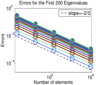
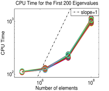
Figure 1: The errors and CPU time (in second) of the parallel augmented subspace method for the first 200 eigenpairs of Example 1.

From Figure 1, we can find that Algorithm 2 has the optimal error estimate, and needs similar computational work for different eigenpair. Here, the optimal error estimate means the concerned eigenvalue approximations have the errors which are bounded by the discretization errors of the finite element method on the corresponding level of meshes.

We also test the algebraic errors $|\bar{\lambda}_{i,h_{n}}-\lambda_{i,h_{n}}|$ between the numerical approximations by Algorithm 2 and the exact finite element solutions for the first $20$ eigenvalues on the finest level of mesh. The corresponding results are presented in Figure 2 which shows that the algebraic accuracy improves along with the growth of numbers of correction steps $\varpi_{n}$.

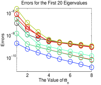
Figure 2: The algebraic errors for the first 20 eigenvalues of Example 1 by the parallel augmented subspace method with different number of correction steps.

The performance of Algorithm 2 for computing the first $1000$ eigenpairs is also investigated. Figure 3 shows the error estimate and CPU time for each eigenvalue. From Figure 3, we can also find the parallel method has optimal convergence order even for the first $1000$ eigenpairs. These results show the efficiency of Algorithm 2 and validity of Theorem 3.3 and Corollary 3.1.

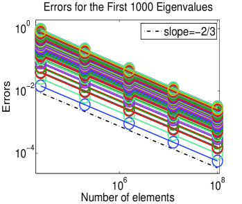
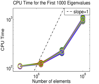
Figure 3: The errors and CPU time (in second) of the parallel augmented subspace method for the first 1000 eigenpairs of Example 1.

In order to check the orthogonality of approximate eigenfunctions by Algorithm 2, we investigate the inner products of eigenfunctions corresponding to different eigenvalues. We compute inner products for the first $100$ approximate eigenfunctions on the finest level of mesh by Algorithm 2. Figure 4 shows the biggest values of inner product of eigenfunctions according to different eigenvalues along with the growth of correction steps on the finest level of mesh. The results in Figure 4 show that Algorithm 2 can keep the orthogonality when the algebraic accuracy is small enough, which validates Remark 3.2.

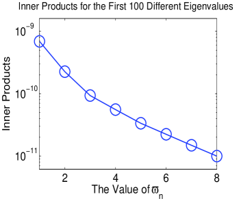
Figure 4: The inner products of the eigenfunctions corresponding to the first 100 different eigenvalues of Example 1.

5.2 A more general eigenvalue problem

In this example, we consider the following second order elliptic eigenvalue problem: Find $(\lambda,u)\in\mathcal{R}\times V$ such that $\|u\|_{a}=1$ and

$$\left\{\begin{array}[]{rcl}-\nabla\cdot(\mathcal{A}\nabla u)+\varphi u&=&\lambda u\ \ \ {\rm in}\ \Omega,\\ u&=&0\ \ \ \ \ {\rm on}\ \partial\Omega,\\ \|u\|_{0,\Omega}&=&1,\end{array}\right.$$ (5.4)

where

$$\mathcal{A}=\left(\begin{array}[]{ccc}$$1+(x_{1}-\frac{1}{2})^{2}$$&$$(x_{1}-\frac{1}{2})(x_{2}-\frac{1}{2})$$&$$(x_{1}-\frac{1}{2})(x_{3}-\frac{1}{2})$$\\ $$(x_{1}-\frac{1}{2})(x_{2}-\frac{1}{2})$$&$$1+(x_{2}-\frac{1}{2})^{2}$$&$$(x_{2}-\frac{1}{2})(x_{3}-\frac{1}{2})$$\\ $$(x_{1}-\frac{1}{2})(x_{3}-\frac{1}{2})$$&$$(x_{2}-\frac{1}{2})(x_{3}-\frac{1}{2})$$&$$1+(x_{3}-\frac{1}{2})^{2}$$\end{array}\right),$$

$\varphi=e^{(x_{1}-\frac{1}{2})(x_{2}-\frac{1}{2})(x_{3}-\frac{1}{2})}$ and $\Omega=(0,1)\times(0,1)\times(0,1)$.

In order to check the parallel property of Algorithm 2, we compute the first $200$ eigenpairs of (5.4). Here, we choose $H=1/16$, $\beta=2$, $\varpi=\varpi_{n}=1$ and $n=5$. In the first step of one correction step defined by Algorithm 1, $1$ multigrid step with $2$ CG steps for pre- and post-smoothing is adopted to solve the linear problem (3.6). Since the exact solutions are not known, the adequate accurate approximations are chosen as the exact solutions for our numerical test. Figure 5 shows the corresponding error estimates of $|\lambda_{i}-\lambda_{i,h_{n}}|$ for $i=1,\cdots,200$ and the CPU time for each eigenpair, respectively. From Figure 5, we can find that Algorithm 2 has the optimal error estimate, and needs similar computational work for computing different eigenpair.

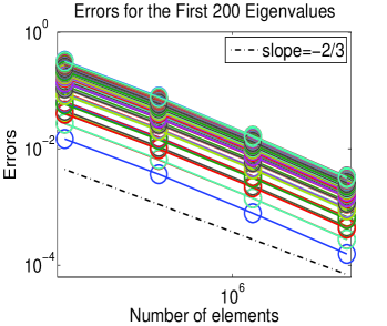
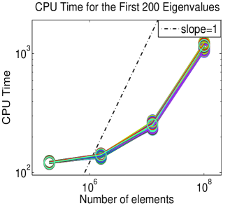
Figure 5: The errors and CPU time (in second) of the parallel augmented subspace method for the first 200 eigenpairs of Example 2.

In this example, we also test the algebraic error $|\bar{\lambda}_{i,h_{n}}-\lambda_{i,h_{n}}|$ between the numerical approximations by Algorithm 2 and the exact finite element solutions for the first $20$ eigenvalues along with the growth of the number of correction steps. The corresponding results are presented in Figure 6, which shows that the algebraic accuracy improves along with the growth of $\varpi_{n}$.

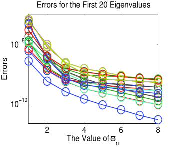
Figure 6: The algebraic errors for the first 20 eigenvalues of Example 2 by the parallel augmented subspace method with different number of correction step times.

Then, we compute the first $1000$ eigenpairs. The corresponding error estimates for the approximate eigenvalues and CPU time for each eigenpair are shown in Figure 7. From Figure 7, we can also find that the parallel method can arrive the theoretical convergence order for the first $1000$ eigenpairs. These results show the efficiency of Algorithm 2 and the validity of Theorem 3.3 and Corollary 3.1.

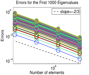
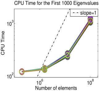
Figure 7: The errors and CPU time (in second) of the parallel augmented subspace method for the first 1000 eigenpairs of Example 2.

The orthogonality of approximate eigenfunctions by Algorithm 2 is also tested. In Figure 8, we also show the biggest values of inner product for the first $100$ approximate eigenfunctions according to different eigenvalues on the finest level of mesh. Form Figure 8, it can be found that Algorithm 2 can keep the orthogonality when the algebraic accuracy is small enough.

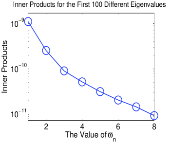
Figure 8: The inner products of the eigenfunctions corresponding to the first 100 different eigenvalues of Example 2.

5.3 Adaptive finite element method

In this example, we consider the following eigenvalue problem (see [15]): Find $(\lambda,u)\in\mathcal{R}\times V$ such that $\|u\|_{a}=1$ and

$$-\frac{1}{2}\Delta u+\frac{1}{2}|x|^{2}u=\lambda u\ \ \ {\rm in}\ \Omega,$$ (5.5)

where $\Omega=\mathcal{R}^{3}$ and $|x|=\sqrt{x_{1}^{2}+x_{2}^{2}+x_{3}^{2}}$. The eigenvalues of (5.5) are

$$\lambda_{i,j,k}=i+j+k+\frac{3}{2},$$

where $i,j,k$ denote the integral numbers and $i,j,k\geq 0$. Since the eigenfunctions are exponential decay, we set $\Omega=(-4,4)^{3}$ and the boundary condition $u=0\ {\rm on}\ \partial\Omega$ in our computation for simplicity. Since the exact eigenfunction with singularities is expected, the adaptive refinement is adopted to couple with Algorithm 2 (cf. [19]).

In order to check the parallel property of Algorithm 2, we compute the first $200$ eigenpairs of (5.5). In this example, we choose $H=1/4$, $\varpi=\varpi_{n}=1$. In the first step of one correction step defined by Algorithm 1, $1$ multigrid step with $2$ CG steps for pre- and post-smoothing is adopted to solve the linear problem (3.6). Figure 9 shows the corresponding error estimates of $|\lambda_{i}-\lambda_{i,h_{n}}|$ for $i=1,\cdots,200$ and the CPU time for each eigenpair. From Figure 9, we can find that Algorithm 2 has the optimal error estimates and needs similar computational work for different eigenvalue even on the adaptively refined meshes. These results show that Algorithm 2 can be coupled with the adaptive refinement technique.

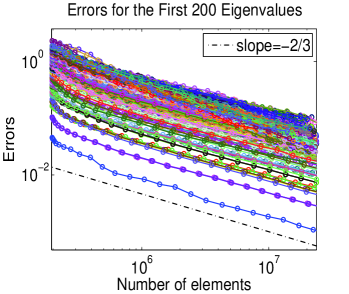
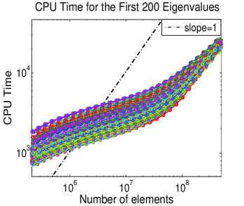
Figure 9: The errors and CPU time (in second) of the parallel augmented subspace method for the first 200 eigenvalues of Example 3.

5.4 Adaptive finite element method for Hydrogen atom

In order to show the potential for electrical structure simulation, in the last example, we consider the following model for Hydrogen atom: Find $(\lambda,u)\in\mathcal{R}\times V$ such that $\|u\|_{a}=1$ and

$$-\frac{1}{2}\Delta u-\frac{1}{|x|}u=\lambda u,\quad{\rm in}\ \Omega,$$ (5.6)

where $\Omega=\mathcal{R}^{3}$. The eigenvalues of (5.6) are $\lambda_{h}=-\frac{1}{2n^{2}}$ with multiplicity $n^{2}$ for any positive integer $n$. Along with the growths of $n$, it is easy to find that the spectral gap becomes small and the multiplicity large which improve the difficulty for solving the eigenvalue problem. The aim of this example is to show the parallel augmented subspace method in this paper can also compute the cluster eigenvalues and their eigenfunctions. Since the eigenfunction is exponential decay, we also set $\Omega=(-4,4)^{3}$ and the boundary condition $u=0$ on $\partial\Omega$ in our computation. Here the adaptive refinement is also adopted to couple with Algorithm 2.

In order to check the parallel property of Algorithm 2, we compute the first $200$ eigenpairs of (5.6). In this example, we choose $H=1/4$, $\varpi=\varpi_{n}=1$. In the first step of one correction step defined by Algorithm 1, $1$ multigrid step with $2$ CG steps for pre- and post-smoothing is adopted to solve the linear problem (3.6). Figure 10 shows the corresponding error estimates of $|\lambda_{i}-\lambda_{i,h_{n}}|$ for $i=1,\cdots,200$ and the CPU time for each eigenpair. From Figure 10, we can also find that Algorithm 2 has the optimal error estimate and needs similar computational work for different eigenvalue.

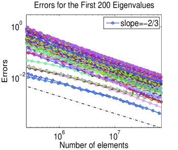
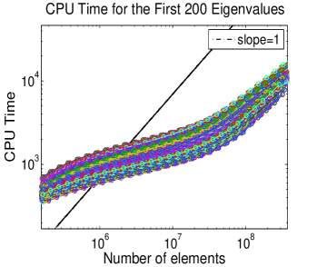
Figure 10: The errors and CPU time (in second) of the parallel augmented subspace method for the first 200 eigenvalues of Example 4.

6 Concluding remarks

In this paper, we propose a parallel augmented subspace scheme for eigenvalue problems by using the coarse space from the multigrid method. In this numerical method, solving the eigenvalue problem in the finest space is decomposed into solving the standard linear boundary value problems and very low dimensional eigenvalue problems. Furthermore, for different eigenvalue, the corresponding boundary value problem and low dimensional eigenvalue problem can be solved in the parallel way since they are independent of each other and there exists no data exchanging. This property means that we do not need to do the orthogonalization in the highest dimensional space and the the efficiency and scalability can be improved obviously.

The method in this paper can be applied to other types of linear and nonlinear eigenvalue problems such as biharmonic eigenvalue problem, Steklov eigenvalue problem, Kohn-Sham equation. These will be our future work.

References

- [1] R. A. Adams, Sobolev Spaces, Academic Press, New York, 1975.
- [2] I. Babuška and J. Osborn, Finite element-Galerkin approximation of the eigenvalues and eigenvectors of selfadjoint problems, Math. Comp., 52 (1989), 275–297.
- [3] I. Babuška and J. Osborn, Eigenvalue Problems, In Handbook of Numerical Analysis, Vol. II, (Eds. P. G. Lions and Ciarlet P.G.), Finite Element Methods (Part 1), North-Holland, Amsterdam, 641–787, 1991.
- [4] Z. Bai, J. Demmel, J. Dongarra, A. Ruhe, and H. van der Vorst, editors. Templates for the Solution of Agebraic Eigenvalue Problems: A Practical Guide, Society for Industrial and Applied Math., Philadelphia, 2000.
- [5] R. E. Bank and T. Dupont, An optimal order process for solving finite element equations, Math. Comp., 36 (1981), 35–51.
- [6] J. H. Bramble, Multigrid Methods, Pitman Research Notes in Mathematics, V. 294, John Wiley and Sons, 1993.
- [7] J. H. Bramble and J. E. Pasciak, New convergence estimates for multigrid algorithms, Math. Comp., 49 (1987), 311–329.
- [8] J. H. Bramble, J. Pasciak, and A. Knyazev, A subspace preconditioning algorithm for eigenvector/eigenvalue computation, Advances in Computational Mathematics, 6(1) (1996), 159–189.
- [9] J. H. Bramble and X. Zhang, The Analysis of Multigrid Methods, Handbook of Numerical Analysis, Vol. VII, P. G. Ciarlet and J. L. Lions, eds., Elsevier Science, 173–415, 2000.
- [10] S. Brenner and L. Scott, The Mathematical Theory of Finite Element Methods, New York: Springer-Verlag, 1994.
- [11] F. Chatelin, Spectral Approximation of Linear Operators, Academic Press Inc, New York, 1983.
- [12] H. Chen, H. Xie and F. Xu, A full multigrid method for eigenvalue problems, J. Comput. Phys., 322 (2016), 747–759.
- [13] P. G. Ciarlet, The finite Element Method for Elliptic Problem, North-holland Amsterdam, 1978.
- [14] E. G. D’yakonov and M. Yu. Orekhov, Minimization of the computational labor in determining the first eigenvalues of differential operators, Math. Notes, 27 (1980), 382–391.
- [15] W. Greiner, Quantum Mechanics: An Introduction, 3rd edn, Springer, Berlin, 1994.
- [16] W. Hackbusch, On the computation of approximate eigenvalues and eigenfunctions of elliptic operators by means of a multi-grid method, SIAM J. Numer. Anal., 16(2) (1979), 201–215.
- [17] W. Hackbusch, Multi-grid Methods and Applications, Springer-Verlag, Berlin, 1985.
- [18] V. Hernandez, J. E. Roman and V. Vidal, SLEPc: A scalable and flexible toolkit for the solution of eigenvalue problems, ACM Trans. Math. Software, 31(3) (2005), 351–362.
- [19] Q. Hong, H. Xie and F. Xu, A multilevel correction type of adaptive finite element method for eigenvalue problems, SIAM J. Sci. Comput.,, 40(6) (2018), A4208–A4235.
- [20] A. Knyazev, Preconditioned eigensolvers-an oxymoron? Electronic Transactions on Numerical Analysis, 7 (1998), 104–123.
- [21] A. Knyazev, Toward the optimal preconditioned eigensolver: Locally optimal block preconditioned conjugate gradient method, SIAM Journal on Scientific Computing, 23(2) (2001), 517–541.
- [22] A. V. Knyazev, M. E. Argentati, I. Lashuk and E. E. Ovtchinnikov, Block locally optimal preconditioned eigenvalue xolvers (BLOPEX) in hypre and PETSc, SIAM J. Sci. Comput., 29(5) (2007), 2224–2239.
- [23] A. Knyazev and K. Neymeyr, Efficient solution of symmetric eigenvalue problems using multigrid preconditioners in the locally optimal block conjugate gradient method, Electronic Transactions on Numerical Analysis., 15 (2003), 38–55.
- [24] Q. Lin and H. Xie, A multi-level correction scheme for eigenvalue problems, Math. Comp., 84 (2015), 71–88.
- [25] S. F. McCormick, ed., Multigrid Methods. SIAM Frontiers in Applied Matmematics 3. Society for Industrial and Applied Mathematics, Philadelphia, 1987.
- [26] Y. Saad, Numerical Methods For Large Eigenvalue Problems, Society for Industrial and Applied Mathematics, 2011.
- [27] L. R. Scott and S. Zhang, Higher dimensional non-nested multigrid methods, Math. Comp., 58 (1992), 457–466.
- [28] V. V. Shaidurov, Multigrid methods for finite element, Kluwer Academic Publics, Netherlands, 1995.
- [29] D. Sorensen, Implicitly Restarted Arnoldi/Lanczos Methods for Large Scale Eigen value Calculations, Springer Netherlands, 1997.
- [30] G. Strang and G. J. Fix, An Analysis of the Finite Element Method, Prentice-Hall, Eiglewood Cliffs, NJ, 1973.
- [31] A. Toselli and O. Widlund, Domain Decomposition Methods: Algorithm and Theory, Springer-Verlag, Berlin Heidelberg, 2005.
- [32] H. Xie, A type of multilevel method for the Steklov eigenvalue problem, IMA J. Numer. Anal., 34 (2014), 592–608.
- [33] H. Xie, A multigrid method for eigenvalue problem, J. Comput. Phys., 274 (2014), 550–561.
- [34] H. Xie, L. Zhang and H. Owhadi, Fast eigenvalue computation with operator adapted wavelets and hierarchical subspace correction, SIAM J. Numer. Anal, 57(6) (2019), 2519–2550.
- [35] J. Xu, Iterative methods by space decomposition and subspace correction, SIAM Review, 34(4) (1992), 581–613.
- [36] J. Xu, A new class of iterative methods for nonselfadjoint or indefinite problems, SIAM J. Numer. Anal., 29 (1992), 303–319.