Exact solutions in quantum field theory under rotation

Abstract

We discuss the construction and properties of rigidly-rotating states for free scalar and fermion fields in quantum field theory. On unbounded Minkowski space-time, we explain why such states do not exist for scalars. For the Dirac field, we are able to construct rotating vacuum and thermal states, for which expectation values can be computed exactly in the massless case. We compare these quantum expectation values with the corresponding quantities derived in relativistic kinetic theory.

1 Introduction

Rigidly-rotating systems are useful toy models for studying the underlying physics of more complex rotating systems in either flat or curved space-times. Consider a rigidly-rotating system of classical particles in flat space-time, rotating about a common axis, which we take to be the $z$-axis in the usual Cartesian coordinates. Assuming that the particles undergo circular motion with constant angular speed $\Omega$ about the rotation axis, the linear speed of each particle is then $\rho\Omega$, where $\rho$ is the distance of the particle from the axis of rotation. The speed of the particle therefore increases as the distance from the axis increases, and will become relativistic sufficiently far from the axis. Furthermore, if $\rho$ is sufficiently large, the particle will have a speed greater than the speed of light. Therefore a simple rigidly-rotating system cannot be realized in nature (at least in flat space-time), and the system must either be bounded in some way to prevent superluminal speeds, or else the system cannot be rigidly-rotating.

Although unbounded rigidly-rotating systems cannot be realized in flat space-time, nonetheless the study of rigidly-rotating systems in both relativistic kinetic theory (RKT) and quantum field theory (QFT) has a long history. The simplicity of the system allows many quantities of physical interest (such as quantum expectation values) to be computed exactly, which enables the extraction of the underlying physics. Many deep physical properties of rotating systems have been revealed by this approach, and in this chapter we outline some of the most important.

Our motivation for studying rigidly-rotating systems in QFT comes from both astrophysics and heavy ion collisions. In astrophysics, rigid rotation can be induced near rapidly-rotating magnetars or in accretion disks around black holes, where the field close to the surface of the star is sufficiently strong to lock charged particles into magnetically dominated accretion flow. The superluminal motion of the plasma constituents can be prohibited by the bending of the magnetic field lines far from the axis of rotation Meier:2012 . Particle geodesics on rotating black hole space-times also exhibit rigid rotation close to the event horizon due to the frame-dragging effect Chandrasekhar:1985kt . Quantum effects are important for black holes, which emit thermal quantum radiation Hawking:1974sw . Whether or not it is possible to define a quantum state representing a quantum field in thermal equilibrium with a rotating black hole depends on whether one considers a scalar field (in which case such a state does not exist Frolov:1989 ; Kay:1988mu ) or a fermion field (where a state can be constructed, but is divergent far from the black hole Casals:2013 ).

In the context of strongly interacting systems, rigid rotation can occur in the quark-gluon plasma (QGP) formed in the early stages following the collision of (ultra-)relativistic heavy ions Jacak:2012 . Just as a magnetic field can induce a charge current along the magnetic field direction in fermionic matter through the chiral magnetic effect, rigid rotation can induce an axial current through an analogous chiral vortical effect (CVE) Kharzeev:2016 . Due to the latter, the rotating fluid becomes polarised along the rotation axis. This polarisation was recently demonstrated through measurements of the properties of the decay products of $\Lambda$-hyperons STAR:2017 ; STAR:2018 . Interest in studying the properties of rigidly-rotating quantum systems has surged in the past few years, with recent studies addressing the hydrodynamic description of fluids with spin Florkowski:2018 , the role of the spin tensor in nonequilibrium thermodynamics Becattini:2019 and the properties of thermodynamic equilibrium for the free Dirac field with axial chemical potential Buzzegoli:2018 .

Our focus on this chapter is rigidly-rotating systems in flat-space QFT. We consider the simplest types of quantum field, namely a free scalar or Dirac fermion field. By ignoring the self-interactions of the quantum field, and the curvature of space-time, we are able to study in detail the effect of rotation alone. The construction of rotating vacuum and thermal states for these fields is compared with the corresponding construction of nonrotating vacuum and thermal states. Here the difference between bosonic and fermionic quantum fields play a major role. Having constructed the rotating states, we then elucidate their physical properties by studying, for the fermion field, the expectation values of the fermion condensate (FC), charge current (CC), axial current (AC), and stress-energy tensor (SET). We compare these with the analogous quantities computed within the framework of RKT, to elucidate the effects of quantum corrections.

This chapter is structured as follows. The problem of rigid rotation at finite temperature is addressed from an RKT perspective in section 2. Section 3 considers the construction of rigidly-rotating states in QFT, showing in particular that these states do not exist for a free quantum scalar field on unbounded flat space-time. The rest of the chapter is therefore devoted to the free Dirac field only. Mode solutions of the Dirac equation are derived with respect to a cylindrical coordinate system in section 4. We briefly consider nonrotating thermal expectation values (t.e.v.s) in section 5, and demonstrate that there are no quantum corrections for these states. On the other hand, for rotating states, the t.e.v.s constructed in section 6 are modified in QFT compared to the RKT results. We examine the physical properties of these quantum corrections for the SET in particular in section 7. The above discussion has focussed on unbounded flat space-time, and we briefly review some more general scenarios in section 8 before presenting our conclusions in section 9.

2 Relativistic kinetic theory

Before we address the properties of rigidly-rotating systems in QFT, we first consider the RKT perspective. We briefly describe the main features of a distribution of Bose-Einstein or Fermi-Dirac particles in global thermal equilibrium (GTE) undergoing rigid rotation.

2.1 Rigidly-rotating thermal distribution

Consider particles of mass $M$ and four-momentum $p^{\mu}$ in GTE in the absence of external forces. The configuration of particles is described by the distribution function $f$, which satisfies the relativistic Boltzmann equation Cercignani:2002

$$p^{\mu}\partial_{\mu}f={\mathcal{C}}[f],$$ (1)

using Cartesian coordinates on Minkowski space-time, so that $x^{\mu}=(t,x,y,z)^{T}$. In (1), ${\mathcal{C}}[f]$ is the collision operator, which drives the fluid towards local thermal equilibrium and whose properties give the form of the equilibrium distribution function. For neutral scalar particles, the equilibrium is described by the Bose-Einstein distribution function

$$f_{{\rm{S}}}=\frac{g_{\rm{S}}}{\left(2\pi\right)^{3}}\left[\exp\left(p_{\lambda}\beta^{\lambda}\right)-1\right]^{-1},$$ (2)

where $g_{\rm{S}}$ is the number of bosonic degrees of freedom and $\beta^{\mu}=u^{\mu}/T$ is the four-temperature, with $T$ the local temperature and $u^{\mu}$ the four-velocity. For simplicity, we do not include a chemical potential in the scalar case. The Fermi-Dirac distribution function, including a local chemical potential $\mu$ is

$$f_{\rm{F}}=\frac{g_{\rm{F}}}{(2\pi)^{3}}\left[\exp\left(p_{\lambda}\beta^{\lambda}-\mu/T\right)+1\right]^{-1},$$ (3)

where $g_{\rm{F}}$ is a degeneracy factor taking into account internal degrees of freedom, such as spin and colour charge.

GTE is achieved when the distribution function (2, 3) satisfies the Boltzmann equation (1). The fluid can be in GTE only when

$$\partial_{\lambda}(\mu/T)=0,\qquad\partial_{\lambda}\beta_{\kappa}+\partial_{\kappa}\beta_{\lambda}=0.$$ (4)

The first equality implies that, in the fermion case, the chemical potential is proportional to the temperature. The second equation requires that the four-temperature $\beta^{\mu}$ is a Killing vector. For Minkowski space-time, the general solution of the Killing equation allows $\beta_{\mu}$ to be written in the form:

$$\beta_{\mu}=b_{\mu}+\varpi_{\mu\nu}x^{\nu},$$ (5)

where the four-vector $b^{\mu}$ and the thermal vorticity tensor $\varpi_{\mu\nu}=-\frac{1}{2}(\partial_{\mu}\beta_{\nu}-\partial_{\nu}\beta_{\mu})$ are constants in GTE.

In order to describe a state of rigid rotation with angular velocity $\bm{\Omega}=\Omega\bm{k}$ about the $z$-axis, the constants appearing in (5) can be taken to be:

$$b^{\mu}=T_{0}^{-1}\delta^{\mu}{}_{0},\qquad\varpi_{\mu\nu}=\Omega T_{0}^{-1}\left(\eta_{\mu x}\eta_{\nu y}-\eta_{\mu y}\eta_{\nu x}\right),$$ (6)

where $\eta_{\mu\nu}={\rm{diag}}(1,-1,-1,-1)$ is the usual Minkowski metric. These values correspond to the four-temperature $\beta^{\mu}=T^{-1}_{0}(1,-\Omega y,\Omega x,0),$ where the physical interpretation of the constant $T_{0}$ is discussed below. Since the rigidly-rotating state is invariant under rotations about the $z$-axis, it is convenient to employ cylindrical coordinates $x^{\mu}=(t,\rho,\varphi,z)$ to refer to various vector or tensor components. Using the standard transformation formulae for vector components yields:

$$\beta^{t}=T_{0}^{-1},\qquad\beta^{\rho}=0,\qquad\beta^{\varphi}=\Omega T_{0}^{-1},\qquad\beta^{z}=0.$$ (7)

In our later discussion, it will prove useful to express vector and tensor components of physical quantities relative to an orthonormal (non-holonomic) tetrad $\{e_{\hat{\alpha}}\}$ consisting of four mutually orthogonal vectors of unit norm, $e_{\hat{\alpha}}=e_{\hat{\alpha}}^{\mu}\partial_{\mu}$, defined as:

$$e_{\hat{t}}=\partial_{t},\qquad e_{\hat{\rho}}=\partial_{\rho},\qquad e_{\hat{\varphi}}=\rho^{-1}\partial_{\varphi},\qquad e_{\hat{z}}=\partial_{z},$$ (8)

which satisfy the orthogonality relation:

$$g_{\mu\nu}e^{\mu}_{\hat{\alpha}}e^{\nu}_{\hat{\sigma}}=\eta_{\hat{\alpha}\hat{\sigma}},$$ (9)

where $g_{\mu\nu}={\rm diag}(1,-1,-\rho^{2},-1)$ is the metric tensor of Minkowski space-time with respect to the cylindrical coordinates.

Writing the four-temperature (7) with respect to the tetrad (8) yields the tetrad components:

$$\beta^{\hat{\alpha}}=\eta^{\hat{\alpha}{\hat{\sigma}}}e_{\hat{\sigma}}^{\mu}\beta_{\mu}=T_{0}^{-1}(1,0,\rho\Omega,0).$$ (10)

The squared norm of the above expression can be obtained using either the coordinate components $\beta^{\mu}$ or the tetrad components $\beta^{\hat{\alpha}}$, as follows:

$$\beta^{2}=g_{\mu\nu}\beta^{\mu}\beta^{\nu}=\eta_{\hat{\alpha}\hat{\sigma}}\beta^{\hat{\alpha}}\beta^{\hat{\sigma}}=T_{0}^{-2}(1-\rho^{2}\Omega^{2}).$$ (11)

Since $\beta^{\hat{\alpha}}=u^{\hat{\alpha}}/T$ and the four-velocity $u^{\hat{\alpha}}$ has unit norm by definition, it can be seen that the quantity $\sqrt{\beta^{2}}$ is the local inverse temperature $T^{-1}$. For a rigidly rotating system, the four-velocity has the tetrad components:

$$u^{\hat{\alpha}}=\Gamma(1,0,v^{\hat{\varphi}},0),$$ (12)

where we find the following relations:

$$T=T_{0}\Gamma,\qquad v^{\hat{\varphi}}=\rho\Omega,\qquad\Gamma=(1-\rho^{2}\Omega^{2})^{-1/2},$$ (13)

where $T$ is the local temperature. Equation (13) shows that $T_{0}$ is the temperature on the rotation axis and away from the axis the local temperature increases linearly with the Lorentz factor $\Gamma$ characterising the rigid rotation. Furthermore, we can readily identify the speed-of-light surface (SLS), which is the surface where the fluid rotates at the speed of light:

$$\rho_{\rm SLS}=\Omega^{-1}.$$ (14)

As expected, the Lorentz factor $\Gamma$ diverges on the SLS, and so does the local temperature $T$. Starting from the velocity field in (12), it is possible to compute the kinematic vorticity, $\omega^{\hat{\alpha}}=\frac{1}{2}\varepsilon^{\hat{\alpha}\hat{\beta}\hat{\gamma}\hat{\sigma}}u_{\hat{\beta}}\nabla_{\hat{\gamma}}u_{\hat{\sigma}}$, acceleration, $a^{\hat{\alpha}}=u^{\hat{\beta}}\nabla_{\hat{\beta}}u^{\hat{\alpha}}$ and circular vector $\tau^{\hat{\alpha}}=-\varepsilon^{\hat{\alpha}\hat{\beta}\hat{\gamma}\hat{\sigma}}\omega_{\hat{\beta}}a_{\hat{\gamma}}u_{\hat{\sigma}}$ Becattini:2015 ; Becattini:2015prd ; Ambrus:2019ayb ; Ambrus:2019khr :

$$\omega^{\hat{\alpha}}=\Gamma^{2}\Omega(0,0,0,1),\quad a^{\hat{\alpha}}=-\rho\Gamma^{2}\Omega^{2}(0,1,0,0),\quad\tau^{\hat{\alpha}}=-\rho\Omega^{3}\Gamma^{5}(\rho\Omega,0,1,0).$$ (15)

2.2 Macroscopic quantities

At sufficiently high temperatures, pair production processes can occur. It is thus necessary to account for the presence of both particle and anti-particle species. We consider only the simplest model. For the neutral scalar field in thermal equilibrium, particles and anti-particles have the same distribution function $f_{\rm{S}}$ (2). Fermions and anti-fermions are distributed according to the Fermi-Dirac distribution (3) at the same temperature $T$ and macroscopic velocity $u^{\hat{\alpha}}$, while the chemical potential is taken with the opposite sign for anti-particles:

$$f_{q/\overline{q}}=\frac{g_{\rm{F}}}{(2\pi)^{3}}\left[\exp(p_{\lambda}\beta^{\lambda}\mp\mu/T)+1\right]^{-1},$$ (16)

where $f_{q}$ is the distribution for fermions and $f_{\overline{q}}$ that for anti-fermions. For the rigidly-rotating system, the contraction of the four-temperature $\beta^{\mu}$ with the particle four-momentum is:

$$p_{\lambda}\beta^{\lambda}=T_{0}^{-1}\left[p^{t}-\bm{\Omega}\cdot(\bm{x}\times\bm{p})\right]=T_{0}^{-1}(p^{t}-\Omega M^{z})=T_{0}^{-1}{\widetilde{p}}^{t}$$ (17)

where $M^{z}$ denotes the $z$ component of the angular momentum, and we have defined the co-rotating energy ${\widetilde{p}}^{t}$ by

$$\widetilde{p}^{t}=p^{t}-\Omega M^{z}.$$ (18)

We first consider the zero temperature limit. From (2), it is clear that the scalar distribution function $f_{\rm{S}}\rightarrow 0$ as $T_{0}\rightarrow 0$, as expected. The situation is more complicated for the fermion distribution function (16), and depends on the sign of $p_{\lambda}\beta^{\lambda}\pm\mu/T$. Noting that $\mu/T=\mu_{0}/T_{0}$ (where $\mu_{0}$ is the chemical potential on the axis of rotation) is a constant from (4), the zero temperature limit of (16) is:

$$\lim_{T_{0}\rightarrow 0}f_{q/\overline{q}}=\frac{g_{\rm{F}}}{(2\pi)^{3}}\Theta(\pm{\mathcal{E}}_{F}-\widetilde{p}^{t}),\qquad$$ (19)

where ${\mathcal{E}}_{F}=\mu_{0}$ is the Fermi level and $\Theta$ is the Heaviside step function, equal to one when its argument is positive and zero otherwise. Thus, the particle/anti-particle distributions have non-vanishing values only when $\widetilde{p}^{t}<\mu_{0}$ for particles and $\widetilde{p}^{t}<-\mu_{0}$ for anti-particles.

Starting from the distribution functions, we can define the SET $T^{\hat{\alpha}\hat{\sigma}}_{\rm{S}/{\rm{F}}}$ for either a scalar or fermion field as follows:

$$T_{\rm{S}}^{\hat{\alpha}\hat{\sigma}}=\int\frac{d^{3}p}{p^{\hat{t}}}p^{\hat{\alpha}}p^{\hat{\sigma}}f_{S},\qquad T_{\rm{F}}^{\hat{\alpha}\hat{\sigma}}=\int\frac{d^{3}p}{p^{\hat{t}}}p^{\hat{\alpha}}p^{\hat{\sigma}}\left[f_{q}+f_{\overline{q}}\right].$$ (20)

For the fermion field, we can also define the macroscopic CC $J^{\hat{\alpha}}$:

$$J^{\hat{\alpha}}=\int\frac{d^{3}p}{p^{\hat{t}}}p^{\hat{\alpha}}[f_{q}-f_{\overline{q}}].$$ (21)

By construction, $J^{\hat{\alpha}}$ and $T^{\hat{\alpha}\hat{\sigma}}_{\rm{S}/{\rm{F}}}$ are space-time tensors. Due to the structure of the scalar and Fermi-Dirac distributions, the free indices of these quantities can be carried only by the Minkowski metric tensor $\eta^{\hat{\alpha}\hat{\beta}}$ or the macroscopic velocity $u^{\hat{\alpha}}$. These simple considerations immediately imply the perfect fluid form for the CC and SET:

$$J^{\hat{\alpha}}=Q_{{\rm{F}}}u^{\hat{\alpha}},\qquad T_{{\rm{S}}/{\rm{F}}}^{\hat{\alpha}\hat{\sigma}}=(E_{\rm{S}/{\rm{F}}}+P_{\rm{S}/{\rm{F}}})u^{\hat{\alpha}}u^{\hat{\sigma}}-P_{\rm{S}/{\rm{F}}}\eta^{\hat{\alpha}\hat{\sigma}},$$ (22)

where $Q_{\rm{F}}$ is the fermion charge density, $E_{\rm{S}/{\rm{F}}}$ is the energy density and $P_{\rm{S}/{\rm{F}}}$ is the pressure. An expression can be obtained for $Q_{\rm{F}}$ by contracting $J_{\rm{F}}^{\hat{\alpha}}$ with $u_{\hat{\alpha}}$. Similarly, $E_{\rm{S}/{\rm{F}}}$ is obtained by contracting $T_{\rm{S}/{\rm{F}}}^{\hat{\alpha}\hat{\sigma}}$ with $u_{\hat{\alpha}}u_{\hat{\sigma}}$, while a contraction of (22) with $\eta_{\hat{\alpha}\hat{\sigma}}$ yields the combination $E_{\rm{S}/{\rm{F}}}-3P_{\rm{S}/{\rm{F}}}$ on the right hand side. The above procedure applied to $Q_{\rm{F}}$ yields:

$$Q_{\rm{F}}=\frac{g_{\rm{F}}}{(2\pi)^{3}}\int\frac{d^{3}p}{p^{\hat{t}}}\left(u^{\lambda}p_{\lambda}\right)\left(\frac{1}{e^{\left(u^{\lambda}p_{\lambda}-\mu\right)/T}+1}-\frac{1}{e^{\left(u^{\lambda}p_{\lambda}+\mu\right)/T}+1}\right).$$ (23)

Taking advantage of the Lorentz invariance of the integration measure $d^{3}p/p^{\hat{t}}$, a Lorentz transformation can be performed on $p^{\lambda}$ such that $p^{\lambda}u_{\lambda}=p^{\hat{t}}$. Switching to spherical coordinates in momentum space, the integral over the angular coordinates is straightforward and gives

$$Q_{\rm{F}}=\frac{g_{\rm{F}}}{2\pi^{2}}\int_{0}^{\infty}dp\,p^{2}\left(\frac{1}{e^{\left(p^{\hat{t}}-\mu\right)/T}+1}-\frac{1}{e^{\left(p^{\hat{t}}+\mu\right)/T}+1}\right),$$ (24)

where $p=\left|{\bm{p}}\right|$ is the magnitude of the three-momentum. Similarly, we find, for the scalar field,

$$\begin{pmatrix}E_{\rm{S}}\\ E_{\rm{S}}-3P_{\rm{S}}\end{pmatrix}=\frac{g_{\rm{S}}}{2\pi^{2}}\int_{0}^{\infty}\frac{p^{2}dp}{p^{\hat{t}}}\begin{pmatrix}(p^{{\hat{t}}})^{2}\\ M^{2}\end{pmatrix}\frac{1}{e^{p^{\hat{t}}/T}-1},$$ (25)

while for the fermion field we have

$$\begin{pmatrix}E_{\rm{F}}\\ E_{\rm{F}}-3P_{\rm{F}}\end{pmatrix}=\frac{g_{\rm{F}}}{2\pi^{2}}\int_{0}^{\infty}\frac{p^{2}dp}{p^{\hat{t}}}\begin{pmatrix}(p^{\hat{t}})^{2}\\ M^{2}\end{pmatrix}\left(\frac{1}{e^{\left(p^{\hat{t}}-\mu\right)/T}+1}+\frac{1}{e^{\left(p^{\hat{t}}+\mu\right)/T}+1}\right).$$ (26)

Since the integrands above exhibit exponential decay at large values of $p$, they are amenable to numerical integration. The expressions (24, 25, 26) remain valid if the system is stationary rather than rotating, in which case $T=T_{0}$ and $\mu=\mu_{0}$ are constants.

In the massless limit, $p^{\hat{t}}=p$, $E_{\rm S/F}=3P_{\rm S/F}$ and the integrals in (24, 25, 26) can be performed analytically Jaiswal:2015mxa , giving the charge density $Q_{F}$ and pressures $P_{\rm S}$ and $P_{\rm F}$ as:

$$Q_{\rm{F}}=\frac{g_{\rm F}\mu}{6}\left(T^{2}+\frac{\mu^{2}}{\pi^{2}}\right),\quad P_{\rm{S}}=\frac{\pi^{2}g_{\rm{S}}T^{4}}{90},\quad P_{\rm{F}}=\frac{7\pi^{2}g_{\rm{F}}T^{4}}{360}+\frac{g_{\rm F}T^{2}\mu^{2}}{12}+\frac{g_{\rm F}\mu^{4}}{24\pi^{2}},$$ (27)

where $\mu=\mu_{0}\Gamma$ and $T=T_{0}\Gamma$. We also compute the massless limit of the ratio $T^{\mu}{}_{\mu}/M^{2}=(E-3P)/M^{2}$:

$$\lim_{M\rightarrow 0}\frac{E_{S}-3P_{S}}{M^{2}}=\frac{g_{\rm{S}}T^{2}}{12},\qquad\lim_{M\rightarrow 0}\frac{E_{F}-3P_{F}}{M^{2}}=\frac{g_{\rm{F}}T^{2}}{12}+\frac{g_{\rm F}\mu^{2}}{4\pi^{2}}.$$ (28)

The Lorentz factor $\Gamma$ (13) and thus $\mu$ and $T$ diverge as $\rho\rightarrow\Omega^{-1}$ and the SLS is approached. Therefore, for massless particles, all macroscopic quantities are divergent on the SLS. Including the chemical potential does not alter the rate at which the quantities diverge, but does increase their values on the axis of rotation.

To understand the effect of the particle mass, the integrals in (24, 25, 26) are performed numerically. The resulting quantities depend on the angular speed $\Omega$, the temperature on the axis $T_{0}$, the chemical potential on the axis $\mu_{0}$, the particle mass $M$, the distance from the axis $\rho$ and the numbers of degrees of freedom (dof) $g_{\rm{S}}$, $g_{\rm{F}}$. Here we consider values of these parameters which are pertinent for the QGP formed in heavy ion collisions. An analysis of the QGP fluid produced in accelerators indicates that it has the greatest vorticity of any fluid produced in a laboratory STAR:2017 ; Wang:2017 , with $\hbar\Omega\simeq 6.6\ {\rm MeV}$, where $\hbar$ is the reduced Planck’s constant. For this value of $\Omega$, the SLS is located at $c/\Omega\simeq 30\ {\rm{fm}}$, roughly twice the size of a gold nucleus. For the temperature, we consider a typical value for heavy ion collisions of $k_{\rm{B}}T_{0}\simeq 0.2\ {\rm GeV}$ STAR:2017 , where $k_{B}$ is the Boltzmann constant. In the relativistic collision of gold nuclei, a typical value of the chemical potential is $\mu_{0}\simeq 0.1\ {\rm GeV}$ Huang:2012 . For the particle mass $Mc^{2}$, we consider the pion mass ($0.140\ {\rm GeV}$), the $\rho$ meson mass ($0.775\ {\rm GeV}$), the $\Lambda^{0}$-hyperon mass ($1.116\ {\rm GeV}$) and the $\Lambda^{+}_{c}$-charmed hyperon mass ($2.286\ {\rm GeV}$) particlerev .

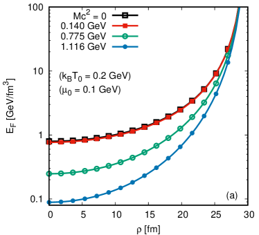
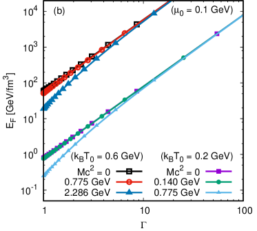
Figure 1: (a) Numerical results for the energy density $E_{F}$ (26), in ${\rm GeV}/{\rm fm}^{3}$ at $\mu_{0}=0.1\ {\rm GeV}$ and $k_{\rm{B}}T_{0}=0.2\ {\rm GeV}$, for $Mc^{2}=0$, $0.14\ {\rm GeV}$, $0.775\ {\rm GeV}$ and $1.116\ {\rm GeV}$. (b) Log-log plot of $E_{F}$, at two temperatures ($k_{\rm{B}}T_{0}=0.2\ {\rm GeV}$ and $0.6\ {\rm GeV}$), for various masses. The number of degrees of freedom was set to $g_{\rm{F}}=6$.

In figure 1 we plot the radial profile of the energy density $E_{\rm{F}}$ (26) as a function of $\rho$ (left-hand-plot, linear scale) and as a function of the Lorentz factor $\Gamma$ (13) (right-hand-plot, logarithmic scale). As expected, the energy diverges on the SLS for all values of the particle mass. The results for pions and massless particles are very nearly identical; for larger values of the mass the energy $E_{\rm{F}}$ is lower everywhere. However, close to the SLS the results for massive particles are indistinguishable from those for massless particles. Similar behaviour is observed for the pressure $P_{\rm{F}}$ and charge density $Q_{\rm{F}}$ Ambrus:2019ayb ; Ambrus:2019khr . This is in agreement with the analytic work in the zero chemical potential case Ambrus:2015 (see also Florkowski:2013 for details of relevant techniques), where it was found that the ${\mathcal{O}}(M^{2})$ corrections due to the mass make subleading contributions as the SLS is approached.

We now consider more closely the effect of varying the particle mass for both scalars and fermions. To make the comparison relevant, we consider the energy density per particle degree of freedom, which amounts to dividing $E_{\rm F}$ by $2g_{\rm{F}}$ (the factor of two is required since the particle and anti-particle states are explicitly taken into account) and $E_{\rm S}$ by $g_{\rm{S}}$. Furthermore, we consider the case of vanishing chemical potential, $\mu_{0}=0$, since we have not introduced this quantity for scalars.

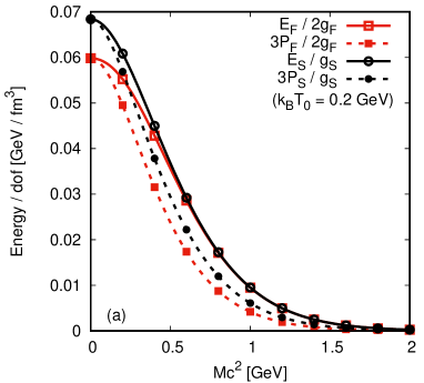
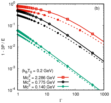
Figure 2: (a) The mass dependence of the energy (continuous lines and empty symbols) and pressure (dashed lines and filled symbols) per dof, computed for the Fermi-Dirac (squares) and Bose-Einstein (circle) statistics. (b) The dependence on the Lorentz factor $\Gamma$ (13) of the quantity $1-3P/E$, evaluated for the Fermi-Dirac (continuous lines and empty symbols) and Bose-Einstein (dashed lines and filled symbols) statistics, for various values of the particle mass.

Figure 2(a) shows the effect of the particle mass on the energy density and pressure on the rotation axis. For both scalars and fermions, these quantities decrease as the particle mass increases. In figure 2(b) we plot the quantity $1-3P/E$, which vanishes in the massless limit. For a constant value of the Lorentz factor $\Gamma$, we see that $1-3P/E$ increases as the mass is increased, thus the ratio $3P/E$ decreases. As the SLS is approached, $1-3P/E$ decreases, showing that in the vicinity of the SLS, the gas behaves as though its constituents were massless.

3 Quantum rigidly-rotating thermal states

We now consider the generalization from RKT to QFT, and examine how rigidly-rotating quantum states may be defined. In the quantization process, the microscopic momenta are promoted to quantum operators. Thermal states at a temperature $T_{0}$ are defined such that the t.e.v. of an operator ${\widehat{A}}$ takes the form Kapusta:1989 :

$$\braket{\widehat{A}}_{T_{0}}=Z^{-1}{\rm Tr}(\widehat{\rho}\widehat{A}),$$ (29)

where $Z={\rm{Tr}}{\widehat{\rho}}$ is the partition function and ${\widehat{\rho}}$ is the Boltzmann factor, which we define below. The trace is performed over Fock space, that is, the space of all states of the quantum field containing $n$ particles (or anti-particles), for $n=0,1,2,\ldots$.

For a rigidly-rotating state with temperature $T_{0}$ on the axis of rotation, the Boltzmann factor for a scalar field is given by Vilenkin:1980 :

$$\widehat{\rho}_{\rm{S}}=\exp\left[-(\widehat{H}_{\rm{S}}-\Omega\widehat{M}_{\rm{S}}^{z})/T_{0}\right],$$ (30)

where ${\widehat{H}}_{\rm{S}}$ is the scalar Hamiltonian operator and ${\widehat{M}}_{\rm{S}}^{z}$ is the $z$-component of the scalar angular momentum operator. For a fermion field, we include a chemical potential $\mu_{0}$ on the axis of rotation, which is conjugate to the charge operator. The Boltzmann factor for a fermion field is then given by Vilenkin:1980 :

$$\widehat{\rho}_{\rm{F}}=\exp\left[-(\widehat{H}_{\rm{F}}-\Omega\widehat{M}_{\rm{F}}^{z}-\mu_{0}\widehat{Q}_{\rm{F}})/T_{0}\right],$$ (31)

where $\widehat{H}_{\rm{F}}$ is the fermion Hamiltonian operator, $\widehat{M}_{\rm{F}}^{z}$ is the $z$-component of the total fermion angular momentum operator and $\widehat{Q}_{\rm{F}}$ is the fermion charge operator.

In order to perform the trace over Fock space in (29), we need to define particle creation and annihilation operators acting on the states. For a neutral scalar field, we denote the particle annihilation operators by ${\hat{a}}_{j}$, where $j$ labels the quantum properties of the annihilated particle. For a fermion field, the operators ${\hat{b}}_{j}$ annihilate fermions, while the ${\hat{d}}_{j}$ operators annihilate anti-fermions. In all cases, the adjoint operators are the corresponding particle creation operators. For scalars, the particle creation and annihilation operators satisfy the canonical commutation relations

$$[{\hat{a}}_{j},{\hat{a}}_{j^{\prime}}^{\dagger}]={\hat{a}}_{j}{\hat{a}}_{j^{\prime}}^{\dagger}-{\hat{a}}_{j^{\prime}}^{\dagger}{\hat{a}}_{j}=\delta_{j,j^{\prime}},\qquad[{\hat{a}}_{j},{\hat{a}}_{j^{\prime}}]=0=[{\hat{a}}_{j}^{\dagger},{\hat{a}}_{j^{\prime}}^{\dagger}],$$ (32)

where $\delta_{j,j^{\prime}}$ vanishes unless the labels $j$ and $j^{\prime}$ are identical. For fermions, canonical anti-commutation relations hold, so that, for the particle operators:

$$\{\hat{b}_{j},\hat{b}^{\dagger}_{j^{\prime}}\}=\hat{b}_{j}\hat{b}^{\dagger}_{j^{\prime}}+\hat{b}^{\dagger}_{j^{\prime}}\hat{b}_{j}=\delta_{j,j^{\prime}},\qquad\{\hat{b}_{j},\hat{b}_{j^{\prime}}\}=0=\{\hat{b}_{j}^{\dagger},\hat{b}^{\dagger}_{j^{\prime}}\},$$ (33)

and similar relations hold for the anti-particle operators.

Using the particle/anti-particle states corresponding to the above creation and annihilation operators, we consider a quantization which is compatible with the operator ${\widehat{\rho}}$, so that, for scalars:

$${\widehat{\rho}}_{\rm{S}}{\hat{a}}_{j}^{\dagger}\left({\widehat{\rho}}_{\rm{S}}\right)^{-1}=e^{-\left(E_{j}-\Omega m_{j}\right)/T_{0}}{\hat{a}}_{j}^{\dagger},$$ (34)

where $E_{j}$ is the energy of the created particle, and $m_{j}=0,\pm 1,\pm 2,\ldots$ is the $z$-component of the angular momentum. Similarly, for fermions we assume that

$$\widehat{\rho}_{\rm{F}}\hat{b}_{j}^{\dagger}\left(\widehat{\rho}_{\rm{F}}\right)^{-1}=e^{-\left(E_{j}-\Omega m_{j}-\mu_{0}\right)/T_{0}}\hat{b}_{j}^{\dagger},\qquad\widehat{\rho}_{\rm{F}}\hat{d}_{j}^{\dagger}\left(\widehat{\rho}_{\rm{F}}\right)^{-1}=e^{-\left(E_{j}-\Omega m_{j}+\mu_{0}\right)/T_{0}}\hat{d}_{j}^{\dagger},$$ (35)

where $m_{j}=\pm\frac{1}{2},\pm\frac{3}{2},\dots$ is the projection of the total fermion angular momentum on the $z$-axis. The quantities (34, 35) depend on the energy ${\widetilde{E}}_{j}$ of the particle as seen by a co-rotating observer:

$${\widetilde{E}}_{j}=E_{j}-\Omega m_{j}.$$ (36)

Using the canonical commutation/anti-commutation relations (32, 33), together with (34, 35), we find the t.e.v.s of the number operators for scalars to be Vilenkin:1980 ; Itzykson:1980rh :

$$\braket{{\hat{a}}^{\dagger}_{j}{\hat{a}}_{j^{\prime}}}_{T_{0}}=\frac{\delta_{j,j^{\prime}}}{\exp[{\widetilde{E}}_{j}/T_{0}]-1},$$ (37)

while for fermions we have

$$\braket{\hat{b}^{\dagger}_{j}\hat{b}_{j^{\prime}}}_{T_{0}}=\frac{\delta_{j,j^{\prime}}}{\exp[(\widetilde{E}_{j}-\mu_{0})/T_{0}]+1},\qquad\braket{\hat{d}^{\dagger}_{j}\hat{d}_{j^{\prime}}}_{T_{0}}=\frac{\delta_{j,j^{\prime}}}{\exp[(\widetilde{E}_{j}+\mu_{0})/T_{0}]+1}.$$ (38)

The t.e.v.s (37, 38) have the expected Bose-Einstein/Fermi-Dirac thermal distributions in terms of the co-rotating energy ${\widetilde{E}}_{j}$.

Consider first the scalar field t.e.v. (37). This has the correct zero-temperature limit only if ${\widetilde{E}}_{j}>0$. Even with this restriction, it can be seen that (37) diverges when ${\widetilde{E}}_{j}\rightarrow 0$, leading to the divergence of all t.e.v.s (29) Vilenkin:1980 ; Duffy:2002ss . From this we deduce that rigidly-rotating thermal states cannot be defined for a quantum scalar field on unbounded Minkowski space-time Vilenkin:1980 ; Duffy:2002ss ; Ambrus:2014uqa .

To understand this result, we consider how a quantum vacuum state is defined for a scalar field. In the canonical quantization approach to QFT, one starts with an orthonormal basis of scalar field modes $\phi_{j}$ which are solutions of the Klein-Gordon equation for a massive scalar field, $\left(\partial_{\mu}\partial^{\mu}+M^{2}\right)\phi_{j}=0$. The scalar field operator ${\widehat{\Phi}}$ is then written as a sum over these field modes and their complex conjugates

$${\widehat{\Phi}}=\sum_{j}\left[{\hat{a}}_{j}\phi_{j}+{\hat{a}}_{j}^{\dagger}\phi_{j}^{*}\right],$$ (39)

where the expansion coefficients are the particle creation and annihilation operators. In order that the creation and annihilation operators satisfy the canonical commutation relations (32), it must be the case that

$$\braket{\phi_{j},\phi_{j^{\prime}}}=\delta_{j,j^{\prime}},\qquad\braket{\phi^{*}_{j},\phi_{j^{\prime}}^{*}}=-\delta_{j,j^{\prime}},\qquad\braket{\phi_{j},\phi^{*}_{j^{\prime}}}=0,$$ (40)

where $\braket{\,,\,}$ is the Klein-Gordon inner product, defined for two solutions $\phi_{j}$, $\phi_{j^{\prime}}$ of the Klein-Gordon equation by the following integral over a constant-$t$ surface:

$$\braket{\phi_{j},\phi_{j^{\prime}}}=i\int d^{3}x\left(\phi_{j}^{*}\partial^{t}\phi_{j^{\prime}}-\phi_{j^{\prime}}\partial^{t}\phi_{j}^{*}\right).$$ (41)

In particular, the modes $\phi_{j}$ corresponding to particles must have positive norm $\braket{\phi_{j},\phi_{j}}$, while those modes $\phi_{j}^{*}$ corresponding to antiparticle modes must have negative norm. This restricts whether modes can be labelled as “particle” or “antiparticle”. Calculating the inner product for a particle mode with energy $E_{j}$, we find

$$\braket{\phi_{j},\phi_{j^{\prime}}}=\frac{E_{j}}{\left|E_{j}\right|}\delta_{j,j^{\prime}},$$ (42)

and hence the relations (40) hold only if the energy $E_{j}$ of the mode $\phi_{j}$ is positive, $E_{j}>0$ Letaw:1979wy . The vacuum state $|0\rangle$ is then defined as that state which is annihilated by the particle annihilation operators, ${\hat{a}}_{j}|0\rangle=0$, and is simply the (stationary) Minkowski vacuum. For a quantum scalar field, it is not possible to make the choice ${\widetilde{E}}_{j}>0$ because, for fixed ${\widetilde{E}}_{j}>0$, there will be modes with sufficiently large and negative $m_{j}$ for which $E_{j}={\widetilde{E}}_{j}+\Omega m_{j}<0$, so that (40) no longer holds and we do not have a valid quantization Letaw:1979wy . Since there is no rotating vacuum for a quantum scalar field, rotating thermal states for a quantum scalar field are also ill-defined.

One resolution of this difficulty is to insert a reflecting boundary inside the SLS Vilenkin:1980 ; Duffy:2002ss . The presence of the boundary means that the energy $E_{j}$ of the scalar field modes is quantized, and, if the boundary is inside the SLS, it can be shown that ${\widetilde{E}}_{j}>0$ for all $m_{j}$ Duffy:2002ss ; Nicolaevici:2001 . In this case a rotating vacuum state (and also rotating thermal states) can be defined for a quantum scalar field Duffy:2002ss .

In view of these difficulties for a quantum scalar field, for the rest of this chapter we restrict our attention to a quantum fermion field on unbounded Minkowski space-time. First we consider whether a rotating vacuum state can be defined in canonical quantization. Beginning with an orthonormal basis of particle mode solutions $U_{j}$ and anti-particle mode solutions $V_{j}$ of the Dirac equation (which will be discussed in more detail in the next section), the fermion field operator is written as

$${\widehat{\Psi}}=\sum_{j}\left[{\hat{b}}_{j}U_{j}+{\hat{d}}_{j}^{\dagger}V_{j}\right],$$ (43)

where the operators ${\hat{b}}_{j}$ and ${\hat{d}}_{j}$ satisfy the canonical anti-commutation relations (33). In contrast to the scalar field case, all particle and antiparticle modes $U_{j}$, $V_{j}$ have positive Dirac norm, resulting in a greater freedom to label modes as “particle” or “anti-particle”. This in turn leads to a greater freedom in how vacuum states (and therefore also thermal states) are defined Ambrus:2014uqa .

One possible quantization is to define “particle” modes as having positive energy $E_{j}$ Vilenkin:1980 . As in the scalar case, the resulting vacuum is simply the usual (nonrotating) Minkowski vacuum state. However, for fermions there is another possibility Iyer:1982ah : particle modes can be defined by setting ${\widetilde{E}}_{j}>0$. This leads to a well-defined quantization and a rotating vacuum state. Furthermore, with this definition the t.e.v.s (38) have the correct zero-temperature limit, with contributions only from modes below the Fermi level, for which $\widetilde{E}_{j}<\mu_{0}$ for particle modes and ${\widetilde{E}}_{j}<-\mu_{0}$ for antiparticle modes (we remind the reader that $\widetilde{E}_{j}>0$ always holds when the rotating vacuum is employed). This is in agreement with the corresponding result (19) in the RKT case, and is sufficient to ensure that there are no temperature- and chemical potential-independent contributions to t.e.v.s.

4 Mode solutions in cylindrical coordinates

Our purpose for the remainder of this chapter is to compute t.e.v.s of observables for a quantum fermion field of mass $M$, and compare the results with those for the RKT approach in section 2.2. In this section we lay the groundwork for our computation by considering in more detail the fermion mode solutions discussed schematically in the previous section. Since we are interested in rigidly-rotating states, we work in cylindrical coordinates $x^{\mu}=(t,\rho,\varphi,z)$ and follow the approach of Ambrus:2014uqa ; Ambrus:2015lfr .

The evolution of a free Dirac field with mass $M$ is governed by the least-action principle, starting from the action:

$$S_{\rm{F}}=i\int d^{4}x\,\mathcal{L},\qquad\mathcal{L}=\frac{i}{2}\left(\overline{\psi}\not{\partial}\psi-\overline{\not{\partial}\psi}\psi\right)-M\overline{\psi}\psi,$$ (44)

where the Feynman slash denotes contraction with the gamma matrices $\not{\partial}=\gamma^{\mu}\partial_{\mu}$. The gamma matrices satisfy the canonical anti-commutation relations $\{\gamma^{\mu},\gamma^{\nu}\}=2\eta^{\mu\nu}$ and in this chapter, we work with the Dirac representation:

$$\gamma^{t}=\begin{pmatrix}1&0\\ 0&-1\end{pmatrix},\qquad\gamma^{i}=\begin{pmatrix}0&\sigma^{i}\\ -\sigma^{i}&0\end{pmatrix},$$ (45)

where the Pauli matrices are given by:

$$\sigma^{x}=\begin{pmatrix}0&1\\ 1&0\end{pmatrix},\qquad\sigma^{y}=\begin{pmatrix}0&-i\\ i&0\end{pmatrix},\qquad\sigma^{z}=\begin{pmatrix}1&0\\ 0&-1\end{pmatrix}.$$ (46)

We are considering four-spinors $\psi$, which have Dirac adjoint ${\overline{\psi}}=\psi^{\dagger}\gamma^{t}$. Demanding that the variation of the action $S_{\rm{F}}$ (44) with respect to the $\overline{\psi}$ degree of freedom vanishes yields the Dirac equation

$$(i\not{\partial}-M)\psi=0.$$ (47)

As outlined in the previous section, in order to construct t.e.v.s we first require a set of particle modes $\{U_{j}\}$ and anti-particle modes $\{V_{j}\}$ satisfying the Dirac equation (47). Given a particle mode $U_{j}$, the corresponding anti-particle mode $V_{j}$ is related to $U_{j}$ by the charge conjugation operation:

$$V_{j}=i\gamma^{y}U_{j}^{*}.$$ (48)

In deriving the formal expressions for rigidly-rotating t.e.v.s in section 3, we have assumed a quantization compatible with ${\widehat{\rho}}$, see (35). This requires that the following commutation relations must hold:

$$[\widehat{H}_{\rm{F}},\hat{b}_{j}^{\dagger}]= E_{j}\hat{b}_{j}^{\dagger}, [\widehat{M}^{z}_{\rm{F}},\hat{b}_{j}^{\dagger}]= m_{j}\hat{b}_{j}^{\dagger}, [\widehat{Q}_{\rm{F}},\hat{b}_{j}^{\dagger}]= \hat{b}_{j}^{\dagger},$$

$$[\widehat{H}_{\rm{F}},\hat{d}_{j}^{\dagger}]= E_{j}\hat{d}_{j}^{\dagger}, [\widehat{M}^{z}_{\rm{F}},\hat{d}_{j}^{\dagger}]= m_{j}\hat{d}_{j}^{\dagger}, [\widehat{Q}_{\rm{F}},\hat{d}_{j}^{\dagger}]= -\hat{d}_{j}^{\dagger}.$$ (49)

Taking into account the expression for the conserved operators in the classical Dirac field theory,

$$H_{\rm{F}}=i\partial_{t},\qquad M^{z}_{\rm{F}}=-i\partial_{\varphi}+S^{z},$$ (50)

where the $z$-projection of the spin operator $S^{z}$ is given by:

$$S^{z}=\frac{1}{2}\begin{pmatrix}\sigma^{z}&0\\ 0&\sigma^{z}\end{pmatrix},$$ (51)

the particle mode solutions $U_{j}$ must thus be chosen to be simultaneous eigenfunctions of $H_{\rm{F}}$ and $M^{z}_{\rm{F}}$:

$$H_{\rm{F}}U_{j}=E_{j}U_{j},\qquad M^{z}_{\rm{F}}U_{j}=m_{j}U_{j}.$$ (52)

The above eigenvalue equations are insufficient to specify the particle mode solutions uniquely. The remaining degrees of freedom can be fixed by choosing $U_{j}$ to be eigenfunctions of the longitudinal momentum operator $P^{z}_{\rm{F}}=-i\partial_{z}$ and of the helicity operator $W_{0}=\bm{J}\cdot\bm{P}_{\rm{F}}/2p$ (where $p$ is the magnitude of the momentum):

$$P^{z}_{\rm{F}}U_{j}=k_{j}U_{j},\qquad W_{0}U_{j}=\lambda_{j}U_{j},$$ (53)

where $k_{j}$ and $\lambda_{j}$ are real constants. The expression for $W_{0}$ can be obtained as follows:

$$W_{0}=\begin{pmatrix}h&0\\ 0&h\end{pmatrix},\qquad h=\frac{\bm{\sigma}\cdot\bm{P}_{\rm{F}}}{2p}=\frac{1}{2p}\begin{pmatrix}P^{z}_{\rm{F}}&P_{-}\\ P_{+}&-P^{z}_{\rm{F}},\end{pmatrix},$$ (54)

where $\bm{P}_{\rm F}=-i\nabla$, while $P_{\pm}$ are defined in terms of cylindrical coordinates as:

$$P_{\pm}=P^{x}_{\rm{F}}\pm iP^{y}_{\rm{F}}=-ie^{\pm i\varphi}(\partial_{\rho}\pm i\rho^{-1}\partial_{\varphi}).$$ (55)

It can be shown that $W_{0}^{2}=\frac{1}{4}$. The eigenvalues $\lambda_{j}=1/2$ and $-1/2$ correspond to positive and negative helicity, respectively.

The Dirac equation (47) can be written with respect to the above operators as:

$$\begin{pmatrix}H_{\rm{F}}-M&-2ph\\ 2ph&-H_{\rm{F}}-M\end{pmatrix}\psi=0.$$ (56)

The operators $H_{\rm{F}}$ and $P^{z}_{\rm{F}}$ are diagonal with respect to the spinor structure, thus the corresponding eigenvalue equations can be solved immediately:

$$U_{j}=\frac{{\mathcal{K}}_{j}}{2\pi}e^{-iE_{j}t+ik_{j}z}u_{j},\qquad u_{j}=\begin{pmatrix}\mathcal{C}_{j}^{-}\phi_{j}\\ \mathcal{C}_{j}^{+}\phi_{j},\end{pmatrix},$$ (57)

where $u_{j}$ is a four-spinor which depends only on $\varphi$ and $\rho$ and ${\mathcal{K}}_{j}$ is a normalization constant. In (57), $\mathcal{C}_{j}^{\pm}$ are integration constants and $\phi_{j}$ is a two-spinor satisfying the remaining two eigenvalue equations, namely:

$$\left(-i\partial_{\varphi}+\frac{1}{2}\sigma^{z}\right)\phi_{j}=m_{j}\phi_{j},\qquad h\phi_{j}=\lambda_{j}\phi_{j}.$$ (58)

Substituting (57) into the Dirac equation (56) gives

$$\begin{pmatrix}E_{j}-M&-2p_{j}\lambda_{j}\\ 2p_{j}\lambda_{j}&-E_{j}-M\end{pmatrix}u_{j}=0,$$ (59)

where the magnitude of the momentum is now $p_{j}$, and from this the following relation can be established for $\mathcal{C}_{j}^{\pm}$:

$$\mathcal{C}_{j}^{-}=\frac{2\lambda_{j}p_{j}}{E_{j}-M}\mathcal{C}_{j}^{+}.$$ (60)

Next we consider the angular momentum equation, the first relation in (58), which allows $\phi_{j}$ to be written in the form:

$$\phi_{j}=\begin{pmatrix}\phi_{j}^{-}e^{i(m_{j}-\frac{1}{2})\varphi}\\ \phi_{j}^{+}e^{i(m_{j}+\frac{1}{2})\varphi}\end{pmatrix},$$ (61)

where $m_{j}=\pm\frac{1}{2},\pm\frac{3}{2},\dots$ is an odd half-integer, while $\phi_{j}^{\pm}\equiv\phi_{j}^{\pm}(\rho)$ are functions which depend only on the radial coordinate $\rho$. Taking into account the result [from (55)] $P_{+}P_{-}=P_{-}P_{+}=-\partial_{\rho}^{2}-\rho^{-1}\partial_{\rho}-\rho^{-2}\partial_{\varphi}^{2}$, the second relation in (58) reduces to:

$$\left[\rho^{2}\frac{\partial^{2}}{\partial\rho^{2}}+\rho\frac{\partial}{\partial\rho}+q_{j}^{2}\rho^{2}-\left(m_{j}\pm\frac{1}{2}\right)^{2}\right]\phi_{j}^{\pm}=0,$$ (62)

where the longitudinal momentum $q_{j}$ is defined by

$$q_{j}=\sqrt{p_{j}^{2}-k_{j}^{2}}=\sqrt{E_{j}^{2}-k_{j}^{2}-M^{2}}.$$ (63)

Equation (62) can readily be identified with the Bessel equation Olver:2010 , having two linearly independent solutions $J_{m\pm 1/2}(q\rho)$ and $Y_{m\pm 1/2}(q\rho)$. Demanding regularity at the origin discards the Neumann function $Y_{m\pm 1/2}(q\rho)$, and therefore

$$\phi^{\pm}_{j}=\mathcal{N}_{j}^{\pm}J_{m_{j}\pm\frac{1}{2}}(q_{j}\rho).$$ (64)

The connection between the integration constants $\mathcal{N}_{j}^{+}$ and $\mathcal{N}_{j}^{-}$ can be established by noting that the operators $P_{\pm}$ act as ladder operators, in the sense that:

$$P_{\pm}e^{i(m_{j}\mp\frac{1}{2})\varphi}J_{m_{j}\mp\frac{1}{2}}(q_{j}\rho)=\pm iq_{j}e^{i(m_{j}\pm\frac{1}{2})\varphi}J_{m_{j}\pm\frac{1}{2}}(q_{j}\rho),$$ (65)

where the following properties were employed Olver:2010 :

$$J^{\prime}_{m_{j}+\frac{1}{2}}(q_{j}\rho)= J_{m_{j}-\frac{1}{2}}(q_{j}\rho)-\frac{m_{j}+\frac{1}{2}}{q_{j}\rho}J_{m_{j}+\frac{1}{2}}(q_{j}\rho),$$

$$J^{\prime}_{m_{j}-\frac{1}{2}}(q_{j}\rho)= -J_{m_{j}+\frac{1}{2}}(q_{j}\rho)+\frac{m_{j}-\frac{1}{2}}{q_{j}\rho}J_{m_{j}-\frac{1}{2}}(q_{j}\rho).$$ (66)

The helicity equation [the second relation in (58)] then yields

$${\mathcal{N}}_{j}^{+}=\frac{iq_{j}}{k_{j}+2p_{j}\lambda_{j}}{\mathcal{N}}_{j}^{-}=2i\lambda_{j}\frac{\mathfrak{p}_{j}^{-}}{\mathfrak{p}_{j}^{+}}{\mathcal{N}}_{j}^{-},$$ (67)

with

$$\mathfrak{p}_{j}^{\pm}=\left(1\pm\frac{2\lambda_{j}k_{j}}{p_{j}}\right)^{1/2}.$$ (68)

Noting that an overall normalization constant, $\mathcal{N}_{j}^{-}\sqrt{2}/\mathfrak{p}_{j}^{+}$, can be absorbed into ${\mathcal{K}}_{j}$ in (57), we write $\phi_{j}$ in the form:

$$\phi_{j}=\frac{1}{\sqrt{2}}\begin{pmatrix}\mathfrak{p}^{+}_{j}e^{i(m_{j}-\frac{1}{2})\varphi}J_{m_{j}-\frac{1}{2}}(q_{j}\rho)\\ 2i\lambda_{j}\mathfrak{p}^{-}_{j}e^{i(m_{j}+\frac{1}{2})\varphi}J_{m_{j}+\frac{1}{2}}(q_{j}\rho)\\ \end{pmatrix}.$$ (69)

Introducing the angle $\vartheta_{j}$ made by the momentum vector with the $z$-direction, so that $k_{j}=p_{j}\cos\vartheta_{j}$ (with $0\leq\vartheta_{j}\leq\pi$), it can be seen that

$$\frac{1}{\sqrt{2}}\mathfrak{p}_{j}^{\pm}=\left(\frac{1}{2}\pm\lambda_{j}\right)\cos\frac{\vartheta_{j}}{2}+\left(\frac{1}{2}\mp\lambda_{j}\right)\sin\frac{\vartheta_{j}}{2}.$$ (70)

Thus, the two-spinor $\phi_{j}$ can be written compactly as follows (where we have explicitly written out all the parameters on which this depends):

$$\phi_{p,k,m}^{1/2}=\begin{pmatrix}\cos\frac{\vartheta}{2}e^{i(m-\frac{1}{2})\varphi}J_{m-\frac{1}{2}}(q\rho)\\ i\sin\frac{\vartheta}{2}e^{i(m+\frac{1}{2})\varphi}J_{m+\frac{1}{2}}(q\rho)\end{pmatrix},\qquad\phi_{p,k,m}^{-1/2}=\begin{pmatrix}\sin\frac{\vartheta}{2}e^{i(m-\frac{1}{2})\varphi}J_{m-\frac{1}{2}}(q\rho)\\ -i\cos\frac{\vartheta}{2}e^{i(m+\frac{1}{2})\varphi}J_{m+\frac{1}{2}}(q\rho)\end{pmatrix}.$$ (71)

Using the identity

$$\sum_{n=-\infty}^{\infty}J_{n}^{2}(q_{j}\rho)=1,$$ (72)

where the sum runs over all integers $n\in\mathbb{Z}$, it can be established that the two-spinors $\phi_{j}$ (71) satisfy the normalization condition

$$\sum_{m=-\infty}^{\infty}\phi_{p,k,m}^{\lambda,\dagger}\phi_{p,k,m}^{\lambda^{\prime}}=\delta_{\lambda,\lambda^{\prime}},$$ (73)

We now return to the four-spinors $u_{j}$ (57), for which we impose the normalization condition

$$\sum_{m=-\infty}^{\infty}u_{E,k,m}^{\lambda,\dagger}u_{E,k,m}^{\lambda^{\prime}}=\delta_{\lambda,\lambda^{\prime}}.$$ (74)

This can be achieved by setting $\mathcal{C}_{j}^{+}=(2\lambda_{j}E_{j}/|E_{j}|)\mathfrak{E}_{j}^{-}/\sqrt{2}$, such that

$$u_{j}=\frac{1}{\sqrt{2}}\begin{pmatrix}\mathfrak{E}^{+}_{j}\phi_{j}\\ \frac{2\lambda_{j}E_{j}}{|E_{j}|}\mathfrak{E}^{-}_{j}\phi_{j}\end{pmatrix},\qquad\mathfrak{E}^{\pm}_{j}=\left(1\pm\frac{M}{E_{j}}\right)^{1/2},$$ (75)

where $E_{j}/|E_{j}|$ is the sign of $E_{j}$.

The final piece of the puzzle is to establish unit norm for the modes $U_{j}$ (57). This is achieved using the Dirac inner product, defined for two solutions $\psi$ and $\chi$ of the Dirac equation (47) by:

$$\braket{\psi,\chi}=\int d^{3}x\,\overline{\psi}\gamma^{t}\chi,$$ (76)

where the integration is taken over a constant-$t$ surface. Performing the integral with respect to cylindrical coordinates and using the relation

$$\int_{0}^{\infty}d\rho\,\rho\,J_{m+\frac{1}{2}}(q_{j}\rho)J_{m+\frac{1}{2}}(q_{j^{\prime}}\rho)=\frac{\delta(q_{j}-q_{j^{\prime}})}{q_{j}},$$ (77)

it can be seen that, with ${\mathcal{K}}_{j}=1$, we have the required normalisation condition

$$\braket{U_{j},U_{j^{\prime}}}= \delta_{\lambda_{j},\lambda_{j^{\prime}}}\delta_{m_{j},m_{j^{\prime}}}\delta(k_{j}-k_{j^{\prime}})\frac{\delta(q_{j}-q_{j^{\prime}})}{q_{j}}\theta(E_{j}E_{j^{\prime}})$$

$$= \delta_{\lambda_{j},\lambda_{j^{\prime}}}\delta_{m_{j},m_{j^{\prime}}}\delta(k_{j}-k_{j^{\prime}})\frac{\delta(E_{j}-E_{j^{\prime}})}{|E_{j}|}.$$ (78)

We therefore write the particle modes $U_{j}$ as

$$U_{E,k,m}^{\lambda}=\frac{e^{-iEt+ikz}}{2\pi}u_{E,k,m}^{\lambda},\qquad u_{E,k,m}^{\lambda}=\frac{1}{\sqrt{2}}\begin{pmatrix}\mathfrak{E}^{+}\phi_{p,k,m}^{\lambda}\\ \frac{2\lambda E}{|E|}\mathfrak{E}^{-}\phi_{p,k,m}^{\lambda}\end{pmatrix}.$$ (79)

The four-spinors $V_{j}$ corresponding to the anti-particle modes are then obtained via the charge conjugation operation (48):

$$V_{E,k,m}^{\lambda}=\frac{e^{iEt-ikz}}{2\pi}v_{E,k,m}^{\lambda},\qquad v_{E,k,m}^{\lambda}=\frac{(-1)^{m-\frac{1}{2}}}{\sqrt{2}}\frac{iE}{|E|}\begin{pmatrix}\mathfrak{E}^{-}\phi_{p,-k,-m}^{\lambda}\\ -\frac{2\lambda E}{|E|}\mathfrak{E}^{+}\phi_{p,-k,-m}^{\lambda}\end{pmatrix}.$$ (80)

The two-spinor $\phi_{p,k,m}^{\lambda}$ is defined in (69), and also in (71) in terms of the angle $\vartheta$ between the momentum vector and the $z$-axis. Due to the relationship (48) between the particle and anti-particle modes, the anti-particle modes $V_{j}$ also satisfy the normalization condition (78). In particular, anti-particle modes, like particle modes, have positive Dirac norm. As discussed in the previous section, this is crucial for the definition of rigidly-rotating quantum states for fermions.

5 Quantum stationary thermal expectation values

With a complete orthonormal basis of fermion modes constructed in the previous section, we are now in a position to compute t.e.v.s of physical quantities. While our primary interest is in rigidly-rotating states, we first study the t.e.v.s for stationary, nonrotating states with vanishing angular speed $\Omega$.

At the level of the classical field theory, the CC $J^{\mu}$ and SET $T^{\mu\nu}$ can be constructed using Noether’s theorem Itzykson:1980rh :

$$J^{\mu}=\overline{\psi}\gamma^{\mu}\psi,\qquad T_{\mu\nu}=\frac{i}{2}\left[\overline{\psi}\gamma_{(\mu}\partial_{\nu)}\psi-\partial_{(\mu}\overline{\psi}\gamma_{\nu)}\psi\right].$$ (81)

The trace of the SET is proportional to the FC $\overline{\psi}\psi$:

$$T^{\mu}{}_{\mu}=M\overline{\psi}\psi.$$ (82)

The generalisation to QFT is made by replacing the classical field $\psi$ with the corresponding quantum operator, $\widehat{\Psi}$. Due to the anti-commutation relations (33) satisfied by the quantum operators, there is an ambiguity in the ordering of the action of the quantum operators on the Fock space states. For operators which are quadratic in the field operators, such as those arising from (81, 82), and since we are working on flat space-time, this ambiguity can be overcome by introducing normal ordering, a procedure by which the vacuum expectation value (v.e.v.) is subtracted from the operator itself. For an operator $\widehat{A}$, the normal-ordered operator $:\widehat{A}:$ is therefore defined to be

$$:\widehat{A}:=\widehat{A}-\braket{0}{\widehat{A}}{0}.$$ (83)

Inserting the schematic mode expansion (43) in (81), the following expressions are obtained

$$:\widehat{\overline{\Psi}}\widehat{\Psi}:= \sum_{j,j^{\prime}}\left[\hat{b}_{j}^{\dagger}\hat{b}_{j^{\prime}}\overline{U}_{j}U_{j^{\prime}}-\hat{d}_{j^{\prime}}^{\dagger}\hat{d}_{j}\overline{V}_{j}V_{j^{\prime}}\right],$$

$$:\widehat{J}^{\mu}:= \sum_{j,j^{\prime}}\left[\hat{b}_{j}^{\dagger}\hat{b}_{j^{\prime}}\mathfrak{J}^{\mu}(U_{j},U_{j^{\prime}})-\hat{d}_{j^{\prime}}^{\dagger}\hat{d}_{j}\mathfrak{J}^{\mu}(V_{j},V_{j^{\prime}})\right],$$

$$:\widehat{T}_{\mu\nu}:= \sum_{j,j^{\prime}}\left[\hat{b}_{j}^{\dagger}\hat{b}_{j^{\prime}}\mathcal{T}_{\mu\nu}(U_{j},U_{j^{\prime}})-\hat{d}_{j^{\prime}}^{\dagger}\hat{d}_{j}\mathcal{T}_{\mu\nu}(V_{j},V_{j^{\prime}})\right],$$ (84)

where we have introduced the sesquilinear forms $\mathfrak{J}^{\mu}(\psi,\chi)$ and $\mathcal{T}_{\mu\nu}(\psi,\chi)$ for notational brevity, based on the classical quantities (81):

$$\mathfrak{J}^{\mu}(\psi,\chi)=\overline{\psi}\gamma^{\mu}\chi,\qquad\mathcal{T}_{\mu\nu}(\psi,\chi)=\frac{i}{2}\left[\overline{\psi}\gamma_{(\mu}\partial_{\nu)}\chi-\partial_{(\mu}\overline{\psi}\gamma_{\nu)}\chi\right].$$ (85)

As discussed in section 3, the nonrotating Minkowski vacuum is defined by taking all modes corresponding to the positive eigenvalues of the Hamiltonian ($E_{j}>0$) as particle modes. This leads to the following decomposition of the field operator:

$$\widehat{\Psi}=\sum_{\lambda=\pm\frac{1}{2}}\sum_{m=-\infty}^{\infty}\int_{M}^{\infty}dE\,E\,\int_{-p}^{p}dk\left[\hat{b}_{E,k,m}^{\lambda}U_{E,k,m}^{\lambda}+\hat{d}_{E,k,m}^{\lambda}{}^{\dagger}V_{E,k,m}^{\lambda}\right],$$ (86)

where the spinor modes are given by (79, 80). Substituting the mode expansion (86) into (84), and using the relations (38), we find the following t.e.v.s for a stationary (nonrotating) state at temperature $T_{0}$:

$$\braket{:\widehat{\overline{\Psi}}\widehat{\Psi}:}_{T_{0}}= \sum_{j}\left\{\frac{\overline{U}_{j}U_{j}}{\exp[(E_{j}-\mu_{0})/T_{0}]+1}-\frac{\overline{V}_{j}V_{j}}{\exp[(E_{j}+\mu_{0})/T_{0}]+1}\right\},$$

$$\braket{:\widehat{J}^{\mu}:}_{T_{0}}= \sum_{j}\left\{\frac{\mathfrak{J}^{\mu}(U_{j},U_{j})}{\exp[(E_{j}-\mu_{0})/T_{0}]+1}-\frac{\mathfrak{J}^{\mu}(V_{j},V_{j})}{\exp[(E_{j}+\mu_{0})/T_{0}]+1}\right\},$$

$$\braket{:\widehat{T}_{\mu\nu}:}_{T_{0}}= \sum_{j}\left\{\frac{\mathcal{T}_{\mu\nu}(U_{j},U_{j})}{\exp[(E_{j}-\mu_{0})/T_{0}]+1}-\frac{\mathcal{T}_{\mu\nu}(V_{j},V_{j})}{\exp[(E_{j}+\mu_{0})/T_{0}]+1}\right\},$$ (87)

where $\widetilde{E}_{j}=E_{j}$ in the case when $\Omega=0$.

5.1 Fermion condensate

Using the charge conjugation property (48), it can be shown that:

$$\overline{V}_{j}V_{j}=\overline{U}_{j}^{*}\gamma^{y}\gamma^{y}U_{j}^{*}=-(\overline{U}_{j}U_{j})^{*},$$ (88)

since $(\gamma^{y})^{2}=-1$. Using the spinor mode (79), we have

$$\overline{U}_{j}U_{j}=\frac{M}{8\pi^{2}E_{j}}\left[J_{m_{j}}^{+}(q_{j}\rho)+\frac{2\lambda_{j}k_{j}}{p_{j}}J_{m_{j}}^{-}(q_{j}\rho)\right],$$ (89)

where we define (we will need $J_{m}^{\times}(q\rho)$ later)

$$J_{m}^{\pm}(q\rho)=J_{m-\frac{1}{2}}^{2}(q\rho)\pm J_{m+\frac{1}{2}}^{2}(q\rho),\qquad J_{m}^{\times}(q\rho)=2J_{m-\frac{1}{2}}(q\rho)J_{m+\frac{1}{2}}(q\rho).$$ (90)

Since $\overline{U}_{j}U_{j}$ is a real scalar, it can be seen that $\overline{V}_{j}V_{j}=-\overline{U}_{j}U_{j}$. Furthermore, noting that the term proportional to $\lambda_{j}$ in (89) makes a vanishing contribution under the summation with respect to $\lambda_{j}$, the t.e.v. of the FC, given in the first line of (87), is:

$$\braket{:\widehat{\overline{\Psi}}\widehat{\Psi}:}_{T_{0}}=\frac{M}{4\pi^{2}}\sum_{m=-\infty}^{\infty}\int_{M}^{\infty}dE\left[\frac{1}{e^{(E-\mu_{0})/T_{0}}+1}+\frac{1}{e^{(E+\mu_{0})/T_{0}}+1}\right]\int_{-p}^{p}dkJ_{m}^{+}(q\rho).$$ (91)

Taking into account the identity (72), the sum over $m$ can be performed:

$$\sum_{m=-\infty}^{\infty}J_{m}^{+}(q\rho)=2\sum_{n=-\infty}^{\infty}J_{n}(q\rho)=2,$$ (92)

where $m=\pm\frac{1}{2},\pm\frac{3}{2},\dots$, while $n=0,\pm 1,\pm 2,\dots$. After performing the sum over $m$ in (91), the integration variable can be changed from $E$ to $p$, giving:

$$\braket{:\widehat{\overline{\Psi}}\widehat{\Psi}:}_{T_{0}}=\frac{M}{\pi^{2}}\int_{0}^{\infty}\frac{dp\,p^{2}}{E}\left[\frac{1}{e^{(E-\mu_{0})/T_{0}}+1}+\frac{1}{e^{(E+\mu_{0})/T_{0}}+1}\right].$$ (93)

The above expression coincides with that for $(E_{F}-3P_{F})/M$ (26), obtained in RKT with $g_{\rm{F}}=2$ (taking into account the fermion helicities) and $\Omega=0$. Thus, the FC has no corrections in the QFT setting compared to its RKT counterpart.

5.2 Charge current

The charge conjugation property (48) can be used to show that:

$$\mathfrak{J}^{\mu}(V_{j},V_{j})=\overline{U}_{j}^{*}\gamma^{y}\gamma^{\mu}\gamma^{y}U_{j}^{*}=(\overline{U}_{j}\gamma^{\mu}U_{j})^{*}=[\mathfrak{J}^{\mu}(U_{j},U_{j^{\prime}})]^{*},$$ (94)

where, as well as (88), the properties $\gamma^{y}\gamma^{\mu}=2\eta^{y\mu}-\gamma^{\mu}\gamma^{y}$ and $(\gamma^{y})^{*}=-\gamma^{y}$ were used. Thus, it is sufficient to compute $\mathfrak{J}^{\mu}(U_{j},U_{j})$. Substituting $\mu=t$ and $\mu=i$ for the index $\mu$, we find:

$$\mathfrak{J}^{t}(U_{j},U_{j})=\frac{1}{4\pi^{2}}\phi_{j}^{\dagger}\phi_{j},\qquad\mathfrak{J}^{i}(U_{j},U_{j})=\frac{1}{4\pi^{2}}\frac{2\lambda_{j}p_{j}}{E_{j}}\phi_{j}^{\dagger}\sigma^{i}\phi_{j}.\qquad$$ (95)

It is convenient to work with components taken with respect to the tetrad introduced in (8). The sigma matrices constructed with respect to this tetrad are:

$$\sigma^{\hat{\rho}}=\begin{pmatrix}0&e^{-i\varphi}\\ e^{i\varphi}&0\end{pmatrix},\qquad\sigma^{\hat{\varphi}}=\begin{pmatrix}0&-ie^{-i\varphi}\\ ie^{i\varphi}&0\end{pmatrix}.$$ (96)

The following relations can be established:

$$\phi_{j}^{\dagger}\phi_{j}= \frac{1}{2}J_{m_{j}}^{+}(q_{j}\rho)+\frac{\lambda_{j}k_{j}}{p_{j}}J_{m_{j}}^{-}(q_{j}\rho), \phi_{j}^{\dagger}\sigma^{\hat{\rho}}\phi_{j}= 0,$$

$$\phi_{j}^{\dagger}\sigma^{\hat{z}}\phi_{j}= \frac{1}{2}J_{m_{j}}^{-}(q_{j}\rho)+\frac{\lambda_{j}k_{j}}{p_{j}}J_{m_{j}}^{+}(q_{j}\rho), \phi_{j}^{\dagger}\sigma^{\hat{\varphi}}\phi_{j}= \frac{\lambda_{j}q_{j}}{p_{j}}J_{m_{j}}^{\times}(q_{j}\rho),$$ (97)

where the functions $J_{m}^{\pm}(q\rho)$ and $J_{m}^{\times}(q\rho)$ were introduced in (90).

Noting that the density of states factors $[e^{(E\pm\mu_{0})/T_{0}}+1]^{-1}$ are invariant under the transformation $k\rightarrow-k$, $\lambda\rightarrow-\lambda$ and $m\rightarrow-m$, it can be seen that the spatial components of $J^{\mu}$ vanish. This is because $J^{-}_{m}(q\rho)$ and $J_{m}^{\times}(q\rho)$ are odd with respect to $m\rightarrow-m$, while $\phi_{j}^{\dagger}\sigma^{\hat{z}}\phi_{j}$ is odd under the transformation $(k,m)\rightarrow(-k,-m)$. The time component of the CC can then be written as:

$$\braket{:{\widehat{J}}^{\hat{t}}:}_{T_{0}}=\frac{1}{4\pi^{2}}\sum_{m=-\infty}^{\infty}\int_{M}^{\infty}dE\,E\left[\frac{1}{e^{(E-\mu_{0})/T_{0}}+1}-\frac{1}{e^{(E+\mu_{0})/T_{0}}+1}\right]\int_{-p}^{p}dkJ_{m}^{+}(q\rho).$$ (98)

After performing the sum over $m$ using (92), an angle $\vartheta$ can be introduced such that $k=p\cos\vartheta$ and $q=p\sin\vartheta$. The integration measure $E\,dE\,dk=q\,dq\,dk$ is then changed to $p^{2}\sin\vartheta\,d\vartheta\,dp$. Since, after the sum over $m$ is performed, the integrand is independent of $\vartheta$, the integration with respect to this variable can be performed automatically, yielding $\int_{0}^{\pi}d\vartheta\,\sin\vartheta=2$. Thus $\braket{:J^{\hat{t}}:}_{T_{0}}$ reduces to:

$$\braket{:{\widehat{J}}^{\hat{t}}:}_{T_{0}}=\frac{1}{\pi^{2}}\int_{0}^{\infty}dp\,p^{2}\left[\frac{1}{e^{(E-\mu_{0})/T_{0}}+1}-\frac{1}{e^{(E+\mu_{0})/T_{0}}+1}\right].$$ (99)

As was the case for the FC, the above expression coincides with the fermion charge density $Q_{\rm{F}}$ (24) obtained using RKT with $g_{\rm{F}}=2$ and $\Omega=0$, showing that there are no quantum corrections.

5.3 Stress-energy tensor

In a manner similar to the one employed to derive (94), it can be shown that $\mathcal{T}_{\mu\nu}(V_{j},V_{j})$ can be related to $\mathcal{T}_{\mu\nu}(U_{j},U_{j})$ via:

$$\mathcal{T}_{\mu\nu}(V_{j},V_{j})=-\frac{i}{2}[\overline{U}_{j}\gamma_{(\mu}\partial_{\nu)}U_{j}-\partial_{(\mu}\overline{U}_{j}\gamma_{\nu)}U_{j}]^{*}=-[\mathcal{T}_{\mu\nu}(U_{j},U_{j})]^{*},$$ (100)

where the last $-$ sign comes from the complex conjugate of the imaginary unit $i$ prefactor. Using the properties (66) of the Bessel functions, we can derive the following relations:

$$\phi_{j}^{\dagger}\sigma^{\hat{\rho}}\partial_{\rho}\phi_{j}= \frac{iq_{j}^{2}\lambda_{j}}{p_{j}}\left[J_{m_{j}}^{+}(q_{j}\rho)-\frac{m_{j}}{q_{j}\rho}J_{m_{j}}^{\times}(q_{j}\rho)\right],$$

$$\phi_{j}^{\dagger}\sigma^{\hat{\varphi}}\partial_{\varphi}\phi_{j}= \frac{im_{j}q_{j}\lambda_{j}}{p_{j}}J_{m_{j}}^{\times}(q_{j}\rho).$$ (101)

For stationary states, all off-diagonal tetrad components of the SET vanish. However, when we consider rigidly-rotating states in the next section, the component $T_{\hat{t}{\hat{\varphi}}}$ will be nonzero. We therefore write down the diagonal tetrad components and the $({\hat{t}},{\hat{\varphi}})$ component which we will require later:

$$\mathcal{T}_{\hat{t}\hat{t}}(U_{j},U_{j})= \frac{E_{j}}{8\pi^{2}}\left[J_{m_{j}}^{+}(q_{j}\rho)+\frac{2\lambda_{j}k_{j}}{p_{j}}J_{m_{j}}^{-}(q_{j}\rho)\right],$$

$$\mathcal{T}_{\hat{t}\hat{\varphi}}(U_{j},U_{j})= -\frac{1}{16\pi^{2}\rho}\left[\left(m_{j}-\frac{\lambda_{j}k_{j}}{p_{j}}\right)J_{m_{j}}^{+}(q_{j}\rho)-\left(\frac{1}{2}-\frac{2\lambda_{j}k_{j}m_{j}}{p_{j}}\right)J_{m_{j}}^{-}(q_{j}\rho)\right]$$

$$-\frac{q_{j}}{16\pi^{2}}J_{m_{j}}^{\times}(q_{j}\rho),$$

$$\mathcal{T}_{\hat{\rho}\hat{\rho}}(U_{j},U_{j})= \frac{q_{j}^{2}}{8\pi^{2}E_{j}}\left[J_{m_{j}}^{+}(q_{j}\rho)-\frac{m_{j}}{q_{j}\rho}J_{m_{j}}^{\times}(q_{j}\rho)\right],$$

$$\mathcal{T}_{\hat{\varphi}\hat{\varphi}}(U_{j},U_{j})= \frac{q_{j}m_{j}}{8\pi^{2}E_{j}\rho}J_{m_{j}}^{\times}(q_{j}\rho),$$

$$\mathcal{T}_{\hat{z}\hat{z}}(U_{j},U_{j})= \frac{k_{j}^{2}}{8\pi^{2}E_{j}}J_{m_{j}}^{+}(q_{j}\rho)+\frac{\lambda_{j}k_{j}p_{j}}{4\pi^{2}E_{j}}J_{m_{j}}^{-}(q_{j}\rho).$$ (102)

Using the summation formula:

$$\sum_{m=-\infty}^{\infty}mJ_{m}^{\times}(q\rho)=\sum_{n=-\infty}^{\infty}(2n+1)J_{n}(q\rho)J_{n+1}(q\rho)=1,$$ (103)

where, as before, $m=\pm\frac{1}{2},\pm\frac{3}{2},\dots$, while $n=0,\pm 1,\pm 2,\dots$, it can be shown that the t.e.v. of the SET for nonrotating states has the simple diagonal form

$$\braket{:{\widehat{T}}_{\hat{\alpha}\hat{\sigma}}:}_{T_{0}}={\rm diag}(E_{F},P_{F},P_{F},P_{F}),$$ (104)

where $E_{F}$ and $P_{F}$ were obtained in (26) using the RKT formulation with $g_{F}=2$. Therefore there are no quantum corrections to t.e.v.s for stationary states.

6 Quantum rigidly-rotating thermal expectation values

In the previous section, the construction of stationary thermal states was based on the nonrotating Minkowski vacuum, defined by setting the energy $E_{j}>0$ for particle modes. When the rotation is switched on, as discussed in section 3, we can define a rotating vacuum for fermions by instead setting the corotating energy ${\widetilde{E}}_{j}>0$ (36) to be positive for particle modes Iyer:1982ah . We therefore define the fermion field operator as follows:

$$\widehat{\Psi}=\sum_{\lambda=\pm\frac{1}{2}}\sum_{m=-\infty}^{\infty}\int_{|E|>M}dE\,|E|\,\int_{-p}^{p}dk\,\Theta(\widetilde{E})\\ \times\left[\hat{b}_{E,k,m}^{\lambda}U_{E,k,m}^{\lambda}(x)+\hat{d}_{E,k,m}^{\lambda}{}^{\dagger}V_{E,k,m}^{\lambda}(x)\right],$$ (105)

where the particle spinors $U_{E,k,m}^{\lambda}$ and anti-particle spinors $V_{E,k,m}^{\lambda}$ can be found in (79, 80) respectively. The field operator (105) should be compared with the corresponding definition (86) for the stationary case. In (86) the integral over $E$ involves only positive energy $E>0$, whereas in (105) we also take into account negative energy modes, provided that the mass shell condition $|E|>M$ is satisfied. Instead, the requirement that the co-rotating energy is positive, ${\widetilde{E}}>0$, is imposed by the presence of the Heaviside step function $\Theta({\widetilde{E}})$.

With the decomposition (105) of the fermion field operator, we can proceed to construct t.e.v.s using the method employed in section 5 in the stationary case. The mode expansion (105) is inserted into the FC, CC and SET operators (84), to obtain mode sums involving the particle and anti-particle creation and annihilation operators. The t.e.v.s of the particle number operators are then given by (38), where the temperature on the axis of rotation is fixed to be $T_{0}$. The density of states factor in (38) now has a dependence on the angular momentum quantum number $m_{j}$ as well as the energy $E_{j}$. In this section we study the t.e.v.s of the FC, CC and AC for a rigidly-rotating thermal state. We consider the SET separately in section 7.

6.1 Fermion condensate

Starting from (105), the following expression is obtained for the t.e.v. of the FC:

$$\braket{:\widehat{\overline{\Psi}}\widehat{\Psi}:}_{T_{0}}=\sum_{\lambda=\pm\frac{1}{2}}\sum_{m=-\infty}^{\infty}\int_{|E|>M}dE\,|E|\,\int_{-p}^{p}dk\,\Theta(\widetilde{E})\\ \times\left[\frac{\overline{U}^{\lambda}_{E,k,m}U^{\lambda}_{E,k,m}}{e^{(\widetilde{E}-\mu_{0})/T_{0}}+1}-\frac{\overline{V}^{\lambda}_{E,k,m}V^{\lambda}_{E,k,m}}{e^{(\widetilde{E}+\mu_{0})/T_{0}}+1}\right].$$ (106)

Using (88, 89), the sum over $\lambda$ can be performed, yielding:

$$\braket{:\widehat{\overline{\Psi}}\widehat{\Psi}:}_{T_{0}}=\frac{M}{4\pi^{2}}\sum_{m=-\infty}^{\infty}\int_{|E|>M}dE\,{\rm sgn}(E)\int_{-p}^{p}dk\,\Theta(\widetilde{E})\,J_{m}^{+}(q\rho)\\ \times\left[\frac{1}{e^{(\widetilde{E}-\mu_{0})/T_{0}}+1}+\frac{1}{e^{(\widetilde{E}+\mu_{0})/T_{0}}+1}\right],$$ (107)

where ${\rm sgn}(E)=|E|/E$ is the sign of the energy of the mode. To simplify the integration above, the integral over $E$ can be split into its positive ($E>M$) and negative ($E<-M$) domains. On the negative branch, the simultaneous sign flip $(E,m)\rightarrow(-E,-m)$ can be performed, under which $\widetilde{E}\rightarrow-\widetilde{E}$. Noting that $J_{-m}^{+}(q\rho)=J_{m}^{+}(q\rho)$, the following expression is obtained:

$$\braket{:\widehat{\overline{\Psi}}\widehat{\Psi}:}_{T_{0}}=\frac{M}{4\pi^{2}}\sum_{m=-\infty}^{\infty}\int_{M}^{\infty}dE\int_{-p}^{p}dk\,J_{m}^{+}(q\rho)\,{\rm sgn}(\widetilde{E})\\ \times\left[\frac{1}{e^{(|\widetilde{E}|-\mu_{0})/T_{0}}+1}+\frac{1}{e^{(|\widetilde{E}|+\mu_{0})/T_{0}}+1}\right].$$ (108)

In order to study the massless limit of $M^{-1}\braket{:\widehat{\overline{\Psi}}\widehat{\Psi}:}_{T_{0}}$, we now attempt to simplify the integrand, by replacing ${\rm sgn}(\widetilde{E})=1$ and $|\widetilde{E}|=\widetilde{E}$. To this end, consider the quantity ${\mathfrak{F}}_{1}$

$${\mathfrak{F}}_{1}=\sum_{m=-\infty}^{\infty}\int_{M}^{\infty}dE\left[\frac{{\rm sgn}(\widetilde{E})}{e^{(|\widetilde{E}|-\mu_{0})/T_{0}}+1}+\frac{{\rm sgn}(\widetilde{E})}{e^{(|\widetilde{E}|+\mu_{0})/T_{0}}+1}\right]{\mathfrak{f}}(m,E),$$ (109)

where ${\mathfrak{f}}(m,E)$ is a function depending on $m$ and $E$, We now write ${\mathfrak{F}}_{1}$ as a sum of a term $\left\{{{\mathfrak{F}}}_{1}\right\}_{\rm{simp}}$ where $|\widetilde{E}|$ is replaced by $\widetilde{E}$ (that is, the modulus is removed) and ${\rm sgn}(\widetilde{E})$ is set equal to one, and a remainder $\Delta{\mathfrak{F}}_{1}$:

$${\mathfrak{F}}_{1}=\left\{{{\mathfrak{F}}}_{1}\right\}_{\rm{simp}}+\Delta{\mathfrak{F}}_{1},$$ (110)

where

$$\left\{{{\mathfrak{F}}}_{1}\right\}_{\rm{simp}}= \sum_{m=-\infty}^{\infty}\int_{M}^{\infty}dE\left[\frac{1}{e^{(\widetilde{E}-\mu_{0})T_{0}}+1}+\frac{1}{e^{(\widetilde{E}+\mu_{0})/T_{0}}+1}\right]{\mathfrak{f}}(m,E),$$

$$\Delta{\mathfrak{F}}_{1}= -\sum_{m=m_{M}}^{\infty}\int_{M}^{\Omega m}dE\left[\frac{1}{e^{(-\widetilde{E}-\mu_{0})/T_{0}}+1}+\frac{1}{e^{(-\widetilde{E}+\mu_{0})/T_{0}}+1}\right.$$

$$\left.\hskip 70.0pt+\frac{1}{e^{(\widetilde{E}-\mu_{0})/T_{0}}+1}+\frac{1}{e^{(\widetilde{E}+\mu_{0})/T_{0}}+1}\right]{\mathfrak{f}}(m,E)$$

$$= -\sum_{m=m_{M}}^{\infty}\int_{M}^{\Omega m}dE\,2{\mathfrak{f}}(m,E),$$ (111)

where $m_{M}$ is the minimum value of $m$ for which $\Omega m>M$. The last line follows from the identity $(e^{x}+1)^{-1}+(e^{-x}+1)^{-1}=1$. The last equality above shows that $\Delta{\mathfrak{F}}_{1}$ does not depend on $T_{0}$ or $\mu_{0}$ unless ${\mathfrak{f}}(m,E)$ explicitly depends on these parameters (which it does not for the FC). The dependence of $\Delta{\mathfrak{F}}_{1}$ on $\Omega$ is due to the definition of the rotating vacuum, where $\Omega$ appears explicitly when restricting the energy spectrum to positive co-rotating energies. We thus find

$$M^{-1}\left\{\braket{:\widehat{\overline{\Psi}}\widehat{\Psi}:}_{T_{0}}\right\}_{\rm{simp}}=\frac{1}{2\pi^{2}}\sum_{m=-\infty}^{\infty}\int_{M}^{\infty}dE\left[\frac{1}{e^{(\widetilde{E}-\mu_{0})/T_{0}}+1}+\frac{1}{e^{(\widetilde{E}+\mu_{0})/T_{0}}+1}\right]\\ \times\int_{0}^{p}dk\,J_{m}^{+}(q\rho).$$ (112)

In the massless limit, the following exact result can be obtained (see Ambrus:2019ayb ; Ambrus:2019khr for further details of the techniques used to perform the integration):

$$\left.M^{-1}\left\{\braket{:\widehat{\overline{\Psi}}\widehat{\Psi}:}_{T_{0}}\right\}_{\rm{simp}}\right\rfloor_{M=0}=\frac{T^{2}}{6}+\frac{\mu^{2}}{2\pi^{2}}+\frac{3\bm{\omega}^{2}+2\bm{a}^{2}}{24\pi^{2}},$$ (113)

where $\bm{\omega}^{2}=\Omega^{2}\Gamma^{2}$ and $\bm{a}^{2}=\rho^{2}\Omega^{2}\Gamma^{4}$ are the squares of the spatial parts of the kinematic vorticity and acceleration introduced in (15), while $\Gamma$ is the Lorentz factor (13). The last term is independent of $\mu$ and $T$ and hence represents the contribution due to the difference between the rotating and stationary vacua. Subtracting this contribution gives

$$\left.M^{-1}\braket{:\widehat{\overline{\Psi}}\widehat{\Psi}:}_{T_{0}}\right\rfloor_{M=0}=\frac{T^{2}}{6}+\frac{\mu^{2}}{2\pi^{2}},$$ (114)

which agrees with the RKT result (28) with $g_{\rm{F}}=2$, diverging as $\Gamma\rightarrow\infty$ and the SLS is approached.

6.2 Charge current

Since the density of states factor in (38) now has a dependence on the angular momentum quantum number $m$ as well as the energy $E$, the ${\hat{\varphi}}$ component of the CC no longer vanishes when the state is rigidly-rotating. The nonzero components of the t.e.v. of the CC take the form:

$$\begin{pmatrix}\braket{:\!{\widehat{J}}^{\hat{t}}\!:}_{T_{0}}\\ \braket{:\!{\widehat{J}}^{\hat{\varphi}}\!:}_{T_{0}}\end{pmatrix}=\frac{1}{4\pi^{2}}\sum_{m=-\infty}^{\infty}\int_{M}^{\infty}dE\left[\frac{1}{e^{(|\widetilde{E}|-\mu_{0})/T_{0}}+1}-\frac{1}{e^{(|\widetilde{E}|+\mu_{0})/T_{0}}+1}\right]\\ \times\int_{-p}^{p}dk\begin{pmatrix}E\,J_{m}^{+}(q\rho)\\ q\,J_{m}^{\times}(q\rho)\end{pmatrix}.$$ (115)

To compute the above integrals in the massless limit, we follow the method employed for the FC and define a quantity

$${\mathfrak{F}}_{2}=\sum_{m=-\infty}^{\infty}\int_{M}^{\infty}dE\left[\frac{1}{e^{(|\widetilde{E}|-\mu_{0})/T_{0}}+1}-\frac{1}{e^{(|\widetilde{E}|+\mu_{0})/T_{0}}+1}\right]{\mathfrak{f}}(m,E).$$ (116)

Writing ${\mathfrak{F}}_{2}$ as a sum of a term $\left\{{{\mathfrak{F}}}_{2}\right\}_{\rm{simp}}$ where $|\widetilde{E}|$ is replaced by $\widetilde{E}$ and a remainder $\Delta{\mathfrak{F}}_{2}$

$${\mathfrak{F}}_{2}=\left\{{{\mathfrak{F}}}_{2}\right\}_{\rm{simp}}+\Delta{\mathfrak{F}}_{2},$$ (117)

we find

$$\left\{{{\mathfrak{F}}}_{2}\right\}_{\rm{simp}}= \sum_{m=-\infty}^{\infty}\int_{M}^{\infty}dE\left[\frac{1}{e^{(\widetilde{E}-\mu_{0})T_{0}}+1}-\frac{1}{e^{(\widetilde{E}+\mu_{0})/T_{0}}+1}\right]{\mathfrak{f}}(m,E),$$

$$\Delta{\mathfrak{F}}_{2}= \sum_{m=m_{M}}^{\infty}\int_{M}^{\Omega m}dE\left[\frac{1}{e^{(-\widetilde{E}-\mu_{0})/T_{0}}+1}-\frac{1}{e^{(-\widetilde{E}+\mu_{0})/T_{0}}+1}\right.$$

$$\left.\hskip 70.0pt-\frac{1}{e^{(\widetilde{E}-\mu_{0})/T_{0}}+1}+\frac{1}{e^{(\widetilde{E}+\mu_{0})/T_{0}}+1}\right]{\mathfrak{f}}(m,E).$$ (118)

The term inside the square brackets in $\Delta{\mathfrak{F}}_{2}$ is identically zero. Thus, it can be concluded that ${\mathfrak{F}}_{2}=\left\{{{\mathfrak{F}}}_{2}\right\}_{\rm{simp}}$ for any function ${\mathfrak{f}}(m,E)$, which simplifies the integration.

The following expressions are then obtained for massless fermions Ambrus:2019ayb ; Ambrus:2019khr :

$$\braket{:{\widehat{J}}^{\hat{t}}:}_{T_{0}}= \frac{\mu_{0}\Gamma^{4}}{3}\left(T_{0}^{2}+\frac{\mu_{0}^{2}}{\pi^{2}}\right)+\frac{\mu_{0}\Omega^{2}\Gamma^{4}}{4\pi^{2}}\left(\frac{4}{3}\Gamma^{2}-\frac{1}{3}\right)=\Gamma\left[Q_{F}+\frac{\mu}{12\pi^{2}}(3\bm{\omega}^{2}+\bm{a}^{2})\right],$$

$$\braket{:{\widehat{J}}^{\hat{\varphi}}:}_{T_{0}}= \rho\Omega\Gamma\left[Q_{F}+\frac{\mu}{12\pi^{2}}(\bm{\omega}^{2}+3\bm{a}^{2})\right].$$ (119)

As expected, the $\varphi$-component vanishes when $\Omega=0$ and the state is nonrotating. The first terms appearing on the right-hand-side correspond to the RKT results for $g_{\rm{F}}=2$ (27). The second terms are the quantum corrections, and are proportional to $\Omega^{2}$, vanishing when the rotation is zero. The quantum corrections do not depend on the temperature $T$, only on the chemical potential, local vorticity and local acceleration. The quantum corrections are therefore present even in the zero-temperature limit. The decomposition of the CC with respect to the kinematic tetrad in (15) will be discussed in section 7.2.

The t.e.v. of the CC vanishes identically when the chemical potential on the axis $\mu_{0}$ is zero. This is to be expected since, with vanishing chemical potential, a rigidly-rotating thermal state will contain equal numbers of particles and anti-particles. When $\mu_{0}$ is nonzero, the current diverges as $\Gamma\rightarrow\infty$ and the SLS is approached. For both components of the CC, the quantum corrections diverge more rapidly than the RKT contributions as $\rho\rightarrow\Omega^{-1}$. Therefore, close to the SLS, the CC is completely dominated by quantum effects and the RKT contributions are subleading.

6.3 Axial current

The classical AC $J_{5}^{\mu}$ is defined by

$$J^{\mu}_{5}=\overline{\psi}\gamma^{\mu}\gamma_{5}\psi,$$ (120)

where we have introduced the chirality matrix

$$\gamma_{5}=i\gamma^{t}\gamma^{x}\gamma^{y}\gamma^{z}=\begin{pmatrix}0&1\\ 1&0\end{pmatrix}.$$ (121)

Using the Dirac equation (47), and taking into account that $\gamma_{5}$ anti-commutes with all of the other $\gamma$ matrices, $\{\gamma_{5},\gamma^{\mu}\}=0$, we find $\partial_{\mu}J^{\mu}_{5}=2iM\overline{\psi}\gamma_{5}\psi$, and hence $J^{\mu}_{5}$ is conserved for massless particles. Nonvanishing values of $J^{\mu}_{5}$ can be induced through the chiral vortical effect (for a review, see Kharzeev:2016 ). The expectation values of $J^{\mu}_{5}$ computed for massless fermions using a perturbative approach were recently reported in Buzzegoli:2018 . Here we consider the t.e.v. of $J^{\mu}_{5}$ using QFT techniques.

Using the mode expansion (105), the t.e.v. of (120) takes the form:

$$\braket{:\widehat{J}^{\mu}_{5}:}_{T_{0}}= \sum_{j}\left\{\frac{\mathfrak{J}^{\mu}_{5}(U_{j},U_{j})}{\exp[(\widetilde{E}_{j}-\mu_{0})/T_{0}]+1}-\frac{\mathfrak{J}^{\mu}_{5}(V_{j},V_{j})}{\exp[(\widetilde{E}_{j}+\mu_{0})/T_{0}]+1}\right\},$$ (122)

where $\mathfrak{J}^{\mu}_{5}(\psi,\chi)=\overline{\psi}\gamma^{\mu}\gamma_{5}\chi$. Following the same reasoning applied to obtain (94), it is not difficult to show that $\mathfrak{J}^{\mu}_{5}(V_{j},V_{j})={\color{blue}-}[\mathfrak{J}^{\mu}_{5}(U_{j},U_{j})]^{*}$, while

$$\mathfrak{J}^{t}_{5}(U_{j},U_{j})= \frac{p_{j}}{8\pi^{2}E_{j}}\left[2\lambda_{j}J_{m_{j}}^{+}(q_{j}\rho)+\frac{k_{j}}{p_{j}}J_{m_{j}}^{-}(q_{j}\rho)\right],$$

$$\mathfrak{J}^{\varphi}_{5}(U_{j},U_{j})= \frac{\lambda_{j}q_{j}}{4\pi^{2}p_{j}}J_{m_{j}}^{\times}(q_{j}\rho),$$

$$\mathfrak{J}^{z}_{5}(U_{j},U_{j})= \frac{1}{8\pi^{2}}\left[J_{m_{j}}^{-}(q_{j}\rho)+\frac{2\lambda_{j}k_{j}}{p_{j}}J_{m_{j}}^{+}(q_{j}\rho)\right].$$ (123)

When considering the sum over $j$ in (122), the terms which are odd with respect to $\lambda$ and $k$ vanish. Thus, the only non-vanishing component of the t.e.v. of the AC is

$$\braket{:\widehat{J}^{z}_{5}:}_{T_{0}}=\frac{1}{4\pi^{2}}\sum_{m=-\infty}^{\infty}\int_{M}^{\infty}dE\,E\int_{-p}^{p}dk\,J_{m}^{-}(q\rho){\rm sgn}(\widetilde{E})\\ \times\left\{\frac{1}{\exp[(|\widetilde{E}|-\mu_{0})/T_{0}]+1}+\frac{1}{\exp[(|\widetilde{E}|+\mu_{0})/T_{0}]+1}\right\}.$$ (124)

As in the cases of the FC and CC, the t.e.v. of the axial current can be computed exactly in the massless limit. We simplify as discussed in section 6.1, replacing ${\rm sgn}(\widetilde{E})=1$ and $|\widetilde{E}|=\widetilde{E}$, to find:

$$\left\{\braket{:\widehat{J}^{z}_{5}:}_{T_{0}}\right\}_{\rm{simp}}=\frac{1}{2\pi^{2}}\sum_{m=-\infty}^{\infty}\int_{M}^{\infty}dE\,E\left[\frac{1}{e^{(\widetilde{E}-\mu_{0})/T_{0}}+1}+\frac{1}{e^{(\widetilde{E}+\mu_{0})/T_{0}}+1}\right]\\ \times\int_{0}^{p}dk\,J_{m}^{-}(q\rho).$$ (125)

In the massless limit, the following exact result can be obtained Ambrus:2019ayb ; Ambrus:2019khr :

$$\left.\left\{\braket{:\widehat{J}^{z}_{5}:}_{T_{0}}\right\}_{\rm{simp}}\right\rfloor_{M=0}= \frac{\Omega T_{0}^{2}\Gamma^{4}}{6}\left(1+\frac{3\mu_{0}^{2}}{\pi^{2}T_{0}^{2}}\right)+\frac{\Omega^{3}\Gamma^{4}}{24\pi^{2}}(4\Gamma^{2}-3)$$

$$= \omega^{\hat{z}}\left(\frac{T^{2}}{6}+\frac{\mu^{2}}{2\pi^{2}}+\frac{\bm{\omega}^{2}+3\bm{a}^{2}}{24\pi^{2}}\right),$$ (126)

where $\omega^{\hat{\alpha}}$ is the kinematic vorticity introduced in (15). The last term is independent of $\mu_{0}$ and $T_{0}$ and hence represents the contribution due to the difference between the rotating and stationary vacua Ambrus:2014uqa . Eliminating this term allows the t.e.v. of the AC to be obtained as:

$$\left.\braket{:\widehat{J}^{\hat{\alpha}}_{5}:}_{T_{0}}\right\rfloor_{M=0}=\sigma^{\omega}_{A}\omega^{\hat{\alpha}},\qquad\sigma^{\omega}_{A}=\frac{T^{2}}{6}+\frac{\mu^{2}}{2\pi^{2}},$$ (127)

where $\sigma^{\omega}_{A}$ is the axial vortical conductivity, which allows an axial charge flow to develop along the kinematic vorticity vector. As expected, the AC (127) vanishes in the stationary case, but, unlike the CC, it is nonzero even when the chemical potential vanishes Ambrus:2014uqa .

The AC vanishes in classical RKT. Restoring the reduced Planck’s constant, the AC (127) is proportional to $\hbar\Omega$ and is therefore larger than the quantum corrections to the CC, which are ${\mathcal{O}}(\hbar^{2}\Omega^{2})$.

The AC has been studied previously by a number of authors Kharzeev:2016 ; Prokhorov:2018 ; Vilenkin:1979 . Up to possible overall factors due to differences in definitions, (127) agrees with the corresponding quantity in Kharzeev:2016 only on the rotation axis, where $\Gamma=1$. The axial current in Prokhorov:2018 (derived using the ansatz for the Wigner function proposed in Becattini:2013 ) matches (126) only on the axis of rotation, but no distinction is made in Prokhorov:2018 between the stationary and rotating vacua. Constructed using a QFT approach and considering the stationary Minkowski vacuum, the AC in Vilenkin:1979 agrees with (126), again only on the axis of rotation. Finally, the result obtained in Prokhorov:2018bql using perturbative QFT agrees fully with (126).

7 Hydrodynamic analysis of the quantum stress-energy tensor

In this section we consider in detail the t.e.v. of the SET for rigidly-rotating states. Following the approach of the previous section, we first derive the components of this t.e.v. with respect to the orthonormal tetrad (8). For comparison with the RKT results from section 2, we then consider quantities defined with respect to the $\beta$-frame (or thermometer frame).

7.1 Stress-energy tensor expectation values

The t.e.v. of the SET can be written compactly as:

$$\braket{:\widehat{T}_{\hat{\alpha}\hat{\sigma}}:}_{T_{0}}=\frac{1}{4\pi^{2}}\sum_{m=-\infty}^{\infty}\int_{M}^{\infty}dE\,E\int_{-p}^{p}dk\,{\mathfrak{T}}_{\hat{\alpha}\hat{\sigma}}\,{\rm sgn}(\widetilde{E})\\ \times\left[\frac{1}{e^{(|\widetilde{E}|-\mu_{0})/T_{0}}+1}+\frac{1}{e^{(|\widetilde{E}|+\mu_{0})/T_{0}}+1}\right],$$ (128)

where the tensor ${\mathfrak{T}}_{\hat{\alpha}\hat{\sigma}}$ has the following non-vanishing components:

$${\mathfrak{T}}_{\hat{t}\hat{t}}=E\,J_{m}^{+}(q\rho),\qquad{\mathfrak{T}}_{\hat{t}\hat{\varphi}}=-\frac{1}{2\rho}\left[mJ_{m}^{+}(q\rho)-\frac{1}{2}J_{m}^{-}(q\rho)\right]-\frac{q}{2}J_{m}^{\times}(q\rho),$$

$${\mathfrak{T}}_{\hat{\rho}\hat{\rho}}=\frac{q^{2}}{E}\left[J_{m}^{+}(q\rho)-\frac{m}{q\rho}J_{m}^{\times}(q\rho)\right],\,\,\,{\mathfrak{T}}_{\hat{\varphi}\hat{\varphi}}=\frac{mq}{\rho E}J_{m}^{\times}(q\rho),\,\,\,{\mathfrak{T}}_{\hat{z}\hat{z}}=\frac{k^{2}}{E}J_{m}^{+}(q\rho).$$

As with the t.e.v.s considered in section 6, we can obtain closed-form expressions in the massless limit. We first simplify using the approach of section 6.1, and then integrate using a procedure whose details can be found in Ambrus:2019ayb ; Ambrus:2019khr . The results are:

$$\braket{:\widehat{T}_{\hat{t}\hat{t}}:}_{T_{0}}= P_{\rm F}(4\Gamma^{2}-1)+\frac{\Omega^{2}\Gamma^{2}}{8}\left(T^{2}+\frac{3\mu^{2}}{\pi^{2}}\right)\left(\frac{8}{3}\Gamma^{4}-\frac{16}{9}\Gamma^{2}+\frac{1}{9}\right),$$

$$\braket{:\widehat{T}_{\hat{t}\hat{\varphi}}:}_{T_{0}}= -\rho\Omega\Gamma^{2}\Bigg{[}4P_{\rm F}^{2}+\frac{2\Omega^{2}\Gamma^{2}}{9}\left(T^{2}+\frac{3\mu^{2}}{\pi^{2}}\right)\left(\frac{3}{2}\Gamma^{2}-\frac{1}{2}\right)\Bigg{]},$$

$$\braket{:\widehat{T}_{\hat{\rho}\hat{\rho}}:}_{T_{0}}= P_{\rm F}+\frac{\Omega^{2}\Gamma^{2}}{24}\left(T^{2}+\frac{3\mu^{2}}{\pi^{2}}\right)\left(\frac{4}{3}\Gamma^{2}-\frac{1}{3}\right),$$

$$\braket{:\widehat{T}_{\hat{\varphi}\hat{\varphi}}:}_{T_{0}}= P_{\rm F}(4\Gamma^{2}-3)+\frac{\Omega^{2}\Gamma^{2}}{24}\left(T^{2}+\frac{3\mu^{2}}{\pi^{2}}\right)\left(8\Gamma^{4}-8\Gamma^{2}+1\right),$$ (130)

while $\braket{:\widehat{T}_{\hat{z}\hat{z}}:}_{T_{0}}=\braket{:\widehat{T}_{\hat{\rho}\hat{\rho}}:}_{T_{0}}$ (this relation holds also in the case of massive field quanta Ambrus:2019ayb ; Ambrus:2014uqa ). The first term in each component of the SET is the contribution from RKT (see section 2), while the second term is the quantum correction. As for the CC (see section 6.2), the quantum corrections are all proportional to $\Omega^{2}$ and, as expected from section 5, vanish in the stationary case. Unlike the CC, the quantum corrections are now temperature-dependent. All components of the t.e.v. of the SET diverge on the SLS, and, once again, the quantum corrections diverge more quickly as $\Gamma\rightarrow\infty$.

7.2 Thermometer frame

Further insight into the effect of quantum corrections can be gleaned from a hydrodynamic analysis of the SET. In relativistic fluid dynamics, the equivalence between mass and energy transfer makes the macroscopic four-velocity $u^{\mu}$ an ambiguous concept. A frame is defined by making a choice for the definition of $u^{\mu}$. Here we work in the $\beta$-frame, also termed the natural frame Van:2012 , or thermometer frame Van:2013 (see also Becattini:2015 for an analysis of the properties of this frame). In the $\beta$-frame, the macroscopic four-velocity $u^{\mu}$ is proportional to the temperature four-vector $\beta^{\mu}$, that is, $u^{\mu}=T\beta^{\mu}$, where $T$ is the local temperature. For rigidly-rotating states, the macroscopic four-velocity is then given by (12).

With this definition of $u^{\mu}$, we decompose the CC and SET as follows Bouras:2010 :

$$J^{\mu}=Q_{\beta}u^{\mu}+\mathcal{J}^{\mu}_{\beta},\qquad T^{\mu\nu}=E_{\beta}\,u^{\mu}u^{\nu}-(P_{\beta}+\varpi)\Delta^{\mu\nu}+\Pi^{\mu\nu}+u^{\mu}W^{\nu}+u^{\nu}W^{\mu},$$ (131)

where $Q_{\beta}$, $E_{\beta}$ and $P_{\beta}$ are the usual equilibrium quantities, $\mathcal{J}^{\mu}$ and $W^{\mu}$ represent the charge and heat flux in the local rest frame, $\varpi$ is the dynamic pressure and $\Pi^{\mu\nu}$ is the pressure deviator. The tensor $\Delta^{\mu\nu}=g^{\mu\nu}-u^{\mu}u^{\nu}$ is a projector on the hypersurface orthogonal to $u^{\mu}$. The nonequilibrium quantities $\mathcal{J}^{\mu}$, $\Pi^{\mu\nu}$ and $W^{\mu}$ are also orthogonal to $u^{\mu}$, by construction. The isotropic pressure $P_{\beta}+\varpi$ is given as the sum of the hydrostatic pressure $P_{\beta}$, computed using the equation of state of the fluid, and of the dynamic pressure $\varpi$, which in general depends on the divergence of the velocity. In the case of massless (or ultrarelativistic) particles, the SET is traceless, since the massless Dirac field is conformally coupled and the conformal trace anomaly vanishes on flat space-time Duff:1993wm . From (131), the SET trace is $T^{\mu}{}_{\mu}=E_{\beta}-3(P_{\beta}+\varpi$, and therefore $\varpi$ vanishes for massless particles since $E_{\beta}=3P_{\beta}$. Moreover, since the velocity field is divergenceless ($\nabla_{\mu}u^{\mu}=0$), it is reasonable to assume that $\varpi=0$ also when $M>0$. However, below we keep this term for clarity.

For both massive and massless particles, the macroscopic quantities can be extracted from the components of $J^{\mu}$ and $T^{\mu\nu}$ as follows Cercignani:2002 :

$$Q_{\beta}=u_{\mu}J^{\mu},\qquad E_{\beta}=u_{\mu}u_{\nu}T^{\mu\nu},\qquad P_{\beta}+\varpi=-\frac{1}{3}\Delta_{\mu\nu}T^{\mu\nu},$$

$$\mathcal{J}^{\mu}=\Delta^{\mu\nu}J_{\nu},\qquad W^{\mu}=\Delta^{\mu\nu}u^{\lambda}T_{\nu\lambda},\qquad\Pi^{\mu\nu}=T^{\braket{\mu\nu}},$$ (132)

where the notation $A^{\braket{\mu\nu}}$ for a general two-index tensor denotes

$$A^{\braket{\mu\nu}}=\left[\frac{1}{2}\left(\Delta^{\mu\lambda}\Delta^{\nu\sigma}+\Delta^{\nu\lambda}\Delta^{\mu\sigma}\right)-\frac{1}{3}\Delta^{\mu\nu}\Delta^{\lambda\sigma}\right]A_{\lambda\sigma}.$$ (133)

Since in general, $\mathcal{J}^{\hat{\rho}}=\mathcal{J}^{\hat{z}}=0$ and $\mathcal{J}^{\hat{\alpha}}u_{\hat{\alpha}}=0$, it can be seen that $\mathcal{J}^{\hat{\alpha}}$ points along the circular vector $\tau^{\hat{\alpha}}$, introduced in (15):

$$\mathcal{J}^{\hat{\alpha}}=\sigma_{V}^{\tau}\tau^{\hat{\alpha}},\qquad\sigma_{V}^{\tau}=\frac{\rho\Omega J^{\hat{t}}-J^{\hat{\varphi}}}{\rho\Omega^{3}\Gamma^{3}},$$ (134)

where $\sigma_{V}^{\tau}$ is the circular vector (electric) charge conductivity. Similarly, the structure of $T^{\mu\nu}$ indicates that $W^{\hat{\rho}}=W^{\hat{z}}=0$, while the orthogonality between $W^{\hat{\alpha}}$ and $u^{\hat{\alpha}}$ allows $W^{\hat{\alpha}}$ to be written as:

$$W^{\hat{\alpha}}=\sigma_{\varepsilon}^{\tau}\tau^{\hat{\alpha}},\qquad\sigma_{\varepsilon}^{\tau}=\frac{1}{\Omega^{2}\Gamma^{2}}\left(T_{\hat{t}\hat{t}}+T_{\hat{\varphi}\hat{\varphi}}+\frac{1+\rho^{2}\Omega^{2}}{\rho\Omega}T_{\hat{t}\hat{\varphi}}\right),$$ (135)

where $\sigma^{\tau}_{\varepsilon}$ is the circular heat conductivity. Finally, noting that $\Pi^{\hat{\alpha}\hat{\sigma}}$ is symmetric, traceless and orthogonal to $u^{\hat{\alpha}}$ with respect to both indices, as well as the property $T^{\hat{\rho}\hat{\rho}}=T^{\hat{z}\hat{z}}$, only one degree of freedom is required to characterise $\Pi^{\hat{\alpha}\hat{\sigma}}$, introduced as $\Pi_{\beta}$ below Ambrus:2019ayb ; Ambrus:2019khr :

$$\Pi^{\hat{\alpha}\hat{\sigma}}= \Pi_{\beta}\left(\tau^{\hat{\alpha}}\tau^{\hat{\sigma}}-\frac{\bm{\omega}^{2}}{2}a^{\hat{\alpha}}a^{\hat{\sigma}}-\frac{\bm{a}^{2}}{2}\omega^{\hat{\alpha}}\omega^{\hat{\sigma}}\right)=\rho^{2}\Omega^{6}\Gamma^{8}\Pi_{\beta}\begin{pmatrix}\rho^{2}\Omega^{2}\Gamma^{2}&0&\rho\Omega\Gamma^{2}&0\\ 0&-\frac{1}{2}&0&0\\ \rho\Omega\Gamma^{2}&0&\Gamma^{2}&0\\ 0&0&0&-\frac{1}{2}\end{pmatrix},$$

$$\Pi_{\beta}= \frac{2(P_{\beta}+\varpi-T_{\hat{z}\hat{z}})}{\rho^{2}\Omega^{6}\Gamma^{8}}.$$ (136)

In the case of massless fermions, substituting the SET components (130) into the contractions (132) yields the following closed form results:

$$Q_{\beta}= Q_{\rm F}+\Delta Q, Q_{\rm F}= \frac{\mu}{3}\left(T^{2}+\frac{\mu^{2}}{\pi^{2}}\right), \Delta Q= \frac{\mu(\bm{\omega}^{2}+\bm{a}^{2})}{4\pi^{2}},$$

$$P_{\beta}= P_{\rm F}+\Delta P, P_{\rm F}= \frac{7\pi^{2}T^{4}}{180}+\frac{T^{2}\mu^{2}}{6}+\frac{\mu^{4}}{12\pi^{2}}, \Delta P= \frac{3\bm{\omega}^{2}+\bm{a}^{2}}{72}\left(T^{2}+\frac{3\mu^{2}}{\pi^{2}}\right),$$

$$\sigma^{\tau}_{V}= \frac{\mu}{6\pi^{2}}, \sigma^{\tau}_{\varepsilon}= -\frac{1}{18}\left(T^{2}+\frac{3\mu^{2}}{\pi^{2}}\right), \Pi_{\beta}= 0.$$ (137)

The above results agree with Buzzegoli:2018 ; Ambrus:2019ayb ; Ambrus:2019khr ; Ambrus:2017 . The first terms in $Q_{\beta}$ and $P_{\beta}$ coincide with the RKT results in (27) with $g_{\rm{F}}=2$. On the rotation axis, where $\rho=0$, equation (137) shows that the conductivities $\sigma^{\tau}_{V}$ and $\sigma^{\tau}_{\varepsilon}$ remain finite, while the circular vector $\tau^{\hat{\alpha}}$ vanishes. This conclusion holds also in the massive case. This can be seen by noting that, according to equations (115, 128), both $\braket{:{\widehat{J}}^{\hat{\varphi}}:}_{T_{0}}$ and $\braket{:\widehat{T}_{\hat{t}\hat{\varphi}}:}_{T_{0}}$ vanish when $\rho=0$. Furthermore, $E_{\beta}=\braket{:T_{\hat{t}\hat{t}}:}_{T_{0}}$ (since $\rho\Omega=0$) and it can be shown that $\braket{:T_{\hat{\rho}\hat{\rho}}:}_{T_{0}}=\braket{:T_{\hat{\varphi}\hat{\varphi}}:}_{T_{0}}=\braket{:T_{\hat{z}\hat{z}}:}_{T_{0}}$ and thus, the SET takes the perfect fluid form at $\rho=0$.

7.3 Quantum corrections to the SET

We now examine the effect of quantum corrections on the SET, comparing first the exact RKT results (27) and QFT results (137) in the massless case. There are three features of note.

First, quantum corrections mean that the SET no longer has the perfect fluid form, due to the presence of nonequilibrium terms, except on the axis of rotation, where the circular vector $\tau^{\hat{\alpha}}$ (15) vanishes. Second, the quantum corrections to the equilibrium quantities $Q_{\beta}$, $E_{\beta}$ and $P_{\beta}$ are proportional to $\Omega^{2}$. Third, the quantum corrections in (137) diverge more quickly than the RKT quantities as $\Gamma\rightarrow\infty$ and the SLS is approached. Therefore there is a neighbourhood of the SLS where quantum corrections become dominant.

In order to assess the relative contribution made by quantum corrections with respect to the RKT results, we first focus on the energy density for massless particles and consider two quantities (we restore the reduced Planck’s constant $\hbar$ and Boltzmann constant $k_{\rm{B}})$:

$$\frac{E_{\beta}}{E_{F}}-1= \frac{15}{14}\left(\frac{\hbar\Omega}{\pi k_{\rm{B}}T_{0}}\right)^{2}\left(\frac{4}{3}\Gamma^{2}-\frac{1}{3}\right)\frac{1+3(\mu_{0}/\pi k_{\rm{B}}T_{0})^{2}}{1+\frac{30}{7}(\mu_{0}/\pi k_{\rm{B}}T_{0})^{2}+\frac{15}{7}(\mu_{0}/\pi k_{\rm{B}}T_{0})^{4}},$$

$$1-\frac{E_{F}}{E_{\beta}}= \left[1+\frac{14}{5(4\Gamma^{2}-1)}\left(\frac{\pi k_{\rm{B}}T_{0}}{\hbar\Omega}\right)^{2}\frac{1+\frac{30}{7}(\mu_{0}/\pi k_{\rm{B}}T_{0})^{2}+\frac{15}{7}(\mu_{0}/\pi k_{\rm{B}}T_{0})^{4}}{1+3(\mu_{0}/\pi k_{\rm{B}}T_{0})^{2}}\right]^{-1}.$$ (138)

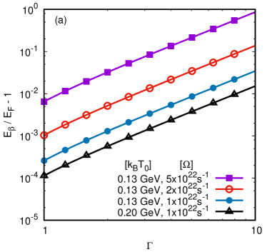
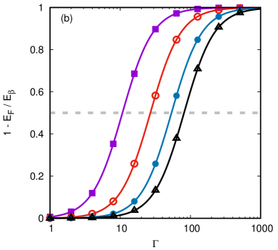
Figure 3: Relative differences (a) $E_{\beta}/E_{F}-1$ and (b) $1-E_{F}/E_{\beta}$ between the $\beta$-frame energy density $E_{\beta}$ (137) and the RKT result $E_{F}$ (27) for massless fermions. The curves correspond to $k_{\rm{B}}T_{0}=0.13\ {\rm GeV}$ (filled purple squares, empty red circles and filled blue circles) and $0.2\ {\rm GeV}$ (empty black triangles). The angular velocity is set to $\Omega=5\times 10^{22}\,{\rm s}^{-1}$ (filled purple squares), $2\times 10^{22}\,{\rm s}^{-1}$ (empty red circles) and $10^{22}\,{\rm s}^{-1}$ (filled blue circles and empty black triangles). The chemical potential on the rotation axis is $\mu_{0}=0.1\ {\rm GeV}$.

Figure 3(a) shows the relative departure of the QFT energy density $E_{\beta}$ (137) measured in the thermometer frame, compared to the RKT energy density $E_{F}=3P_{F}$ (27). We use values of the chemical potential and angular speed relevant for heavy ion collisions, as in section 2.2. For $k_{\rm{B}}T_{0}=0.2\ {\rm GeV}$ and $\Omega=10^{22}\,{\rm s}^{-1}$, the relative difference is about $10^{-4}$ on the rotation axis. From (138), this value can be increased by either increasing the angular velocity $\Omega$ or decreasing the temperature $T_{0}$. We thus also consider a lower temperature relevant to the QGP, $k_{\rm{B}}T_{0}\simeq 0.13\ {\rm GeV}$. This enlarges the relative difference by a factor of $\sim 2.4$. At larger values of the angular speed, quantum corrections are close to $1\%$ on the rotation axis. Away from the rotation axis, the relative difference $E_{\beta}/E_{F}-1$ increases roughly as $\Gamma^{2}$ (138). This is confirmed for all regimes considered in figure 3(a).

The relative difference $1-E_{F}/E_{\beta}$ is presented in figure 3(b). On the rotation axis, this ratio is negligible. As $\Gamma\rightarrow\infty$, equation (138) shows that the second term in the square bracket goes to $0$ and thus $\lim_{\Gamma\rightarrow\infty}1-E_{F}/E_{\beta}\rightarrow 1$. Close to the SLS, quantum corrections therefore become the dominant contribution to the energy density $E_{\beta}$. The gray, dashed line in figure 3(b) indicates where the quantum corrections become equal to the classical contribution, $E_{\beta}=2E_{F}$. This happens closer to the SLS when the temperature is increased or when the angular velocity is decreased.

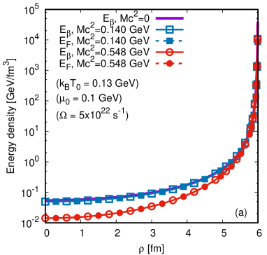
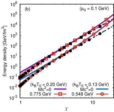
Figure 4: Dependence on (a) the distance $\rho$, measured in ${\rm fm}$ from the rotation axis, and (b) on the Lorentz factor $\Gamma$ (13), of the energy densities $E_{\beta}$ and $E_{F}$ obtained in QFT (empty symbols and continuous lines) and RKT (filled symbols and dashed lines) at $\mu_{0}=0.1\ {\rm GeV}$ and $\Omega=5\times 10^{22}\,{\rm s}^{-1}$. In (a), the temperature on the rotation axis is fixed at $k_{\rm{B}}T_{0}=0.13\ {\rm GeV}$ and the mass $Mc^{2}$ is set to $0$ (continuous purple line, only $E_{\beta}$ is shown), $0.140\ {\rm GeV}$ (blue squares) and $0.548\ {\rm GeV}$ (red circles). In (b), $k_{\rm{B}}T_{0}=0.20\ {\rm GeV}$ (upper lines) and $0.13\ {\rm GeV}$ (lower lines). The analytic results for the massless limit are shown using continuous (QFT) and dashed (RKT) lines without symbols (purple is used for $k_{\rm{B}}T_{0}=0.2\ {\rm GeV}$ and blue corresponds to $k_{\rm{B}}T_{0}=0.13\ {\rm GeV}$).

We next consider the effect of the mass on the energy density $E_{\beta}$. Figure 4(a) shows a comparison between the energy densities $E_{\beta}$ and $E_{F}$, as functions of the distance $\rho$ from the rotation axis. When $\Omega=5\times 10^{22}\,{\rm s}^{-1}$, the SLS is located at $\rho=c/\Omega=6\ {\rm fm}$. The energy density for particles of mass $0.14\ {\rm GeV}$ follows the result for the massless limit very closely, while the case with $Mc^{2}=0.548\ {\rm GeV}$ can be distinguished from the massless limit only up to $\rho\lesssim 5.5\ {\rm fm}$. Figure 4(b) shows the dependence of the energy densities $E_{\beta}$ and $E_{F}$ on the Lorentz factor $\Gamma$ (13). The RKT and QFT energy densities can be distinguished when $\Gamma\gtrsim 10$, where the higher order divergence induced by the quantum corrections becomes important. At large values of $\Gamma$, both the QFT and RKT energy densities follow their respective massless asymptotics, indicating that also in the QFT case, the corrections due to the mass terms contribute at a subleading order close to the SLS, compared with the corresponding massless limit.

Finally, we discuss the properties of quantum corrections on the rotation axis. Since the nonequilibrium terms vanish on the rotation axis, only the equilibrium quantities, $E_{\beta}$, $P_{\beta}$ and $Q_{\beta}$ need to be considered (we assume that $\varpi=0$ here). Instead of discussing $P_{\beta}$, we focus on the trace of the SET. Figure 5 shows the properties of the quantum corrections (a) $E_{\beta}/E_{F}-1$, (b) $(E_{\beta}-3P_{\beta})/(E_{F}-3P_{F})-1$ and (c) $Q_{\beta}/Q_{F}-1$, computed as relative differences between the QFT and RKT results.

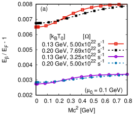
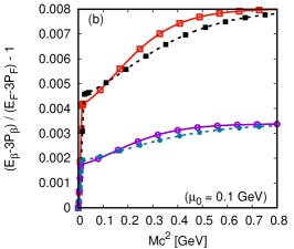
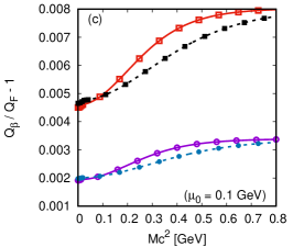
Figure 5: Relative differences (a) $E_{\beta}/E_{F}-1$, (b) $(E_{\beta}-3P_{\beta})/(E_{F}-3P_{F})-1$, (c) $Q_{\beta}/Q_{F}-1$, on the rotation axis ($\rho=0$), as functions of the particle mass. The chemical potential on the rotation axis is $\mu_{0}=0.1\ {\rm GeV}$, and the temperature on the rotation axis is set to $k_{\rm{B}}T_{0}=0.13\ {\rm GeV}$ (empty symbols and continuous lines) and $0.2\ {\rm GeV}$ (filled symbols and dashed lines). We consider angular speeds $\Omega$ equal to $5\times 10^{22}\,{\rm s}^{-1}$ (red empty squares with continuous lines and filled blue circles with dashed lines), $7.70\times 10^{22}\,{\rm s}^{-1}$ (black filled squares with dashed lines) and $3.25\times 10^{22}\,{\rm s}^{-1}$ (purple empty circles with continuous lines).

Focussing on the small mass regime, it can be seen that the relative quantum corrections of the SET trace exhibit a rapid variation with respect to $M$. This variation can be attributed to the presence of the sign function in the SET components (128), which can take negative values only when $Mc^{2}<\hbar\Omega/2$. In particular, the quantity $(E_{\beta}-3P_{\beta})/M^{2}c^{4}$ exhibits no quantum corrections with respect to the corresponding RKT quantity when $M=0$. A rapid increase can be seen at small masses bringing the relative quantum corrections to the SET trace from zero to the values observed for the other quantities (energy and charge density). At intermediate masses, a slow increase in the relative quantum corrections of all quantities can be seen. In the large mass limit, the relative quantum corrections seem to reach a plateau value.

8 Rigidly-rotating quantum systems in curved space-time

Thus far, we have focussed our attention on a quantum field in a rigidly-rotating state on unbounded Minkowski space-time. We have seen that thermal states for such a set-up cannot be defined if the quantum field is a scalar field Vilenkin:1980 ; Duffy:2002ss . However, it is possible to define rigidly-rotating thermal states for a quantum scalar field constrained within a cylindrical reflecting boundary enclosing the axis of rotation, providing the boundary lies completely within the SLS Vilenkin:1980 ; Duffy:2002ss . In this latter situation the rotating vacuum is identical to the nonrotating vacuum state and t.e.v.s are well-behaved. In Duffy:2002ss it is shown that the t.e.v.s in a corotating frame are very well approximated by the RKT quantities derived in section 2, except for a region close to the boundary, where the Casimir effect becomes important.

In this chapter we have shown that the situation on unbounded Minkowski space-time is very different for a fermion field compared to a scalar field Ambrus:2014uqa , in particular we can define a rotating fermion quantum vacuum state and rigidly-rotating thermal fermion states. T.e.v.s in these states are regular up to the SLS, where they diverge. A natural question is whether it is possible to consider a set-up similar to that for the scalar field, namely by including a reflecting boundary. For fermions, defining reflecting boundary conditions is more involved than it is for scalars (where one can simply impose, for example, Dirichlet boundary conditions). Using either nonlocal spectral boundary conditions Hortacsu:1980kv or the local MIT-bag boundary condition Chodos:1974je on a cylindrical boundary inside the SLS, the rotating fermion vacuum is identical to the nonrotating fermion vacuum Ambrus:2015lfr . Furthermore, rigidly-rotating thermal states have well-defined t.e.v.s, which are computed in Ambrus:2015lfr for the case of zero chemical potential. At sufficiently high temperatures, the t.e.v.s for the bounded scenario are very well approximated by the unbounded t.e.v.s we have discussed in sections 6 and 7, except for a region close to the boundary. In Chernodub:2017mvp it is shown that, as well as the “bulk” mode considered in Ambrus:2015lfr , the fermion field also has “edge states” localized near the boundary, which must also be taken into account. The effect of interactions for rigidly-rotating fermions inside a cylindrical boundary is studied in Chernodub:2016kxh ; Chernodub:2017ref .

In Minkowski space-time a rigidly-rotating quantum system is therefore unphysical unless an arbitrary boundary is introduced in such a way that there is no SLS. A natural question is whether rigidly-rotating quantum states exist in curved space-time. One advantage of working on Minkowski space-time is that, as well as having no curvature, the space-time has maximal symmetry, which simplifies many aspects of the analysis. To explore the effect of space-time curvature on rigidly-rotating quantum states, one may consider anti-de Sitter space-time (adS) Hawking:1973 ; Moschella2005 . This space-time has maximal symmetry but constant negative curvature. Furthermore, the boundary of the space-time is time-like, as is a cylindrical boundary in Minkowski space-time. In particular, appropriate conditions have to be applied to the field on the space-time boundary Avis:1977yn .

The properties of nonrotating thermal states on adS have been studied in the framework of RKT and QFT, for both scalars Ambrus:2018olh and fermions Ambrus:2018olh ; Ambrus:2017cow , in the absence of a chemical potential. The curvature of adS space-time affects these states in a number of ways. First, the normal-ordering procedure applied in section 5 is not valid in a general curved space-time due to the fact that v.e.v.s for the nonrotating vacuum are nonzero, for both scalars Kent:2014nya and fermions Ambrus:2015mfa . Unlike our Minkowski space-time results in section 5, the t.e.v.s for stationary states of both scalars and fermions receive quantum corrections in adS Ambrus:2018olh ; Ambrus:2017cow ; Ambrus:2017vlf .

What about rigidly-rotating quantum states in adS? Due to its time-like boundary, there is no SLS in adS if $\Omega{\mathcal{R}}<1$, where $\Omega$ is the angular speed and ${\mathcal{R}}$ is the radius of curvature of the space-time. In other words, if the radius of curvature is small and the angular speed not too large, there is no SLS. Rigidly-rotating quantum states on adS have been studied in much less detail than their Minkowski counterparts. For a quantum scalar field, it is known that the only possible choice of global vacuum state is the nonrotating vacuum Kent:2014wda , as in Minkowski space-time. One might conjecture that rigidly-rotating thermal states for scalars can be defined only if there is no SLS, but this question has yet to be addressed. For a quantum fermion field, the rotating and nonrotating vacua are identical if there is no SLS, while if an SLS is present, a distinct rotating vacuum state can be defined Ambrus:2014fka . The preliminary analysis in Ambrus:2014fka shows that rigidly-rotating thermal states have at least some features similar to those seen in sections 6 and 7 in Minkowski space-time, in particular the t.e.v.s diverge on the SLS (if there is one).

These results demonstrate that space-time curvature does have an effect on rigidly-rotating quantum states. Asymptotically-adS space-times in particular may be relevant for studying the QGP via gauge-gravity duality (see, for example, CasalderreySolana:2011us ; DeWolfe:2013cua ; Aharony:1999ti ; Ammon:2015wua for reviews). In this approach, string theory on an asymptotically adS space-time is dual to a conformal quantum field theory (CFT) on the boundary of adS (which itself is conformal to Minkowski space-time). The idea is that calculations on one side of the duality may shed light on phenomena on the other side. For example, thermal states in the boundary CFT would correspond to asymptotically adS black holes in the bulk. This is because black holes emit thermal quantum radiation Hawking:1974sw , the temperature of the radiation being known as the Hawking temperature. Asymptotically adS rotating black holes Carter:1968ks can be in thermal equilibrium with radiation at the Hawking temperature provided either the black hole rotation is not too large, or the adS radius of curvature is sufficiently small Hawking:1998kw . These conditions ensure that there is no SLS for these black holes. A full QFT computation of the t.e.v. of the stress-energy tensor for a quantum field on a rotating asymptotically adS black hole is, however, absent from the literature.

Some of the most astrophysically important space-times with rotation are Kerr black holes Kerr:1963ud . These black holes are asymptotically flat, that is, far from the black hole the space-time approaches Minkowski space-time, rather than adS space-time as for the black holes discussed in the previous paragraph. Kerr black holes therefore always have an SLS, a surface on which an observer must travel at the speed-of-light in order to corotate with the black hole’s event horizon. The quantum state describing a black hole in thermal equilibrium with radiation at the Hawking temperature is known as the Hartle-Hawking state Hartle:1976tp . In contrast to the situation for asymptotically adS rotating black holes, such a state cannot be defined for a quantum scalar field on an asymptotically flat Kerr black hole Kay:1988mu ; Ottewill:2000qh . Indeed, it can be shown that any quantum state which is isotropic in a frame rigidly-rotating with the event horizon of the black hole must be divergent at the SLS Ottewill:2000yr . If the black hole is enclosed inside a reflecting mirror sufficiently close to the event horizon of the black hole, then a Hartle-Hawking state can be defined for a quantum scalar field Duffy:2005mz . Interestingly, this state is not exactly rigidly-rotating with the angular speed of the horizon Duffy:2005mz . For a quantum fermion field, it is possible to define a Hartle-Hawking-like state on the Kerr black hole without the mirror present Casals:2013 . While this state is also not exactly rigidly-rotating, it is nonetheless divergent on the SLS Casals:2013 .

Rotating black hole space-times are much more complicated that the toy model of rigidly-rotating states on Minkowski space-time that we consider in this chapter. However, the key physics remains the same in both situations. Namely, rigidly-rotating states cannot be defined for a quantum scalar field if there is an SLS present. Rigidly-rotating thermal states can be defined for a quantum fermion field, even when there is an SLS, but such states diverge as the SLS is approached.

9 Summary

In this chapter we have considered the properties of rigidly-rotating systems in QFT. Our toy models are free massive scalar and fermion fields on unbounded flat space-time. Such systems cannot be realized in nature due to the presence of the SLS, the surface outside which particles must travel faster than the speed of light in order to be rigidly rotating. Nonetheless, this approach has revealed some interesting physics which is relevant to more realistic set-ups, such as the QGP as formed in heavy-ion collisions or quantum fields on black hole space-times.

We began the chapter by briefly reviewing the properties of rigidly-rotating thermal states for scalar and fermion particles within the framework of RKT. The main feature is that, for both scalars and fermions, macroscopic quantities such as the energy and pressure diverge on the SLS but are regular inside it.

Next we constructed rigidly-rotating thermal states within the canonical quantization approach to QFT on unbounded Minkowski space-time. Here there is a significant difference between scalar and fermion fields. In particular, rigidly-rotating thermal states for scalars cannot be defined. The quantization of the fermion field is less constrained than that of the scalar field, and as a result we are able to define rigidly-rotating thermal states for fermions. We computed the t.e.v.s of the FC, CC, AC and SET in these states. All t.e.v.s diverge on the SLS but are regular inside it. Relative to the RKT results, the quantum t.e.v.s diverge more rapidly as the SLS is approached. Quantum corrections therefore dominate close to the SLS. We stress that the advantage of the canonical quantization approach considered in this chapter is that it allows t.e.v.s to be expressed in integral form, which can then be used to obtain analytic (in the massless case) or numerical (in the massive case) results in a non-perturbative fashion, with arbitrary numerical precision, even in the regime where quantum corrections are dominant.

The toy model considered in this chapter is a good approximation to more physical rigidly-rotating systems enclosed inside a reflecting boundary, except in the vicinity of the boundary. The key physics features are also shared with more complicated systems in curved space-time. We therefore conclude that our method based on canonical quantization can serve as a reliable tool to compute t.e.v.s in rigidly-rotating systems of particles, in particular in set-ups relevant to relativistic heavy-ion collisions, from the nearly-classical regime to the quantum-dominated regime, with arbitrary numerical precision.

- (1) Meier, D.L.: Black hole astrophysics: the engine paradigm. Springer-Verlag, Berlin-Heidelberg, Germany (2012).
- (2) Chandrasekhar, S.: The mathematical theory of black holes. Oxford University Press, Oxford, United Kingdom (1985).
- (3) Hawking, S.W.: Particle creation by black holes. Commun. Math. Phys. 43, 199–220. (1975).
- (4) Frolov, V.P., Thorne, K.S.: Renormalized stress-energy tensor near the horizon of a slowly evolving, rotating black hole. Phys. Rev. D 39, 2125–2154 (1989).
- (5) Kay B.S., Wald, R.M.: Theorems on the uniqueness and thermal properties of stationary, nonsingular, quasifree states on space-times with a bifurcate Killing horizon. Phys. Rept. 207, 49–136 (1991).
- (6) Casals, M., Dolan, S.R., Nolan, B.C., Ottewill, A.C., Winstanley, E.: Quantization of fermions on Kerr space-time. Phys. Rev. D 87, 064027 (2013).
- (7) Jacak, B.V., Müller, B.: The exploration of hot nuclear matter. Nature 337, 310–314 (2012).
- (8) Kharzeev, D.E., Liao, J., Voloshin, S.A., Wang, G.: Chiral magnetic and vortical effects in high-energy nuclear collisions – a status report. Prog. Part. Nucl. Phys. 88, 1–28 (2016).
- (9) STAR Collaboration, Global -hyperon polarization in nuclear collisions. Nature 548, 62–65 (2017).
- (10) STAR Collaboration, Global polarization of -hyperons in Au+Au collisions at . Phys. Rev. C 98, 014910 (2018).
- (11) Florkowski, W., Friman, B., Jaiswal, A., Speranza, E.: Relativistic fluid dynamics with spin. Phys. Rev. C 97, 041901 (2018).
- (12) Becattini, F., Florkowski, W., Speranza, E.: Spin tensor and its role in non-equilibrium thermodynamics. Phys. Lett. B 789, 419–425 (2019).
- (13) Buzzegoli, M., Becattini, F.: General thermodynamic equilibrium with axial chemical potential for the free Dirac field. JHEP 12, 002 (2018).
- (14) Cercignani, C., Kremer, G.M.: The relativistic Boltzmann equation: theory and application. Birkhäuser Verlag, Basel, Switzerland (2002).
- (15) Becattini, F., Bucciantini, L., Grossi, E., Tinti, L.: Local thermodynamical equilibrium and the -frame for a quantum relativistic fluid. Eur. Phys. J. C 75, 191 (2015).
- (16) Becattini, F., Grossi, E.: Quantum corrections to the stress-energy tensor in thermodynamic equilibrium with acceleration. Phys. Rev. D 92, 045037 (2015).
- (17) Ambru\cbs, V. E. Helical massive fermions under rotation, JHEP 08, 016 (2020).
- (18) Ambru\cbs, V. E., Chernodub, M. N. Helical vortical effects, helical waves, and anomalies of Dirac fermions, arXiv:1912.11034 [hep-th].
- (19) Jaiswal, A., Friman, B., Redlich, K.: Relativistic second-order dissipative hydrodynamics at finite chemical potential. Phys. Lett. B 751, 548–552 (2015).
- (20) Wang, Q.: Global and local spin polarization in heavy ion collisions: a brief overview. Nucl. Phys. A 967, 225–232 (2017).
- (21) Huang, X.-G., Koide, T.: Shear viscosity, bulk viscosity, and relaxation times of causal dissipative relativistic fluid-dynamics at finite temperature and chemical potential. Nucl. Phys. A 889, 73–92 (2012).
- (22) Tanabashi, M. et al (Particle Data Group): The review of particle physics. Phys. Rev. D 98, 030001 (2018).
- (23) Ambru\cbs, V.E., Blaga, R.: Relativistic rotating Boltzmann gas using the tetrad formalism. Ann. West Univ. Timisoara, Ser. Phys. 58, 89–108 (2015).
- (24) Florkowski, W., Ryblewski, R., Strickland, M.: Testing viscous and anisotropic hydrodynamics in an exactly solvable case. Phys. Rev. C 88, 024903 (2013).
- (25) Kapusta, J.I., Landshoff, P.V.: Finite-temperature field theory. J. Phys. G: Nucl. Part. Phys. 15, 267–285 (1989).
- (26) Vilenkin, A.: Quantum field theory at finite temperature in a rotating system. Phys. Rev. D 21, 2260–2269 (1980).
- (27) Itzykson, C., Zuber, J.B.: Quantum field theory. Mcgraw-Hill, New York (1980).
- (28) Duffy, G., Ottewill, A.C.: The rotating quantum thermal distribution. Phys. Rev. D 67, 044002 (2003).
- (29) Ambru\cbs, V.E., Winstanley, E.: Rotating quantum states. Phys. Lett. B 734, 296–301 (2014).
- (30) Letaw, J.R., Pfautsch, J.D.: The quantized scalar field in rotating coordinates. Phys. Rev. D 22, 1345–1351 (1980).
- (31) Nicolaevici, N.: Null response of uniformly rotating Unruh detectors in bounded regions. Class. Quantum Grav. 18, 5407–5411 (2001).
- (32) Iyer, B.R.: Dirac field theory in rotating coordinates. Phys. Rev. D 26, 1900–1905 (1982).
- (33) Ambru\cbs, V.E., Winstanley, E.: Rotating fermions inside a cylindrical boundary. Phys. Rev. D 93, 104014 (2016).
- (34) Olver, F.W.J., Lozier, D.W., Boisvert, R.F., Clark, C.W.: NIST handbook of mathematical functions. Cambridge University Press, New York (2010).
- (35) Rezzolla, L., Zanotti, O.: Relativistic hydrodynamics. Oxford University Press, Oxford, United Kingdom (2013).
- (36) Prokhorov, G.Y., Teryaev, O.V., Zakharov, V.I.: Axial current in rotating and accelerating medium. Phys. Rev. D 98, 071901 (2018).
- (37) Vilenkin, A.: Macroscopic parity-violating effects: Neutrino fluxes from rotating black holes and in rotating thermal radiation. Phys. Rev. D 20, 1807–1812 (1979).
- (38) Prokhorov, G.Y., Teryaev, O.V., Zakharov, V.I.: Effects of rotation and acceleration in the axial current: density operator vs Wigner function. JHEP 02, 146 (2019).
- (39) Becattini, F., Chandra, V., Del Zanna, F., Grossi, E.: Relativistic distribution function for particles with spin at local thermodynamical equilibrium. Ann. Phys. 338, 32–49 (2013).
- (40) Ván, P., Biró, T.S.: First order and stable relativistic dissipative hydrodynamics. Phys. Lett. B 709, 106–110 (2012).
- (41) Ván, P., Biró, T.S.: Dissipation flow-frames: particle, energy, thermometer. In: Pilotelli, M., Beretta, G.P. (eds.): Proceedings of the 12th Joint European Thermodynamics Conference, Cartolibreria SNOOPY, 2013, pp. 546–551. arXiv:1305.3190 [gr-qc].
- (42) Bouras, I., Molnár, E., Niemi, H., Xu, Z., El, A., Fochler, O., Greiner, C., Rischke, D.H.: Investigation of shock waves in the relativistic Riemann problem: A comparison of viscous fluid dynamics to kinetic theory. Phys. Rev. C 82, 024910 (2010).
- (43) Duff, M.J.: Twenty years of the Weyl anomaly. Class. Quantum Grav. 11, 1387–1404 (1994).
- (44) Ambru\cbs, V.E.: Quantum non-equilibrium effects in rigidly-rotating thermal states. Phys. Lett. B 771, 151–156 (2017).
- (45) Hortacsu, M., Rothe, K.D., Schroer, B.: Zero energy eigenstates for the Dirac boundary problem. Nucl. Phys. B 171, 530–542 (1980).
- (46) Chodos, A., Jaffe, R.L., Johnson, K., Thorn, C.B., Weisskopf, V.F.: A new extended model of hadrons. Phys. Rev. D 9, 3471–3495 (1974).
- (47) Chernodub, M.N., Gongyo, S.: Edge states and thermodynamics of rotating relativistic fermions under magnetic field. Phys. Rev. D 96, 096014 (2017).
- (48) Chernodub, M.N., Gongyo, S.: Interacting fermions in rotation: chiral symmetry restoration, moment of inertia and thermodynamics. JHEP 1701, 136 (2017).
- (49) Chernodub, M.N., Gongyo, S.: Effects of rotation and boundaries on chiral symmetry breaking of relativistic fermions. Phys. Rev. D 95, 096006 (2017).
- (50) Hawking, S.W., Ellis, G.F.R.: The large-scale structure of space-time. Cambridge University Press, Cambridge, United Kingdom (1973).
- (51) Moschella, U.: The de Sitter and anti-de Sitter sightseeing tour. Séminaire Poincaré 1, 1–12 (2005).
- (52) Avis, S.J., Isham C.J., Storey, D.: Quantum field theory in anti-de Sitter space-time. Phys. Rev. D 18, 3565–3576 (1978).
- (53) Ambru\cbs, V.E., Kent, C., Winstanley, E.: Analysis of scalar and fermion quantum field theory on anti-de Sitter spacetime. Int. J. Mod. Phys. D 27, 1843014 (2018).
- (54) Ambru\cbs, V.E., Winstanley, E.: Thermal expectation values of fermions on anti-de Sitter space-time. Class. Quant. Grav. 34, 145010 (2017).
- (55) Kent C., Winstanley E.: Hadamard renormalized scalar field theory on anti-de Sitter spacetime. Phys. Rev. D 91, 044044 (2015).
- (56) Ambru\cbs V.E., Winstanley E.: Renormalised fermion vacuum expectation values on anti-de Sitter space-time. Phys. Lett. B 749, 597–602 (2015).
- (57) Ambru\cbs, V.E., Winstanley, E.: Quantum corrections in thermal states of fermions on anti-de Sitter space-time. AIP Conf. Proc. 1916, 020005 (2017).
- (58) Kent, C., Winstanley, E.: The global rotating scalar field vacuum on anti-de Sitter space-time. Phys. Lett. B 740, 188–191 (2015).
- (59) Ambru\cbs, V.E., Winstanley, E.: Dirac fermions on an anti-de Sitter background. AIP Conf. Proc. 1634, 40–49 (2015).
- (60) Casalderrey-Solana, J., Liu, H., Mateos, D., Rajagopal, K., Wiedemann, U.A.: Gauge/string duality, hot QCD and heavy ion collisions. Cambridge University Press, Cambridge, United Kingdom (2014).
- (61) DeWolfe, O., Gubser, S.S., Rosen, C., Teaney, D.: Heavy ions and string theory. Prog. Part. Nucl. Phys. 75, 86–132 (2014).
- (62) Aharony, O., Gubser, S.S., Maldacena, J.M., Ooguri, H., Oz, Y.: Large N field theories, string theory and gravity. Phys. Rept. 323, 183–386 (2000).
- (63) Ammon M., Erdmenger, J.: Gauge/gravity duality : Foundations and applications. Cambridge University Press, Cambridge, United Kingdom (2015).
- (64) Carter, B.: Hamilton-Jacobi and Schrodinger separable solutions of Einstein’s equations. Commun. Math. Phys. 10, 280–310 (1968).
- (65) Hawking, S.W., Hunter C.J., Taylor, M.: Rotation and the adS/CFT correspondence. Phys. Rev. D 59, 064005 (1999).
- (66) Kerr, R.P.: Gravitational field of a spinning mass as an example of algebraically special metrics. Phys. Rev. Lett. 11, 237–238 (1963).
- (67) Hartle, J.B., Hawking, S.W.: Path integral derivation of black hole radiance. Phys. Rev. D 13, 2188–2203 (1976).
- (68) Ottewill, A.C., Winstanley, E.: The renormalized stress tensor in Kerr space-time: general results. Phys. Rev. D 62, 084018 (2000).
- (69) Ottewill A.C., Winstanley, E.: Divergence of a quantum thermal state on Kerr space-time. Phys. Lett. A 273, 149–152 (2000).
- (70) Duffy G., Ottewill, A.C.: The renormalized stress tensor in Kerr space-time: Numerical results for the Hartle-Hawking vacuum. Phys. Rev. D 77, 024007 (2008).