Blended Convolution and Synthesis for Efficient Discrimination of 3D Shapes

Abstract

Existing models for shape analysis directly learn feature representations on 3D point clouds. We argue that 3D point clouds are highly redundant and hold irregular (permutation-invariant) structure, which makes it difficult to achieve inter-class discrimination efficiently. In this paper, we propose a two-pronged solution to this problem that is seamlessly integrated in a single blended convolution and synthesis layer. This fully differentiable layer performs two critical tasks in succession. In the first step, it projects the input 3D point clouds into a latent 3D space to synthesize a highly compact and inter-class discriminative point cloud representation. Since, 3D point clouds do not follow a Euclidean topology, standard 2/3D convolutional neural networks offer limited representation capability. Therefore, in the second step, we propose a novel 3D convolution operator functioning inside the unit ball to extract useful volumetric features. We derive formulae to achieve both translation and rotation of our novel convolution kernels. Finally, using the proposed techniques we present an extremely light-weight, end-to-end architecture that achieves compelling results on 3D shape recognition and retrieval.

1 Introduction

The human world is three-dimensional, therefore optimally understanding and interpreting 3D data is an important research problem. Although deep convolutional neural networks (CNNs) have been greatly successful in 2D representation learning, they still do not provide an adequate solution to unique challenges that 3D data presents. Specifically, there are two main issues pertinent to 3D data: (a) 3D point clouds and rasterized voxel based representations encode redundant information thereby making inter-class discrimination difficult, (b) 3D convolutions generally operate in Euclidean space, whereas real-world 3D data lie on a non-Euclidean manifold. The representations thus learned fail to encode the true geometric structure of input shapes. The availability of low-cost 3D sensors and their vast applications in autonomous cars, medical imaging and scene understanding demands a fresh look towards solving the above-mentioned challenges.

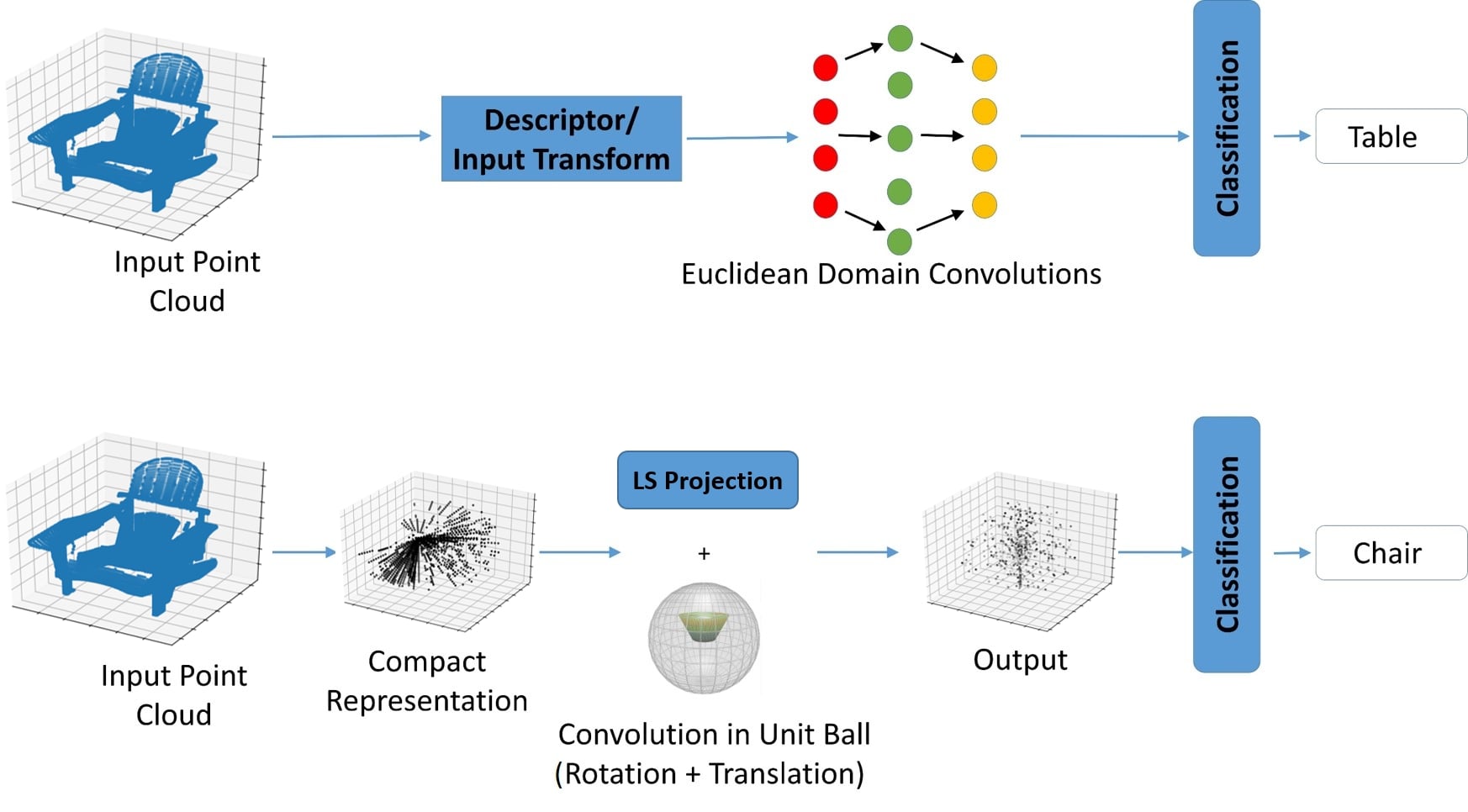
Figure 1: High-level comparison of our approach (bottom) with the traditional approaches [44, 53, 45, 32, 35] (top). We transform an input shape into a compact representation and project it onto a discriminative latent space to capture more discriminative features, before performing convolution in $\mathbb{B}^{3}$ with roto-translational kernels. Our novel convolution operator has a clear advantage over existing works that only work with Euclidean geometries. This results in a light-weight and highly efficient network design with significantly lower number of layers.

Existing representation learning schemes for 3D shape description either operate on voxels [7, 63] or point clouds [45, 32, 14, 15, 12, 13, 14]. The voxelized data representations are highly sparse, thus prohibiting the design of large-scale deep CNNs. Efficient data structures such as Octree [42] and Kdtree [6] have been proposed to solve this problem, however neural networks based representation learning on these tree-based indexing structures is an open research problem [49]. In comparison, point clouds offer an elegant, simple and compact representation for each point $(x,y,z)$. Additionally, they can be directly acquired from the 3D sensors, e.g., low-cost structured light cameras. On the down side, their irregular structure and high point redundancy pose a serious challenge for feature learning.

We note that recent attempts on direct feature learning from point clouds assume a simplistic pipeline (see Fig. 1) that mainly aims to extract better global features considering all points [44, 45, 32, 35]. However, all these approaches lack the capacity to work on non-Euclidean geometries and have no inherent mechanism to deal with the high redundancy of point clouds. In this work, we propose an integrated solution, called Blended Convolution and Synthesis (BCS), to address the above-mentioned problems. BCS can effectively deal with the irregular, permutation-invariant and redundant structure of point clouds. Our solution has two key aspects. First, we map the input 3D shape into a more discriminative 3D space. We posit that raw 3D point clouds are sub-optimal to be directly used as input to classification models, due to redundant information. This property hampers the classification and retrieval performance by adding an extra overhead to the network, as the network should then disregard redundant features purely using convolution. In contrast, we initially synthesize a more discriminative shape by projecting the original shape to a latent space using a newly derived set of functions which are complete in the unit ball ($\mathbb{B}^{3}$). The structure of this latent shape is governed by the loss function, and therefore, is optimized to pick up the most discriminative features. This step reduces the number of convolution layers significantly, as shown experimentally in Sec. 5. Second, we propose a new convolution operation that works on non-Euclidean typologies i.e., inside the unit ball ($\mathbb{B}^{3}$). We derive a novel set of complete functions within $\mathbb{B}^{3}$ that perform convolution in the spectral domain.

Furthermore, since our network operates on the ‘spectral domain’, it provides multiple advantages compared to competing models that operate in Euclidean domains: 1) A highly compact and structured representation of 3D objects, which addresses the problem of redundancy and irregularity. Effectively, a 3D shape is represented as a linear combination of complete-orthogonal functions, which allows only a few coefficients to encode shape information, compared to spatial domain representations. 2) Convolution is effectively reduced to a multiplication-like operator which improves computational efficiency, thereby significantly reducing the number of FLOPS. 3) A theoretically sound way to treat non-Euclidean geometries, which enables the convolution to achieve translational and rotational equivariance; and 4) Scalability to large-sized shapes with bounded complexity.

Most importantly, existing methods which perform convolution in the spectral domain [16, 18, 46] use spherical harmonics or Zernike polynomials to project 3D functions to the spectral domain for performing convolution. The aforementioned function spaces entail certain limitations, e.g.: 1) ‘Spherical harmonics’ only operate on the surface of the unit sphere, which causes critical information loss for non-polar shapes. 2) ‘Zernike polynomials’ cause the convolution to achieve only 3D rotational movement of the kernel. In contrast, our newly derived polynomials can handle non-polar shapes, while achieving both 3D rotational and translational movements of the convolution kernel as theoretically proved in Sec. 4.2. Recently, Jiang et al. [28] proposed a novel Fourier transform mechanism to optimally sample non-uniform data signals defined on different topologies to spectral domain without spatial sampling error. This allows CNNs to analyze signals on mixed topologies, regardless of the architecture. However, their spectral transformation does not specifically focus on computational efficiency and equivariance properties, as ours. On the other hand, Jingwei et al. [26] proposed a model which can directly segment textured 3D meshes, by extracting features from high-resolution signals on geodesic neighborhoods of surfaces. In contrast, our model consumes point clouds and we propose a lightweight convolution operator, which extracts useful features for 3D classification.

The main contributions of this work are:

• A novel approach to obtain a learned 3D shape descriptor, which enhances the convolutional feature extraction process, by projecting the input 3D shape into a latent space, using newly derived functions in $\mathbb{B}^{3}$.

• Develop the theory of a novel convolution operation, which allows both 3D rotational and 3D translational movements of the kernel.

• Derive formulae to perform discriminative latent space projection of the input shape and 3D convolution in a single step, thereby making our approach computationally efficient.

• Implement the proposed latent space projection and convolution as a fully differentiable module which can be integrated into any end-to-end learning architecture, and developing a shallow experimental network which produces results on par with state-of-the-art while being computationally efficient.

2 Related Work

3D shape descriptors: A 3D shape descriptor is a representation of the structural essence of a 3D shape. A variety of hand-crafted feature descriptors have been proposed in past research efforts. A few key such works are based on light field descriptors [11], Fourier transformation [59], eigen value descriptors [27], and geometric moments [17]. Most recent hand-crafted 3D descriptors are based on diffusion parameters [9, 50, 8]. On the other hand, learned 3D shape descriptors have also been popular in the computer vision literature. Litman et al. [39] propose a supervised bag-of-features (BOF) method to learn a descriptor. Zhu et al. follow an interesting approach, where they first project the 3D shapes into multiple 2D shapes, and then perform training on the 2D shapes to learn a descriptor. Xie et al. [67] present a hybrid approach which combines both hand-crafted features and deep networks. They first compute a geometric feature vector from the 3D shape, and then employ a deep network on the feature vector to learn a 3D descriptor. Xie et al. [66] follow a similar approach, where they first calculate heat kernel signatures of 3D shapes and then use two deep encoders to obtain descriptors. Our work is partially similar to this, but has a key difference: instead of computing hand-crafted features as the first step, we do a learned mapping of input 3D shape into a more discriminative 3D space, which allows us to get rid of high intra-class variances exhibited by most 3D shape descriptors. This step provides another advantage since it maximizes the distance between initial shapes, before being fed to convolution layers later.

Orthogonal Moments and 3D Convolution: Generally, orthogonal moments are used to obtain deformation invariant descriptors from structured data. Compared to geometric moments, orthogonal moments are robust to certain deformations such as rotation, translation and scaling. This property of orthogonal moments has been exploited specially in 2D data analysis in the past [25, 38, 1, 57, 30, 54]. Extension of deformation invariant moments from 2D to 3D also has been explored by many prior works [22, 48, 10, 19]. However, the certain properties of these moments depend on the Hilbert space on which they are defined. For example, orthogonal moments defined in a sphere or a ball exhibit convenient properties to extract rotation invariants, compared to orthogonal moments defined in a cube. These unique properties of orthogonal moments have recently been used to derive convolution operations which allows 3D rotational movements of kernels [16, 18, 46, 47]. However, the moments used in these works do not contain the necessary properties to achieve 3D translation of the kernels, and therefore, we derive a novel set of functions in $\mathbb{B}^{3}$ to overcome this limitation.

3D Shape Classification and Retrieval: Recent works developed for 3D shape classification and retrieval can be broadly categorized into three classes: 1) hand-crafted feature based [58], [23] 2) unsupervised learning based [63], [31] 3) deep learning based [44, 45, 37]. Generally, deep learning based approaches have shown superior results compared to other two categories. However, the aforementioned deep learning architectures operate on Euclidean spaces, which is sub-optimal for 3D shape analysis tasks, although Weiler et al. [62] has shown impressive results using SE(3)-equivariant convolutions in the Euclidean domain. In contrast, our network performs convolution on $\mathbb{B}^{3}$ which allows efficient feature extraction, since 3D rotation and translation of kernels are easier to achieve in this space.

3 Preliminaries

We first provide an overview of basic concepts that will be used later in proposed method.

3.1 Complete Orthogonal Systems

Orthogonal functions are useful tools in shape analysis. Let $\Phi_{m}$ and $\Phi_{n}$ be two functions defined in some space $\mathbb{S}$. Then, $\Phi_{m}$ and $\Phi_{n}$ are orthogonal over the space $\mathbb{S}$ if and only if,

$$\int_{\mathbb{S}}\Phi_{n}(X)\Phi_{m}(X)dX=0,\;\forall n\neq m.$$ (1)

Let $f$ be a function defined in space $\mathbb{S}$, and $\{\Phi_{m}\mathrel{\mathop{\ordinarycolon}}m\in\mathbb{Z}^{+}\}$ be a set of orthogonal functions defined in the same space. Then, the set of orthogonal moments of $f$, with respect to set $\{\Phi_{m}\}$, can be obtained by $\hat{f}_{m}=\int_{\mathbb{S}}f(X)\Phi_{m}(X)^{\dagger}$ where $\dagger$ denotes the complex conjugate. If a set of functions $\{\Phi_{m}\mathrel{\mathop{\ordinarycolon}}m\in\mathbb{Z}^{+}\}$ is both complete and orthogonal, it can reconstruct $f(X)$ using its orthogonal moments as follows,

$$f(X)=\sum_{m}\hat{f}_{m}\Phi_{m}(X).$$ (2)

3.2 Convolution in Unit Ball $\mathbb{B}^{3}$

The unit ball ($\mathbb{B}^{3}$) is the set of points $x\in\mathbb{R}^{3}$, where ${\parallel}x{\parallel}{<}1$. Any point in $\mathbb{B}^{3}$ can be parameterized using coordinates $(\theta,\phi,r)$, where $\theta,\phi$, and $r$ are azimuth angle, polar angle, and radius respectively. Performing convolution on 3D shapes in non-linear topological spaces such as the unit ball ($\mathbb{B}^{3}$) has a key advantage: compared to the Cartesian coordinate system, it is efficient to formulate 3D rotational movements of the convolutional kernel in $\mathbb{B}^{3}$ [46]. To this end, both the input 3D shape and the 3D kernel should be represented as functions in $\mathbb{B}^{3}$. However, performing convolution in the spatial domain is difficult due to non-linearity of $\mathbb{B}^{3}$ space [46]. Therefore, it is necessary to first obtain the spectral representation of the 3D shape and the 3D kernel, with respect to a set of orthogonal and complete functions in $\mathbb{B}^{3}$, and consequently perform spectral domain convolution.

4 Methodology

Here, we present our ‘Blended Convolution and Synthesis’ layer in detail. First, we construct a set of orthogonal and complete polynomials in $\mathbb{B}^{3}$. Then, we relax the orthogonality condition of these polynomials, which allows us to project the input shape to a latent space. This projection is a learned process and depends on the softmax cross-entropy between predicted and ground-truth object classes. Therefore, the projected shape is optimized to contain more discriminative properties across object classes. Afterwards, we convolve the latent space shape with roto-translational kernels in $\mathbb{B}^{3}$ to map it to the corresponding class. Besides, we derive formulae to achieve both projection and convolution in a single step, which makes our approach more efficient.

Below in Section 4.1, we explain the learned projection of the object onto a latent space. Then, in Section 4.2, we derive our convolution operation, which is able to capture features efficiently using roto-translational kernels.

4.1 Learned Mapping for Shape Synthesis

In this section, we explain the projection of 3D point clouds to a discriminative latent space in $\mathbb{B}^{3}$. First, we derive a set of complete orthogonal functions in $\mathbb{B}^{3}$. Orthogonal moments obtained using orthogonal functions can be used to reconstruct the original object. However, our requirement here is not to reconstruct the original object, but to map it to a more discriminative shape. Therefore, after deriving the orthogonal functions, we relax the orthogonality condition to facilitate the latent space projection. Furthermore, instead of the input point cloud, we use a compact representation as the input to the feature extraction layer, for efficiency and to leverage the capacity of convolution in $\mathbb{B}^{3}$. In Section 4.1.1, we explain our compact representation.

4.1.1 Compact Representation of Point Clouds

Most 3D object datasets contain point clouds with uniform texture. That is, if the 3D shape is formulated as a function $f$ in $\mathbb{B}^{3}$, such that for any point on the shape, $f(\theta,\phi,r)=c$, where $c$ is a constant. However, formulating 3D shapes in $\mathbb{B}^{3}$ has the added advantage of representing both 2D texture and 3D shape information simultaneously [46]. Therefore, the advantage of convolution in $\mathbb{B}^{3}$ can be utilized when the input and kernel functions have texture information.

Following this motivation, we convert the uniform textured point clouds into non-uniform textured point clouds using the following approach. First, we create a grid using equal intervals along $r,\theta$, and $\phi$. We use $25,36$, and $18$ interval spaces for $r,\theta$, and $\phi$, respectively. Then, we bin the point cloud to grid points, which results in a less dense, non-uniform surface valued point cloud. The obtained compact representation does not contain all the fine-details of the input point cloud. However in practice, it allows better feature extraction using the kernels. A possible reason could be that kernels are also non-uniform textured point clouds with discontinuous space representations, and they can capture better features from non-uniform textured input point clouds when performing convolution in $\mathbb{B}^{3}$.

4.1.2 Derivation of orthogonal functions in $\mathbb{B}^{3}$

In this section, we derive a novel set of orthogonal polynomials with necessary properties to achieve the translation and rotation of convolution kernels. Afterwards, in Section 4.1.4, we relax the orthogonality condition of the polynomials to facilitate latent space projection.

Canterakis et al. [10] showed that a set of orthogonal functions which are complete in unit ball can take the form $Z_{n,l,m}(r,\theta,\phi)=Q_{nl}(r)Y_{l,m}(\theta,\phi)$, where $Q_{nl}$ is the linear component and $Y_{l,m}(\theta,\phi)$ is the angular component. The variables $r$, $\theta$ and $\phi$ are radius, azimuth angle and polar angle, respectively. We choose $Y_{l,m}(\theta,\phi)$ to be spherical harmonics, since they are complete and orthogonal in $S^{2}$.

For the linear component, we do not use the Zernike linear polynomials as in Canterakis et al. [10], as they do not contain the necessary properties to achieve the translational behaviour of convolution kernels [46]. Therefore, we derive a novel set of orthogonal functions, which are complete in $0<r<1$, and can approximate any function in the same range. Furthermore, it is crucial that these functions contain necessary properties to achieve the translation of kernels while performing convolution. Therefore, we choose the following function as the base function:

$$f_{nl}=(-1)^{l}n\sum_{k=0}^{n}\frac{((n-l)r)^{k}}{k!}.$$ (3)

It can be seen that,

$$f_{nl}\approx(-1)^{l}n\exp(r(n-l)),$$ (4)

as $n$ increases, for small $r$. Therefore, we use the approximation given in Eq. 4 in future derivations. As we show in Section 4.2, this property is vital for achieving the translation of kernels. Next, we orthogonalize $f_{nl}(r)$ to obtain a new set of functions $Q_{nl}(r)$. Consider the orthogonality $\int_{\mathbb{B}^{3}}Z_{n,l,m}Z_{n^{\prime},l^{\prime},m^{\prime}}=0,\forall n\neq n^{\prime},l\neq l^{\prime},m\neq m^{\prime}$. If we consider only the linear component, the orthogonality condition should be $\int_{0}^{1}Q_{n,l}Q_{n^{\prime},l^{\prime}}r^{2}dr=0,\forall n\neq n^{\prime},l\neq l^{\prime}$. Therefore, $Q_{n,l}$ should be orthogonal with respect to the weight function $w(r)=r^{2}$. We define,

$$Q_{nl}(r)=f_{nl}(r)-\sum_{k=0}^{n-1}\sum_{m=0}^{k}C_{nlkm}Q_{km}(r)$$ (5)

where $n\geq 0,n\geq l\geq 0$ and $C_{nlkm}$ is a constant. Since $Q_{nl}$ should be an orthogonal set, the inner product between any two different $Q_{nl}$ functions is zero. Therefore, we obtain,

$$\langle Q_{nl},Q_{n^{\prime}l^{\prime}}\rangle =\langle f_{nl},Q_{n^{\prime}l^{\prime}}\rangle-\sum_{k=0}^{n-1}\sum_{m=0}^{k}C_{nlkm}\langle Q_{km},Q_{n^{\prime}l^{\prime}}\rangle$$

Since $\langle Q_{nl},Q_{n^{\prime}l^{\prime}}\rangle=0$, we get:

$$C_{nln^{\prime}l^{\prime}}=\frac{\langle f_{nl},Q_{n^{\prime}l^{\prime}}\rangle}{\parallel Q_{n^{\prime}l^{\prime}}\parallel^{2}}.$$ (6)

Following this process, we can obtain the set of orthogonal functions $Q_{nl}$ for $n\geq 0,n\geq l$. The derived polynomials up to $n=5,l=5$ are shown in Appendix A. In Section 4.1.3, we prove the completeness property of the derived functions.

4.1.3 Completeness in $\mathbb{B}^{3}$

In this section, we prove the completeness in $\mathbb{B}^{3}$ for the set of functions $\{Q_{nl}\}$ derived in Section 4.1.2.

Condition 1: Consider the orthogonal set $\{p_{n}\}$ defined in $L^{2}[0,1]$. Then, $\{p_{n}\}$ is complete in space $L^{2}[0,1]$ if and only if there is no non-zero element in $L^{2}[0,1]$ that is orthogonal to every $\{p_{n}\}$.

To show that $f_{nl}$ is complete over $L^{2}[0,1]$, we first prove the completeness of the set $\{\Phi_{n}\}$, which is obtained by orthogonalizing the set $\{1,x,x^{2},x^{3},...\}$. Let $\Psi(x)$ be an element in $L^{2}[0,1]$, which is orthogonal to every element of $\{1,x,x^{2},x^{3},...\}$. Then, suppose the following relationship is true:

$$\langle\Psi,e^{2\pi ikx}\rangle=\sum_{n=0}^{\infty}\frac{(2\pi ikn)^{n}}{n!}\langle\Psi,x^{n}\rangle=0,$$ (7)

where $k$ is a constant. However, we know that $\{e^{2\pi ikx}\}_{k=0}^{k=\infty}$ is the complex exponential Fourier basis, and is both complete and orthogonal. Therefore, if Eq. 7 is true, $\Psi=0$, which gives us the result, i.e., $\langle\Psi,x^{n}\rangle=0\equiv\,\Psi=0$. Equivalently, since $\{\Phi_{n}\}$ is obtained by orthogonalization of $\{1,x,x^{2},x^{3},...\}$, $\langle\Psi,\{\Phi_{n}\}\rangle=0\equiv\,\Psi$ = 0. Hence, according to Condition 1, $\{\Phi_{n}\}$ is complete in $L^{2}[0,1]$.

Next, we consider the set $Q_{n,l}$. Since $Q_{n,l}$ is orthogonalized using the basis functions in Eq. 18, it is enough to show that $f_{nl}$ is complete over $L^{2}[0,1]$. Let $\Theta$ be a function defined in $L^{2}[0,1]$. Then, suppose the following relationship is true:

$$\langle\Theta,f_{n,l}\rangle=(-1)^{l}n\sum_{k=0}^{n}\frac{((n-l)^{k}}{k!}\langle\Theta,r^{k}\rangle=0.$$ (8)

For Eq. 8 to be true, $\langle\Theta,r^{k}\rangle=0$ for $k=\{0,1,2,...\}$. But we showed that this condition is satisfied if and only if $\Theta=0$. Therefore, $\langle\Theta,f_{n,l}\rangle=0,\forall n\geq l\geq 0\equiv\,\Theta=0$. Hence, $f_{n,l}$ is complete in $L^{2}[0,1]$.

4.1.4 Relaxation of orthogonality of functions in $\mathbb{B}^{3}$

Computing $C_{nln^{\prime}l^{\prime}}$ using Eq. 6 ensures the orthogonality of $Q_{nl}$. Since $Q_{nl}$ and $Y_{lm}$ are both orthogonal and complete, projecting the input shape $f$ onto the set of functions $Z_{nlm},n\geq l\geq m\geq 0$, enables us to reconstruct $f$ by:

$$f(\theta,\phi,r)=\sum\limits_{n=0}^{\infty}\sum\limits_{l=0}^{n}\sum\limits_{m=-l}^{l}\Omega_{n,l,m}(f)Z_{n,l,m}(\theta,\phi,r),$$ (9)

where spectral moment $\Omega_{n,l,m}(f)$ can be obtained using $\Omega_{n,l,m}(f)=\int_{0}^{1}\int_{0}^{2\pi}\int_{0}^{\pi}f(\theta,\phi,r){Z}_{n,l,m}r^{2}\sin\phi\,drd\phi d\theta.$. Representing $f$ in spectral terms, as in Eq. 9, enables easier convolution in spectral space, as derived in Section 4.2.

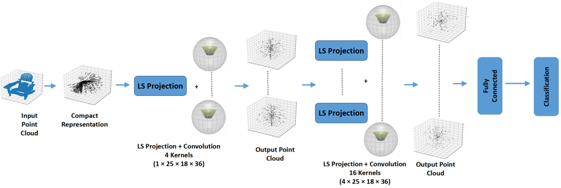
Figure 2: The overall CNN architecture. Our proposed design is a light-weight model, comprising of only three weight layers. Our networks aims to achieve a compact latent representation and volumetric feature learning via convolutions in $\mathbb{B}^{3}$.

However, we argue that since 3D point clouds across different object classes contain redundant information, projecting the point clouds in to a more discriminative latent space can improve classification accuracy. Our aim here is to reduce redundant information and noise from the input point clouds and map it to a more discriminative point cloud, which concentrates on discriminative geometric features. Therefore, we make $C_{nln^{\prime}l^{\prime}}$ trainable, which allows the latent space projection $\hat{f}$ of the input shape $f$ as follows:

$$\hat{f}(\theta,\phi,r)=\sum\limits_{n=0}^{\infty}\sum\limits_{l=0}^{n}\sum\limits_{m=-l}^{l}\hat{\Omega}_{n,l,m}(f)\hat{Z}_{n,l,m}(\theta,\phi,r),$$ (10)

where spectral moment $\hat{\Omega}_{n,l,m}(f)$ can be obtained using,

$$\hat{\Omega}_{n,l,m}(f)=\int_{0}^{1}\int_{0}^{2\pi}\int_{0}^{\pi}f(\theta,\phi,r){\hat{Z}}^{\dagger}_{n,l,m}r^{2}\sin\phi\,drd\phi d\theta,$$

where $\hat{Z}_{n,l,m}(\theta,\phi,r)=\hat{Q}_{nl}(r)Y_{lm}(\theta,\phi)$ and $\hat{Q}_{nl}(r)=f_{nl}(r)-\sum_{k=0}^{n-1}\sum_{m=0}^{k}W_{nlkm}\hat{Q}_{km}(r)$. Here, the set $\{W_{nlkm}\}$ denotes trainable weights. Note that since the final orthogonal function is a product of the linear and the angular parts, making both functions learnable is redundant.

4.2 Convolution of functions in $\mathbb{B}^{3}$

Let the north pole be the $y$ axis of the Cartesian coordinate system and the kernel is symmetric around $y$. Let $f(\theta,\phi,r)$, $g(\theta,\phi,r)$ be the functions of object and kernel respectively. Then, convolution of functions in $\mathbb{B}^{3}$ is defined by:

$$f*g(\alpha,\beta,r^{\prime})\coloneqq\langle f(\theta,\phi,r),T_{r}^{\prime}\{\tau_{(\alpha,\beta)}(g(\theta,\phi,r))\}\rangle$$ (11)

$${=}{\int_{0}^{1}}{\int_{0}^{2\pi}}{\int_{0}^{\pi}}f(\theta,\phi,r)T_{r}^{\prime}\{\tau_{(\alpha,\beta)}(g(\theta,\phi,r))\}\sin\phi\,d\phi d\theta dr,$$

where $\tau_{(\alpha,\beta)}$ is an arbitrary rotation that aligns the north pole with the axis towards the $(\alpha,\beta)$ direction ($\alpha$ and $\beta$ are azimuth and polar angles respectively) and $T_{r}^{\prime}$ is translation by $r^{\prime}$.

To achieve both latent space projection and convolution in $\mathbb{B}^{3}$ in single step, we present the following theorem.

Theorem 1: Suppose $f,g\mathrel{\mathop{\ordinarycolon}}X\longrightarrow\mathbb{R}^{3}$ are square integrable functions defined in $\mathbb{B}^{3}$ so that $\langle f,f\rangle<\infty$ and $\langle g,g\rangle<\infty$. Further, suppose $g$ is symmetric around the north pole and $\tau(\alpha,\beta)=R_{y}(\alpha)R_{z}(\beta)$ where $R\in\mathbb{SO}(3)$ and $T_{r}^{\prime}$ is translation of each point by $r^{\prime}$. Then,

$$\int_{0}^{1}\int_{0}^{2\pi}\int_{0}^{\pi}P\{f(\theta,\phi,r)\}T_{r}^{\prime}\{\tau_{(\alpha,\beta)}(g(\theta,\phi,r))\}\sin\phi\,d\phi d\theta dr$$

$$\approx\frac{4\pi}{3}\sum\limits_{n=0}^{\infty}\sum\limits_{l=0}^{n}\sum\limits_{m=-l}^{l}\langle f_{nl}(r),Q_{n^{\prime}l}(r)\rangle(e^{(n-l)r^{\prime}}-e^{(n^{\prime}-l)r^{\prime}})$$

$$\qquad\hat{\Omega}_{n,l,m}(f)\hat{\Omega}_{n,l,0}(g)Y_{l,m}(\theta,\phi),$$ (12)

where, $\hat{\Omega}_{n,l,m}(f),\hat{\Omega}_{n,l,0}(g)$ and $Y_{l,m}(\theta,\phi)$ are $(n,l,m)^{th}$ spectral moment of $f$, $(n,l,0)^{th}$ spectral moment of $g$, and spherical harmonics function, respectively. $P\{\cdot\}$ is the projection to a latent space, $\tau(\alpha,\beta)=R_{y}(\alpha)R_{z}(\beta)$ where $R\in\mathbb{SO}(3)$ and $T_{r}$ is translation of each point by $r$. The proof to this theorem can be found in Appendix A.

4.3 Network Architecture

Our experimental architecture consists of two convolution layers and a fully connected layer. We employ four kernels in the first convolution layer and 16 kernels in the second convolution layer, each followed by group normalization [64] and a ReLU layer. The experimental architecture is illustrated in Figure 2. We use $n=5$ for implementing Eq. 11 and softmax cross-entropy loss as the objective function during training. For training, we use a two step process. First, we train polynomial weights using a learning rate of $10^{-5}$, and then train kernel weights using a learning rate of $0.01$. We used the Adam optimizer for calculating gradients with parameters $\beta_{1}=0.9$, $\beta_{2}=0.999$, and $\epsilon=1\times 10^{-8}$, where parameters refer to the usual notation. We use $20k$ iterations to train polynomials weights and $30k$ iterations to train kernel weights. We use a single GTX 1080Ti GPU for training and the model takes around 30 minutes to complete a single epoch during training on ModelNet10 dataset.

Method	Modality	Views	#Layers	ModelNet10	ModelNet40
VoxNet (IROS’15) [41]	Volume	-	-	92.0%	83.0%
3DGAN (NIPS’16) [63]	Volume	-	-	91.0%	83.3%
3DShapeNet (CVPR’15) [65]	Volume		4-3DConv + 2FC	83.5%	77%
VRN ((NIPS’16)) [7]	Volume	-	45Conv	93.6%	91.3 %
GIFT ((CVPR’16)) [3]	RGB	64	-	92.4%	83.1%
Pairwise ((CVPR’16)) [29]	RGB	12	23Conv	92.8%	90.7%
MVCNN (ICCV’16) [53]	RGB	12	60Conv + 36FC	-	90.1%
MHBN (CVPR’18) [68]	RGB	6	78Conv + 18FC	95.0%	94.7%
DeepPano (SPL’15) [51]	RGB		4Conv + 3FC	85.5%	77.63%
ECC (CVPR’17) [52]	Points	-	4Conv + 1FC	90.0%	83.2%
Kd-Networks (ICCV’17) [32]	Points	-	15KD	93.5%	91.8%
SO-Net (CVPR’18) [35]	Points		11FC	95.7%	93.4%
PointNet (CVPR’17) [44]	Points	-	5Conv + 2STL	-	89.2%
LP-3DCNN (CVPR’19) [33]	Points	-	15Conv + 3FC	-	92.1%
Ours	Points	-	2Conv + 1FC	94.2%	91.8%

Table 1: Model accuracy vs depth analysis on ModelNet10 and ModelNet40 datasets.

Method	FLOPS	ModelNet40
	(inference)
PointNet [44]	14.70B	89.2%
SpecGCN [60]	17.79B	92.1%
PCNN [2]	4.70B	92.3%
PointNet++ [45]	26.04B	91.9%
3DmFV-Net [5]	16.89B	91.6%
PointCNN [36]	25.30B	92.2%
DGCNN [61]	44.27B	93.5%
Ours	1.31B	91.8%

Table 2: Our model complexity is much lower compared to state-of-the-art 3D classification models. The FLOPS (inference time) comparisons are reported according to [36] settings with 16 batch size.

5 Experiments

We evaluate the proposed methodology on 3D object classification and 3D object retrieval tasks using recent datasets: ModelNet10, ModelNet40, McGill 3D, SHREC’17 and OASIS. We also conduct a thorough ablation study to demonstrate the effectiveness of our derivations and design choices.

5.1 3D Object Classification Performance

A key feature of our proposed pipeline is the projection of the input 3D shapes into a more discriminative latent shape, before feeding them into convolution layers. One critical advantage of this step is that original subtle differences across object classes are magnified in order to leverage the feature extraction capacity of convolution layers. Therefore, the proposed network should be able to capture more discriminative features in the lower layers, and provide better classification results with a smaller number of layers, compared to other state-of-the-art works which directly extract features from the original shape. To illustrate this, we present a model depth vs accuracy analysis on ModelNet10 and ModelNet40 in Table 1, and compare the effectiveness of our network with other comparable state-of-the-art approaches.

State-of-the-art work can be mainly categorized into three types: volume based, RGB based and Points based. Volume based methods generally rely on volumetric representation of the 3D shape such as voxels. VoxNet [41] shows the best performance among volume based models, with an accuracy of 92.0% in ModelNet10 and 83.0% in ModelNet40, which is lower than our model’s accuracy. It is interesting to see that 3DShapeNets [65], and VRN [7] have significantly more layers compared to our model, although accuracies are lower. In general, our model performs better and has a lower model depth compared to volume based methods.

RGB based models generally follow the projection of the 3D shape into 2D representations, as an initial step for feature extraction. We perform better than all the RGB based methods, except for MHBN [68], which has accuracies 95.0% and 94.7% over ModelNet10 and ModelNet40 respectively. However, MHBN contains six views and for each view they employ a VGG-M network for initial feature extraction. This results in a significantly complex setup, which contains 96 trainable layers. In contrast, our model uses a single view and three trainable layers. Generally, RGB based models use multiple views, pre-trained deep networks and ensembled models, which results in increased model complexity. In contrast, our model use a single view and does not use pre-trained models, and achieves the second highest performance compared to RGB based models.

Point based models directly consume point clouds. Our model achieves the second best performance in this category, the highest being SO-NET [35]. However, SO-NET contains 11 fully connected layers, while our model only contains three layers. Our model is able to outperform the other point based setups, although their model depths are larger.

Overall, our model achieves a performance mark comparable to the best models, with a much shallower architecture. Our model contains the lowest number of trainable layers compared to all the models. This analysis on ModelNet10 and ModelNet40 clearly reveals the efficiency and better feature extraction capacity of our approach. Table 2 depicts the computational efficiency of BCS compared to state-of-the-art. With just $1.31$B FLOPs, we outperform the closest contender PCNN [2] by a significant $3.39$B margin.

5.2 3D Object Retrieval Performance

In this section, we compare the performance of our approach in 3D object retrieval. We use the McGill 3D dataset and SHREC’17 dataset for our experiments. We first obtain the feature vectors computed by each kernel in the second layer, and concatenate them. Then, we apply an autoencoder on the concatenated vector and retrieve a 1000-dimensional descriptor. Then we measure the cosine similarity between input and target shapes to measure the 3D object retrieval performance. We use the nearest neighbour performance and the evaluation metric. Table 3 depicts the results on the McGill Dataset. Out of the six state-of-the-art models compared, our model achieves the best retrieval performance. Table 4 illustrates the performance comparison on the SHREC’17 dataset, where our approach gives the second best performance, below Furuya et al. [21]. Figure 4 depicts our training curves for polynomial weights and kernel weights. The training curves are obtained for ModelNet10.

5.3 Ablation Study

In this section, we conduct an ablation study on our model and discuss various design choices, as illustrated in Figure 3. Firstly, we use a single convolution layer instead of two, and achieve an accuracy of 74.2% over ModelNet10. Then, we investigate the effect of using a higher number of convolution layers. We get accuracies 91.3% and 87.5%, when using three and four convolution layers respectively. Therefore, using two convolution layers yields the best performance. An important feature of our convolution layer is the translation of convolution kernels, in addition to rotation. To evaluate the effect of this, we use only rotating kernels and measure the performance, and achieve an accuracy of 80.2%. Therefore, it can be concluded that having the translational movements of the kernel has caused an accuracy increment of 14%, which is significant. Next, we measure the effect of latent space projection. To this end, we use orthogonal polynomials derived in Equations 5-6 for convolution, instead of making them learnable. This removes the latent space projection of the input, as the original object is reconstructed using spectral moments. After removing the latent space projection, the accuracy is dropped by 20.3%, which clearly reveals the significance of this feature. Then, we replace our convolution layers with volumetric convolution [46] layers and spherical convolution layers [16] and get 88.5% and 77.3% accuracy respectively. This shows that our convolution layer has a better feature extraction capacity compared to other convolution operations. One key reason behind this can be the translational movements of our kernels and the combined latent space projection step, which the aforementioned convolution methods lack.

Moreover, we test our model using basis functions in Eq. 18 as the projection functions, instead of learnable functions. Also, we again test the model using orthogonal functions. In both cases, the performance is lower compared to learnable functions. Furthermore, instead of soft-max cross entropy, we use WSoftmax [40] and GASoftmax [40] and achieve only 84.0% and 83.0% respectively. Therefore, using soft-max cross entropy as the loss function is justified. We also evaluate the effect of sampling density on accuracy. As shown in Figure 3, accuracy drops below 94.2%—which is reported by final architecture—when using a denser representation. Similarly, accuracy drops to 86.7% when using $r=10,\theta=18,\phi=9$ as sampling intervals. Therefore, using $r=25,\theta=36,\phi=18$ as in the final architecture seems to be the ideal design choice. We use four different distance measures in the 3D object retrieval task and compare the performance: cosine similarity, Euclidean distance, KL divergence, and Bhattacharya distance. Out of these, cosine similarity yields the best performance, with a mAP of 0.466.

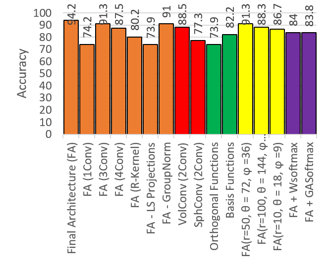
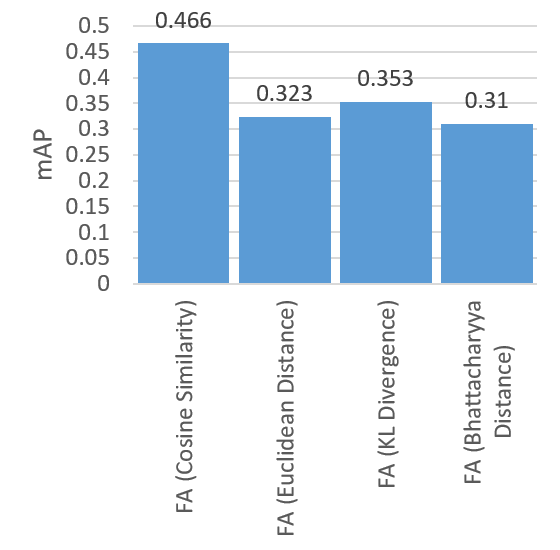
Figure 3: Ablation study on ModelNet10 in 3D object classification (left) and SHREC’17 in 3D object retrieval (right).

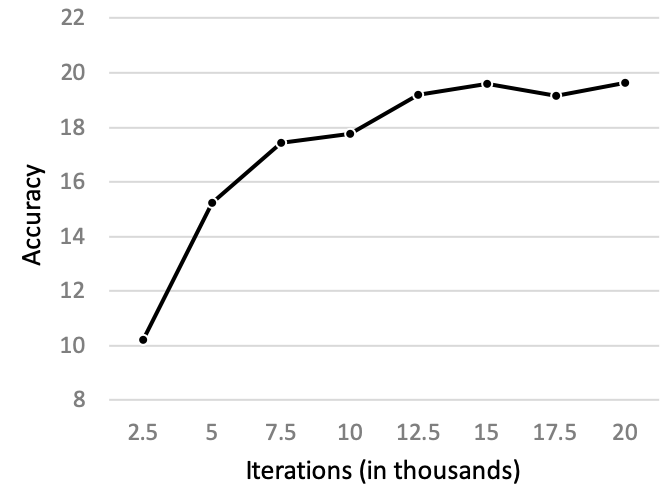
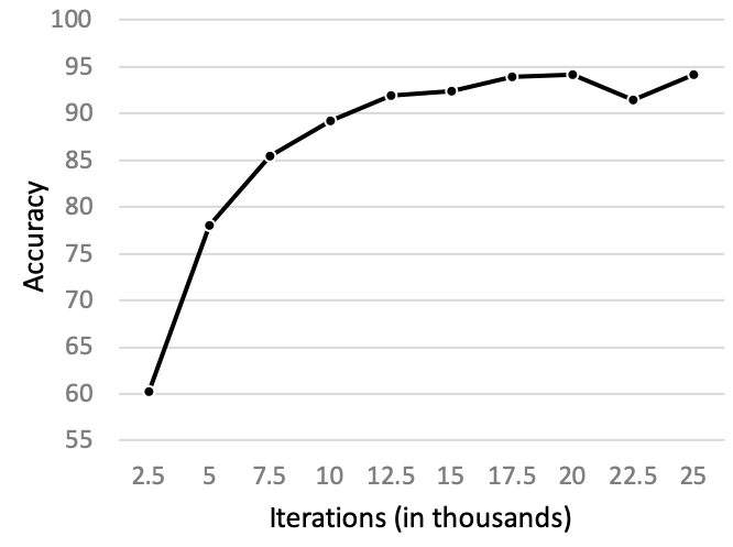
Figure 4: Training curves of our architecture on ModelNet10 for polynomial weights (left) and kernel weights (right).

Table 3: 3D object retrieval results comparison with state-of-the-art on McGill Dataset.

Method	Accuracy
Bashiri et al. [4] (arxiv’19)	0.9646%
Zeng et al. [69] (IET’18)	0.981%
Han et al. [24] (IP’18)	0.8827%
Tabia et al. [55] (CVPR’14)	0.977%
Papadakis et al. [43] (3DOR’w)	0.957%
Lavoue et al. [34] (TVC’14)	0.925%
Xie et al. [66] (CVPR’15)	0.988%
Ours	0.990%

Table 4: 3D object retrieval results comparison with state-of-the-art on SHREC’17.

Method	mAP
Furuya et al. [21] (BMVC’16)	0.476
Esteves et al. [18] (ECCV’18)	0.444
Tatsuma et al. [56] (TVC’09)	0.418
Bai et al. [3] (CVPR’16)	0.406
Ours	0.466

5.4 Classification of Complex Shapes

The proposed convolution layer offers two key advantages: 1) the ability to simultaneously model both shape and texture information, and 2) handling non-polar objects. However, we used ModelNet10 to conduct the ablation study shown in Figure 4, which contains relatively simple shapes (i.e. not dense in $\mathbb{B}^{3}$), and it is clear from the results that the accuracy drops when more than two convolution layers are used. A possible reason for this behaviour is overfitting. Since our convolution layer can capture highly discriminative features from the input functions, using more parameters can cause overfitting on relatively simpler shapes, and thus, a drop in classification accuracy. To test this hypothesis, we conduct an experiment on a more challenging dataset, which contains highly non-polar and textured objects.

In this experiment, we use OASIS-3 dataset [20] to sample $1000$ 3D brain scan images. The dataset includes brain scan images from both Alzheimer’s disease patients and healthy subjects. A key property of these images is that they have texture information and are highly dense in $\mathbb{B}^{3}$. Firstly, we split the sampled data in to train and test sets, with $800$ and $200$ images for each set, respectively. To avoid bias, we include an equal number of Alzheimer cases and healthy cases in both train and test sets. Then, we evaluate different network architectures using the dataset, varying the number of convolution layers. We use cross entropy loss function in this experiment. The results are shown in Table 5.

Table 5: Multi-layer architectures for highly non-polar and textured shape classification. Our model shows an improvement with more layers.

Model	Accuracy
Ours (1 Conv layer)	66.3%
Ours (2 Conv layers)	82.7%
Ours (3 Conv layers)	86.7%
Ours (4 Conv layers)	88.1%
Ours (5 Conv layers)	87.0%

As evident from Table 5, the classification accuracy increases with the number of convolution layers, up to four layers. Hence, it can be concluded that more challenging objects allow our model to demonstrate its full capacity.

6 Conclusion

In this paper, we propose a novel approach called ‘Blended Convolution and Synthesis’ to analyse 3D data, which entails two key operations: (1) learning a 3D descriptor obtained by projecting the input 3D shape into a discriminative latent space and (2) convolving the 3D descriptor in $\mathbb{B}^{3}$ with roto-translational 3D kernels for extracting features. We derive a novel set of polynomials in $\mathbb{B}^{3}$, and project the input data into a spectral space using the derived polynomials to join these two operations into a single step. Furthermore, we use a compact representation of the input data to reduce the density of the data distribution and leverage the advantage of convolving functions in $\mathbb{B}^{3}$. Finally, we present a light-weight architecture and achieve compelling results in 3D object classification and 3D object retrieval tasks.

Appendix A
Blended Convolution and Synthesis for Efficient Discrimination of 3D Shapes

Appendix A The derived $Q_{nl}$ polynomials up to $n{=}5$, $m{=}5$:

$Q_{nl}$ polynomials up to $n=5$ and $m=5$ are shown in Table 6.

Table 6: The derived $Q_{nl}$ polynomials up to $n=5$, $m=5$.

Polynomial	Expression
$Q_{00}$	$0$
$Q_{10}$	$1.+2x$
$Q_{11}$	$-1.-1x$
$Q_{20}$	$-9.79-10.65x+9x^{2}$
$Q_{21}$	$5.29+6.29x-4x^{2}$
$Q_{22}$	$-1.99-3.63x+x^{2}$
$Q_{30}$	$-123.58-158.11x+87.46x^{2}+32x^{3}$
$Q_{31}$	$70.26+89.41x-50.31x^{2}-13.5x^{3}$
$Q_{32}$	$15.86+22.27x-11.06x^{2}-0.5x^{3}$
$Q_{33}$	$-768.81-1006.25x+512.65x^{2}+139.10x^{3}+104.16x^{4}$
$Q_{40}$	$-35.86-46.15x+25.59x^{2}+4x^{3}$
$Q_{41}$	$422.87+550.70x-287.81x^{2}-73.52x^{3}-42.66x^{4}$
$Q_{42}$	$-768.81-1014.25x+480.65x^{2}+73.77x^{3}+13.5x^{4}$
$Q_{43}$	$-776.81-1034.25x+454.65x^{2}+50.43x^{3}-2.66x^{4}$
$Q_{44}$	$-768.81-1022.25x+464.65x^{2}+56.43x^{3}+0.16x^{4}$
$Q_{50}$	$-3683.18-4855.97x+2342.20x^{2}+509.59x^{3}+340.36x^{4}+324x^{5}$
$Q_{51}$	$1960.80+2578.79x-1263.64x^{2}-280.02x^{3}-167.77x^{4}-130.20x^{5}$
$Q_{52}$	$-981.80-1286.88x+643.53x^{2}+141.74x^{3}+72.23x^{4}+42.66x^{5}$
$Q_{53}$	$463.12+604.69x-309.13x^{2}-64.52x^{3}-25.87x^{4}-10.12x^{5}$
$Q_{54}$	$-208.26-272.17x+140.81x^{2}+25.87x^{3}+7.44x^{4}+1.33x^{5}$
$Q_{55}$	$91.29+122.33x-61.70x^{2}-9.53x^{3}-2.07x^{4}-0.04x^{5}$

Appendix B Combined latent space projection and Volumetric Convolution with Roto-Translataional Kernels

Theorem 1: Suppose $f,g\mathrel{\mathop{\ordinarycolon}}X\longrightarrow\mathbb{R}^{3}$ are square integrable complex functions defined in $\mathbb{B}^{3}$ so that $\langle f,f\rangle<\infty$ and $\langle g,g\rangle<\infty$. Further, suppose $g$ is symmetric around north pole and $\tau(\alpha,\beta)=R_{y}(\alpha)R_{z}(\beta)$ where $R\in\mathbb{SO}(3)$ and $T_{r^{\prime}}$ is translation of each point by $r^{\prime}$. Then,

$$\begin{split}f*g(r^{\prime},\alpha,\beta)&\coloneqq\int_{0}^{1}\int_{0}^{2\pi}\int_{0}^{\pi}P\{f(\theta,\phi,r)\},T_{r^{\prime}}\{\tau_{(\alpha,\beta)}(g(\theta,\phi,r))\}\sin\phi\,d\phi d\theta dr\\ &\approx\frac{4\pi}{3}\sum\limits_{n=0}^{\infty}\sum\limits_{n^{\prime}=0}^{\infty}\sum\limits_{l=0}^{n}\sum\limits_{m=-l}^{l}\langle f_{nl}(r),Q_{n^{\prime}l}(r)\rangle(e^{(n-l)r^{\prime}}-e^{(n^{\prime}-l)r^{\prime}})\hat{\Omega}_{n,l,m}(f)\hat{\Omega}_{n^{\prime},l,0}(g)Y_{l,m}(\alpha,\beta),\end{split}$$ (13)

where $\hat{\Omega}_{n,l,m}(f),\hat{\Omega}_{n^{\prime},l,0}(g)$ and $Y_{l,m}(\theta,\phi)$ are $(n,l,m)^{th}$ spectral moment of $f$, $(n^{\prime},l,0)^{th}$ spectral moment of $g$, and spherical harmonics function respectively. $P\{\cdot\}$ is the projection to a latent space, $\tau(\alpha,\beta)=R_{y}(\alpha)R_{z}(\beta)$ where $R\in\mathbb{SO}(3)$ and $T_{r^{\prime}}$ is translation of each point by $r^{\prime}$.

Proof: The input function $f$ is projected to the latent space shape $\hat{f}$ by,

$$\hat{f}(\theta,\phi,r)=\sum\limits_{n=0}^{\infty}\sum\limits_{l=0}^{n}\sum\limits_{m=-l}^{l}\hat{\Omega}_{n,l,m}(f)\hat{Z}_{n,l,m}(\theta,\phi,r),$$ (14)

where spectral moment $\hat{\Omega}_{n,l,m}(f)$ can be obtained using,

$$\hat{\Omega}_{n,l,m}(f)=\int_{0}^{1}\int_{0}^{2\pi}\int_{0}^{\pi}f(\theta,\phi,r){\hat{Z}}^{\dagger}_{n,l,m}r^{2}\sin\phi\,drd\phi d\theta.$$ (15)

and,

$$\hat{Z}_{n,l,m}(\theta,\phi,r)=\hat{Q}_{nl}(r)Y_{lm}(\theta,\phi),$$ (16)

where,

$$\hat{Q}_{nl}(r)=f_{nl}(r)-\sum_{k=0}^{n-1}\sum_{m=0}^{k}W_{nlkm}\hat{Q}_{km}(r),$$ (17)

$$f_{nl}=(-1)^{l}n\sum_{k=0}^{n}\frac{((n-l)r)^{k}}{k!},$$ (18)

and,

$$Y_{l,m}(\theta,\phi)=(-1)^{m}\sqrt{\frac{2l+1}{4\pi}\frac{(l-m)!}{(l+m)!}}P_{l}^{m}(\cos\phi)e^{im\theta},$$ (19)

where $\phi\in[0,\pi]$ is the polar angle, $\theta\in[0,2\pi]$ is the azimuth angle, $l\in\mathbb{Z}^{+}$ is a non-negative integer, $m\in\mathbb{Z}$ is an integer, $|m|<l$, and $P_{l}^{m}(\cdot)$ is the associated Legendre function,

$$P_{l}^{m}(x)=(-1)^{m}\frac{(1-x^{2})^{m/2}}{2^{l}l!}\frac{d^{l+m}}{dx^{l+m}}(x^{2}-1)^{l}.$$ (20)

In Eq. 17, the set $\{W_{nlkm}\}$ denotes trainable weights. Using this result, we can rewrite $f*g(r^{\prime},\alpha,\beta)$ as,

$$\begin{split}f*g&(r,\alpha,\beta)=\langle\sum\limits_{n=0}^{\infty}\sum\limits_{l=0}^{n}\sum\limits_{m=-l}^{l}\hat{\Omega}_{n,l,m}(f)\hat{Z}_{n,l,m}(\theta,\phi,r),\\ &T_{r^{\prime}}\{\tau_{(\alpha,\beta)}(\sum\limits_{n^{\prime}=0}^{\infty}\sum\limits_{l^{\prime}=0}^{n}\sum\limits_{m^{\prime}=-l^{\prime}}^{l^{\prime}}\hat{\Omega}_{n^{\prime},l^{\prime},m^{\prime}}(g)\hat{Z}_{n^{\prime},l^{\prime},m^{\prime}}(\theta,\phi,r)))\}\rangle_{\mathbb{B}^{3}}\end{split}$$ (21)

Using the properties of inner product, this can be rewritten as,

$$\begin{split}f*g(r^{\prime},\alpha,\beta)&=\sum\limits_{n=0}^{\infty}\sum\limits_{l=0}^{n}\sum\limits_{m=-l}^{l}\sum\limits_{n^{\prime}=0}^{\infty}\sum\limits_{l^{\prime}=0}^{{}^{\prime}n}\sum\limits_{m^{\prime}=-l^{\prime}}^{l^{\prime}}\hat{\Omega}_{n,l,m}(f)\hat{\Omega}_{n^{\prime},l^{\prime},m^{\prime}}(g)\\ &\langle\hat{Z}_{n,l,m}(\theta,\phi,r),T_{r^{\prime}}\{\tau_{(\alpha,\beta)}(\hat{Z}_{n^{\prime},l^{\prime},m^{\prime}}(\theta,\phi,r))\}\rangle_{\mathbb{B}^{3}}\end{split}$$ (22)

Consider the term,

$$\begin{split}\Gamma&=\langle\hat{Z}_{n,l,m}(\theta,\phi,r),T_{r^{\prime}}\{\tau_{(\alpha,\beta)}(\hat{Z}_{n^{\prime},l^{\prime},m^{\prime}}(\theta,\phi,r)))\}\rangle_{\mathbb{B}^{3}}\\ &=\langle\hat{Q}_{nl}(r)Y_{lm}(\theta,\phi),T_{r^{\prime}}\{\tau_{(\alpha,\beta)}(\hat{Q}_{n^{\prime}l^{\prime}}(r)Y_{l^{\prime}m^{\prime}}(\theta,\phi))\}\rangle_{\mathbb{B}^{3}}\end{split}$$ (23)

$\Gamma$ can be decomposed into its angular and linear components as,

$$\begin{split}\Gamma=&\int_{0}^{1}\hat{Q}_{nl}(r)T_{r^{\prime}}\{\hat{Q}_{n^{\prime}l^{\prime}}(r)\}r^{2}dr\int_{0}^{2\pi}\int_{0}^{\pi}Y_{lm}(\theta,\phi)\tau_{(\alpha,\beta)}(Y_{l^{\prime}m^{\prime}}(\theta,\phi))\}sin\phi d\phi d\theta.\end{split}$$ (24)

First, consider the angular component,

$$Ang(\Gamma)=\int_{0}^{2\pi}\int_{0}^{\pi}Y_{lm}(\theta,\phi)\tau_{(\alpha,\beta)}(Y_{l^{\prime}m^{\prime}}(\theta,\phi))\}sin\phi d\phi d\theta.$$ (25)

Since $g(\theta,\phi,r)$ is symmetric around $y$, using the properties of spherical harmonics, Eq. 25 can be rewritten as,

$$\begin{split}Ang(\Gamma)=\int_{0}^{2\pi}\int_{0}^{\pi}&Y_{lm}(\theta,\phi)\sum_{m^{\prime\prime}=-l^{\prime}}^{l^{\prime}}Y_{l^{\prime},m^{\prime\prime}}D^{l^{\prime}}_{m^{\prime\prime}0}(\alpha,\beta)\}sin\phi d\phi d\theta\end{split}$$ (26)

where $D^{l^{\prime}}_{mm^{\prime}}$ is the Wigner-D matrix. But $D^{l^{\prime}}_{m^{\prime\prime}0}=Y_{l^{\prime},m^{\prime\prime}}$, and hence,

$$\begin{split}Ang(\Gamma)=\sum_{m^{\prime\prime}=-l^{\prime}}^{l^{\prime}}&Y_{l^{\prime},m^{\prime\prime}}(\alpha,\beta)\int_{0}^{2\pi}\int_{0}^{\pi}Y_{lm}(\theta,\phi)Y_{l^{\prime},m^{\prime\prime}}(\theta,\phi)\}sin\phi d\phi d\theta\end{split}$$ (27)

Since spherical harmonics are orthogonal,

$$Ang(\Gamma)=C_{ang}Y_{l,m}(\alpha,\beta),$$ (28)

where $C_{ang}$ is a constant. Consider the linear component of Eq. 24. It is important to note that for simplicity, we derive equations for the orthogonal case and use the same results for non-orthogonal case. In practice, this step does not reduce accuracy.

$$Lin(\Gamma)=\int_{0}^{1}\hat{Q}_{nl}(r)T_{r^{\prime}}\{\hat{Q}_{n^{\prime}l^{\prime}}(r)\}r^{2}dr.$$ (29)

Since $\hat{Q}_{nl}(r)$ is a linear combination of $f_{nl}\approx(-1)^{l}n\exp(r(n-l))$, it is straightforward to see that,

$$\begin{split}Q_{nl}(r+r^{\prime})=&f_{nl}(r)\exp((n-l)r^{\prime})-\sum_{k=0}^{n-1}\sum_{m=0}^{k}C_{nlkm}Q_{km}(r)\exp(k-m)r^{\prime}.\end{split}$$ (30)

Also, we have derived that $l=l^{\prime}$ from the result in Eq. 28. Applying this result and Eq. 30 to Eq. 29 gives,

$$\begin{split}\langle Q_{nl}(r+r^{\prime}),&Q_{n^{\prime}l}(r)\rangle=\langle f_{nl}(r+r^{\prime}),Q_{n^{\prime}l}(r)\rangle-\sum_{k=0}^{n-1}\sum_{m=0}^{k}C_{nlkm}\langle Q_{km}(r+r^{\prime}),Q_{n^{\prime}l}(r)\rangle,\end{split}$$ (31)

$$\begin{split}\langle Q_{nl}(r+r^{\prime}),&Q_{n^{\prime}l}(r)\rangle=\langle f_{nl}(r),Q_{n^{\prime}l}(r)\rangle e^{(n-l)r^{\prime}}-\sum_{k=0}^{n-1}\sum_{m=0}^{k}C_{nlkm}\langle Q_{km}(r)e^{(k-m)r^{\prime}},Q_{(n^{\prime}l}(r)\rangle.\end{split}$$ (32)

Since $Q_{km}$ and $Q_{n^{\prime}l}$ are orthogonal,

$$\begin{split}\langle Q_{nl}(r+r^{\prime}),&Q_{n^{\prime}l}(r)\rangle=\langle f_{nl}(r),Q_{n^{\prime}l}(r)\rangle e^{(n-l)r^{\prime}}-C_{nln^{\prime}l}e^{(n^{\prime}-l)r^{\prime}}||Q_{n^{\prime}l}||^{2}.\end{split}$$ (33)

But since for orthogonal case, $C_{nln^{\prime}l^{\prime}}=\frac{<f_{nl},Q_{n^{\prime}l^{\prime}}>}{||Q_{n^{\prime}l^{\prime}}||^{2}}$,

$$\begin{split}\langle Q_{nl}(r+r^{\prime}),&Q_{n^{\prime}l}(r)\rangle=\langle f_{nl}(r),Q_{n^{\prime}l}(r)\rangle e^{(n-l)r^{\prime}}-\langle f_{nl}(r),Q_{n^{\prime}l^{\prime}}(r)\rangle e^{(n^{\prime}-l)r^{\prime}},\end{split}$$ (34)

$$\langle Q_{nl}(r+r^{\prime}),Q_{n^{\prime}l}(r)\rangle=\langle f_{nl}(r),Q_{n^{\prime}l}(r)\rangle(e^{(n-l)r^{\prime}}-e^{(n^{\prime}-l)r^{\prime}}).$$ (35)

Combining Eq. 28 and Eq. 35 for Eq. 22 and choosing the normalization constant to be $\frac{4\pi}{3}$ (since the integration is over unit ball) gives,

$$\begin{split}&f*g(r^{\prime},\alpha,\beta)\approx\frac{4\pi}{3}\sum\limits_{n=0}^{\infty}\sum\limits_{n^{\prime}=0}^{\infty}\sum\limits_{l=0}^{n}\sum\limits_{m=-l}^{l}\langle f_{nl}(r),Q_{n^{\prime}l}(r)\rangle(e^{(n-l)r^{\prime}}-e^{(n^{\prime}-l)r^{\prime}})\hat{\Omega}_{n,l,m}(f)\hat{\Omega}_{n^{\prime},l,0}(g)Y_{l,m}(\alpha,\beta).\end{split}$$ (36)

Q.E.D.

Appendix C Ablation study on input point cloud density

A critical problem associated with directly consuming point clouds, in order to learn features, is the redundancy of information. This property hampers optimal feature learning using neural network based models, by imposing an additional overhead. To verify this, we conduct an ablation study on the density of the input point cloud, and observe the performance variations of our model. The obtained results are reported in Table 7. As the results suggest, there is no clear variation of classification performance, although the input sampling density is increased. Therefore, it can be empirically concluded that input point clouds are not optimal to be directly fed to learning networks, due to their inherent redundancy. As a result, significant reduction in their density could still lead to comparable performance with that of the original point cloud.

Table 7: Ablation study on the input point cloud density. We sample the input points on a grid (r= 25, $\theta$ = 36, $\phi$ = 18) before feeding to the network.

Original point cloud sampling	Accuracy
(r= 250, $\theta$ = 200, $\phi$ = 200)	94.22%
(r= 300, $\theta$ = 250, $\phi$ = 250)	94.21%
(r= 400, $\theta$ = 300, $\phi$ = 300)	94.23%
(r= 500, $\theta$ = 400, $\phi$ = 400)	94.20%

References

- [1] K. Arbter, W. E. Snyder, H. Burkhardt, and G. Hirzinger. Application of affine-invariant fourier descriptors to recognition of 3-d objects. IEEE Transactions on pattern analysis and machine intelligence, 12(7):640–647, 1990.
- [2] M. Atzmon, H. Maron, and Y. Lipman. Point convolutional neural networks by extension operators. arXiv preprint arXiv:1803.10091, 2018.
- [3] S. Bai, X. Bai, Z. Zhou, Z. Zhang, and L. J. Latecki. Gift: A real-time and scalable 3d shape search engine. In Computer Vision and Pattern Recognition (CVPR), 2016 IEEE Conference on, pages 5023–5032. IEEE, 2016.
- [4] F. S. Bashiri, R. Rostami, P. Peissig, R. M. D’Souza, and Z. Yu. An application of manifold learning in global shape descriptors. arXiv preprint arXiv:1901.02508, 2019.
- [5] Y. Ben-Shabat, M. Lindenbaum, and A. Fischer. 3d point cloud classification and segmentation using 3d modified fisher vector representation for convolutional neural networks. arXiv preprint arXiv:1711.08241, 2017.
- [6] J. L. Bentley. Multidimensional binary search trees used for associative searching. Communications of the ACM, 18(9):509–517, 1975.
- [7] A. Brock, T. Lim, J. M. Ritchie, and N. Weston. Generative and discriminative voxel modeling with convolutional neural networks. arXiv preprint arXiv:1608.04236, 2016.
- [8] A. Bronstein, M. Bronstein, M. Ovsjanikov, and L. Guibas. Shape google: a computer vision approach to invariant shape retrieval. Proc. NORDIA, 1(4):6, 2009.
- [9] A. M. Bronstein, M. M. Bronstein, R. Kimmel, M. Mahmoudi, and G. Sapiro. A gromov-hausdorff framework with diffusion geometry for topologically-robust non-rigid shape matching. International Journal of Computer Vision, 89(2-3):266–286, 2010.
- [10] N. Canterakis. 3d zernike moments and zernike affine invariants for 3d image analysis and recognition. In In 11th Scandinavian Conf. on Image Analysis. Citeseer, 1999.
- [11] D.-Y. Chen, X.-P. Tian, Y.-T. Shen, and M. Ouhyoung. On visual similarity based 3d model retrieval. In Computer graphics forum, volume 22, pages 223–232. Wiley Online Library, 2003.
- [12] A. Cheraghian and L. Petersson. 3dcapsule: Extending the capsule architecture to classify 3d point clouds. In 2019 IEEE Winter Conference on Applications of Computer Vision (WACV), pages 1194–1202, Jan 2019.
- [13] A. Cheraghian, S. Rahman, D. Campbell, and L. Petersson. Mitigating the hubness problem for zero-shot learning of 3d objects. In British Machine Vision Conference (BMVC’19), 2019.
- [14] A. Cheraghian, S. Rahman, D. Campbell, and L. Petersson. Transductive zero-shot learning for 3d point cloud classification. In 2020 IEEE Winter Conference on Applications of Computer Vision (WACV), 2020.
- [15] A. Cheraghian, S. Rahman, and L. Petersson. Zero-shot learning of 3d point cloud objects. In International Conference on Machine Vision Applications (MVA), 2019.
- [16] T. S. Cohen, M. Geiger, J. Koehler, and M. Welling. Spherical cnns. arXiv preprint arXiv:1801.10130, 2018.
- [17] M. Elad, A. Tal, and S. Ar. Content based retrieval of vrml objects—an iterative and interactive approach. In Multimedia 2001, pages 107–118. Springer, 2002.
- [18] C. Esteves, C. Allen-Blanchette, A. Makadia, and K. Daniilidis. Learning so(3) equivariant representations with spherical cnns. In The European Conference on Computer Vision (ECCV), September 2018.
- [19] J. Flusser, J. Boldys, and B. Zitová. Moment forms invariant to rotation and blur in arbitrary number of dimensions. IEEE Transactions on Pattern Analysis and Machine Intelligence, 25(2):234–246, 2003.
- [20] A. F. Fotenos, M. A. Mintun, A. Z. Snyder, J. C. Morris, and R. L. Buckner. Brain volume decline in aging: evidence for a relation between socioeconomic status, preclinical alzheimer disease, and reserve. Archives of neurology, 65(1):113–120, 2008.
- [21] T. Furuya and R. Ohbuchi. Deep aggregation of local 3d geometric features for 3d model retrieval. In BMVC, 2016.
- [22] X. Guo. Three dimensional moment invariants under rigid transformation. In International Conference on Computer Analysis of Images and Patterns, pages 518–522. Springer, 1993.
- [23] Y. Guo, M. Bennamoun, F. Sohel, M. Lu, J. Wan, and N. M. Kwok. A comprehensive performance evaluation of 3d local feature descriptors. International Journal of Computer Vision, 116(1):66–89, 2016.
- [24] Z. Han, Z. Liu, C.-M. Vong, Y.-S. Liu, S. Bu, J. Han, and C. P. Chen. Deep spatiality: Unsupervised learning of spatially-enhanced global and local 3d features by deep neural network with coupled softmax. IEEE Transactions on Image Processing, 27(6):3049–3063, 2018.
- [25] M.-K. Hu. Visual pattern recognition by moment invariants. IRE transactions on information theory, 8(2):179–187, 1962.
- [26] J. Huang, H. Zhang, L. Yi, T. Funkhouser, M. Nießner, and L. J. Guibas. Texturenet: Consistent local parametrizations for learning from high-resolution signals on meshes. In Proceedings of the IEEE Conference on Computer Vision and Pattern Recognition, pages 4440–4449, 2019.
- [27] V. Jain and H. Zhang. A spectral approach to shape-based retrieval of articulated 3d models. Computer-Aided Design, 39(5):398–407, 2007.
- [28] C. Jiang, D. Wang, J. Huang, P. Marcus, M. Nießner, et al. Convolutional neural networks on non-uniform geometrical signals using euclidean spectral transformation. arXiv preprint arXiv:1901.02070, 2019.
- [29] E. Johns, S. Leutenegger, and A. J. Davison. Pairwise decomposition of image sequences for active multi-view recognition. In Computer Vision and Pattern Recognition (CVPR), 2016 IEEE Conference on, pages 3813–3822. IEEE, 2016.
- [30] M. I. Khalil and M. M. Bayoumi. A dyadic wavelet affine invariant function for 2d shape recognition. IEEE Transactions on Pattern Analysis and Machine Intelligence, 23(10):1152–1164, 2001.
- [31] S. H. Khan, M. Hayat, and N. Barnes. Adversarial training of variational auto-encoders for high fidelity image generation. In Applications of Computer Vision (WACV), 2018 IEEE Winter Conference on, pages 1312–1320. IEEE, 2018.
- [32] R. Klokov and V. Lempitsky. Escape from cells: Deep kd-networks for the recognition of 3d point cloud models. In 2017 IEEE International Conference on Computer Vision (ICCV), pages 863–872. IEEE, 2017.
- [33] S. Kumawat and S. Raman. Lp-3dcnn: Unveiling local phase in 3d convolutional neural networks. In Proceedings of the IEEE Conference on Computer Vision and Pattern Recognition, pages 4903–4912, 2019.
- [34] G. Lavoué. Combination of bag-of-words descriptors for robust partial shape retrieval. The Visual Computer, 28(9):931–942, 2012.
- [35] J. Li, B. M. Chen, and G. H. Lee. So-net: Self-organizing network for point cloud analysis. arXiv preprint arXiv:1803.04249, 2018.
- [36] Y. Li, R. Bu, M. Sun, and B. Chen. Pointcnn. arXiv preprint arXiv:1801.07791, 2018.
- [37] Y. Li, S. Pirk, H. Su, C. R. Qi, and L. J. Guibas. Fpnn: Field probing neural networks for 3d data. In Advances in Neural Information Processing Systems, pages 307–315, 2016.
- [38] C. Lin and R. Chellappa. Classification of partial 2-d shapes using fourier descriptors. IEEE Transactions on Pattern Analysis and Machine Intelligence, (5):686–690, 1987.
- [39] R. Litman, A. Bronstein, M. Bronstein, and U. Castellani. Supervised learning of bag-of-features shape descriptors using sparse coding. In Computer Graphics Forum, volume 33, pages 127–136. Wiley Online Library, 2014.
- [40] W. Liu, Y.-M. Zhang, X. Li, Z. Yu, B. Dai, T. Zhao, and L. Song. Deep hyperspherical learning. In Advances in Neural Information Processing Systems, pages 3950–3960, 2017.
- [41] D. Maturana and S. Scherer. Voxnet: A 3d convolutional neural network for real-time object recognition. In 2015 IEEE/RSJ International Conference on Intelligent Robots and Systems (IROS), pages 922–928. IEEE, 2015.
- [42] D. Meagher. Geometric modeling using octree encoding. Computer graphics and image processing, 19(2):129–147, 1982.
- [43] P. Papadakis, I. Pratikakis, T. Theoharis, G. Passalis, and S. Perantonis. 3d object retrieval using an efficient and compact hybrid shape descriptor. In Eurographics Workshop on 3D object retrieval, 2008.
- [44] C. R. Qi, H. Su, K. Mo, and L. J. Guibas. Pointnet: Deep learning on point sets for 3d classification and segmentation. Proc. Computer Vision and Pattern Recognition (CVPR), IEEE, 1(2):4, 2017.
- [45] C. R. Qi, L. Yi, H. Su, and L. J. Guibas. Pointnet++: Deep hierarchical feature learning on point sets in a metric space. In Advances in Neural Information Processing Systems, pages 5099–5108, 2017.
- [46] S. Ramasinghe, S. Khan, and N. Barnes. Volumetric convolution: Automatic representation learning in unit ball. arXiv preprint arXiv:1901.00616, 2019.
- [47] S. Ramasinghe, S. Khan, N. Barnes, and S. Gould. Representation learning on unit ball with 3d roto-translational equivariance. International Journal of Computer Vision, pages 1–23, 2019.
- [48] T. Reiss. Features invariant to linear transformations in 2d and 3d. In 11th IAPR International Conference on Pattern Recognition. Vol. III. Conference C: Image, Speech and Signal Analysis,, pages 493–496. IEEE, 1992.
- [49] G. Riegler, A. Osman Ulusoy, and A. Geiger. Octnet: Learning deep 3d representations at high resolutions. In Proceedings of the IEEE Conference on Computer Vision and Pattern Recognition, pages 3577–3586, 2017.
- [50] R. M. Rustamov. Laplace-beltrami eigenfunctions for deformation invariant shape representation. In Proceedings of the fifth Eurographics symposium on Geometry processing, pages 225–233. Eurographics Association, 2007.
- [51] B. Shi, S. Bai, Z. Zhou, and X. Bai. Deeppano: Deep panoramic representation for 3-d shape recognition. IEEE Signal Processing Letters, 22(12):2339–2343, 2015.
- [52] M. Simonovsky and N. Komodakis. Dynamic edge-conditioned filters in convolutional neural networks on graphs. In Proc. CVPR, 2017.
- [53] H. Su, S. Maji, E. Kalogerakis, and E. Learned-Miller. Multi-view convolutional neural networks for 3d shape recognition. In Proceedings of the IEEE international conference on computer vision, pages 945–953, 2015.
- [54] T. Suk and J. Flusser. Vertex-based features for recognition of projectively deformed polygons. Pattern Recognition, 29(3):361–367, 1996.
- [55] H. Tabia, H. Laga, D. Picard, and P.-H. Gosselin. Covariance descriptors for 3d shape matching and retrieval. In Proceedings of the IEEE Conference on Computer Vision and Pattern Recognition, pages 4185–4192, 2014.
- [56] A. Tatsuma and M. Aono. Multi-fourier spectra descriptor and augmentation with spectral clustering for 3d shape retrieval. The Visual Computer, 25(8):785–804, Aug 2009.
- [57] Q. M. Tieng and W. W. Boles. An application of wavelet-based affine-invariant representation. Pattern Recognition Letters, 16(12):1287–1296, 1995.
- [58] D. V. Vranic and D. Saupe. Description of 3d-shape using a complex function on the sphere. In Multimedia and Expo, 2002. ICME’02. Proceedings. 2002 IEEE International Conference on, volume 1, pages 177–180. IEEE, 2002.
- [59] D. V. Vranic, D. Saupe, and J. Richter. Tools for 3d-object retrieval: Karhunen-loeve transform and spherical harmonics. In Multimedia Signal Processing, 2001 IEEE Fourth Workshop on, pages 293–298. IEEE, 2001.
- [60] C. Wang, B. Samari, and K. Siddiqi. Local spectral graph convolution for point set feature learning. In Proceedings of the European Conference on Computer Vision (ECCV), pages 52–66, 2018.
- [61] Y. Wang, Y. Sun, Z. Liu, S. E. Sarma, M. M. Bronstein, and J. M. Solomon. Dynamic graph cnn for learning on point clouds. arXiv preprint arXiv:1801.07829, 2018.
- [62] M. Weiler, M. Geiger, M. Welling, W. Boomsma, and T. Cohen. 3d steerable cnns: Learning rotationally equivariant features in volumetric data. In S. Bengio, H. Wallach, H. Larochelle, K. Grauman, N. Cesa-Bianchi, and R. Garnett, editors, Advances in Neural Information Processing Systems 31, pages 10381–10392. Curran Associates, Inc., 2018.
- [63] J. Wu, C. Zhang, T. Xue, B. Freeman, and J. Tenenbaum. Learning a probabilistic latent space of object shapes via 3d generative-adversarial modeling. In Advances in Neural Information Processing Systems, pages 82–90, 2016.
- [64] Y. Wu and K. He. Group normalization. In Proceedings of the European Conference on Computer Vision (ECCV), pages 3–19, 2018.
- [65] Z. Wu, S. Song, A. Khosla, F. Yu, L. Zhang, X. Tang, and J. Xiao. 3d shapenets: A deep representation for volumetric shapes. In Proceedings of the IEEE conference on computer vision and pattern recognition, pages 1912–1920, 2015.
- [66] J. Xie, Y. Fang, F. Zhu, and E. Wong. Deepshape: Deep learned shape descriptor for 3d shape matching and retrieval. In Proceedings of the IEEE Conference on Computer Vision and Pattern Recognition, pages 1275–1283, 2015.
- [67] J. Xie, M. Wang, and Y. Fang. Learned binary spectral shape descriptor for 3d shape correspondence. In Proceedings of the IEEE Conference on Computer Vision and Pattern Recognition, pages 3309–3317, 2016.
- [68] T. Yu, J. Meng, and J. Yuan. Multi-view harmonized bilinear network for 3d object recognition. In Proceedings of the IEEE Conference on Computer Vision and Pattern Recognition, pages 186–194, 2018.
- [69] H. Zeng, R. Zhang, X. Wang, D. Fu, and Q. Wei. Dempster–shafer evidence theory-based multi-feature learning and fusion method for non-rigid 3d model retrieval. IET Computer Vision, 13(3):261–266, 2018.