Evolutionary Game for Hybrid Uplink NOMA with Truncated Channel Inversion Power Control

Abstract

In this paper, we consider hybrid uplink non-orthogonal multiple access (NOMA) that can support more users by exploiting the notion of power-domain NOMA. In hybrid uplink NOMA, we do not consider centralized power control as a base station (BS) needs instantaneous channel state information (CSI) of all users which leads to a high signaling overhead. Rather, each user is allowed to perform power control under fading in accordance with a truncated channel inversion power control policy. Due to the lack of coordination of centralized power control, users in the same resource block compete for access. To analyze users’ behavior, evolutionary game can be considered so that each user can choose transmission strategies to maximize payoff in hybrid uplink NOMA with power control. Evolutionarily stable strategy (ESS) is characterized with fixed costs as well as costs that depend on channel realizations, and it is also shown that hybrid uplink NOMA can provide a higher throughput than orthogonal multiple access (OMA). To update the state in evolutionary game for hybrid uplink NOMA, the replicator dynamic equation is considered with two possible implementation methods.

NOMA; Uplink Power Control; Evolutionary Game; Fading Channels

I Introduction

Non-orthogonal multiple access (NOMA) has been extensively studied as an alternative to conventional orthogonal multiple access (OMA) [1] [2] [3] [4]. NOMA can be used for both uplink and downlink in cellular systems. For downlink NOMA, a base station (BS) uses superposition coding with careful power allocation to transmit signals to multiple users. At users, successive interference cancellation (SIC) is employed to decode signals. This approach is called power-domain NOMA because users’ signals are differentiated by different power levels. In [5] [6], power-domain NOMA is studied for downlink with beamforming in cellular systems. For downlink millimeter-wave systems, NOMA can also be employed with beamforming as in [7] [8]. In [9] and [10], downlink NOMA is applied to multiple cells with coordinated multipoint transmission and beamforming, respectively. In [11], distributed analog beamforming is considered to support cell-edge users as well as users close to BSs for network NOMA (with multiple cells). Note that in [12], uplink NOMA is considered in a multi-cell scenario.

In [13], power-domain NOMA is studied for uplink with centralized power allocation. To assign the power levels (to users) for successful SIC at the BS, the BS needs to know all users’ instantaneous channel state information (CSI). However, in practice, full instantaneous CSI may not be available at the BS. For example, only long-term fading coefficient (i.e., statistical CSI) can be available at the BS. Thus, if power allocation is carried out with statistical CSI, successful SIC is not guaranteed and there are outage events as in [14] (which is also true for downlink NOMA as in [15]), and power allocation can be carried out to minimize the impact of outage events as in [16].

In [17] [18], uplink NOMA is seen as a random access scheme, which is called NOMA-ALOHA, where outage events happen due to collision in the power domain. To decide access probabilities to different power levels in NOMA-ALOHA, the notion of game theory [19] [20] is adopted in [21] [22]. In [23], an evolutionary game approach to NOMA-ALOHA is studied, where a large number of users can choose strategies with certain probabilities to maximize their payoff. In [24], a NOMA-assisted grant-free access scheme is studied, in which grant-free users can co-exist with grant-based users for uplink transmissions.

In this paper, we study a hybrid uplink NOMA system with a large number of orthogonal radio resource blocks. In each radio resource block, there are two users competing for access as random access. Compared to conventional uplink (i.e., uplink of OMA) where only one user is allocated per radio resource block, the number of users becomes doubled. The rationale of the proposed approach is to achieve the same or higher spectral efficiency (defined later) with some additional transmit power cost spent by users, while supporting more users. In the proposed scheme, when one user does not transmit signals due to severe fading under power control, another user assigned to the same resource block can access successful. If two users have two different power levels as well as zero power level (which means no transmission) so that the signals transmitted by two users with different power levels can be successfully decoded by SIC. We use the truncated channel inversion power control policy [25] with two non-zero target receive power levels and employ the notion of evolutionary game to decide the thresholds for truncated channel inversion power control that maximize the average payoff.

The main contributions of the paper are as follows: i) hybrid uplink NOMA is proposed that can effectively support more users by exploiting fading with the spectral efficiency that is higher than or equal to that of conventional uplink (of OMA); ii) an evolutionary game formulation is studied and its solution is characterized to decide thresholds for truncated channel inversion power control that is used in hybrid uplink NOMA.

The rest of the paper is organized as follows. In Section II, the system model for hybrid uplink NOMA is presented. We formulate an evolutionary game for hybrid uplink NOMA to decide thresholds for truncated channel inversion power control in Section III. In Section IV, the evolutionary game for hybrid uplink NOMA is analyzed to characterize solutions under different settings. We discuss other issues including comparisons with other schemes and implementations in Section V. Simulation results are presented in Section VI. We conclude the paper with some remarks in Section VII.

Notation

Matrices and vectors are denoted by upper- and lower-case boldface letters, respectively. The superscript ${\rm T}$ and ${\rm H}$ denotes the transpose and Hermitian transpose of a vector or matrix, respectively. For a matrix ${\bf X}$, $[{\bf X}]_{m,n}$ represents the $(m,n)$th element of it. We also denote by ${\mathbb{E}}[\cdot]$ and ${\rm Var}(\cdot)$ the statistical expectation and variance, respectively, whereas ${\cal C}{\cal N}({\bf a},{\bf R})$ represents the distribution of a circularly symmetric complex Gaussian (CSCG) random vector with mean vector ${\bf a}$ and covariance matrix ${\bf R}$.

II System Model

In this section, we consider an uplink system based on power-domain NOMA with multiple (orthogonal) radio resource blocks. In general, when power-domain NOMA is applied to uplink, there is a dilemma in terms of signaling overhead and spectral efficiency. If a BS knows its users’ (instantaneous) CSI, it can decide users’ transmit powers (and inform to users) for successful SIC, which leads to a high spectral efficiency [13]. However, a high signaling overhead is expected to make CSI available at the BS under fading channels. On the other hand, if the transmit powers are decided by users, although there is no signaling overhead (to make CSI available at the BS), a poor spectral efficiency or throughput is expected due to outage events [14]. To address this dilemma, we consider a hybrid uplink NOMA scheme, where the BS arbitrarily allocates a resource block to two users regardless of their CSI (as the BS does not have CSI). In each radio resource block, two users independently perform power control under fading. When the two users experience independent fading, a statistical multiplexing with random access is expected such that one user does not transmit signals due to severe fading, another user can access the radio resource block. With the notion of power-domain NOMA, we generalize it in this section.

Suppose that there are a group of users for uplink transmissions with $M$ orthogonal radio resource blocks of capacity $F$. While conventional OMA can support $M$ users, power-domain NOMA can support more users by allocating the same resource block to multiple users [2]. Note that although the number of users per radio resource block can be large, in this paper, we only focus on the case that there are two users per radio resource block due to the limitation of transmit power. As mentioned earlier, the BS arbitrarily or blindly allocates each resource block to two users, denoted by users 1 and 2, without knowing their CSI.

It is assumed that each user knows his or her own CSI, but not the other’s. Let $h_{k}(t)$ denote that the channel coefficient between user $k\in\{1,2\}$ and the BS at time slot $t$. Throughout the paper, we assume block-fading channels [26], where the channel coefficient remains unchanged within a slot interval and randomly varies from a slot to another (thus, $h_{k}(t)$ and $h_{k}(t+1)$ become independent). For convenience, we omit the index for time slot $t$, unless it is necessary. The instantaneous signal-to-noise ratio (SNR) is defined as $\gamma_{k}=\frac{|h_{k}|^{2}}{N_{0}}$, which is known at user $k$. In time division duplexing (TDD) mode, the BS can broadcast a pilot signal prior to uplink transmissions so that each user is able to estimate the channel coefficient, $h_{k}$, thanks to the channel reciprocity. For uplink transmissions, the transmit power can be decided at each user based on the CSI or $\gamma_{k}$. For the power control over fading channels, we employ the truncated channel inversion power control [25]. In particular, we assume that a user transmits his signal if $\gamma_{k}\geq\tau$, where $\tau>0$ is a threshold (for power control) to be discussed later. In addition, when $\gamma_{k}\geq\tau$, a user can set the transmit power to either $\frac{\rho_{2}}{\gamma_{k}}$ or $\frac{\rho_{1}}{\gamma_{k}}$ (which also depends on the instantaneous SNR as will be explained later) for power-domain NOMA, where $\rho_{1}$ and $\rho_{2}$ are the pre-defined receive power levels with $\rho_{1}>\rho_{2}$.

To decide $\rho_{1}$ and $\rho_{2}$, suppose that one user, say user 1, chooses the high transmit power and the other, say user 2, chooses the low transmit power. The received signal at the BS becomes

$${\bf y}=h_{1}\sqrt{\frac{\rho_{1}}{\gamma_{1}}}{\bf s}_{1}+h_{2}\sqrt{\frac{\rho_{2}}{\gamma_{2}}}{\bf s}_{2}+{\bf n},$$ (1)

where ${\bf s}_{k}$ represents the (coded) signal block from user $k$ with ${\mathbb{E}}[{\bf s}_{k}]=0$ and ${\mathbb{E}}[{\bf s}_{k}{\bf s}_{k}^{\rm H}]={\bf I}$, and ${\bf n}\sim{\cal C}{\cal N}(0,N_{0}{\bf I})$ is the background noise. For SIC, the strong signal, i.e., the signal from user 1, ${\bf s}_{1}$, is to be decoded first. Once it is decoded, it can be removed from the received signal, ${\bf y}$, using SIC. Then, the BS can decode the other signal, i.e., the signal from user 2, ${\bf s}_{2}$. To allow successful SIC and decoding, $\rho_{1}$ and $\rho_{2}$ need to satisfy the following constraints:

$$\frac{\rho_{1}}{\rho_{2}+1}\geq\Gamma\quad\mbox{and}\quad\rho_{2}\geq\Gamma,$$ (2)

where $\Gamma$ represents the signal-to-interference-plus-noise ratio (SINR) threshold for successful decoding. If a capacity achieving code is used, it is necessary to satisfy $\log_{2}(1+\Gamma)\geq r_{\rm tx}$, where $r_{\rm tx}$ represents the transmission rate. However, if a non-capacity achieving code is employed, $\Gamma$ depends on the modulation order, code rate, and so on [27]. If the minimum powers are assigned for (2), we have

$$\rho_{2}=\Gamma\quad\mbox{and}\quad\rho_{1}=\Gamma(1+\Gamma),$$ (3)

which implies that $\rho_{1}$ in dB has to be at least two times higher than $\rho_{2}$ in dB. Consequently, in order to avoid high $\rho_{1}$, the SINR threshold, $\Gamma$, cannot be too high. With a moderate value of $\Gamma$ (e.g., 10 dB), for successful decoding, channel coding is required as in uplink NOMA [27]. For example, if 16-quadrature amplitude modulation (QAM) is used with $\Gamma=10$ dB, a channel code with a code rate less than $\frac{\log_{2}(1+\Gamma)}{\log_{2}16}=0.8649$ is to be used.

Since each user in a radio resource block can independently determine the transmit power due to independent fading, if two users are more likely to choose different power levels (including zero transmit power), one or two signals can be expected to be transmitted successfully, which can lead to a high throughput thanks to power-domain NOMA.

Note that, however, if the two users may choose the same receive power level, it results in unsuccessful SIC and no one can successfully transmit their signals. Thus, in each resource block, contention-based multiple access is used, while the BS strictly allocates two users per radio resource block. From this, the resulting scheme becomes a hybrid scheme (as a limited contention-based multiple access for two users per radio resource block is used together with a deterministic allocation of two users for every radio resource block) and is referred to as the hybrid uplink NOMA scheme.

For comparison with OMA, we define the efficiency of the system bandwidth as the number of users supported by a unit bandwidth multiplied by channel usage over time, whereas $F$ denotes the overall bandwidth as mentioned earlier. First, let us consider that the users have always a packet to transmit. If the efficiency of the system bandwidth for OMA is denoted by $e_{o}$, we obtain it as $e_{o}=\frac{M}{F}$. With the proposed scheme, if two users transmit their signals at receive power level $\rho_{1}$ or $\rho_{2}$ with probability $0.5$, we can find two cases of collisions out of four outcomes; that is, one user for $\rho_{1}$ (or $\rho_{2}$) and the other for $\rho_{1}$ (or $\rho_{2}$), i.e., $(\rho_{1},\rho_{1})$ and $(\rho_{2},\rho_{2})$; further, we can see two outcomes for success as $(\rho_{1},\rho_{2})$, and $(\rho_{2},\rho_{1})$. Since there can be $50$% collisions in this case, when $e_{h}$ denotes the efficiency of the system bandwidth for hybrid NOMA, we have $e_{h}=0.5\times 2M/C_{t}=M/F$, which is equal to $e_{o}$. Thus, hybrid NOMA can support additional $M$ users at the expense of additional transmit power for $\Gamma^{2}$ in (3) compared to OMA while two systems have the same efficiency of the system bandwidth. Secondly, let us consider that each user has a packet to transmit with probability $\alpha$. Then, we have $e_{o}=\frac{\alpha M}{F}$ for OMA. On the other hand, in this case, $e_{h}$ for hybrid NOMA is expressed as $e_{h}=\left(2\alpha(1-\alpha)+0.5\alpha^{2}\right)\frac{2M}{F}$, where the first term indicates that a user has a packet, while the other does not. The second term shows that both users have a packet to transmit. Consequently, if $\alpha<1$, it always holds that $e_{h}>e_{o}$, which demonstrates the superiority of hybrid NOMA to OMA.

III Evolutionary Game for Hybrid Uplink NOMA

In this section, we focus on a power control approach at users based on evolutionary game for the hybrid uplink NOMA scheme. In particular, multiple actions are considered with the truncated channel inversion power control so that the power control at a user can be carried out by selecting an action, and its average payoff is obtained for evolutionary game.

III-A Power Control for NOMA

For power-domain NOMA, the truncated channel inversion power control is modified and the transmit power can be given by

$$P_{k}(\gamma_{k})=\left\{\begin{array}[]{ll}\frac{\rho_{1}}{\gamma_{k}},&\mbox{if $\gamma_{k}>\tau_{\rm pn}$}\cr\frac{\rho_{2}}{\gamma_{k}},&\mbox{if $\tau<\gamma_{k}\leq\tau_{\rm pn}$}\cr 0,&\mbox{if $\gamma_{k}\leq\tau$,}\cr\end{array}\right.$$ (4)

where $\tau_{\rm pn}>\tau$. Note that $\tau_{\rm pn}$ is another threshold to be determined. The resulting power control scheme can be seen as a generalized truncated channel inversion power control for NOMA.

Accordingly, we can have the strategy set of the three actions. Action 1 is the transmission of high power, i.e., $P_{k}=\frac{\rho_{1}}{\gamma_{k}}$; action 2 is the transmission of low power, i.e., $P_{k}=\frac{\rho_{2}}{\gamma_{k}}$; and action 3 is no transmission, i.e., $P_{k}=0$. It is noteworthy that since each user’s action is decided by $\gamma_{k}$, which is a random variable, a user’s selection of strategy can be seen as random to the other user.

III-B A Formulation of Evolutionary Game

Let $x_{i}$ represent the probability of action $i\in\{1,2,3\}$. According to the power control in (4), we have

$$x_{i}=\Pr(\gamma_{k}\in{\cal G}_{i}),$$ (5)

where ${\cal G}_{1}=\{\gamma_{k}\,:\,\gamma_{k}>\tau_{\rm pn})$, ${\cal G}_{2}=\{\gamma_{k}\,:\,\tau<\gamma_{k}\leq\tau_{\rm pn})$, and ${\cal G}_{3}=\{\gamma_{k}\,:\,0<\gamma_{k}\leq\tau)$. The probabilities of actions are dependent on $\tau$ and $\tau_{\rm pn}$. In addition, let the set of the probabilities over the actions be ${\cal X}=\{{\bf x}\,:\,\sum_{i=1}^{3}x_{i}=1,\ x_{i}\geq 0\}$, where ${\bf x}=[x_{1}\ x_{2}\ x_{3}]^{\rm T}$ is the probability distribution over 3 actions (or pure strategies). A distribution ${\bf x}$ is also called the state or profile of the population.

In this section, consider a symmetric game with the same reward and cost for each user. Thus, we only focus on the payoff of user 1. Denote by $R$ the reward when user $k$ successfully transmits its signal. In addition, let $C_{i}(\gamma_{k})$ be the cost of action $i$. If user 1 succeeds to transmit its signal with action $i\in\{1,2\}$, the payoff becomes $R-C_{i}(\gamma_{1})$. On the other hand, if action 3 is chosen, the payoff becomes $-C_{3}$, which is seen as the regret cost.

Note that we also consider the case that $C_{i}$ is a pre-defined constant for each $i$ with $C_{1}>C_{2}$ (because the cost of high transmit power is higher than that of low transmit power).

Let us consider the average payoff of user 1, when user 2 employs the state ${\bf x}$. The average payoff of user 1 with action $i\in\{1,2\}$ is given by

$$u_{1}(i,{\bf x})=R{\mathbb{E}}_{\bf x}[\mathbbm{1}({\rm succeed\ with\ action}\ i)]-\bar{C}_{i},$$ (6)

where ${\mathbb{E}}_{\bf x}[\cdot]$ is the expectation with respect to the distribution ${\bf x}$ and $\mathbbm{1}(\cdot)$ represents the indicator function. Here, if the cost depends on the instantaneous SNR, we have

$$\bar{C}_{i}={\mathbb{E}}[C_{i}(\gamma_{1})\,|\,\gamma_{i}\in{\cal G}_{i}],\ i=1,2.$$ (7)

Otherwise, $\bar{C}_{i}=C_{i}$. In addition, we have

$$u_{1}(3,{\bf x})=-C_{3}.$$ (8)

Property 1.

Let $\bar{\bf x}=[\bar{x}_{1}\ \bar{x}_{2}\ \bar{x}_{3}]^{\rm T}\in{\cal X}$. Then, the average payoff of user 1 with a state (mixed strategy) $\bar{\bf x}$ becomes

$$u(\bar{\bf x},{\bf x})=\sum_{i=1}^{3}\bar{x}_{i}u_{1}(i,{\bf x})=\bar{\bf x}^{\rm T}{\bf A}{\bf x},$$ (9)

where

$${\bf A}=\left[\begin{array}[]{ccc}-\bar{C}_{1}&R-\bar{C}_{1}&R-\bar{C}_{1}\cr R-\bar{C}_{2}&-\bar{C}_{2}&R-\bar{C}_{2}\cr-C_{3}&-C_{3}&-C_{3}\cr\end{array}\right].$$ (10)

Proof:

See Appendix A. ∎

Note that if we add $C_{3}$ to all the average payoffs, the resulting payoff with action $i=3$ becomes 0. Thus, in the rest of the paper, we assume that $C_{3}=0$ without loss of generality.

In the context of evolutionary game [28], the total number of users, $2M$, becomes the size of the population. Let $\bar{\bf x}$ be the state of the mutant and ${\bf x}$ be the state of the population, where $\bar{\bf x}\neq{\bf x}$. In addition, denote by $\epsilon\in(0,1)$ the size of the subpopulation of mutants. Then, $u(\bar{\bf x},\epsilon\bar{\bf x}+(1-\epsilon){\bf x})$ becomes the average payoff of a mutant. Furthermore, if there exists $\epsilon_{\rm max}\in(0,1)$ such that

$$u({\bf x},\epsilon\bar{\bf x}+(1-\epsilon){\bf x})>u(\bar{\bf x},\epsilon\bar{\bf x}+(1-\epsilon){\bf x}),\epsilon\in(0,\epsilon_{\rm max}),$$ (11)

${\bf x}$ is an evolutionarily stable strategy (ESS). In (9), $u(\bar{\bf x},{\bf x})$ can also be seen as the payoff of user 1 with the mixed strategy $\bar{\bf x}$ when ${\bf x}$ is the mixed strategy of user 2. Consequently, we can consider a two-person game for each radio resource block.

For the two-person game for each radio resource block, we can also characterize a mixed strategy Nash equilibrium (NE) [19] [20].

Property 2.

If ${\bf x}^{*}$ satisfies

$$u({\bf x}^{*},{\bf x}^{*})\geq u_{1}(i,{\bf x}^{*}),\ \mbox{for all}\ i\in\{1,2,3\}.$$ (12)

${\bf x}^{*}$ is a mixed strategy NE. If we have the strict equality in (12), then ${\bf x}^{*}$ is a strict mixed strategy NE.

Proof:

See Appendix B. ∎

IV Analysis

In this section, we find the solutions to the hybrid uplink NOMA game in Section III in different settings.

IV-A With Fixed Costs

In this subsection, we consider the case that the costs are independent of the SNR and pre-decided.

An ESS is also a mixed strategy NE [28], while the converse does not hold unless the game is symmetric. Fortunately, since the game for each radio resource block is symmetric, we can have an ESS by finding a mixed strategy NE.

Property 3.

Suppose that Let $\Delta C=C_{1}-C_{2}>0$. There are 4 cases as follows:

• $C_{1}+C_{2}>R$ and $C_{1}<R$: Then, we have

  $$(x_{1}^{*},x_{2}^{*},x_{3}^{*})=\left(1-\frac{C_{1}}{R},1-\frac{C_{2}}{R},\frac{C_{1}+C_{2}}{R}-1\right).$$ (13)

• $C_{1}>R$ and $0<C_{2}<R$: The solution is

  $$(x_{1}^{*},x_{2}^{*},x_{3}^{*})=\left(0,1-\frac{C_{2}}{R},\frac{C_{2}}{R}\right).$$ (14)

• $C_{1},C_{2}>R$: The solution is

  $$(x_{1}^{*},x_{2}^{*},x_{3}^{*})=\left(0,0,1\right).$$ (15)

• $C_{1}+C_{2}<R$: The solution is

  $$(x_{1}^{*},x_{2}^{*},x_{3}^{*})=\left(\frac{1}{2}\left(1-\frac{\Delta C}{R}\right),\frac{1}{2}\left(1+\frac{\Delta C}{R}\right),0\right),$$ (16)

  where $x_{1}^{*}\in(0,\frac{1}{2})$ and $x_{2}^{*}\in(\frac{1}{2},1)$.

In Fig. 1, we show the 4 solution regions (depending on the values of $C_{1}$ and $C_{2}$).

Proof:

See Appendix C. ∎

Figure 1: Four solution regions for NE.

Once the $x_{i}$’s are obtained, we can decide the values for $\tau$ and $\tau_{\rm pn}$ using (5). Thus, according to Property 3, if $C_{1}+C_{2}<R$ (i.e., region D), $x_{3}^{*}=0$ and $\tau=0$, which means that a channel inversion power control without any truncation is to be used. Clearly, this case is not desirable as the transmit power can be very high for a small $|h_{k}|^{2}$ (or deep fading). Furthermore, if $C_{1}+C_{2}>R$ (i.e., region C), no user transmits signals as $x_{3}^{*}=1$ and clearly this case should not be considered. The case associated with region B is reduced to conventional truncated channel inversion power control without power-domain NOMA, because only one target receive power level (i.e., $\rho_{2}$) exists while $\tau_{\rm pn}\to\infty$. Consequently, the case associated with region A is suitable for hybrid uplink NOMA, where $x_{1}^{*}$ and $x_{2}^{*}$ decrease with their costs, $C_{1}$ and $C_{2}$, respectively.

As shown above, the ESS can be easily found when the costs are fixed. However, since we expect that the costs increase with the actual transmit power, it might be more interesting to find the ESS when costs are functions of the actual transmit power, which is studied in the rest of the paper.

IV-B With Costs Depending on Instantaneous SNR

In this subsection, we study the case that the costs depends on the instantaneous SNR under the assumption that the $h_{k}$’s are independent and identically distributed (iid) for tractable analysis. In particular, we consider Rayleigh fading, where

$$h_{k}\sim{\cal C}{\cal N}(0,\sigma_{h}^{2}),\ k\in\{1,2\}.$$ (17)

For the cost functions, we can consider the following ones:

$$C_{i}(\gamma_{k})=C\left(\frac{\rho_{i}}{\gamma_{k}}\right),\ i\in\{1,2\},$$ (18)

where $C(x)$ is an increasing function of $x$ so that the cost increases with the actual transmit power in (4). In particular, if the energy efficiency is considered, it is necessary to take into account the transmit power for the cost so that the resulting strategy is more related to energy efficiency. Closed-form expressions for the average cost functions are available when $C(x)$ is a linear function as follows.

Property 4.

Suppose that

$$C(x)=cx,$$ (19)

where $c>0$. For convenience, $c$ is referred to as the scaling factor for costs. Then, for the Rayleigh fading in (17), we have

$$\bar{C}_{1} =\bar{C}_{1}({\bf x})=\frac{c\rho_{1}}{\bar{\gamma}x_{1}}E_{1}\left(\ln\frac{1}{x_{1}}\right)$$ (20)

$$\bar{C}_{2} =\bar{C}_{2}({\bf x})=\frac{c\rho_{2}}{\bar{\gamma}x_{2}}\left(E_{1}\left(\ln\frac{1}{x_{1}+x_{2}}\right)-E_{1}\left(\ln\frac{1}{x_{1}}\right)\right),\quad$$ (21)

where $E_{n}(x)=\int_{x}^{\infty}\frac{e^{-z}}{z^{n}}dz$ is the exponential integral and $\bar{\gamma}=\frac{\sigma_{h}^{2}}{N_{0}}$, which is referred to as the average channel SNR.

Proof:

See Appendix D. ∎

Under Rayleigh fading, we need to have $\tau>0$ in order to avoid infinite transmit power [25], which means that $x_{3}$ has to be greater than $0$. This is also necessary to avoid that $\bar{C}_{2}({\bf x})$ becomes infinite as shown in (21). Therefore, when we consider Rayleigh fading channels, it is desirable to have a non-zero $x_{3}$ or $\tau$.

Property 5.

Under a Rayleigh fading channel, suppose that $x_{3}>0$. Then, $x_{1}^{*}$ is the unique solution of

$$R(1-x_{1})=\frac{c\rho_{1}}{\bar{\gamma}x_{1}}E_{1}\left(\ln\frac{1}{x_{1}}\right),\ x_{1}\in(0,\bar{x}_{3}),$$ (22)

where $\tilde{x}_{3}=1-x_{3}$, if the following condition holds

$$\frac{c\rho_{1}}{\bar{\gamma}}>\frac{Rx_{3}\tilde{x}_{3}}{E_{1}\left(\ln\frac{1}{\tilde{x}_{3}}\right)}.$$ (23)

In addition, $x_{1}^{*}$ decreases with $c$ and increases with $\bar{\gamma}$.

Proof:

See Appendix E. ∎

Once $x_{1}^{*}$ is found by solving (22), $x_{2}^{*}$ can be found with known $x_{1}^{*}$. That is, from (45) and (21), $x_{2}^{*}$ becomes the solution of the following equation:

$$R(1-x_{2})=\frac{c\rho_{2}}{\bar{\gamma}x_{2}}\left(E_{1}\left(\ln\frac{1}{x_{1}^{*}+x_{2}}\right)-E_{1}\left(\ln\frac{1}{x_{1}^{*}}\right)\right),$$ (24)

with $x_{2}\in(0,1-x_{1}^{*}-x_{3})$. Note that since $x_{3}$ is not known, it is difficult to verify that the condition in (23) holds. Therefore, we can attempt to find $x_{1}^{*}$ by solving (22) with $x_{1}\in(0,1)$. In this case, the solution always exists. Then, we find $x_{2}^{*}$ by solving (24) with $x_{2}\in(0,1-x_{1}^{*})$. In this case, as in Property 5, we can show that $x_{2}^{*}$ exists and is unique. If $x_{1}^{*}+x_{2}^{*}=1$, the solution is not valid (because $x_{3}$ becomes 0). In this case, a larger $c$ should be used to encourage non-transmission (i.e., $x_{3}>0$).

Alternatively, in order to find the solution, we can use the replicator dynamic equation [28] that is given by

$$\dot{x}_{i}=\mu x_{i}(u_{1}(i,{\bf x})-u_{1}({\bf x},{\bf x})),$$ (25)

where $\mu>0$ is the step-size. We will consider the replicator dynamic equation from an implementation point of view in Section V.

V Other Issues

In this section, we consider a few issues including comparisons with other schemes that are not based on game-theoretic setups and a fairness issue in evolutionary game for hybrid uplink NOMA.

V-A Comparisons with Other Schemes

The state or distribution, ${\bf x}$, can be decided to maximize the throughput that is the average number of successfully transmitted users. For a given ${\bf x}$, the throughput of hybrid uplink NOMA per user can be found as

$$\eta_{\rm hnoma}({\bf x}) =\sum_{i=1}^{2}{\mathbb{E}}_{\bf x}[\mathbbm{1}(\mbox{succeed with action $i$})]x_{i}$$ (26)

$$=(x_{2}+x_{3})x_{1}+(x_{1}+x_{3})x_{2}$$ (27)

$$=(1-x_{1})x_{1}+(1-x_{2})x_{2},$$ (28)

which is a concave function of $x_{1}$ and $x_{2}$. It can be readily shown that the following state maximizes the throughput:

$$x_{1}=x_{2}=\frac{1}{2},\ x_{3}=0,$$ (29)

i.e., each user always transmits with action 1 or 2. The maximum throughput per user becomes

$$\eta^{*}_{\rm hnoma}=\max_{\bf x}\eta_{\rm hnoma}({\bf x})=\frac{1}{2}.$$ (30)

and the total throughput (with two users) per resource block is 1. Note that the total throughput of 1 can also be achieved without power-domain NOMA, i.e., by allocating one user per radio resource block. Therefore, hybrid uplink NOMA is not to increase the throughput, but to support more users. That is, the advantage of hybrid uplink NOMA over conventional uplink OMA is an increase in users to be supported (with the same throughput).

Note that in practice, it is difficult to achieve the total throughput of 1 with or without power-domain NOMA due to transmit power constraints under fading. To see this, consider (29), where $x_{3}=0$ or $x_{1}+x_{2}=1$. Under the Rayleigh fading in (17), the average power with action 2 becomes $\infty$ from (21) (when $x_{1}+x_{2}=1$, $C_{2}({\bf x})=\infty$ since $\lim_{z\to 0}E_{1}(z)=0$). Therefore, it is necessary to keep $\tau>0$ or $x_{3}>0$. This is also true for the case without power-domain NOMA. With a certain non-zero threshold $\tau>0$ and its corresponding $x_{3}=\delta>0$, we can consider time division multiple access (TDMA) for two users per radio resource block. In this case, the throughput per user becomes

$$\eta_{\rm tdma}=\frac{1-\delta}{2}.$$ (31)

For hybrid uplink NOMA, from (28), after some manipulations, we can have

$$\eta_{\rm hnoma}^{*} =\max_{x_{1}+x_{2}\leq 1-\delta}(1-x_{1})x_{1}+(1-x_{2})x_{2}$$ (32)

$$=\frac{1-\delta^{2}}{2}.$$ (33)

This indicates that when truncated channel inversion power control is employed with a non-zero threshold, $\tau>0$, hybrid uplink NOMA can provide a higher throughput than OMA by a factor of up to $\frac{1-\delta^{2}}{1-\delta}=1+\delta=1+x_{3}$. Clearly, as in (54), $\tau$ increases with $x_{3}$ under Rayleigh fading. From this, if users have transmit power constraints and need to keep a high threshold, $\tau$, hybrid uplink NOMA is preferable to OMA as it can effectively allow to share the radio resource block between two users and improve the throughput. Note that centralized power control, which requires CSI from all the users, is not used in both hybrid uplink NOMA and OMA. As a result, hybrid uplink NOMA has signal overhead comparable to OMA, while its throughput can be higher than that of OMA.

V-B Fairness in Evolutionary Game for Hybrid Uplink NOMA

In Subsection IV-B we consider the case that the cost functions depend on the instantaneous SNR. As shown in (21), the average cost, $\bar{C}_{i},\ i\in\{1,2\}$, is shown to be inversely proportional to the average channel SNR, $\bar{\gamma}$. In general, the average channel SNR is decided by the large-scale fading term that is inversely proportional to the distance between the BS and the user. This implies that the cost of the user close to the BS (called near users) is smaller than that of user far away from the BS (called far users). Consequently, near users can take advantage of low costs and will have higher transmission probabilities than far users. Certainly, this results in unfairness in transmission opportunities, and fairness policies [29] [30] are needed to be imposed.

In the evolutionary game for hybrid uplink NOMA, we can impose the fairness by letting the value of $c$ in (19) be proportional to the average channel SNR at each user, i.e., $c\propto\bar{\gamma}_{k}$, where $\bar{\gamma}_{k}$ represents the average channel SNR at user $k$. Then, in (21), we can see that $\bar{C}_{1}$ and $\bar{C}_{2}$ become independent of $\bar{\gamma}_{k}$ and a fairness can be achieved (i.e., the same state at every user).

V-C Implementation of State Updating

If the BS knows statistical CSI of fading channels, (e.g., the pdf of $|h_{k}|^{2}$ in (17)), it can decide the ESS, $(x_{1}^{*},x_{2}^{*},x_{3}^{*})$, by solving (22) and (24) with closed-form expressions for $u_{1}(i,{\bf x})$, $i\in\{1,2\}$, and broadcasts it to all the users so that each user can play the evolutionary game (or perform the modified truncated channel inversion power control) for hybrid uplink NOMA with the ESS. However, in practice, it may be difficult for the BS to have statistical CSI of fading channels (which may also slowly vary) in advance. Thus, closed-form expressions for $u_{1}(i,{\bf x})$ are not available. In this case, the BS is forced to use the replicator dynamic equation in (25) to find the ESS with estimates of $R_{i}({\bf x})$ and $\bar{C}_{i}({\bf x})$, $i\in\{1,2\}$. For a given ${\bf x}$, at time slot $t$, we consider the following estimate of $R_{i}({\bf x})$:

$$\hat{R}_{i}(t;{\bf x})=\frac{R}{2M}\sum_{m=1}^{M}Y_{m}(t;i),$$ (34)

where $Y_{m}(t;i)\in\{0,1,2\}$ is the number of successfully decoded signals in resource block $m$ at time slot $t$, which is available at the BS. Since the average cost is available at users, we assume that each user sends their average costs for actions 1 and 2 once in a block consisting of $B$ slots, where $B\geq 1$. Here, $B$ becomes the time window for time average. If $B$ increases, the feedback rate to send the average cost decreases and leads to a lower signaling overhead (at the cost of delayed state updates). Together with the average costs from the users and the estimate of $R_{i}({\bf x})$ in (34), the estimates of $u_{1}(i,{\bf x})$, $i=1,2$, become available at the BS. Provided that the channels are iid and their statistics are invariant over the time, the BS can find the ESS after a number of iterations. This approach is also valid even if each channel has a different average channel SNR as long as the scaling factor for costs is decided to be proportional to $\bar{\gamma}_{k}$, i.e., $c=c_{k}\propto\bar{\gamma}_{k}$ at each user, which results in the $\bar{C}_{i}$’s being independent of the average channel SNR at each user as mentioned in Subsection V-B. The resulting approach is referred to as state updating at the BS (SU-BS).

To avoid the uplink signaling overhead to send the time averages of costs from users, we can further consider an approach that each user employs the replicator dynamic equation to update its own state to approach the ESS. In this case, the BS needs to send acknowledgment (ACK) or negative acknowledgment (NACK) signal back to users at the end of each slot. From the feedback information, two users are able to estimate $R_{i}$ as in (34). Let $b$ denote the block index. For each user in radio resource block $m$ (we now omit the index $m$), we have the time average of payoff as follows:

$$\bar{u}_{k}[i,{\bf x};b]=\frac{1}{B}\sum_{t=bB}^{(b+1)B-1}\left(\hat{R}_{i}(t;{\bf x})-c_{k}\frac{\rho_{i}}{\gamma_{k}(t)}\right),\ i\in\{1,2\}.$$ (35)

Then, using the time average of payoff in (35), each user can update the state at a block rate as follows:

$$x_{k,i}[b+1]-x_{k,i}[b]$$ (36)

$$=\mu x_{k,i}[b]\left(\bar{u}_{k}[i,{\bf x}_{k}[b];b]-\bar{u}_{k}[{\bf x}_{k}[b],{\bf x}_{k}[b]]\right),$$ (37)

where $x_{k,i}[b]$ denotes the probability of action $i$ at user $k$ in the $b$th block and

$$\bar{u}_{k}[{\bf x}_{k}[b],{\bf x}_{k}[b]]=\sum_{i=1}^{3}x_{k,i}[b]\bar{u}_{k}[i,{\bf x}_{k}[b];b].$$ (38)

The resulting approach is referred to as state updating at users (SU-U).

VI Simulation Results and Discussions

In this section, we present simulation results when the cost is inversely proportional to the instantaneous SNR as in (19) under Rayleigh fading channels with iid $h_{k}$ in (17) for all users.

To find the ESS, we can use the replicator dynamic equation in (25) and an illustration of the trajectory of the state is shown in Fig. 2 when $(R,c)=(1,2)$, $\Gamma=6$ dB, $\bar{\gamma}=10$ dB, and $\mu=0.2$. By solving (22) and (24), we find that the ESS is given by

$$(x_{1}^{*},x_{2}^{*},x_{3}^{*})=(0.035,0.415,0.550),$$

which can also be found by the replicator dynamic equation after a sufficient number of iterations as demonstrated in Fig. 2.

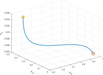
Figure 2: A trajectory of the state of the replicator dynamic equation in (25) with the initial state of $(x_{1},x_{2},x_{3})=(0.025,0.025,0.95)$ that is represented by $\circ$ marker, when $R=1$, $c=2$, $\Gamma=4$ (or 6 dB), $\bar{\gamma}=10$ (or 10 dB), $\mu=0.2$. The replicator dynamic converges to $(x_{1}^{*},x_{2}^{*},x_{3}^{*})=(0.035,0.415,0.550)$, which is represented by $\star$ marker.

Fig. 3 shows the results of the evolutionary game for hybrid uplink NOMA with different values of the scaling factor for cost, $c$, when $R=1$, $\Gamma=6$ dB, and $\bar{\gamma}=10$ dB. The ESS as a function of $c$ is shown in Fig. 3 (a), where we can see that $x_{1}^{*}$ decreases with $c$, which is expected by Property 5. That is, as the cost of transmission increases, users are not encouraged to use action 1. It can be also observed that $x_{1}=x_{2}\approx 0.46$ around $c=0.4$. This shows that the users choose action 1 or 2 equally likely so that a fair access can be achieved, while the maximum of throughput per user is obtained in Fig. 3 (b), where the throughput (per user) of hybrid uplink NOMA with is compared to that of OMA (i.e.,, TDMA). The throughput of OMA is given by $\frac{1-x_{3}}{2}$. We can observe that for a large cost of transmission (i.e., a large $c$), $x_{3}$ becomes high. In this case, the throughput of hybrid uplink NOMA is better than that of OMA as expected. That is, with a large threshold $\tau$ for truncated channel inversion power control (or a high $x_{3}$), it is better to share the channel with another user using NOMA to improve the throughput. Furthermore, with a sufficiently high $x_{3}$, as in [17] [31] [23], more than two users can be allocated to the same radio resource block.

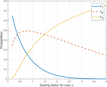
(a)

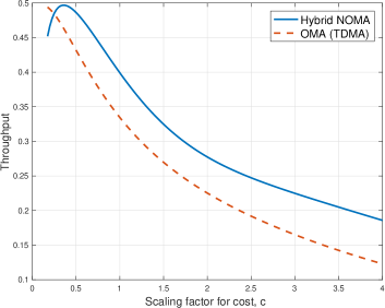
(b)

Figure 3: Evolutionary game for hybrid uplink NOMA with different values of the scaling factor for cost, $c$, when $R=1$, $\Gamma=4$ (i.e., 6 dB), and $\bar{\gamma}=10$ (i.e., 10 dB): (a) ESS as a function of $c$; (b) throughput per user.

We show the results of the evolutionary game for hybrid uplink NOMA with different values of average channel SNR, $\bar{\gamma}$, when $(R,c)=(1,1)$, $\Gamma=6$ dB, and $\bar{\gamma}=10$ dB in Fig. 4. In Fig. 4 (a), it is shown that $x_{1}^{*}$ increases with $\bar{\gamma}$ as expected by Property 5. That is, when $c$ is fixed, since the cost decreases with $\bar{\gamma}$, users are more encouraged to employ action 1 for a higher $\bar{\gamma}$. The throughput of hybrid uplink NOMA is shown in Fig. 4 (b), where we can see that hybrid uplink NOMA can have a higher throughput than OMA if $\bar{\gamma}$ is not too high.

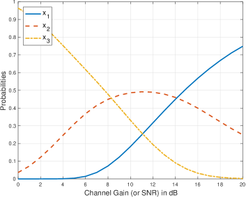
(a)

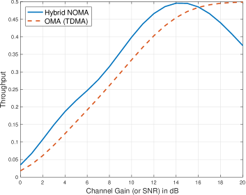
(b)

Figure 4: Evolutionary game for hybrid uplink NOMA with different values of average channel SNR, $\bar{\gamma}$ when $R=1$, $c=1$, and $\Gamma=4$ (i.e., 6 dB): (a) ESS as a function of $c$; (b) throughput per user.

As mentioned earlier, the ESS can be found using the replicator dynamic equation with the time averages of the rewards and costs as their estimates. To this end, in Subsection V-C, we have discussed the state updating rules at the BS and users, i.e., SU-BS and SU-U, respectively. Fig. 5 shows the trajectory of ${\bf x}$ obtained by the replicator dynamic equation in SU-BS when $M=300$, $\mu=0.5$, $B=40$, $\Gamma=6$ dB, $\bar{\gamma}=10$ dB, and $(R,c)=(1,1)$. Note that the initial ${\bf x}$ is set to $(1/3,1/3,1/3)$. In Fig. 5, the time for each iteration corresponds to one block interval (i.e., the duration of $B=40$ time slots). We can observe that SU-BS (using the replicator dynamic equation with the estimates of the average payoff that are obtained from time averages of the rewards and costs) can provide a good estimate of the ESS that is $(x_{1}^{*},x_{2}^{*},x_{3}^{*})=(0.183,0.486,0.331)$.

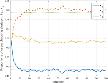
Figure 5: A trajectory of ${\bf x}$ obtained by the replicator dynamic equation in SU-BS when $M=300$, $\mu=0.5$, $B=40$, $\Gamma=6$ dB, $\bar{\gamma}=10$ dB, and $(R,c)=(1,1)$.

Unlike SU-BS, SU-U is a distributed state updating rule where each user updates the state and each user’ state can be different from the others. Thus, we show the average of $2M$ users’ states to show the trajectory of ${\bf x}$ in Fig. 6 where the state obtained by the replicator dynamic equation in SU-U is shown when $M=300$, $\mu=0.5$, $B=40$, $\Gamma=6$ dB, $\bar{\gamma}=10$ dB, and $(R,c)=(1,1)$. Compared with SU-BS in Fig. 6, SU-U has a slow convergence rate as it requires more iterations to converge to the ESS.

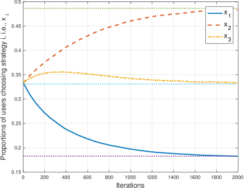
Figure 6: A trajectory of ${\bf x}$ obtained by the replicator dynamic equation in SU-U when $M=300$, $\mu=0.5$, $B=40$, $\Gamma=6$ dB, $\bar{\gamma}=10$ dB, and $(R,c)=(1,1)$.

Since the replicator dynamic equation can be seen as an adaptive updating rule for the state, it may be used when a parameter is varying over the time. For example, the control of the scaling factor for costs, $c$, might be necessary to improve the throughput as shown in Fig. 3 (b). In particular, the BS can broadcast a desirable value of $c$ to improve the overall performance. To see how the state can be updated with the replicator dynamic equation in SU-B, we consider the following variation of the scaling factor for costs for each block:

$$c[b]=\frac{2b}{200}+0.5,\ b=1,\ldots,200,$$ (39)

where $200$ is the number of blocks in a test. In Fig. 7, we show the trajectory of ${\bf x}$ by the replicator dynamic equation in SU-BS when $M=300$, $\mu=0.5$, $B=40$, $\Gamma=6$ dB, $\bar{\gamma}=10$ dB, and $R=1$. For comparisons, we also show the ESS with increasing $c[b]$ when the exact average payoffs are available. It is shown that the trajectory of ${\bf x}$ in SU-B can closely follow the ESS after some iterations.

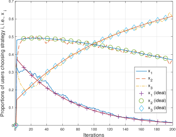
Figure 7: A trajectory of ${\bf x}$ obtained by the replicator dynamic equation in SU-BS and the ESS of ideal case (with the exact average payoffs) with time-varying scaling factor for costs when $M=300$, $\mu=0.5$, $B=40$, $\Gamma=6$ dB, $\bar{\gamma}=10$ dB, and $R=1$.

To see the trajectory of ${\bf x}$ in SU-U for varying $c$, we consider the variation of the scaling factor for costs for each block as follows:

$$c[b]=\frac{2b}{6000}+0.5,\ b=1,\ldots,6000,$$ (40)

where $6000$ is the number of blocks in a test. Note that the variation of $c$ in (40) is slower than that in (39) by a factor of $\frac{6000}{200}=30$. In Fig. 8, we show the trajectory of ${\bf x}$ by the replicator dynamic equation in SU-U when $M=300$, $\mu=0.5$, $B=40$, $\Gamma=6$ dB, $\bar{\gamma}=10$ dB, and $R=1$. When we compare the trajectory in SU-U with the ESS, it is clear that there is a time lag.

From Figs. 7 and 8, we can see that SU-BS can update the state faster than SU-U in accordance with the variation of $c$. Thus, SU-BS is preferable to SU-U when certain key parameters (e.g., $c$) are controlled by the BS for better performance at the cost of high signaling overhead.

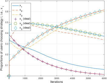
Figure 8: A trajectory of ${\bf x}$ obtained by the replicator dynamic equation in SU-U and the ESS of ideal case (with the exact average payoffs) with time-varying scaling factor for costs when $M=300$, $\mu=0.5$, $B=40$, $\Gamma=6$ dB, $\bar{\gamma}=10$ dB, and $R=1$.

VII Concluding Remarks

We proposed a hybrid uplink NOMA scheme to support more users using power-domain NOMA. In order to avoid high signaling overhead for the power allocation that is usually required for power-domain NOMA, truncated channel inversion power control at users was considered. The proposed hybrid uplink NOMA scheme was able to exploit fading in such a way that when one user does not transmit signals due to severe fading, another user can access the radio resource block. To decide the threshold values for the truncated channel inversion power control in hybrid uplink NOMA, an evolutionary game was formulated and its solution (i.e., ESS) was characterized. We also showed that the replicator dynamic equation can be used to find the ESS and discussed two implementation approaches to update the state with outcomes about the success of transmissions and realizations of fading channels.

Note that in this paper, we focused on the power control strategy for the hybrid uplink NOMA scheme based on power-domain NOMA. As in [32], there are other uplink NOMA schemes (e.g., sparse code multiple access (SCMA)). As a further research topic, the sparse code control (which might be equivalent to the power control) can be studied for SCMA from a point of view of evolutionary game theory. In addition, although we only consider two users per radio resource block in this paper, a generalization with more than two users per radio resource block is possible with more power levels. This generalization with a combination of power-domain NOMA and SCMA (to keep the maximum transmit power limited when there are a number of users per radio resource block) might be an interesting topic to be studied in the future.

Appendix A Proof of Property 1

For convenience, denote by ${\mathbb{P}}_{\bf x}(i)$ the probability that user 1 succeeds with action $i\in\{1,2\}$ when the state (or the mixed strategy) of user 2 is ${\bf x}$. Then, it can be shown that

$${\mathbb{P}}_{\bf x}(1)=x_{2}+x_{3}\ \mbox{and}\ {\mathbb{P}}_{\bf x}(2)=x_{1}+x_{3}.$$ (41)

In (41), we consider SIC to find ${\mathbb{P}}_{\bf x}(2)$. That is, although user 2 chooses action 1, user 1 can still succeed with action 2 using SIC. Since

$${\mathbb{E}}_{\bf x}[\mathbbm{1}({\rm succeed\ with\ action}\ i)]={\mathbb{P}}_{\bf x}(i),\ i\in\{1,2\},$$

we can show that

$$u_{1}(i,{\bf x})=R_{i}({\bf x})-\bar{C}_{i},\ i\in\{1,2\},$$ (42)

where

$$R_{i}({\bf x})=\left\{\begin{array}[]{ll}R(x_{2}+x_{3}),&\mbox{if $i=1$}\cr R(x_{1}+x_{3}),&\mbox{if $i=2$.}\cr\end{array}\right.$$ (45)

Substituting (42) into the first equation in (9), we can have the second equation in (9) after some manipulations. This completes the proof.

Appendix B Proof of Property 2

With a slight abuse of notation, let $u_{k}(i,j)$ denote the payoff of user $k$ when user 1 and user 2 choose pure strategies, $i$ and $j$. In addition, if user 1 chooses a mixed strategy ${\bf x}$ and user 2 chooses a mixed strategy ${\bf x}^{\prime}$, the payoff of user $k$ is denoted by $u_{k}({\bf x},{\bf x}^{\prime})$. If user 2 chooses a mixed strategy ${\bf x}$ and user 1 chooses a pure strategy $i$, then the payoff of user 1 is denoted by $u_{1}(i,{\bf x})$, which is identical to that in (6). By the definition of a mixed strategy NE [20] we have

$$u_{1}(i,{\bf x}^{*})\leq u_{1}({\bf x}^{*},{\bf x}^{*}),\ i\in\{1,2,3\},$$ (46)

if ${\bf x}^{*}$ is a mixed strategy NE. Note that since the game is symmetric, (46) is equivalent to $u_{2}({\bf x}^{*},i)\leq u_{2}({\bf x}^{*},{\bf x}^{*}),\ i\in\{1,2,3\}$. From (9), it can be readily shown that

$$u_{1}({\bf x}^{*},{\bf x})=u({\bf x}^{*},{\bf x}^{*}).$$ (47)

Substituting (47) into (46), we can have (12), which completes the proof.

Appendix C Proof of Property 3

In case of A, according to the indifference principle [20], we have

$$u_{1}(1,{\bf x}^{*})=u_{1}(2,{\bf x}^{*})=u_{1}(3,{\bf x}^{*}).$$ (48)

Since $x_{1}^{*}+x_{2}^{*}+x_{3}^{*}=1$, from (48), we have

$$Rx_{1}^{*}-R+C_{1}=Rx_{2}^{*}-R+C_{2}=0.$$

This leads to (13) as $C_{1}<R$ and $C_{1}+C_{2}>R$.

In case of B, we can see that $x_{1}^{*}$ has to be zero, while $x_{2}^{*},x_{3}^{*}>0$. According to the indifference principle [20], we need to have $u_{1}(2,{\bf x}^{*})=u_{1}(3,{\bf x}^{*})$, which results in (14).

In case of C, since costs $C_{1}$ and $C_{2}$ are higher than reward $R$, $x_{1}^{*}$ and $x_{2}^{*}$ become 0 and $x_{3}^{*}=1$, which means that no transmission becomes NE.

In case of D, we can see that $u_{1}(1,{\bf x})=u_{1}(2,{\bf x})$ with $x_{3}^{*}=0$, which leads to (16) and completes the proof.

Appendix D Proof of Property 4

From (17), the probability density function (pdf) of $\gamma_{k}$ is given by $f_{\gamma}(\gamma_{k})=\frac{1}{\bar{\gamma}}e^{-\frac{\gamma_{k}}{\bar{\gamma}}}$. Using this, we can show that

$$\bar{C}_{1} =c\rho_{1}{\mathbb{E}}\left[\frac{1}{\gamma_{k}}\,|\,\gamma_{k}\in{\cal G}_{1}\right]$$ (49)

$$=c\rho_{1}\int_{0}^{\infty}\frac{1}{\gamma}f_{\gamma}(\gamma\,|\,\gamma\in{\cal G}_{1})d\gamma$$ (50)

$$=\frac{c\rho_{1}}{x_{1}}\int_{\tau_{\rm pn}}^{\infty}\frac{1}{\gamma}f_{\gamma}(\gamma)d\gamma=\frac{c\rho_{1}}{\bar{\gamma}x_{1}}E_{1}\left(\frac{\tau_{\rm pn}}{\bar{\gamma}}\right).$$ (51)

Similarly, we can also derive that

$$\bar{C}_{2}=\frac{c\rho_{2}}{\bar{\gamma}x_{2}}\left(E_{1}\left(\frac{\tau}{\bar{\gamma}}\right)-E_{1}\left(\frac{\tau_{\rm pn}}{\bar{\gamma}}\right)\right).$$ (52)

Furthermore, from (17) and (5), we can readily show that

$$\tau =\bar{\gamma}\ln\frac{1}{1-x_{3}}=\bar{\gamma}\ln\frac{1}{x_{1}+x_{2}}$$ (53)

$$\tau_{\rm pn} =\bar{\gamma}\ln\frac{1}{x_{1}}.$$ (54)

Substituting (54) into (51) and (52), we have the costs in (21), which completes the proof.

Appendix E Proof of Property 5

Since $x_{3}>0$, based on the indifference principle, we need to have $u_{1}(1,{\bf x})=0$ or from (45) and (21),

$$R(x_{2}+x_{3})-\bar{C}_{1}({\bf x})=R(1-x_{1})-\bar{C}_{1}({\bf x})=0,$$

which leads to (22). Consider $V(x)=\frac{E_{1}\left(\ln\frac{1}{x}\right)}{x}$, $x\in(0,1)$. It can be shown that

$$\lim_{x\to 0}V(x)=\lim_{x\to 0}\frac{\frac{1}{x}E_{0}(-\ln x)}{1}=0,$$ (55)

where the limit is due to L’Hospital’s rule, the fact that $\frac{d}{dx}E_{n}(x)=-E_{n-1}(x)$ (for $n=0,1\ldots$), and $E_{0}(x)=-\frac{e^{-x}}{x}$. In addition, let $\tilde{V}=V(\tilde{x}_{3})$. It can be shown that

$$\frac{dV(x)}{dx} =-\frac{1}{x\ln x}-\frac{E_{1}(-\ln x)}{x^{2}}$$ (56)

$$=\frac{1}{x}\left(-\frac{1}{\ln x}-\frac{E_{1}(-\ln x)}{x}\right)$$ (57)

$$\geq\frac{1}{x}\left(-\frac{1}{\ln x}-\ln\left(1-\frac{1}{\ln x}\right)\right)>0,$$ (58)

where the first inequality is due to $E_{1}(x)\leq e^{-x}\ln\left(1+\frac{1}{x}\right)$, $x\geq 0$, and the second inequality is due to $z>\ln(1+z)$, $z>0$, with $z=-\frac{1}{\ln x}>0$. Since $C_{1}({\bf x})=\frac{c\rho_{1}}{\bar{\gamma}}V(x)$, $C_{1}({\bf x})$ is an increasing function of $x_{1}$ and $\lim_{x_{1}\to 0}C_{1}({\bf x})=0$ and

$$C_{1}({\bf x})\bigl{|}_{x_{1}=\tilde{x}_{3}}=\frac{c\rho_{1}}{\bar{\gamma}}\tilde{V},$$

while $R(1-x_{1})$ is a decreasing function of $x_{1}$. As a result, (22) has a unique solution if $\frac{c\rho_{1}}{\bar{\gamma}}\tilde{V}>Rx_{3}$, which is equivalent to (23).

Furthermore, since $C_{1}({\bf x})$ increases with $c$ and decreases with $\bar{\gamma}$, we can also see that $x_{1}^{*}$ decreases with $c$ and increases with $\bar{\gamma}$.

References

- [1] L. Dai, B. Wang, Y. Yuan, S. Han, C. I, and Z. Wang, “Non-orthogonal multiple access for 5G: solutions, challenges, opportunities, and future research trends,” IEEE Communications Magazine, vol. 53, pp. 74–71, September 2015.
- [2] Z. Ding, Y. Liu, J. Choi, M. Elkashlan, C. L. I, and H. V. Poor, “Application of non-orthogonal multiple access in LTE and 5G networks,” IEEE Communications Magazine, vol. 55, pp. 185–191, February 2017.
- [3] J. Choi, “NOMA: Principles and recent results,” in 2017 International Symposium on Wireless Communication Systems (ISWCS), pp. 349–354, Aug 2017.
- [4] L. Dai, B. Wang, Z. Ding, Z. Wang, S. Chen, and L. Hanzo, “A survey of non-orthogonal multiple access for 5g,” IEEE Communications Surveys Tutorials, vol. 20, pp. 2294–2323, thirdquarter 2018.
- [5] Y. Saito, Y. Kishiyama, A. Benjebbour, T. Nakamura, A. Li, and K. Higuchi, “Non-orthogonal multiple access (NOMA) for cellular future radio access,” in Vehicular Technology Conference (VTC Spring), 2013 IEEE 77th, pp. 1–5, June 2013.
- [6] B. Kim, S. Lim, H. Kim, S. Suh, J. Kwun, S. Choi, C. Lee, S. Lee, and D. Hong, “Non-orthogonal multiple access in a downlink multiuser beamforming system,” in MILCOM 2013 - 2013 IEEE Military Communications Conference, pp. 1278–1283, Nov 2013.
- [7] Y. Sun, Z. Ding, and X. Dai, “On the performance of downlink NOMA in multi-cell mmwave networks,” IEEE Communications Letters, vol. 22, pp. 2366–2369, Nov 2018.
- [8] Z. Xiao, L. Zhu, J. Choi, P. Xia, and X. Xia, “Joint power allocation and beamforming for non-orthogonal multiple access (NOMA) in 5G millimeter wave communications,” IEEE Trans. Wireless Communications, vol. 17, pp. 2961–2974, May 2018.
- [9] J. Choi, “Non-orthogonal multiple access in downlink coordinated two-point systems,” IEEE Commun. Letters, vol. 18, pp. 313–316, Feb. 2014.
- [10] W. Shin, M. Vaezi, B. Lee, D. J. Love, J. Lee, and H. V. Poor, “Coordinated beamforming for multi-cell MIMO-NOMA,” IEEE Communications Letters, vol. 21, pp. 84–87, Jan 2017.
- [11] Y. Sun, Z. Ding, X. Dai, and G. K. Karagiannidis, “A feasibility study on network NOMA,” IEEE Trans. Communications, vol. 66, pp. 4303–4317, Sep. 2018.
- [12] Y. Sun, Z. Ding, X. Dai, and O. A. Dobre, “On the performance of network NOMA in uplink CoMP systems: A stochastic geometry approach,” IEEE Trans. Communications, pp. 1–1, 2019.
- [13] M. Al-Imari, P. Xiao, M. A. Imran, and R. Tafazolli, “Uplink non-orthogonal multiple access for 5G wireless networks,” in 2014 11th International Symposium on Wireless Communications Systems (ISWCS), pp. 781–785, Aug 2014.
- [14] N. Zhang, J. Wang, G. Kang, and Y. Liu, “Uplink nonorthogonal multiple access in 5G systems,” IEEE Communications Letters, vol. 20, pp. 458–461, March 2016.
- [15] J. Choi, “Joint rate and power allocation for NOMA with statistical CSI,” IEEE Trans. Communications, vol. 65, pp. 4519–4528, Oct 2017.
- [16] Y. Liu, M. Derakhshani, and S. Lambotharan, “Outage analysis and power allocation in uplink non-orthogonal multiple access systems,” IEEE Communications Letters, vol. 22, pp. 336–339, Feb 2018.
- [17] J. Choi, “NOMA-based random access with multichannel ALOHA,” IEEE J. Selected Areas in Communications, vol. 35, pp. 2736–2743, Dec 2017.
- [18] J. Choi, “Layered non-orthogonal random access with SIC and transmit diversity for reliable transmissions,” IEEE Trans. Communications, vol. 66, pp. 1262–1272, March 2018.
- [19] D. Fudenberg and J. Tirole, Game Theory. Cambridge, MA: MIT Press, 1991.
- [20] M. Maschler, S. Zamir, and E. Solan, Game Theory. Cambridge University Press, 2013.
- [21] J. Choi, “Multichannel NOMA-ALOHA game with fading,” IEEE Trans. Communications, vol. 66, pp. 4997–5007, Oct 2018.
- [22] J. Seo and H. Jin, “Two-user NOMA uplink random access games,” IEEE Communications Letters, vol. 22, pp. 2246–2249, Nov 2018.
- [23] J. Seo, T. Kwon, and J. Choi, “Evolutionary game approach to uplink NOMA random access systems,” IEEE Communications Letters, pp. 1–1, 2019.
- [24] Z. Ding, R. Schober, P. Fan, and H. V. Poor, “Simple semi-grant-free transmission strategies assisted by non-orthogonal multiple access,” IEEE Trans. Communications, pp. 1–1, 2019.
- [25] A. Goldsmith and P. Varaiya, “Capacity of fading channels with channel side information,” IEEE Trans. Inform. Theory, vol. 43, pp. 1986–1992, Nov. 1997.
- [26] D. Tse and P. Viswanath, Fundamentals of Wireless Communication. Cambridge University Press, 2005.
- [27] J. Choi, “On power and rate allocation for coded uplink NOMA in a multicarrier system,” IEEE Trans. Communications, vol. 66, pp. 2762–2772, June 2018.
- [28] J. Weibull, Evolutionary Game Theory. Evolutionary Game Theory, MIT Press, 1995.
- [29] S. Timotheou and I. Krikidis, “Fairness for non-orthogonal multiple access in 5G systems,” IEEE Signal Process. Letters, vol. 22, pp. 1647–1651, Oct 2015.
- [30] J. Choi, “Power allocation for max-sum rate and max-min rate proportional fairness in NOMA,” IEEE Commun. Letters, vol. 20, pp. 2055–2058, Oct 2016.
- [31] J. Choi, “Multichannel NOMA-ALOHA game with fading,” IEEE Trans. Communications, vol. 66, pp. 4997–5007, Oct 2018.
- [32] Y. Chen, A. Bayesteh, Y. Wu, B. Ren, S. Kang, S. Sun, Q. Xiong, C. Qian, B. Yu, Z. Ding, S. Wang, S. Han, X. Hou, H. Lin, R. Visoz, and R. Razavi, “Toward the standardization of non-orthogonal multiple access for next generation wireless networks,” IEEE Communications Magazine, vol. 56, pp. 19–27, March 2018.