An empirical comparison between stochastic and deterministic centroid initialisation for K-Means variations

Abstract

K-Means is one of the most used algorithms for data clustering and the usual clustering method for benchmarking. Despite its wide application it is well-known that it suffers from a series of disadvantages; it is only able to find local minima and the positions of the initial clustering centres (centroids) can greatly affect the clustering solution. Over the years many K-Means variations and initialisation techniques have been proposed with different degrees of complexity. In this study we focus on common K-Means variations along with a range of deterministic and stochastic initialisation techniques. We show that, on average, more sophisticated initialisation techniques alleviate the need for complex clustering methods. Furthermore, deterministic methods perform better than stochastic methods. However, there is a trade-off: less sophisticated stochastic methods, executed multiple times, can result in better clustering. Factoring in execution time, deterministic methods can be competitive and result in a good clustering solution. These conclusions are obtained through extensive benchmarking using a range of synthetic model generators and real-world data sets.

Keywords K-Means clustering  $\cdot$ Deterministic clustering  $\cdot$ Benchmarking

1 Introduction

The most well-known algorithm in the field of clustering analysis is the K-Means algorithm. Its simplicity, versatility and efficiency makes it popular in many different research fields [1, 2]. Despite its reputation and success in many different studies, it has a series of disadvantages such that it can detect only spherical and well-separated clusters, it is sensitive to outliers, highly dependent on the features (dimensions) of the data set and it only converges to local minima [2]. Over the years a number of K-Means variations (Lloyd’s K-Means [3], Hartigan-Wong’s K-Means [4]), K-Means inspired algorithms (K-Medians [5]), and K-Means initialisation methods [6] have been proposed in order to overcome some of these issues. Such methods have also enhanced KMeans with additional properties such as feature selection mechanisms [7, 8], semi-supervised capabilities [9, 10], and outliers robustification [11, 12].

In the literature there are various studies regarding the importance of the initial selection of cluster centroids for the performance of the K-Means algorithm [2] and extensive testing on various initialisation techniques [6, 13], but a detailed comparison on the effects on these techniques on common K-Means variations is not available. We hypothesize that sophisticated initialisation methods alleviate the need for complex clustering and, if deterministic, they could lead to satisfactory solutions within a single execution of the clustering algorithm. Consequently, they would alleviate the need for executing a stochastic method multiple times and picking the best clustering based on some criterion.

In order to investigate this hypothesis we compare different clustering initialisation methods, namely Random [14], K-Means++ [15], Maximin [16] ROBust INitialisation (ROBIN) [11], Kaufman [17] and Density K-Means++ (DK-Means++) [18], and their effects on common K-Means variations, Lloyd’s K-Means [2], Hartigan-Wong’s K-Means [19, 4] and K-Medians [5]. We show that more sophisticated initialisation methods reduce on average the performance difference among the K-Means implementations and that the deterministic DK-Means++ method can achieve better average performance than stochastic methods. Nevertheless there is a trade-off, simplistic stochastic methods can achieve better clustering performance if executed multiple times due to the potential of discovering better local minima. For very large data sets where execution time is a factor, a single run using a deterministic initialisation method can be competitive compared to multiple runs using stochastic initialisation methods. A similar study comparing many different intialisation methods has been performed by [6] but it is focused on algorithms of linear complexity without considering various K-Means implementations. Recently, another study [13] was performed on stochastic initialization heuristics for K-Means and on how much the algorithm can be improved by repetition. They based their conclusions on a clustering benchmark [20, 13] which contains standalone data sets with different properties and they showed that K-Means performance is in general poor on unbalanced data sets and that the algorithm is not affected by high dimensionality while more iterations can improve its performance on overlapping clusters. In our case we performed a more extensive benchmarking by taking into consideration data set generation models as well as standalone data sets. The models gave us the ability to perform hypothesis testing in order to strengthen our conclusions and to account for variability.

The code of the clustering methods, data set model generators, scripts and a standalone application to reproduce this research are available in the GitHub repository https://github.com/avouros/Code-KMeans-benchmark (under the branch additions).

2 Material and method

2.1 The K-Means algorithm

Given K initial centroids, the K-Means algorithm [2] assigns the data points into $K$ clusters in a way that minimizes the within cluster sum of squares (WCSS):

$$WCSS =\sum_{k=1}^{K}\sum_{\binom{i=1}{x_{i:}\in c_{k}}}^{n_{k}}\sum_{j=1}^{p}(x_{ij}-m_{kj})^{2},$$ (1)

where $K$ is the number of clusters, $n_{k}$ the number of data points (observations) of the $k$-th cluster and $p$ the dimensionality (number of features) of a given dataset; $x_{ij}$ is the value of the $j$-th feature of the $i$-th data point, $x_{i:}$ is the vector representing the $i$-th datapoint; $m_{k:}$ specifies the location of the $k\text{-}th$ cluster centroid. This problem is equivalent to maximizing the between cluster sum of squares (BCSS) which is given by [7]:

$$BCSS =\sum_{j=1}^{p}\bigg{(}\sum_{i=1}^{n}(x_{ij}-\mu_{1j})^{2}-\sum_{k=1}^{K}\sum_{\binom{i=1}{x_{i:}\in c_{k}}}^{n_{k}}(x_{ij}-m_{kj})^{2}\bigg{)},$$ (2)

where $\mu_{1:}$ specifies the global centroid assuming that all the data points belong to one cluster.

2.1.1 Lloyd’s K-Means

Lloyd’s method is the most commonly used K-Means and the standard K-Means clustering method in many programming languages such as MATLAB [21] and Python [22]. The steps of this algorithm are as follows [2]:

1. Initialise $K$ initial centroids $m_{1j},\dots,m_{Kj}$ using some initialisation method.

2. Assign each data point $x_{i:}$ to cluster $c_{k^{*}}$,

   $$k^{*} =\underset{k}{argmin}\bigg{\{}\sum_{j=1}^{p}(x_{ij}-m_{kj})^{2}\bigg{\}}.$$ (3)

3. Recompute each cluster centroid using the formula,

   $$m_{kj}=\frac{\sum_{\binom{i=1}{x_{i:}\in c_{k}}}^{n_{k}}x_{ij}}{n_{k}}.$$ (4)

4. Go to step 2 until converge.

2.1.2 Hartigan-Wong’s K-Means

Hartigan-Wong’s K-Means algorithm is an alternative to Lloyd’s K-Means and the default K-Means of the R language [23]. In the study of [3] it is shown that this method has lower probability of converging to a local minima solution compared to Lloyd’s method in exchange of extra complexity. The steps of the algorithm are as follows [4, 3]:

1. Initialise $K$ initial centroids $m_{1j},\dots,m_{Kj}$ using an initialisation method.

2. Assign each data point $x_{i:}$ to cluster $c_{k^{\prime}}$,

   $$k^{\prime} =\underset{k}{argmin}\bigg{\{}\sum_{j=1}^{p}(x_{ij}-m_{kj})^{2}\bigg{\}}.$$

3. Set an indicator $s=1$.

4. For each data point $x_{i:}$

   1. Remove it from its cluster $c_{k^{\prime}}$.

   2. Compute the centroid of $c_{k^{\prime}}$ using the remaining points in that cluster,

      $$m_{k^{\prime}j}=\frac{1}{n_{k^{\prime}}}\sum_{\binom{i=1}{x_{i:}\in c_{k^{\prime}}}}^{n_{k^{\prime}}}x_{ij}.$$

   3. Assign $x_{i:}$ to cluster $c_{k^{*}}$,

      $$k^{*} =\underset{k}{argmin}\bigg{\{}\sum_{j=1}^{p}(x_{ij}-m_{kj})^{2}\bigg{\}}.$$

   4. Recompute the centroid of the cluster $c_{k^{*}}$,

      $$m_{k^{*}j}=\frac{1}{n_{k^{*}}}\sum_{\binom{i=1}{x_{i:}\in c_{k^{*}}}}^{n_{k^{*}}}x_{ij}.$$

   5. If $k^{*}\neq k^{\prime}$ set $s=0$.

5. If $s=0$, set $s=1$ and go to step 4.

2.1.3 The K-Medians algorithm

The K-Medians algorithm [5] is similar to the K-Means but uses the median instead of the mean to calculate the cluster centroid. The objective function of the algorithm is given by the equation:

$$E =\sum_{k=1}^{K}\sum_{\binom{i=1}{x_{i:}\in c_{k}}}^{n_{k}}\sum_{j=1}^{p}|x_{ij}-\bar{m}_{kj}|,$$ (5)

where $\bar{m}_{kj}$ specifies the location of the $k\text{-}th$ cluster centroid in the $j$-th dimension which is computed by taking the median of the data points $x_{ij}$ belonging to that cluster. K-Medians corresponds to the $L_{1}$-norm as opposed to the $L_{2}$-norm of K-Means [5]. The use of median in place of the mean makes the K-Medians algorithm robust to outliers [24, 25] since the median has a breaking point of 0.5, i.e. even if half of the data set is corrupted by outliers the median of the corrupted data set will be similar to the median of the original data set [26]. The common implementation of the algorithm is similar to Lloyd’s K-Means where, in the $3rd$ step of Lloyd’s algorithm, the median is used to compute the new centroids locations instead of the mean., i.e. $\forall\hphantom{x}k$ $\bar{m}_{k:}=median(\{x_{i:}\}),\hphantom{x}x_{i:}\in c_{k}$.

2.2 K-Means initialisation methods

Let $D(x_{i:})$ denote the distance between data point $x_{i:}$ and the nearest of the selected cluster centroids, $m_{k:}$, $k=1,\dots,L$, with $L$ being the number of selected centroids ($L\leq K$):

$$D(x_{i:})=\underset{k}{min}\sqrt{\sum_{j=1}^{p}(x_{ij}-m_{kj})^{2}}.$$ (6)

2.2.1 Random

The initialisation method of MacQueen [14] proposes a random selection of data points from the data set which will be the initial centroids. This is one of the earliest clustering initialisation techniques and an improvement of Jancey’s method [27]. The latter study suggested the centroids to be at random locations within the minimum hypersphere of the data set but this might result in empty clusters to be generated after the execution of the K-Means algorithm.

2.2.2 K-Means++

K-Means++ [15] is a standard clustering initialisation technique in many programming languages such as MATLAB and Python. It has linear complexity $\mathcal{O}(N)$ and it uses a probabilistic approach in order to select as initial centroids data points that are far away from each other. The steps of this algorithm are as follows:

1. Select randomly a data point $x_{i:}$ as the first centroid $m_{1:}$ and set $k=2$.

2. Choose another data point $x_{i^{\prime}:}$ as the next centroid $m_{k:}$ with probability

   $$p(x_{i^{\prime}:})=\frac{D(x_{i^{\prime}:})^{2}}{\sum_{i=1}^{n}D(x_{i:})^{2}}$$

   and set $k=k+1$.

3. While $k\leq K$ go to step 2.

2.2.3 Maximin

The maximin method of [16] picks data points as cluster centroids that are far apart form each other.

1. Select randomly a data point $x_{i:}$ as the first centroid $m_{1:}$ and set $k=2$.

2. Select as the next centroid $m_{k:}=x_{i^{\prime}:}$ with $i^{\prime}=\underset{i}{argmax}\{D(x_{i:})\}$ and set $k=k+1$.

3. While $k\leq K$ go to step 2.

Maximin has linear complexity $\mathcal{O}(N)$. The study of [28] proposed a modification in the first step of the algorithm to select as the first centroid the data point with the maximum Euclidean norm [6]. In this way the method can become deterministic.

2.2.4 Kaufman

Kaufman and Rousseeuw [17] proposed a deterministic method for centroids initialisation. Their method is as follows [1]:

1. Select the closest data point to the global centroid of the data set as the first centroid $m_{1:}$ and set $k=2$.

2. For every two non-selected data points $x_{i:}$ and $x_{i^{\prime}:}$ calculate,

   $$C_{i^{\prime}i}=max\Bigg{\{}D(x_{i:})-\sqrt{\sum_{j=1}^{p}(x_{ij}-x_{i^{\prime}j})^{2}},0\Bigg{\}}.$$

3. Select as the next centroid $m_{k:}=x_{i^{*}:}$, with $i^{*}=\underset{i}{argmax}\{\sum_{i^{\prime}}C_{i^{\prime}i}\}$ and set $k=k+1$.

4. While $k\leq K$ go to step 2.

Kaufman’s and Rousseeuw’s algorithm has quadratic complexity $\mathcal{O}(N^{2})$ because of the computation of the pairwise distances [6].

2.2.5 ROBust INitialisation (ROBIN)

ROBIN [11] is a robust to outliers initialisation method. It uses the Local Outlier Factor (LOF) [29] in order to select as initial centroids data points that are far away from each other and also representative points of dense regions in the data set. In addition it requires one more tuning parameter which is the number of neighboring data points $mp$ to be consider when computing the LOF of each data point. The LOF score of each data point, $LOF(x_{i:},mp)$, is given by the algorithm below [11] (where $N(x_{i:},mp)$ is the set of the $mp$ nearest data points to the $x_{i,:}$ data point, with $|N(x_{i:},mp)|\geq mp$):

1. Compute the density of each data point $x_{i:}$,

   $$density(x_{i:},mp)=\frac{|N(x_{i:},mp)|}{\sum_{x_{i^{\prime}:}\in N(x_{i:},mp)}\sqrt{\sum_{j=1}^{p}(x_{ij}-x_{i^{\prime}j})^{2}}},i\neq i^{\prime}.$$ (7)

2. Compute the average relative density of each data point $x_{i:}$,

   $$ard(x_{i:},mp)=\frac{density(x_{i:},mp)}{\frac{\sum_{x_{i^{\prime}:}\in N(x_{i:},mp)}density(x_{i^{\prime}:},mp)}{|N(x_{i:},mp)|}}.$$ (8)

3. Compute the LOF score of each data point $x_{i:}$,

   $$LOF(x_{i:},mp)=\frac{1}{ard(x_{i:},mp)}.$$ (9)

The ROBIN algorithm ($K>1$ ) is described below [11]:

1. Pick a reference data point $x_{r:}$ from the data set.

2. Sort the data points in decreasing order of their distance from $x_{r:}$.

3. For each $x_{i:}$ in sorted order, pick the first data point $x_{i^{\prime}:}$ for which
   $LOF(x_{i^{\prime}:},mp)\approx 1$ as the first centroid $m_{1:}$ and set $k=2$.

4. Sort the data points in decreasing order based on $D(x_{i:})$. For the formula of $D(x_{i:})$ refer to equation 6.

5. For each $x_{i:}$ in sorted order, pick the first data point $x_{i^{\prime}:}$ for which
   $LOF(x_{i^{\prime}:},mp)\approx 1$ as the next centroid $m_{k:}$ and set $k=k+1$.

6. While $k\leq K$ go to step 4.

The computational cost of this method is dominated by the complexity of sorting, which is $\mathcal{O}(N\textit{ log }N)$ [6] but for the LOF score calculation we have a choice of algorithms varying from $\mathcal{O}(N)$ to $\mathcal{O}(N^{2})$, that can be chosen based on dimensionality-related constraints, see [29]. Regarding the $4^{th}$ step of the algorithm, in an R implementation (refer to the study of [12]) the formula $LOF(x_{r^{\prime}:},mp)<1.05$ was used but since the LOF score can also be lower than $1$, in our experiments, we used the formula $1-e<LOF(x_{r^{\prime}:},mp)<1+e$ where $e$ was set to $0.05$. In the original algorithm [11] the authors are using the algorithm in a deterministic manner by setting the reference point on step 2, $x_{r}:$ to the origin. In the $R$ implementation of [12] the reference point is chosen at random. In this study we test both methods, ROBIN(S) will refer to the stochastic method of [12] while ROBIN(D) will refer to the deterministic method of [11].

2.2.6 Density K-Means++ (DK-Means++)

DK-Means++ [18] is a deterministic method for centroids initialisation based on data density. It is an improved method of [30, 31] since it requires only to define the number of clusters $K$ and utilizes a heuristic to detect dense regions in the data set based on a radius $\varepsilon$ in order to select optimal centroids. The radius $\varepsilon$ can be computed form the following algorithm [18]:

1. Construct the minimum spanning tree of the distance matrix of the data set.

2. Let $\Lambda$ be the weights of edges of the Minimum Spanning Tree and IQR the Inter Quartile Range. Then,

   $$\varepsilon=3\cdot IQR(\Lambda)+75^{th}percentile(\Lambda).$$

The DK-Means++ algorithm is described below [18]:

1. Compute the the local density $p(x_{i:})$ of each data point using the formula:

   $$p(x_{i:})=\sum_{x_{i^{\prime}}\in\varepsilon\text{-}neighbors(x_{i:})}\exp\Bigg{(}\frac{-\sqrt{\sum_{j=1}^{p}(x_{ij}-x_{i^{\prime}j})^{2}}}{\varepsilon}\Bigg{)}.$$

   where $\varepsilon\text{-}neighbors(x_{i:})$ are the data points falling under the hypersphere with centroid $x_{i:}$ and radius $\varepsilon$.

2. Normalize $p(x_{i:})$ using the min-max normalization.

3. The first cluster centroid $m_{1:}$ is the data point $x_{i^{*}:}$ for which $p(x_{i^{*}:})=max\{p(x)\}$. Then $m_{1:}=x_{i^{*}:}$ and $k=2$.

4. Compute the prospectiveness all data points that are not selected as centers given the formula, $\phi(x_{i:})=p(x_{i:})\cdot D(x_{i:})$. For the formula of $D(x_{i:})$ refer to equation 6.

5. The next centroid $m_{k:}$ is the data point with maximum prospectiveness: $m_{k:}=x_{i^{*}:}$ with $i^{*}=\underset{i}{argmax}\{\phi(x_{i:})\}$ and $k=k+1$.

6. While $k\leq K$ go to step 4.

The computation of $\varepsilon\text{-}neighbors$ contributes to the complexity of DK-Means++. It is dominated by the distance matrix computation, which is $O(n^{2})$. The computation of the Minimum Spanning Tree depends of the algorithm used to compute it, efficient implementations of Kruskal’s algorithm and Prim’s algorithm require $O$($n$ log $n$) time to compute a minimum spanning tree [32]. As $O(n^{2})$ is the dominating complexity, the entire process of finding initial centroids, of DK-Means++ has a time complexity of $O(n^{2})$.

2.3 Clustering evaluation

In the literature there are many indexes for assessing the clustering performance [11, 33, 20]. Here, in order to evaluate the clustering solutions, we selected to use one external (supervised) criterion, the Purity and one internal (unsupervised) criterion, the Silhouette index.

2.3.1 Purity

Let our data belong to different classes $\ell_{\mathsf{k}}$ and that the number of classes $\mathsf{K}$ equals the number of clusters $K$, for each cluster the purity is defined as [33],

$$P_{c_{k}}=\frac{1}{n_{k}}\underset{\mathsf{k}}{max}\{n_{\ell_{\mathsf{k}}}^{(k)}\},$$ (10)

where $\underset{\mathsf{k}}{max}\{n_{\ell_{\mathsf{k}}}^{(k)}\}$ specifies the number of data points of the dominant class of the $k$-th cluster. The overall clustering purity index is then computed as,

$$P=\sum_{i=1}^{K}\frac{n_{k}}{n}P_{c_{k}}.$$ (11)

The purity index is bounded between $(0\text{ }1]$; larger values of purity correspond to better performance accuracy and a purity of $1$ specifies an accuracy of $100\%$ meaning that each cluster has data points from only one class.

2.3.2 Silhouette index

The silhouette index is a value that specifies the degree of similarity between a data point and other data points of the same cluster and the dissimilarity between a data point and other data points in different clusters. The silhouette index of the data point $x_{i:}\in c_{k}$ is given by 12 [34],

$$S_{x_{i:}}=\frac{b_{x_{i:}}-a_{x_{i:}}}{max\{b_{x_{i:}},a_{x_{i:}}\}},$$ (12)

where $a_{x_{i:}}$ is the average distance of $x_{i:}$ and all the other data points in the cluster that $x_{i:}$ belongs to

$$a_{x_{i:}}=\frac{1}{n_{k}-1}\sum_{\binom{i^{\prime}=1}{x_{i^{\prime}:}\in c_{k}}}^{n_{k}}\sqrt{\sum_{j=1}^{p}(x_{ij}-x_{i^{\prime}j})^{2}}$$ (13)

and $b_{x_{i:}}$ is the minimum average distance of $x_{i:}$ to all the other data points in other clusters,

$$b_{x_{i:}}=\underset{k^{\prime}}{min}{\frac{1}{n_{k^{\prime}}}\sum_{\binom{i^{\prime}=1}{x_{i^{\prime}:}\in c_{k^{\prime}}}}^{n_{k^{\prime}}}\sqrt{\sum_{j=1}^{p}(x_{ij}-x_{i^{\prime}j})^{2}},k^{\prime}\neq k}.$$ (14)

We can then define the average silhouette index,

$$S=\frac{1}{n}\sum_{i=1}^{n}S_{x_{i:}}.$$ (15)

The silhouette index is commonly used to estimate the number of clusters in a data set but it can also be used to assess the clustering quality [34]. The Silhouette index is bounded between $-1$ and $1$, where $1$ specifies maximum separation of clusters and maximum within cluster density while other indexes, such as the distortion score, gives only an estimation of the latter.

3 Benchmarks

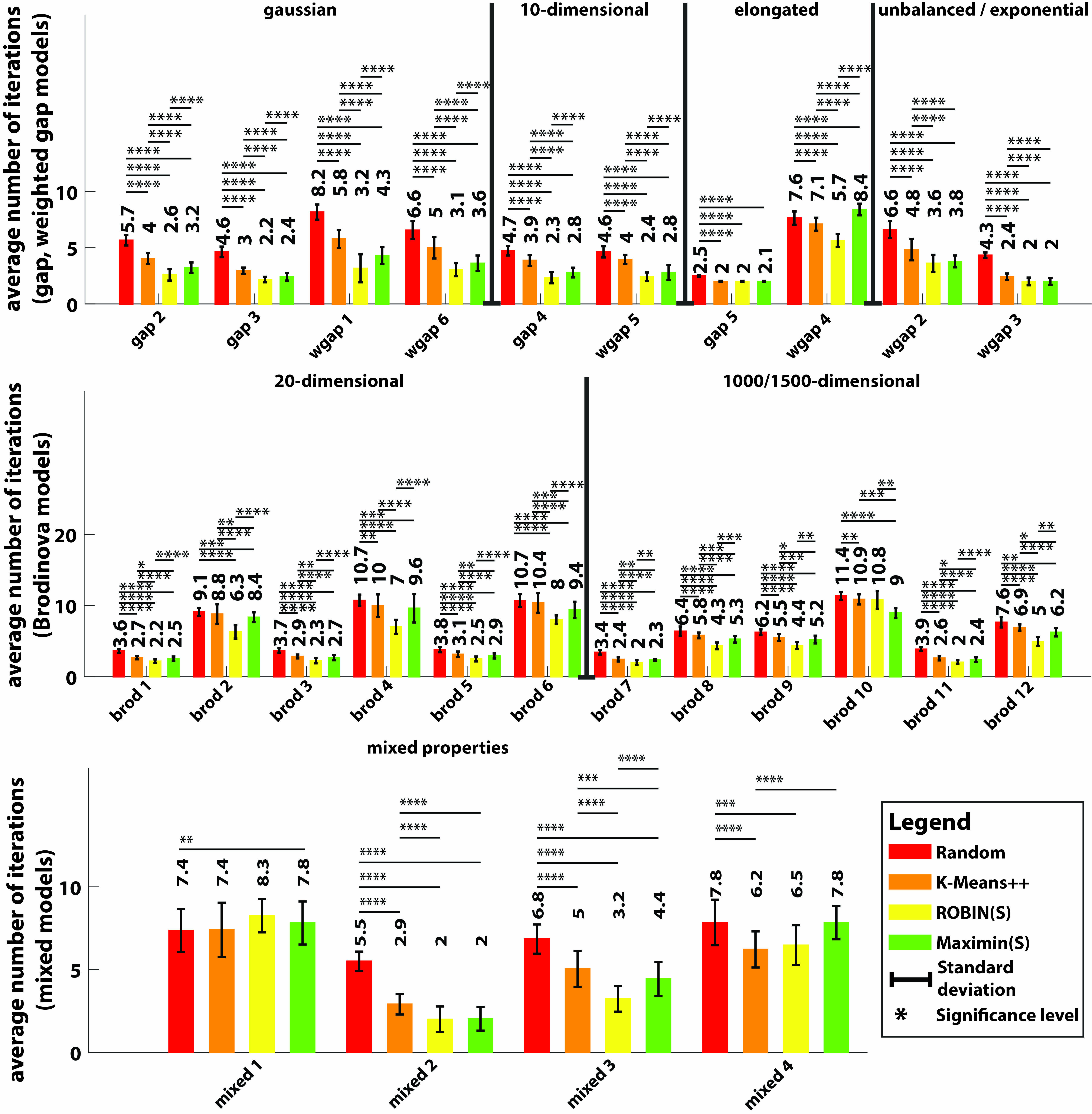
Figure 1: Average number of iterations until convergence for the stochastic methods. Each plot shows the number of iteration of the Lloyd’s K-Means algorithm (y-axis) until it reaches convergence using different stochastic initialisation methods on different data sets models (x-axis). To calculate the average number of iterations, we averaged the number of iterations across the 25 runs on the 40 data sets for each model (gap, weighted gap, Brodinova and mixed). The standard deviation corresponds to the average standard deviation over the 25 runs of each data set. Solid lines on any two bars underline the level of significant difference between the corresponding methods (cases of no significant differences are not showing). Table 5 shows a summary of the comparisons among all the different initialisation methods.

In our experiments we use the synthetic data from the studies of Tibshirani et al. (gap statistic) [35], Yan and Ye (weighted gap statistic) [36] and Brodinova et al. [12]. A summary of the models can be found in Table 1 grouped by specific properties of the models. For more information refer to the relevant studies and also to Figure 1 for a sample visualization of each model. We exclude model 1 from the gap statistic study [35] since it contains only one cluster. The Brodinova et al. [12] generator was used to generate high-dimensional data sets consisting of informative and non-informative features. No noise injection (attributes with noise contamination) was considered in the current study. To avoid situations of overlapping clusters the minimum Euclidean distance between any two points in different clusters was set to 3 and data sets violating this rule were re-generated. A summary of the models can be found in Table 2. Next we use our own synthetic data sets models consisted of clusters with mixed properties. We will refer to these models as mixed (refer to Figure 1 for a sample visualization of these models).

Table 1: Gap [35] and weighted gap statistic [36] data sets models. Points: the number of data points per cluster, or indicates that a random number was selected among the specified numbers for each cluster, to indicates that a random number was selected between the specified numbers for each cluster; p: number of features or attributes of the data set (dimensions); K: number of generated clusters. Gaussian models: clusters of low dimensionality generated from Gaussian distributions. 10-D Gaussian models: clusters of higher dimensionality generated from Gaussian distributions. Elongated models: clusters generated by adding Gaussian noise across lines. Unbalanced model: data sets containing Gaussian clusters of very different sizes, exponential: non-Gaussain clusters generated from the exponential distribution. For more information about the parameters used for the Gaussians refer to the relevant studies and the supplementary material. Visualization (when possible) of a data set from each model is available in Figure 1.

Gaussian models	Points	p	K		Unbalanced model	Points	p	K
gap model (gap 2)	25,25,50	2	3		weighted gap model 2 (wgap 2)	100,15	2	2
gap model 3 (gap 3)	25 or 50	3	4
weighted gap model 1 (wgap 1)	25 to 50	2	6		Exponential model	Points	p	K
weighted gap model 6 (wgap 6)	50 each	2	6		weighted gap model 3 (wgap 3)	50 each	2	4
10-D Gaussian models	Points	p	K		Elongated models	Points	p	K
gap model 4 (gap 4)	25 or 50	10	2		gap model 5 (gap 5)	100 each	3	2
weighted gap model 5 (wgap 5)	25 to 50	10	2		weighted gap model 4 (wgap 4)	100 each	2	2

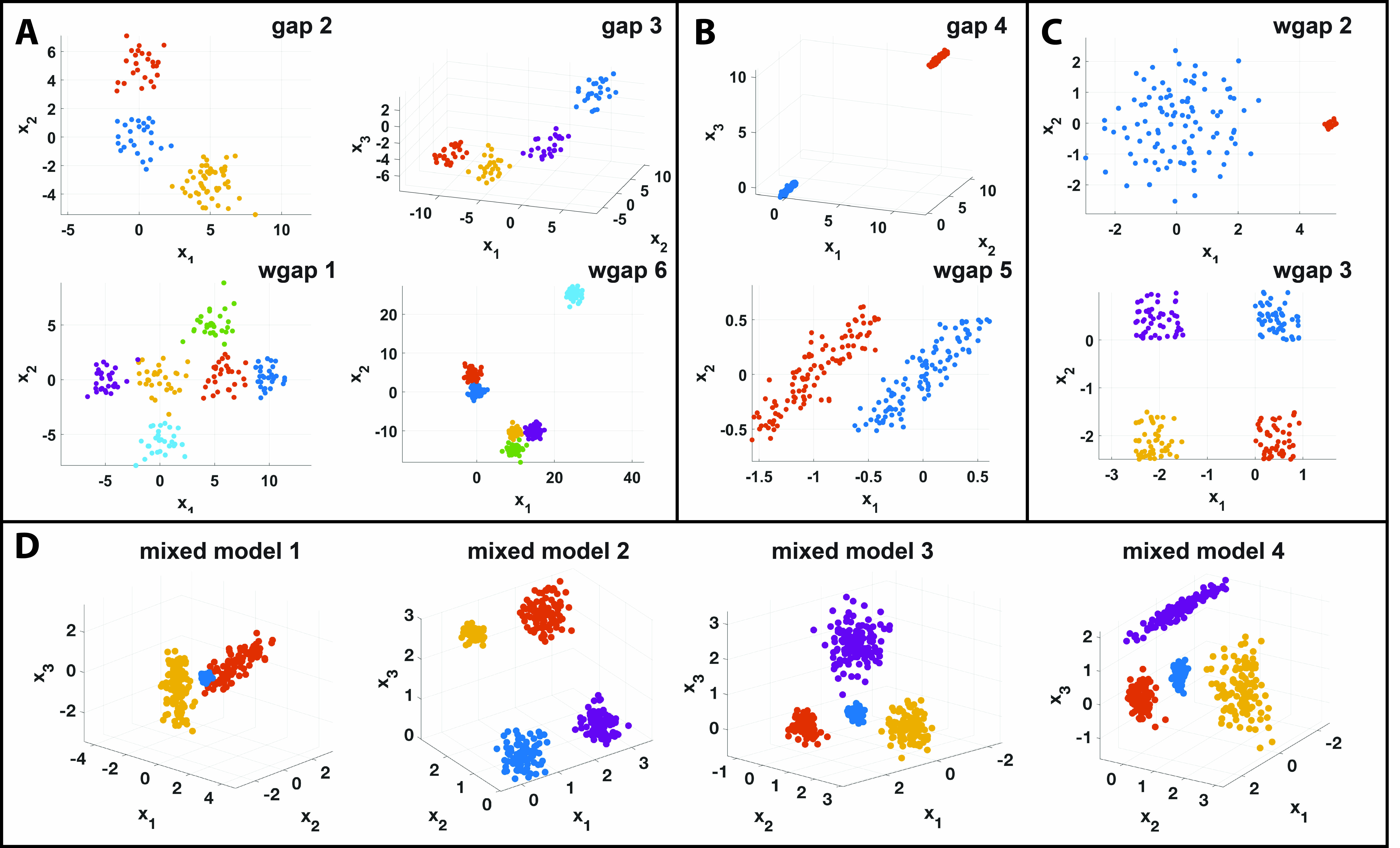
Figure 1: Model visualization. Examples of data used in this study. Gap (gap) and weighted gap (wgap) models are separated into three categories: (A) 4 Gaussian models, (B) 2 elongated models and (C) one highly unbalanced model (wgap2) and one non-Gaussian model (wgap3) in which the clusters are generated from the exponential distribution. (D) Mixed models: these are the additional models proposed in our study that contain clusters with mixed properties such as different sizes (unbalanced) and/or generated from Gaussian and non-Gaussian distributions.

Table 2: Brodinova model generator [12]. The minimum allowed Euclidean distance between two data points in different clusters was set to 3 and no noise injection was considered. Name: name of the model; Points: the total number of data points in the data set; p: number of features or attributes of the data set, Informative (+) indicates attributes that are required to describe the data set while Non-informative (-) indicates variables that should be ignored; K: number of generated clusters. These models are creating high-dimensional Gaussian clusters of different shapes using two different distributions, one for the informative and one for the uninformative variables. Left table: Each cluster contains 40 data points. The parameters of these models are selected to test the performance of the clustering algorithm in data sets with different degrees of informative and/or uninformative features Right table: The first four models create higher-dimensional balanced clusters (clusters of equal sizes) and the last two higher-dimensional unbalanced clusters each with number of points randomly selected between 50 to 100. The parameters of these models are selected to test the performance of the clustering algorithm in balanced and unbalanced data sets of higher dimensionality with increasing number of clusters. The input space was selected to be sparse, i.e. a few hundred points in 1000 or 1500 dimensions to avoid the slow computation of the Kaufman algorithm.

Name	Points	p		K
		+	-
brod 1	xx120xx	x20x	0	3
brod 2	400	20	0	10
brod 3	120	15	5	3
brod 4	400	15	5	10
brod 5	120	10	10	3
brod 6	400	10	10	10

Name	Points	p		K
		+	-
brod 7	120	1000	0	3
brod 8	400	1000	0	10
brod 9	400	1500	0	10
brod 10	1250	1500	0	50
brod 11	50 to 100	1000	0	3
brod 12	50 to 100	1000	0	10

• model 1 generates 3-dimensional clusters, 1 spherical and 2 elongated. The spherical cluster is an 80 points Gaussian cluster at the origin with standard deviation of 0.1. The two elongated clusters have 100 points each and are generated as follows: $x_{1}=x_{2}=x_{3}=t$ with $t$ taking 100 equally spaced values from -1 to 1. We then add Gaussian noise with standard deviation of 0.3 to each dimension. The second dimension of the first elongated cluster was shifted by 2 from the centre of the spherical cluster. Similarly the second dimension of the second elongated cluster was shifted by -2 and the first dimension was rotated by $180^{0}$.

• model 2 generates 3-dimensional non-Gaussian and normal clusters. It generates: (a) a cluster from an exponential distribution with rate of 1 and truncated at $[-1\hphantom{x}1]$ containing 80 points, (b) a cluster from an exponential distribution with rate of 1 and and truncated at $[2\hphantom{x}3]$ with 100 points, (c) a Gaussian cluster of 80 points with mean $[0.5,2.5,2.5]$ and standard deviation of 0.1 in every dimension and (d) a Gaussian cluster of 100 points with mean $[2.5,0.5,0.5]$ and standard deviation of 0.2 in every dimension.

• model 3 generates 3-dimensional Gaussian clusters with different standard deviations. The first cluster has 80 points with mean at the origin and standard deviation of 0.1 on each dimension. The second cluster has of 100 points with mean $[2,0,0]$ and standard deviation of 0.2 on each dimension. The third cluster has of 120 points with mean $[0,2,0]$ and standard deviation of 0.3 on each dimension. The forth cluster consists of 140 points with mean $[0,0,2]$ and standard deviation of 0.4 on each dimension.

• model 4 generates 3-dimensional mixed Gaussian clusters. The first cluster consists of 80 points with mean $[0,0,0]$ and standard deviations $[0.1,0.1,0.2]$. The second cluster consists of 100 points with mean $[2,0,0]$ and standard deviations $[0.1,0.2,0.3]$. The third cluster consists of 120 points with mean $[0,2,0]$ and standard deviations $[0.2,0.4,0.6]$. The forth cluster consists of 140 points with mean $[0,0,2]$ and standard deviations $[1.0,0.1,0.1]$.

We also consider the S-sets [37] and the A-sets [38] obtained from the “clustering basic benchmark” which was used in the studies of [20, 13]. The aforementioned studies were dedicated to the K-Means properties, advantages and disadvantages and assessed used various synthetic data sets. Both models contains 2-dimensional data; S-sets contains 4 data sets with 5000 data points distributed among 15 Gaussian clusters with different degree of clustering overlap [37] and A-sets contains 3 data sets with 20, 35 and 50 clusters and 150 data points per cluster [38]. For more information about these data sets refer to the relevant studies. Finally we considered a selection of data sets from the UCI repository [39]: Iris, Ionosphere, Wine, Breast Cancer, Glass and Yeast. More information about these data sets are shown on Table 3.

Table 3: Real data sets from the UCI repository [39]. Points: the number of data points per cluster; p: number of features or attributes of the data set (dimensions); K: number of generated clusters.

Name	Points	p	K
Iris	50,50,50	4	3
Ionosphere	225,126	34	2
Wine	59,71,48	13	3
Breast Cancer	444,239	9	2
Glass	70,76,17, 19,9,29	9	6
Yeast	463,5,35,44, 51,163,244, 429,20,30	8	10

4 Results

We test the performance of the K-Means variations, Lloyd’s [2] Hartigan-Wong’s [19, 4] and K-Medians [5] initialised using the eight different clustering initialisation methods named: Random [14], K-Means++ [15], Maximin(S) [16], ROBIN(S) [12], Kaufman [17], ROBIN(D) [11], DK-Means++ [18] and Maximin(D) [28]. For the ROBIN variations the $mp$ parameter specifying the number of neighbor data points was set to $10$ as in the original study [11]. For the Hartigan-Wong’s algorithm NAG’s implementation was used [40].

We conceptually consider a “sophistication” scale for the initialisation methods based not only on their execution time but also on the complexity of their underlying operators. For example DK-Means++ and ROBIN would be considered more sophisticated than Kaufman since they incorporate more advanced statistics while Kaufman uses only distances and still has a complexity of $O(N^{2})$. Our scale is as follows: Random $<$ K-Means++ $<$ Maximin $<$ Kaufman $<$ ROBIN $<$ DK-Means++.

In our experiments we use the synthetic data sets models from the studies of gap statistic [35] and weighted gap statistic [36] (refer to Table 1, 10 sets in total), Brodinova [12] (refer to Table 2, 12 sets in total) and other four custom data sets models (refer to Methods and Figure 1, 4 sets in total). From each model we generated 40 data sets and for each data set the stochastic methods were executed 50 times. These numbers were selected to provide a good statistical sample. We also use the “clustering data sets” (S-sets [37] and A-sets [38]) from the studies of [20, 13] and real-world data sets from the UCI repository [39]: Iris, Ionosphere, Wine, Breast Cancer, Glass and Yeast (see Table 3). For each of these data sets we use the same set up of executing the stochastic methods 50 times.

For all our hypothesis testing on the data set models we used the Paired Samples Wilcoxon Test, a non-parametric alternative to paired t-test, For the outcome of the test we generally use the following symbols for the level of significance, $*$ for p-value $<$ 0.05; $**$ for p-value $<$ 0.01; $***$ for p-value $<$ 0.001; $****$ for p-value $<$ 0.0001. We evaluated the monotonic relationship of Silhouette index and Purity via a large sample of clustering results on the multiple executions of the methods across all our data sets (20000 cases). Using Spearman’s rank correlation coefficient, we confirmed that Purity and Silhouette have a strong monotonic relation (Spearman’s Rho $0.97$). As a side note, we also considered Distortion [11] as an unsupervised index but found the monotonic relationship with Purity weaker (Spearman’s Rho $0.65$).

Table 4: Average performance comparison among K-Means variations using simple stochastic and more sophisticated deterministic initialisation methods. We compare two K-Means variations (Hartigan-Wong’s K-Means: HW, Lloyd’s K-Means: Ll and K-Medians: KMed) initialised with the same method on 26 occasions (10 gap and weighted gap, 12 Brodinova and 4 mixed models). To calculate performance, we averaged the Purity index across the 50 initial conditions and 40 data sets for each model and the comparison is based on the times that there was significant difference between the two algorithms.

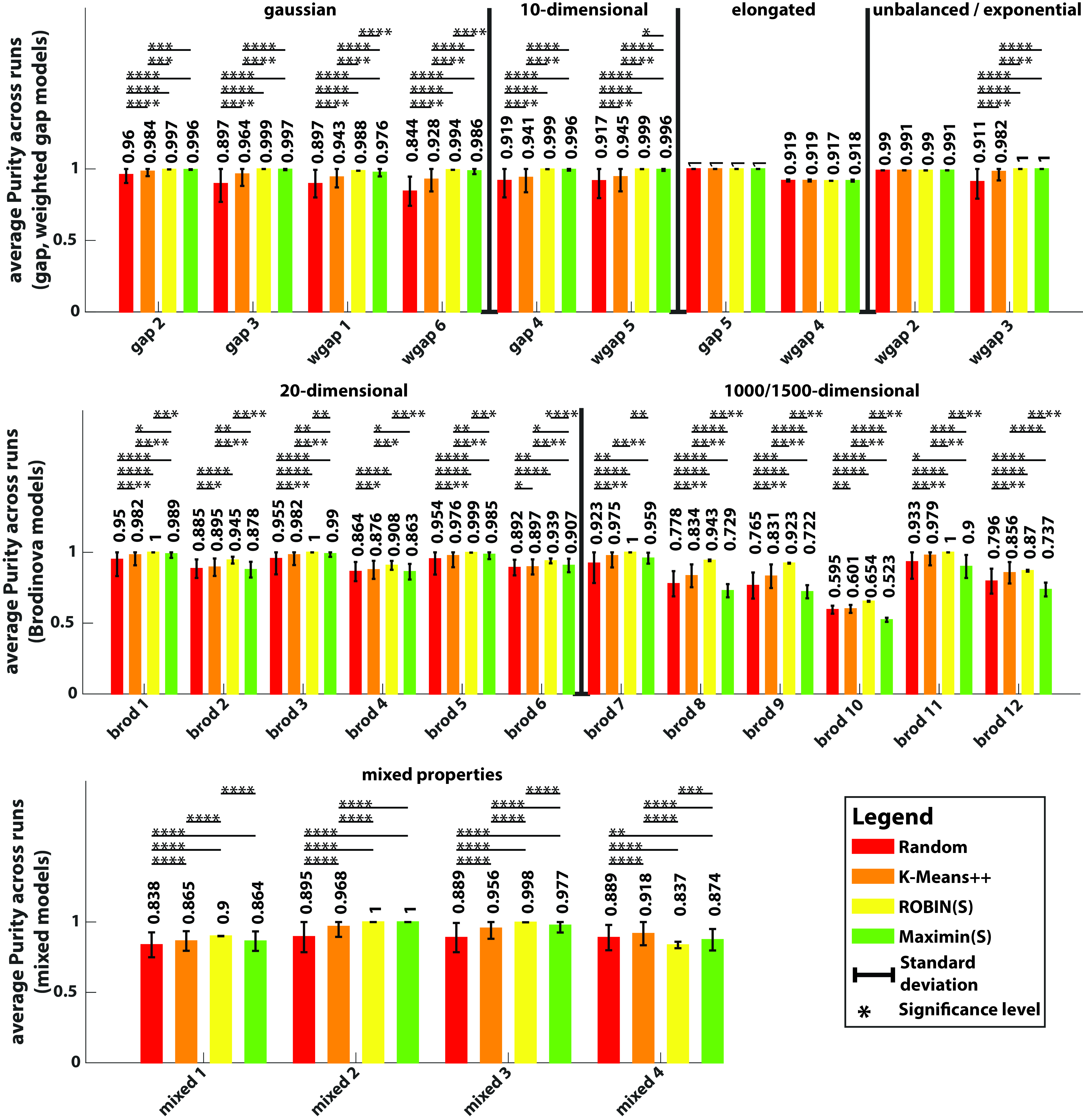
		Significantly better average performance
Initialization method	Total number of instances	HW vs Ll	HW vs KMed	Ll vs KMed
Random	26	13 vs 0	18 vs 4	6 vs 4
K-Means++	26	10 vs 0	13 vs 3	2 vs 5
Total	52	23 vs 0	39 vs 12	8 vs 9
Kaufman	26	1 vs 1	2 vs 6	1 vs 6
DK-Means++	26	1 vs 0	2 vs 4	1 vs 5
Total	52	2 vs 1	4 vs 10	2 vs 11

4.1 Comparison on the average performance among stochastic and among deterministic methods

We assess on average the performance of stochastic methods as well as the performance of deterministic methods. We calculate the average performance of stochastic methods on 50 different runs across 40 different data sets for each one of our 26 models (10 gap and weighted gap, 12 Brodinova, 4 mixed models). Deterministic methods were executed once on the 40 data sets.

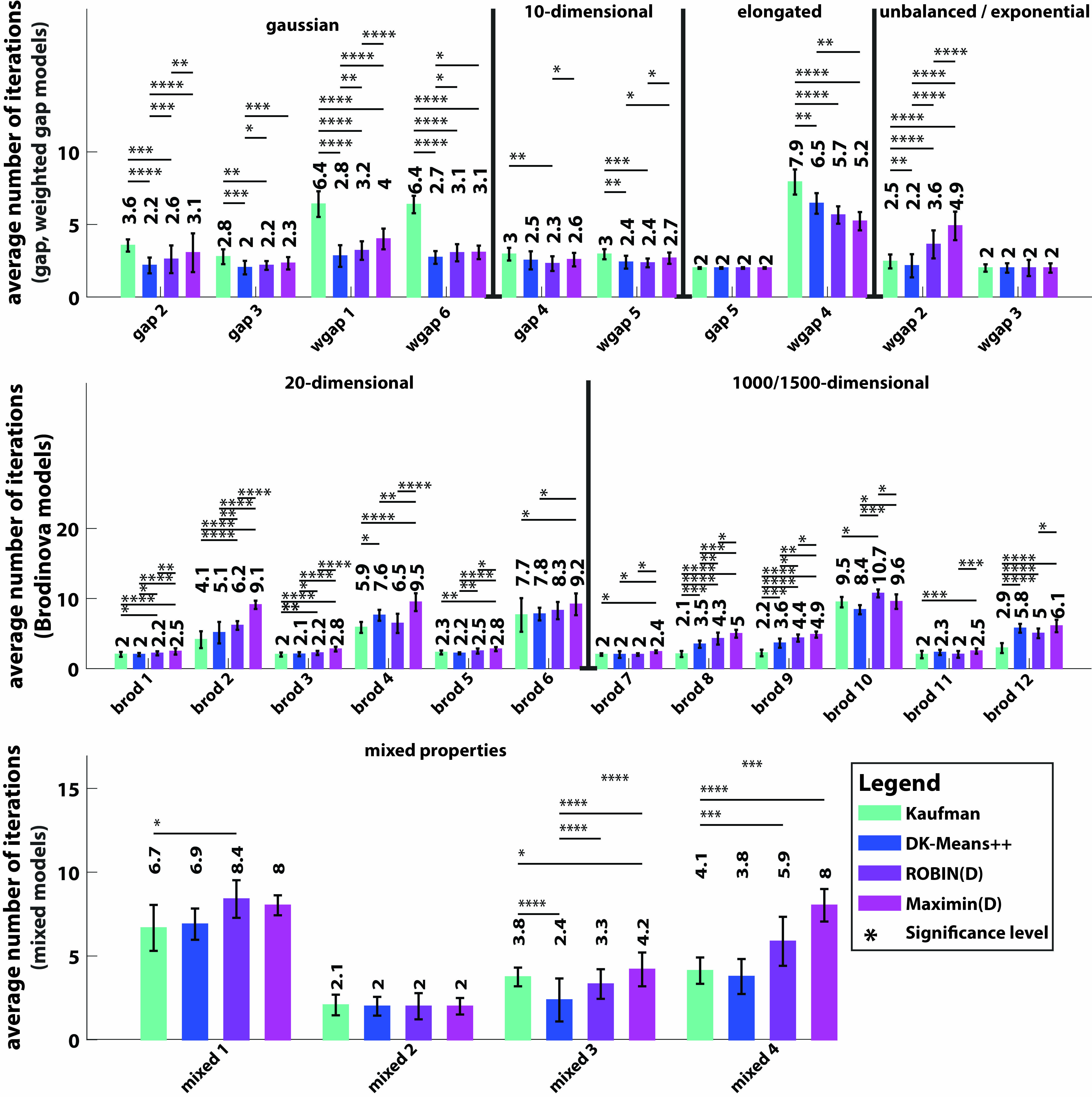
Figure 2: Average number of iterations until convergence for the stochastic methods. Each plot shows the number of iteration of the Lloyd’s K-Means algorithm (y-axis) until it reaches convergence using different deterministic initialisation methods on different data sets models (x-axis). To calculate the average number of iterations, we averaged the number of iterations across the 25 runs on the 40 data sets for each model (gap, weighted gap, Brodinova and mixed). The standard deviation corresponds to the average standard deviation over the 25 runs of each data set. Solid lines on any two bars underline the level of significant difference between the corresponding methods (cases of no significant differences are not showing). Table 5 shows a summary of the comparisons among all the different initialisation methods.

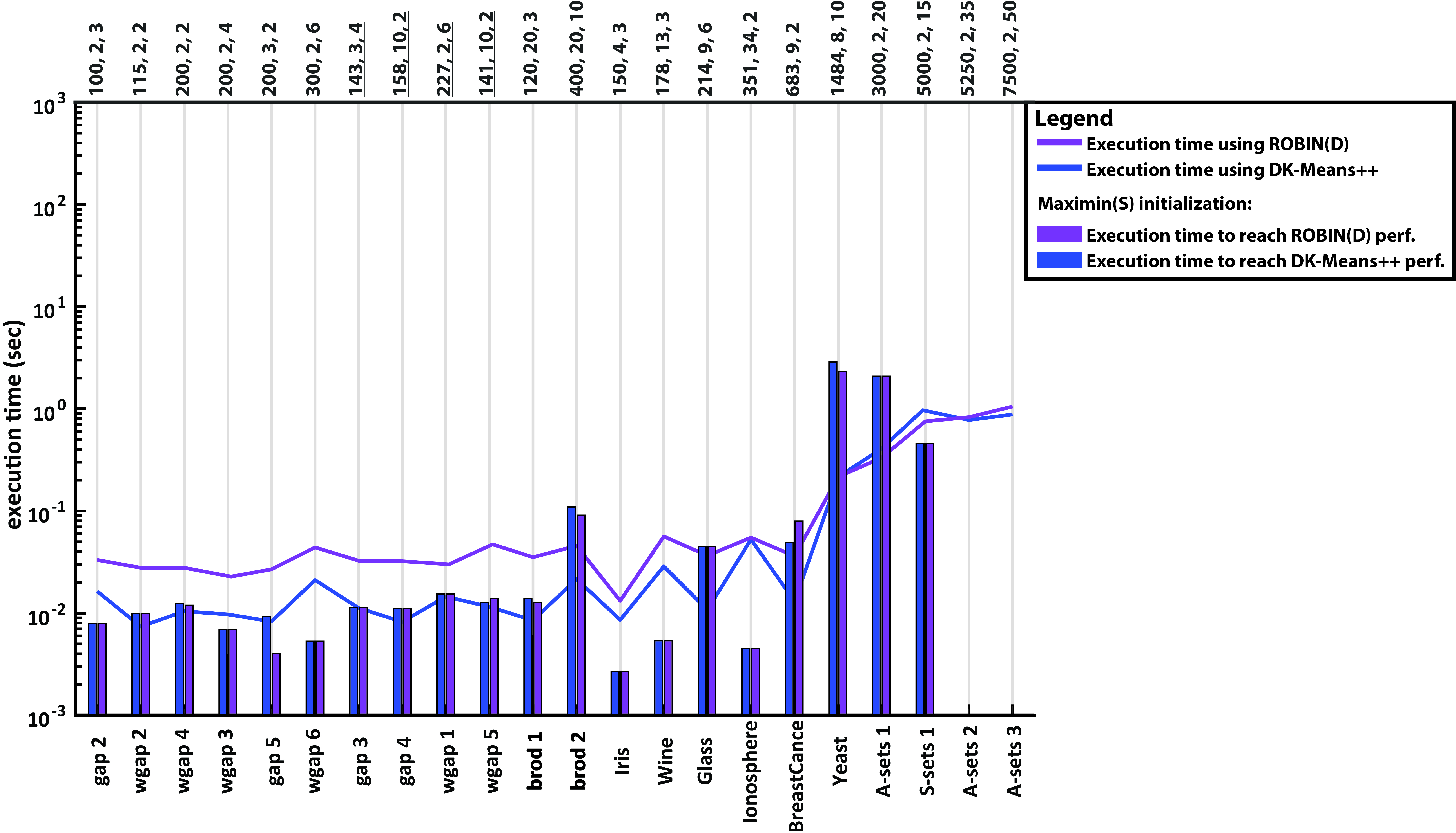
Figure 3: Execution time analysis for K-Means clustering with Maximin(S) initialisation to reach the performance of DK-Means++ and ROBIN(D). Each bar shows the execution duration of K-Means clustering algorithm executed multiple times with the Maximin(S) initialisation method until reaching the performance of the clustering algorithm running once using DK-Means++ and ROBIN(D) methods. Lines indicate the execution time of K-Means clustering running once using the deterministic methods ROBIN(D) and DK-Means++. The clustering algorithm was given 50 execution repetitions with the stochastic Maximin(S) method to reach an equal or better solution than deterministic methods. Data sets without a bar means that no equal or better solution compared to the respective clustering with a deterministic method was found. The data sets are arranged based on their size, dimensionality and number of clusters (see info on top, underlined numbers means that for these models the generated data sets had different sizes). Results were averaged over 40 data sets for the data set models.

Based on Figure 2 the average performance of K-Means variations increases by using more sophisticated initialisation methods and ROBIN(S) initialisation provides the best average performance followed by Maximin(S) and K-Means++ while Random initialisation results in the poorest performance. For the deterministic methods, shown on Figure 3, we observe again that the average performance of K-Means variations increases by using more sophisticated initialisation methods. DK-Means++ achieved the best average performance followed by ROBIN(D) and then by Kaufman and Maximin(D). Finally we wanted to assess if more sophisticated initialization methods alleviate the need for complex clustering. For this reason we performed comparisons among the K-Means variations initialised with either Random and K-Means++ or Kaufman and DK-Means++ methods. Maximin and ROBIN have both stochastic and deterministic variations of equal sophistication thus we excluded them. As shown in Table 4, deterministic methods that are more sophisticated (as per our definition) reduce performance differences among the different variants of the K-Means algorithms.

		Significantly better average performance
Initialization method	Total number of instances	HW	Ll	KMed
Random vs K-Means++	26	0 vs 23	0 vs 23	0 vs 24
Random vs ROBIN(S)	26	1 vs 22	3 vs 22	2 vs 23
Random vs Maximin(S)	26	6 vs 15	6 vs 16	6 vs 16
K-Means++ vs ROBIN(S)	26	1 vs 21	3 vs 21	2 vs 22
K-Means++ vs Maximin(S)	26	8 vs 13	9 vs 14	7 vs 13
ROBIN(S) vs Maximin(S)	26	17 vs 1	18 vs 3	19 vs 1

Figure 2: Comparison on the average performance among stochastic initialisation methods. Each plot shows the performance of the Hartigan-Wong’s K-Means clustering solution using the Purity index (y-axis) on different data sets models (x-axis) and initialized with different stochastic methods. To calculate performance, we averaged the Purity index across the 50 initial conditions and 40 data sets for each model (gap, weighted gap, Brodinova and mixed). The errorbars are showing the (average) standard deviation across the 40 data sets. Solid lines on any two bars underline the level of significant difference between the corresponding methods. The accompanied Table below the figure shows a summary of the comparisons through all the K-Means variations (Hartigan-Wong’s K-Means (HW), Lloyd’s K-Means (Ll) and K-Medians (KMed)) where there is a significant performance difference between the compared methods.

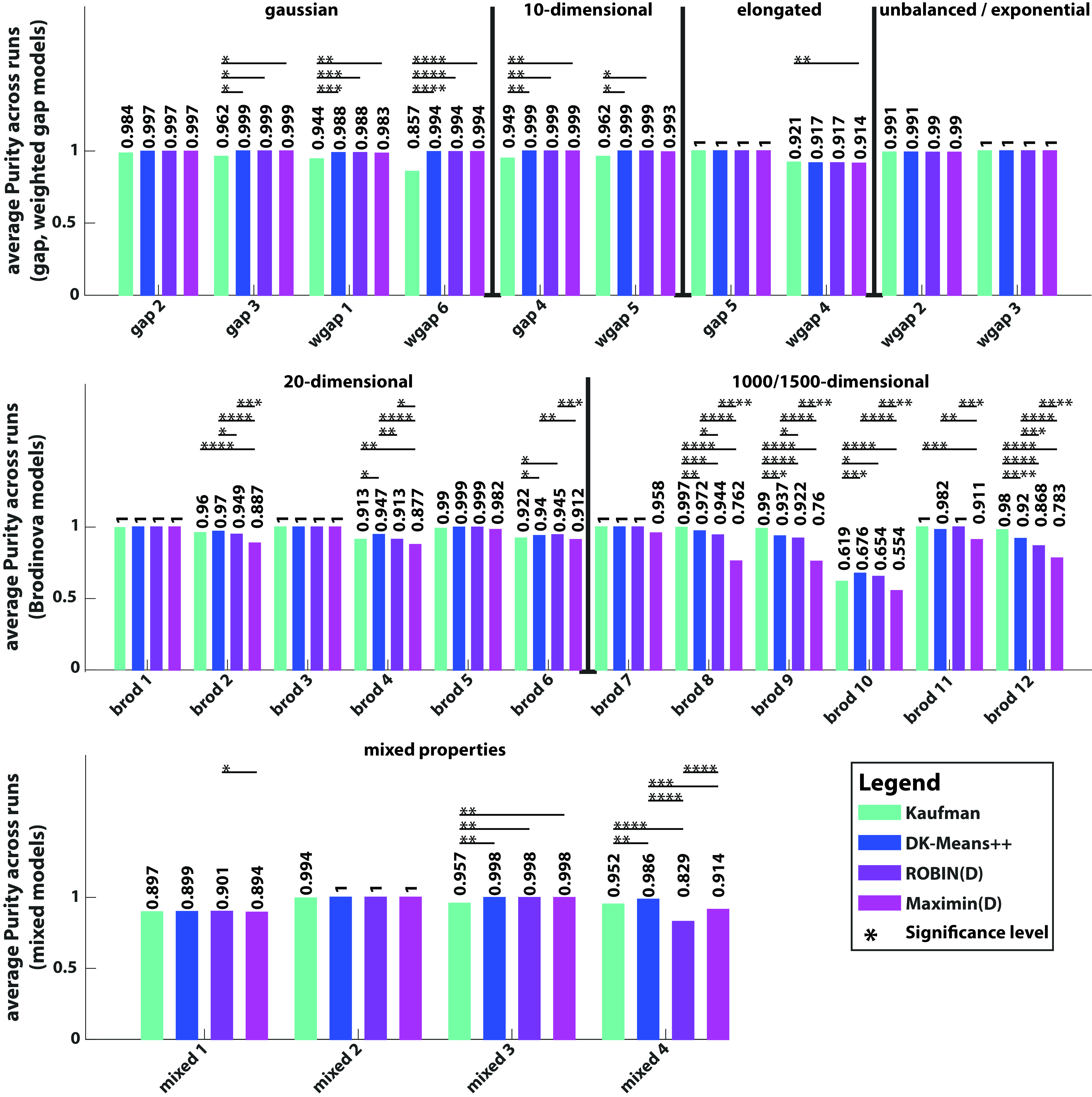
		Significantly better average performance
Initialization method	Total number of instances	HW	Ll	KMed
Kaufman vs DK-Means++	26	3 vs 10	3 vs 9	4 vs 8
Kaufman vs ROBIN(D)	26	4 vs 8	6 vs 9	4 vs 6
Kaufman vs Maximin(D)	26	8 vs 5	11 vs 5	9 vs 5
DK-Means++ vs ROBIN(D)	26	6 vs 0	7 vs 0	6 vs 1
DK-Means++ vs Maximin(D)	26	9 vs 0	11 vs 0	10 vs 1
ROBIN(D) vs Maximin(D)	26	9 vs 1	10 vs 1	9 vs 1

Figure 3: Comparison on the performance among deterministic initialisation methods. Each plot shows the performance of the Hartigan-Wong’s K-Means clustering solution using the Purity index (y-axis) on different data sets models (x-axis) and initialized with different deterministic methods. To calculate performance, we averaged the Purity index across the 40 data sets for each model (gap, weighted gap, Brodinova and mixed). Solid lines on any two bars underline the level of significant difference between the corresponding methods (cases of no significant differences are not showing). The accompanied Table below the figure shows a summary of the comparisons through all the K-Means variations (Hartigan-Wong’s K-Means (HW), Lloyd’s K-Means (Ll) and K-Medians (KMed)) where there is a significant performance difference between the compared methods.

4.2 Comparison of the average performance between stochastic and deterministic methods

Following on from our previous conclusions, we wanted to assess if overall deterministic methods provide on average better performance than stochastic methods. For this reason we compared the stochastic and deterministic variations of Maximin and ROBIN as well as the best stochastic performer (ROBIN(S) see Figure 2) and the best deterministic performer (DK-Means++ see Figure 3). Based on the results in Figure 4: (a) Maximin(D) is on average better than Maximin(S); (b) ROBIN(D) and ROBIN(S) are on average equivalent; (c) DK-Means++ is better than ROBIN(S).

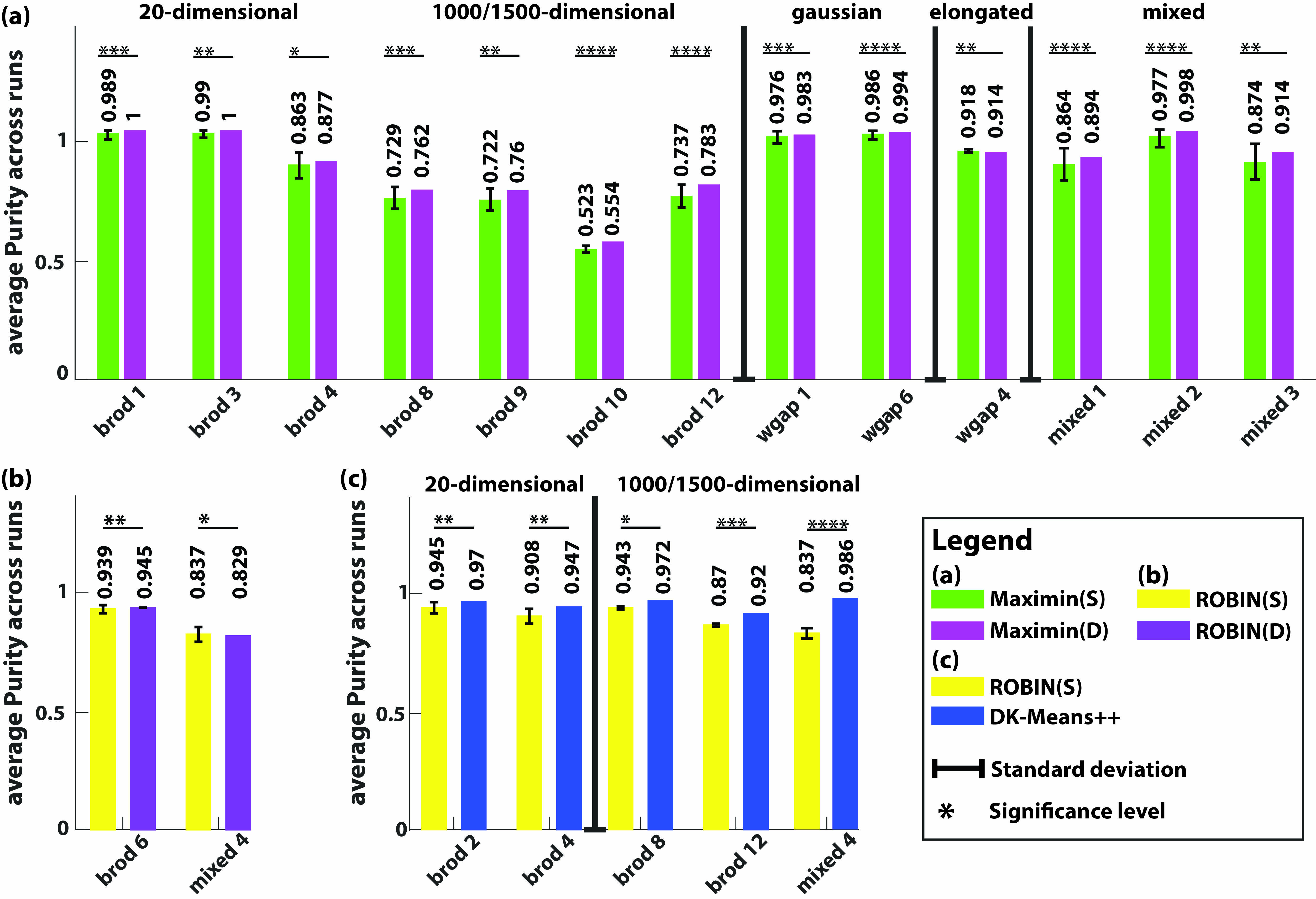
Initialization method	Total number of instances	Significantly better average performance
		HW	Ll	KMed
Maximin(S) vs Maximin(D)	26	1 vs 12	3 vs 12	0 vs 13
ROBIN(S) vs ROBIN(D)	26	1 vs 1	1 vs 2	1 vs 0
ROBIN(S) vs DK-Means++	26	0 vs 5	0 vs 7	1 vs 5

Figure 4: Comparisons on the average performance between stochastic and deterministic methods. Each plot shows the performance of the Hartigan-Wong’s K-Means clustering solution using the Purity index (y-axis) on different data sets models (x-axis) and initialized with different stochastic methods (only the cases where significant difference was present are shown). To calculate performance, we averaged the Purity index across the 50 initial conditions and 40 data sets for each model (gap, weighted gap and Brodinova). The errorbars (on the stochastic methods only) are showing the average standard deviation across the 40 data sets. Solid lines on any two bars underline the level of significant difference between the corresponding methods (cases of no significant differences are not showing). The accompanied Table below the figure shows a summary of the comparisons through all the K-Means variations (Hartigan-Wong’s K-Means (HW), Lloyd’s K-Means (Ll) and K-Medians (KMed)) where there is a significant performance difference between the compared methods.

4.3 Comparison of the maximum performance across multiple runs of stochastic and deterministic methods

Next, we wanted to compare the stochastic and the deterministic methods but based on the maximum performance that the former can achieve on multiple repetitions. We run each of the stochastic methods 50 times and select the best outcome based on the silhouette index. We then report its corresponding value according to the purity index. We expect that due to the many repetitions, stochastic methods can find different local minima and potentially result in a better performance at the cost of multiple repetitions.

Firstly, we repeat the comparison among the different stochastic methods but based on the maximum performance that they can achieve. Figure 5 shows the relevant results and, opposite to our observations on the average performance, stochastic methods have higher chances of obtaining a better clustering result with multiple execution. K-Means++ is the best method followed by Random while ROBIN(S) and Maximin(S) have almost similar performance.

Afterwards, we compared the maximum performance of stochastic methods with the performance of deterministic methods similarly to our previous experiment (refer to Figure 4). We compare the stochastic and deterministic variations of Maximin and ROBIN as well as the best stochastic performer of the current experiment (K-Means++) and the best deterministic performer (DK-Means++ see Figure 3). Based on the results in Figure 6, stochastic variations of Maximin and ROBIN achieve overall better performance than their deterministic counterparts and K-Means++ is better than DK-Means++.

We also compare the K-Means variations using different intialisation methods. Based on the result on Table 5 K-Medians achieves the best performance followed by Hartigan-Wong’s; Lloyd’s was the worst performer. Nevertheless, these systematic differences correspond to only $1.5\%$ purity difference.

Table 5: Best performance comparison on K-Means variations using different initialisation methods. Each row compares two K-Means variations (Hartigan-Wong’s K-Means: HW, Lloyd’s K-Means: Ll and K-Medians: KMed) initialised with the same method on 26 occasions (10 gap and weighted gap, 12 Brodinova and 4 mixed models). The comparison is based on the times that there was significant difference between the two methods on their maximum performance based on the purity for the best silhouette score.

		Significantly better maximum performance
Initialization method	Total number of instances	HW vs Ll	HW vs KMed	Ll vs KMed
Random	26	4 vs 1	3 vs 7	1 vs 7
K-Means++	26	5 vs 1	2 vs 7	1 vs 4
ROBIN(S)	26	4 vs 0	1 vs 3	1 vs 7
Maximin(S)	26	2 vs 1	3 vs 5	2 vs 3
Total	104	15 vs 3	9 vs 22	5 vs 21
Kaufman	26	1 vs 1	2 vs 6	1 vs 6
DK-Means++	26	1 vs 0	2 vs 4	1 vs 5
ROBIN(D)	26	6 vs 0	2 vs 2	1 vs 6
Maximin(D)	26	7 vs 0	2 vs 2	1 vs 6
Total	104	15 vs 1	8 vs 14	4 vs 23

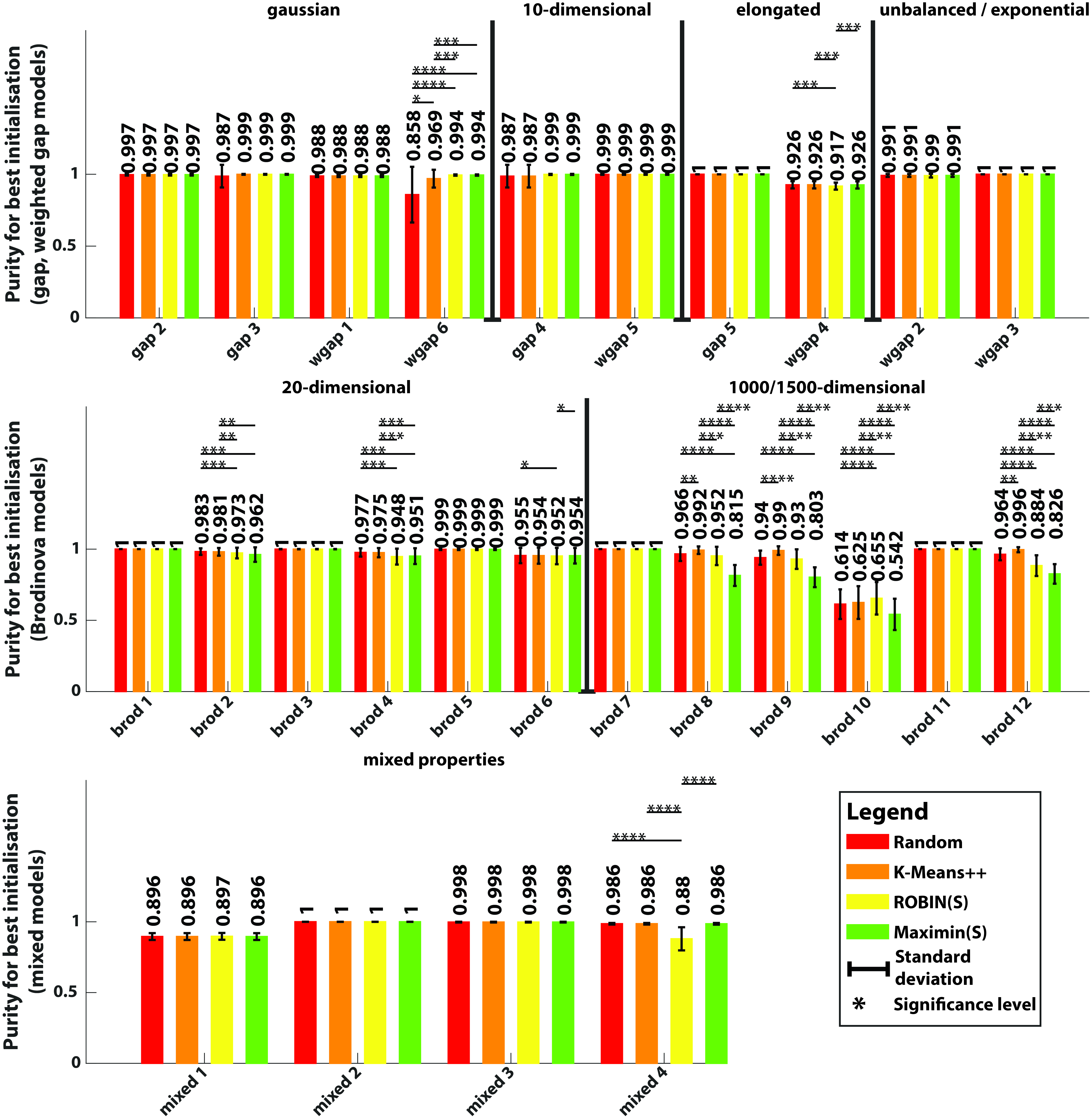
Initialization method	Total number of instances	Significantly better maximum performance Purity for best Silhouette
		HW	Ll	KMed
Random vs K-Means++	26	0 vs 4	0 vs 4	1 vs 4
Random vs ROBIN(S)	26	6 vs 3	8 vs 2	6 vs 2
Random vs Maximin(S)	26	6 vs 1	9 vs 1	9 vs 1
K-Means++ vs ROBIN(S)	26	7 vs 2	9 vs 2	8 vs 2
K-Means++ vs Maximin(S)	26	6 vs 1	9 vs 1	9 vs 1
ROBIN(S) vs Maximin(S)	26	4 vs 3	4 vs 4	4 vs 2

Figure 5: Comparison on the maximum performance among stochastic initialisation methods. Each plot shows the performance of the Hartigan-Wong’s K-Means clustering solution using the purity corresponding to the best silhouette score achieved within 50 different executions (y-axis) on different data sets models (x-axis) and initialized with different stochastic methods. Purity for best silhouette score was averaged over the 40 data sets for each model (gap, weighted gap and Brodinova) The errorbars are showing the standard deviation across the 40 data sets. Solid lines on any two bars underline the level of significant difference between the corresponding methods. The accompanied Table below the figure shows a summary of the comparisons through all the K-Means variations (Hartigan-Wong’s K-Means (HW), Lloyd’s K-Means (Ll) and K-Medians (KMed)) where there is a significant performance difference between the compared methods.

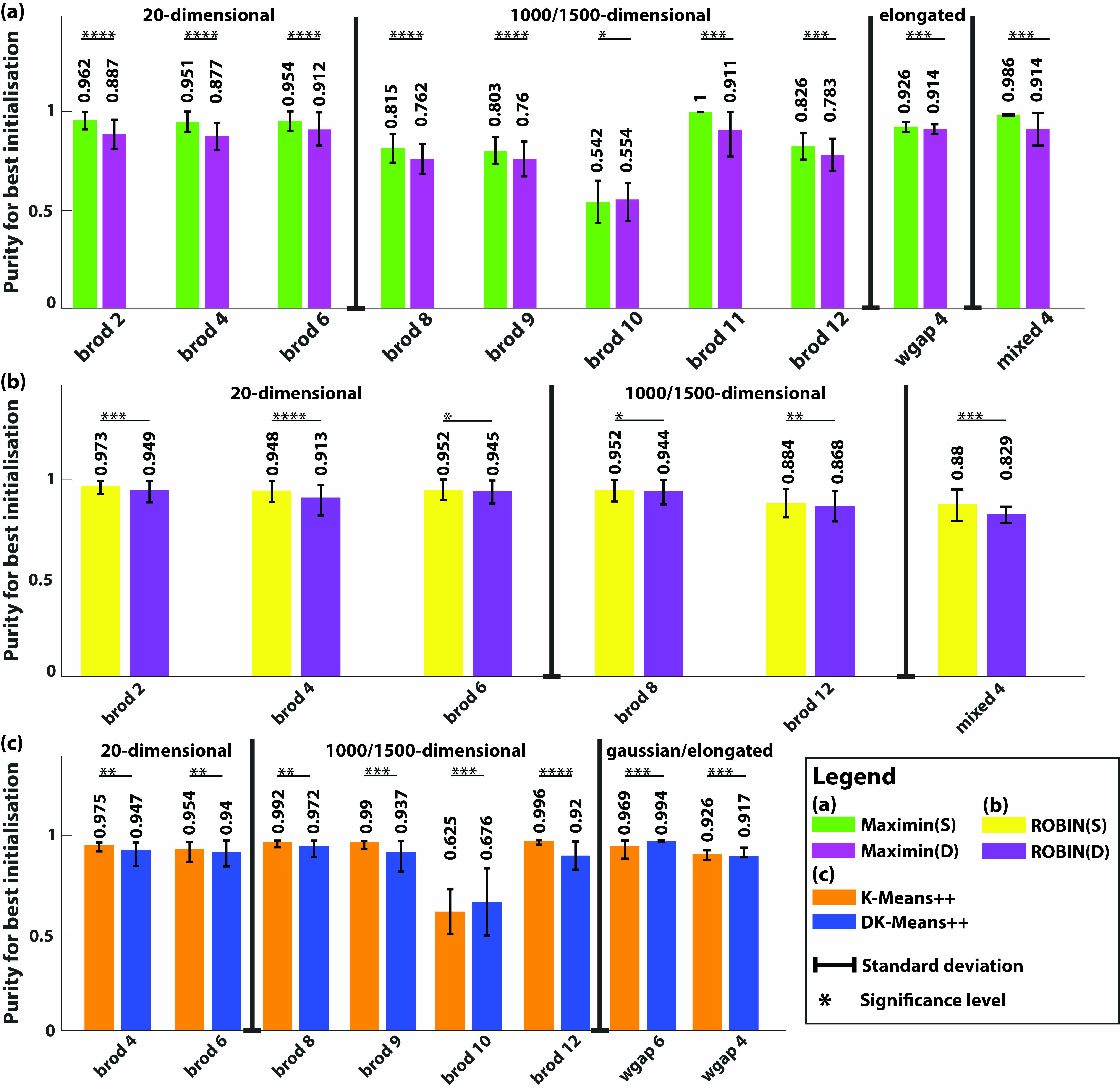
Initialization method	Total number of instances	Significant better average performance
		HW	Ll	KMed
Maximin(S) vs Maximin(D)	26	9 vs 1	11 vs 1	10 vs 1
ROBIN(S) vs ROBIN(D)	26	6 vs 0	6 vs 0	6 vs 0
K-Means++ vs DK-Means++	26	6 vs 2	6 vs 2	7 vs 2

Figure 6: Comparisons on the maximum performance between stochastic and deterministic methods. Each plot shows the performance of the Hartigan-Wong’s K-Means clustering solution using the purity corresponding to the best silhouette score achieved within 50 different executions (y-axis) on different data sets models (x-axis) and initialized with different stochastic methods (only the cases where significant difference was present are shown). Purity for best silhouette score was averaged over the 40 data sets for each model (gap, weighted gap and Brodinova). The errorbars are showing the standard deviation across the 40 data sets. Solid lines on any two bars underline the level of significant difference between the corresponding methods (only cases with significant difference are showed). The accompanied Table below the figure shows a summary of the comparisons through all the K-Means variations (Hartigan-Wong’s K-Means (HW), Lloyd’s K-Means (Ll) and K-Medians (KMed)) where there is a significant performance difference between the compared methods.

4.4 Standalone synthetic and real-world data sets

We regard the standalone data sets as cases where supervised information is unknown and we assess the performance of the algorithms based on the silhouette index. Detailed results for each data set (minimum, maximum, average performance and variance for each K-Means variation) are illustrated in the supplementary material. Given that these data sets are unique it is difficult to draw definite conclusions similar to the ones where data set models were used but we would like to highlight some observations. DK-Means++ was always able to achieve the best performance of the unsupervised methods while ROBIN(D) failed to achieve the best performance in the cases of A-sets 1, S-Sets 3 and S-Sets 4 when Lloyds and K-Medians were considered; Kaufman and Maximin(D) where the worst performers. From the stochastic methods ROBIN(S) always managed to achieve the maximum performance apart from one case of S-Sets 3 when the Harigan-Wong K-Means was considered; Random was the worst performer. For the real-world data sets most algorithms behaved the same but Maximin(S) outperformed everyone else in the cases of Yeast (all K-Means variations) and Ionosphere (Lloyd’s K-Means only). In the case of Glass (all K-Means variations) K-Means++ and Maximin(S) had the best performances. However, with the real data sets we should consider the fact that in rare situations the number of clusters equals to the number of classes [41] thus it might not be the best examples for clustering benchmarking. Also the relatively better performance of Maximin(S) appears only in these few cases where the Silhouette index indicates poor clustering results in general. In such cases comparative conclusions may not be meaningful as these specific results could be a product of chance.

4.5 Average number of runs for which stochastic methods reach or surpass deterministic methods

In the aforementioned experiments we considered 50 executions of the clustering algorithm using stochastic methods. On average deterministic methods provide better results than stochastic methods but overall stochastic methods may lead to a better clustering solution. We would therefore like to quantify how often this happens. To estimate this, we divide the number of total repetitions (50) by the number of cases where the stochastic method performed better than the deterministic. Table 6 summarises the results of this analysis on selected data sets based on their size, dimensionality and number of clusters among two stochastic (Random and K-Means++) and two deterministic methods (DK-Means++ and ROBIN(D)). Based on the results the number of repetitions required for the clustering method using K-Means++ in order to match or surpass the performance of DK-Means++ and ROBIN(D) are less compared with Random. This was expected given the performance comparison of Random and K-Means++ but an important result is the following: there are cases (Yeast, A-sets 2 and A-sets 3) where these stochastic methods fail to match or surpass the performance of deterministic methods under 50 runs. We also observe that when the size of the data set surpasses the 1000 data points the number of required repetitions is significantly high. Finally we should mention that these performance differences are minor, in the order of $10^{-3}$ (purity) on average.

	Rand DKM++	Rand ROBIN(D)	KM++ DKM++	KM++ ROBIN(D)	size, dimensions, number of clusters
gap 2	5	5	4	4	100,2,3
wgap 2	6	6	4	4	115,2,2
wgap 4	6	6	5	5	200,2,2
wgap 3	3	3	3	3	200,2,4
gap 5	4	2	4	2	200,3,2
wgap 6	8	8	7	6	300,2,6
gap 3	5	5	4	4	143,3,4
gap 4	10	10	6	6	158,10,2
wgap 1	7	7	6	6	227,2,6
wgap 5	14	14	6	6	141,10,2
brod 1	4	4	5	5	120,20,3
brod 2	18	17	17	17	400,20,3
Iris	7	7	3	3	150,4,3
Wine	3	3	2	2	178,13,3
Glass	7	7	6	6	214,9,6
Ionosphere	3	3	2	2	351,34,2
Breast Cancer	12	12	7	7	683,9,2
Yeast	N/A	16	27	14	1484,8,10
A-sets 1	28	26	26	16	3000,2,15
S-Sets 1	34	34	26	15	5000,2,15
A-sets 2	N/A	N/A	34	33	5250,2,35
A-sets 3	N/A	N/A	N/A	N/A	7500,2,50

Table 6: Average number of runs for which stochastic initialisations achieve equivalent or better performance than deterministic initialisations. Each column shows a comparison between clustering initialised with stochastic and deterministic methods (Rand = Random, DKM++ = DK-Means++, KM++ = K-Means++). Each cell value corresponds to the number of executions of the K-Means clustering initialised with the stochastic method to reach or surpass its performance if it was initialised with the deterministic method and executed once. N/A values mean that in these occasions the stochastic clustering was not able to match or surpass the performance of the deterministic clustering under $50$ executions. Values higher than $10$ are marked in bold. The data sets are arranged based on their size, dimensionality and number of clusters (see info on last column; numbers in italics correspond to the average number of elements should the model generated data sets of different sizes.

4.6 Execution time analysis

Finally, we performed an execution time analysis on the initialisation methods using a selection of the data sets depending on their size, dimensionality and number of clusters; data sets with equivalent properties were omitted. The analysis was performed as follows: each initialisation methods followed by K-Means clustering (Lloyd’s K-Means) was executed 50 times and the average running time was taken into consideration.

• The benchmarking was exclusively performed on a personal laptop with the following properties: Dell G7; Intel i7-9750H processor; 16 GB RAM; Windows 10 Pro edition.

• All the algorithms were written in MATLAB but the LOF score for ROBIN was computed using R code (specifically the dbscan package [42]) because we found that the MATLAB implementation was very slow.

• The running time recording includes the initialisation method and the clustering algorithm. For ROBIN the computation of LOF was included in the execution duration as well as the computation of $\varepsilon$ for the DK-Means++.

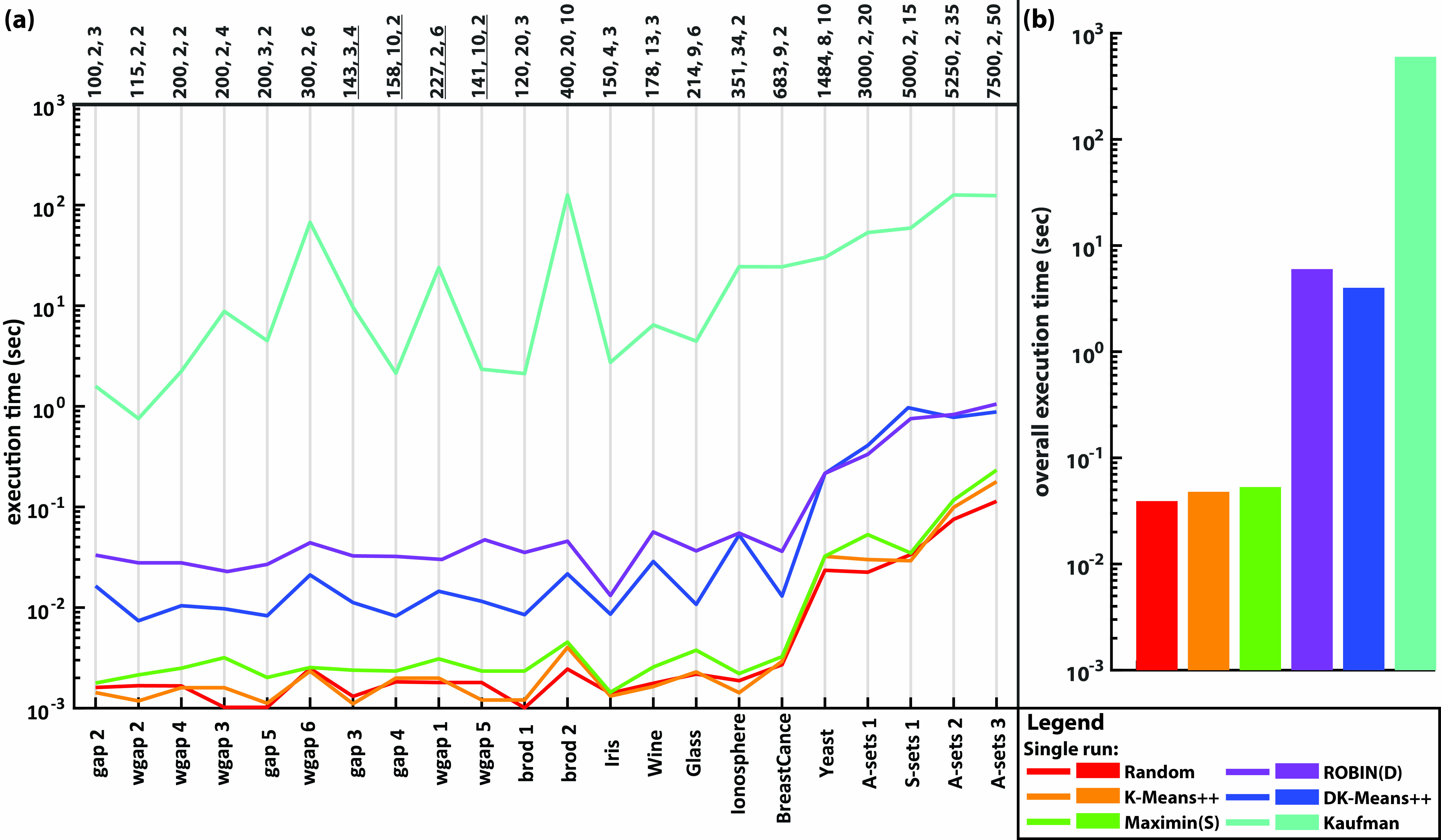
Figure 7: Execution time analysis. (a) Each line shows the execution duration of an initialisation method on different data sets selected based on size, dimensions and number of clusters. We average the execution time for 50 repetitions and, in case of models, across the 40 data sets of each model. The data sets are arranged based on their size, dimensionality and number of clusters (see info on top, underlined numbers means that for these models generate data sets of different sizes). (b) Each bar shows the summed execution time across all data sets of (a).

Based on the results in Figure 7 Kaufman is the worst method in terms of execution duration and it is affected both by the size, dimensionality and number of clusters. Random and K-Means++ are the fastest methods followed by Maximin(S). DK-Means++ is almost always better than ROBIN(D) in terms of speed for our implementation.

Furthermore, and based on the results of Table 6 we performed an analysis on the time requirements of the stochastic methods to reach or surpass the performance of deterministic methods with multiple executions of the clustering algorithm using different seeds. In Figure 8 we show the single run execution time of the stochastic initialisation (plus the clustering overhead) multiplied by the number of iterations required to surpass the deterministic methods (see Table 6). Based on the results shown in Figure 8 we observe that in many occasions running DK-Means++ once is better in terms of execution time than repeated runs of the clustering with a stochastic method. Equivalent conclusions can also be obtained from the Maximin(S) initialisation method (supplementary material).

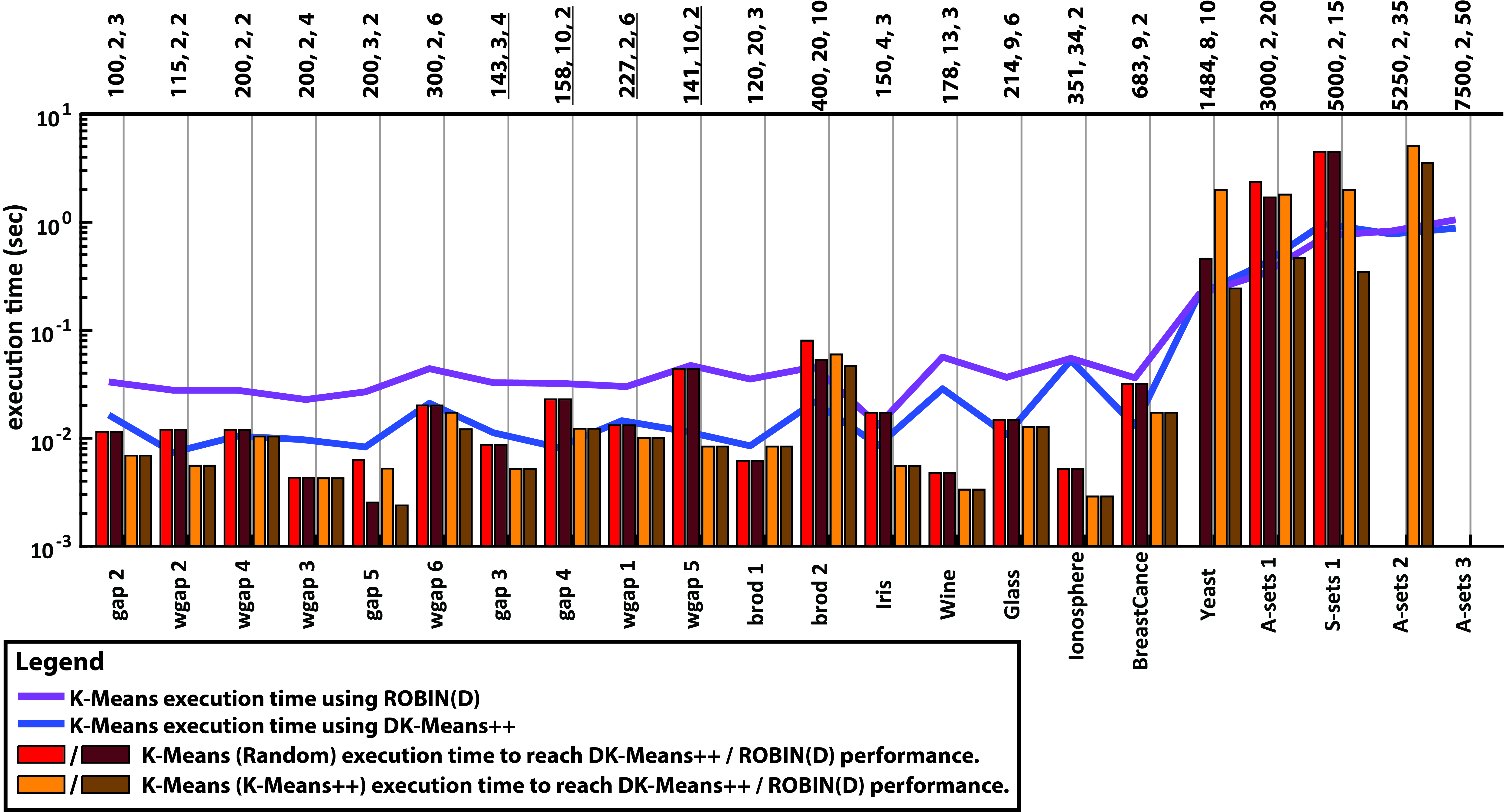
Figure 8: Execution time until stochastic methods reach or surpass the performance of deterministic methods. Each bar shows the running time requirements of the clustering algorithm initialised with a stochastic method to reach or surpass the performance of the same algorithm initialised with a deterministic method. The time requirements of the clustering algorithm using a deterministic method are shown as lines for comparison. Cases where bars are not shown mean that, up to 50 runs, the clustering algorithm using a stochastic method was unable to surpass the performance of the deterministic method.

We also investigated the number of iterations required for the clustering algorithm to reach convergence using stochastic and deterministic methods. We find that stochastic methods overall provide worst initial conditions (with the exception of ROBIN(S) vs Maximin(D)), and as a consequence the clustering algorithm requires more iterations to converge, which adds to the overhead of the stochastic initialisation methods (for results refer to the supplementary material).

5 Discussion

K-Means clustering remains one of the most common clustering techniques in many different research fields and frequently it is used as a component of more complex algorithms (e.g. hierarchical clustering [2]). Following similar benchmark studies on K-Means [6, 20, 13], in this study we compare stochastic and deterministic initialisation methods on K-Means variations. We particularly investigated the methods of ROBIN and DK-Means++ since to the best of our knowledge they have not been studied as extensively as other initialisation methods. Experimentally we showed:

• More sophisticated initialisation methods can lead, on average, to better clustering regardless of the K-Means variation (see Table 4). From the stochastic methods, ROBIN(S) can achieve the best average performance compared with Random, K-Means++ and Maximin(S) (see Figure 2). From the deterministic methods, DK-Means++ can achieve the best performance compared with Kaufman, Maximin(D) and ROBIN(D) (see Figure 3). In addition, DK-Means++ can achieve better performance from the average performance of stochastic methods (see Figure 4). Overall, deterministic methods have on average less performance variability across the data sets of each model we tested and lead to more stable solutions than stochastic methods (see supplementary material) and can surpass the performance of stochastic methods (see Figure 4).

• When executed multiple times stochastic methods can achieve better performance than deterministic methods. Opposite the the first point, in that case, less sophisticated methods (such as Random and K-Means++ as opposed to ROBIN(S)) can achieve better performance (see Figure 6). K-Means++ with 50 executions achieved the best performance followed by Random (see Figure 5). The only deterministic method that can still compete to an extent is DK-Means++ (see supplementary material where we provide a full list of all comparisons among all the initialisation methods).

• We found (see Table 5) that as indicated by [3] Hartigan-Wong K-Means is better than Lloyd’s K-Means and as shown by [43] (only for one K-Means variant) K-Medians is better than both Hartigan-Wong and Lloyd’s K-Means. However these differences add up to performance difference of only $1.5\%$ as measured by the purity index.

• Regarding execution time requirements, Random and K-Means++ are fastest performers in terms of single runs while Kaufman the slowest (see Figure 7). Maximin(S) is slightly slower than K-Means++. Nevertheless these methods require multiple executions in order to reach the performance of determinsitic methods (refer to Table 6) especially with bigger data sets (number of elements to thousands). Multiple executions of these methods have almost similar requirements as a single run of deterministic methods DK-Means++ and ROBIN(D) (refer to Figure 8). This is due to the fact that the clustering algorithm requires more iterations to reach converge when stochastic methods are used (refer to the supplementary material). Between DK-Means++ and ROBIN(D) the former is faster than the latter.

Overall, and from a practical point of view, the stochastic Random and the deterministic Kaufman methods are not advisable. The first method despite being the simplest and the fastest can be replaced with K-Means++ that has better probability of achieving superior performance. The latter method is extremely slow and there are better alternatives such as the DK-Means++ that has both better performance and execution time. Maximin(D) and ROBIN(S) are not advisable either since the former is relatively fast and multiple executions of Maximin(S) can be performed instead while the latter has much more time requirements, small variability on its solutions and when an approximate clustering is required ROBIN(D) can be used instead. DK-Means++ is a good option when determinism is required since with a single run it can achieve better performance compared with other dete trministic methods and comparable performance to multiple executions of stochastic methods that would require the same or more running time. In applications where exhausted search of optimal initial centroids needs to be performed K-Means++ should be considered (the study of [6] has also benchmarked a greedy version of this method which is also recommended). In these cases, if time requirements are flexible, a strategy would be to perform first DK-Means++ which would give an indication about the clustering capabilities of the data set and then multiple executions of K-Means++. We should add that in the mixed model 4, ROBIN(S) and ROBIN(D) performed significantly low compared with other cases because both where placing two initial centroids on the sides of the most elongated cluster while DK-Means++ were placing correctly a centroid almost in the middle of the cluster. This indicates that the DK-Means++’s heuristic might be more robust to applications than the LOF score of ROBIN for clusters detection. It should be noted that more complex techniques like DK-Means++ can be considered as clustering algorithms themselves since they produce good initial clusters. This observation was mentioned in the study of [6] and we also performed a study (refer to the supplementary material) on the number of iterations until the K-Means algorithm reaches convergence when it is initialized with different methods. Based on the results deterministic methods cause K-Means to converge faster than when it is initialized with stochastic methods. As expected, ROBIN(S) and DK-Means++ were again the best stochastic and deterministic methods on that account.

These conclusions were based on extensive benchmarking considering many different clustering models from other studies: Gaussian, high-dimensional (10 dimensions), elongated, unbalanced, non-Gaussian from the studies of [35] and [36]; high-dimensional (20 dimensions) containing informative and uninformative features and higher-dimensional (1000 and 1500 dimensions) with varying number of clusters (3, 10, 50 clusters) and cluster sizes (50-100 points) [12]. We also used our own models which contain clusters with different properties (unbalanced, elongated and Gaussian; unbalanced Gaussian and non-Gaussian; unbalanced, Gaussian with different variability among their dimensions).

With the use of synthetic data set generators we had the ability to generate multiple data sets and run hypothesis testing to further strengthen our conclusions but we also considered standalone data sets. The “clustering data sets” S-sets [37] and A-sets [38] were selected from the studies of [20, 13] because both are containing more clusters and data points than the generated ones and also because in the case of the S-sets the clusters are having different overlap degrees. The conclusions we obtained from the data set generators match with the conclusions of the standalone S-sets and A-sets data sets. Specifically for our higher dimensional data sets (1000, 1500 dimensions) generated using the Brodinova generator [12] (see Table 2) we selected to have small clusters due to the Kaufman initialization method which requires significant amount of time to be executed. However, we also generated data sets with larger clusters (approximately five times bigger) and we tested the ROBIN(D) and DK-Means++ methods on them. The results (not shown) and conclusions were similar to the ones reported already.

Based on the previous studies [20, 13] the authors have clearly demonstrated that K-Means performs worse when there is large number of clusters and that dimensionality does not have a direct effect on the performance of the algorithm. In our experiments using the Brodinova models (see Figures 3, 6 brod 1 to brod 12) we observe that indeed the performance of all the methods drops when the number of clusters is increased regardless of the dimensionality, especially in the case of Brodinova brod10 model where we generate data sets having 50 clusters. Apart from the last extreme case, we observed that multiple executions of stochastic methods improve the performance of K-Means. It should also be noted that the deterministic DK-Means++ method achieves (similar to multiple executions of stochastic methods i.e. Random, K-Means++, Maximin(S) and ROBIN(S)) the highest performance on the clustering basic benchmark [20, 13] in all the cases (see the supplementary material) even though these data sets have high number of clusters (A-sets: 20, 30, 50; S-sets: 15). The same authors [20, 13] also demonstrated that strong cluster unbalances affect negatively the K-Means clustering. In our experiments and specifically for the weighted gap 2 model we observed that data sets with unbalanced clusters do not cause any particular issues to the maximum performances of the algorithms. For the performance between K-Means and K-Medians, similar to the results of [43], we found that K-Medians outperforms K-Means on synthetic data set models but on a small difference of $1\%$ of purity and on standalone data sets (both synthetic and real-world) any particular differences among the K-Means variations couldn’t be clearly detected.

In order to show application to “real world problems” previous studies have chosen to use standard classification data sets as benchmarks for clustering. While this approach is commonly used, in these data the mapping from classes to clusters is somehow forced: it is possible that data from one class belong to different clusters, and assuming that number of clusters equals number of classes is likely to underestimate the true number of clusters. This can be seen from the low value of the Silhouette index especially in the cases of Ionosphere and Yeast data sets. For this we base our conclusions mostly on the benchmark models that allows us to generate multiple samples and evaluate the statistical significance of the results. In fact, we considered a broad combination of different clusters, in terms of normality (Gaussian, non-Gaussian), shape (spherical, elongated) and size (clusters with different number of data points) including high dimensional data, as found in real world applications such as bioinformatics [44].

It should also be noted that many clustering frameworks designed to deal with complex data sets (e.g. sub-clustering [45], or sparse clustering [7, 8, 12]) are using the K-Means or some variant of it and are dependent on good clustering initialisation. Our experimental work revealed that there are deterministic methods (DK-Means++ [18]) that lead to a good clustering solution with a single execution of the K-Means algorithm.

A limitation of the current study is that the execution time analysis is subject to the machine that executed it. More powerful machines or code optimisation of the algorithms and initialisation methods can change time analysis results. Nevertheless the rest of the analysis including the number of different seeds for stochastic methods to reach the performance of deterministic is, on average, reproducible. Statistics on average performance comparison are representative since, the analysis of sections 4.1, 4.2 and 4.3 had been also performed on 25 instances of the various data sets models instead of 50 and led to the same conclusions.

Contributions

A.V. performed the experiments and wrote the manuscript. E.V. contributed to the statistical and algorithmic analysis, provided feedback and edited the manuscript. S.L. oversaw the benchmarking process, provided feedback on the results presentation and the manuscript. M.C. contributed to the literature review and the discussion and performed the final proofreading.

Table 1: Summary of comparisons on average performance of stochastic and deterministic methods over different K-Means variations on synthetic data set models. In the first part of the table, each row compares two different methods over the Hartigan-Wong’s K-Means (HW), Lloyd’s K-Means (Ll) and K-Medians (KMed) algorithms on 26 occasions (10 gap and weighted gap, 12 Brodinova and 4 mixed models). The comparison is separate among the stochastic and deterministic methods and based on the times that there was significant difference between the two methods over the 40 data sets of each model. Based on the results ROBIN(S) is the best performer of stochastic methods and DK-Means the best performer of deterministic methods, both over all the clustering algorithms. The second part of the table groups all the stochastic and deterministic methods together and counts the overall percentage of observed significant differences. Based on the results the performance differences among the deterministic methods are less compared to the stochastic methods suggesting less performance variability. This Table accompanies Figure 2 and Figure 3 of the main manuscript which show the average performance of the initialisation methods based on Silhouette and show comparisons only for the Hartigan-Wong’s algorithm.

		Significant better average performance Silhouette (Purity)
Initialization method	Total number of instances	HW	Ll	KMed
Random vs K-Means++	26	0 vs 23 (0 vs 21)	0 vs 23 (0 vs 22)	0 vs 23 (0 vs 24)
Random vs ROBIN(S)	26	1 vs 22 (1 vs 22)	3 vs 22 (3 vs 22)	2 vs 23 (2 vs 23)
Random vs Maximin(S)	26	0 vs 17 (6 vs 15)	1 vs 19 (6 vs 16)	1 vs 19 (6 vs 16)
K-Means++ vs ROBIN(S)	26	1 vs 22 (1 vs 21)	3 vs 22 (3 vs 21)	2 vs 23 (2 vs 22)
K-Means++ vs Maximin(S)	26	5 vs 14 (8 vs 12)	5 vs 16 (9 vs 14)	5 vs 15 (7 vs 13)
ROBIN(S) vs Maximin(S)	26	17 vs 1 (17 vs 1)	17 vs 3 (18 vs 3)	18 vs 1 (19 vs 1)
Kaufman vs DK-Means++	26	3 vs 8 (3 vs 9)	3 vs 9 (3 vs 10)	3 vs 7 (4 vs 8)
Kaufman vs ROBIN(D)	26	5 vs 8 (4 vs 8)	6 vs 8 (6 vs 6)	5 vs 6 (4 vs 6)
Kaufman vs Maximin(D)	26	8 vs 5 (8 vs 5)	10 vs 6 (10 vs 6)	9 vs 5 (9 vs 5)
DK-Means++ vs ROBIN(D)	26	2 vs 1 (4 vs 0)	5 vs 1 (6 vs 0)	4 vs 1 (6 vs 1)
DK-Means++ vs Maximin(D)	26	7 vs 0 (9 vs 0)	9 vs 0 (11 vs 0)	7 vs 0 (10 vs 1)
ROBIN(D) vs Maximin(D)	26	8 vs 1 (8 vs 1)	9 vs 1 (10 vs 1)	8 vs 1 (9 vs 1)
		Observed significant performance differences on average performance Silhouette (Purity)
Initialization methods	Total number of instances	HW	Ll	KMed
Stochastic: Random, K-Means++, ROBIN(S), Maximin(S)	156	78.8% (80.1%)	86.0% (87.8%)	84.6% (86.5%)
Deterministic: Kaufman, DK-Means++, ROBIN(D), Maximin(D)	156	36.0% (37.8%)	42.9% (44.2%)	36.0% (41.0%)

Table 2: Detailed comparison on the maximum performance of stochastic methods with the performance of deterministic methods. Each row compares a stochastic with a deterministic method over the Hartigan-Wong’s K-Means (HW), Lloyd’s K-Means (Ll) and K-Medians (KMed) algorithms on 26 occasions (10 gap and weighted gap, 12 Brodinova and 4 mixed models). The comparison is based on the times that there was significant difference between the two methods on their maximum performance. Based on the results stochastic methods are better that deterministic on achieving the best performance but the more sophisticated the stochastic method is the less performance difference it achieves compared with deterministc methods for which the opposite is observed. This Table accompanies Figure 5 and Figure 6 of the main manuscript which show the maximum performance of the initialisation methods and show comparisons only for the Hartigan-Wong’s algorithm.

Initialization method	Total number of instances	Significant better maximum performance Purity for best Silhouette
		HW	Ll	KMed
Random vs Kaufman	26	9 vs 3	9 vs 4	9 vs 4
Random vs DK-Means++	26	5 vs 3	4 vs 2	5 vs 3
Random vs ROBIN(D)	26	6 vs 3	8 vs 2	7 vs 2
Random vs Maximin(D)	26	10 vs 2	12 vs 1	11 vs 1
K-Means++ vs Kaufman	26	10 vs 0	12 vs 0	10 vs 0
K-Means++ vs DK-Means++	26	6 vs 2	6 vs 2	7 vs 2
K-Means++ vs ROBIN(D)	26	8 vs 2	9 vs 2	8 vs 2
K-Means++ vs Maximin(D)	26	10 vs 1	12 vs 1	11 vs 1
ROBIN(S) vs Kaufman	26	9 vs 4	8 vs 6	8 vs 4
ROBIN(S) vs DK-Means++	26	0 vs 2	1 vs 3	2 vs 2
ROBIN(S) vs ROBIN(D)	26	6 vs 0	6 vs 0	6 vs 0
ROBIN(S) vs Maximin(D)	26	8 vs 0	9 vs 1	9 vs 0
Maximin(S) vs Kaufman	26	9 vs 4	9 vs 4	8 vs 4
Maximin(S) vs DK-Means++	26	2 vs 4	2 vs 5	3 vs 5
Maximin(S) vs ROBIN(D)	26	4 vs 4	6 vs 4	4 vs 4
Maximin(S) vs Maximin(D)	26	9 vs 1	11 vs 1	10 vs 1

Table 3: Comparison of the initialisation methods on standalone clustering data sets based on Silhouette index. Each stochastic method (Random, K-Means++, ROBIN(S) and Maximin (S)) was executed 50 times and the minimum, maximum and mean performance is shown followed by the performance variation for three K-Means variations. For the maximum performance the cases where a method has achieved the maximum performance is shown in bold.

		K-Means (Hartigan-Wong)				K-Means (Lloyd)				K-Medians
		min	max	mean	std	min	max	mean	std	min	max	mean	std
A-sets 1	Random	0.446	0.595	0.521	0.029	0.475	0.595	0.518	0.031	0.434	0.57	0.507	0.036
	K-Means++	0.482	0.595	0.548	0.03	0.484	0.595	0.548	0.024	0.469	0.595	0.531	0.029
	ROBIN(S)	0.567	0.595	0.586	0.013	0.568	0.595	0.58	0.014	0.567	0.595	0.585	0.013
	Maximin(S)	0.52	0.595	0.56	0.019	0.519	0.595	0.56	0.023	0.499	0.595	0.553	0.03
	Kaufman	0.567	0.567	0.567	0	0.567	0.567	0.567	0	0.567	0.567	0.567	0
	DK-Means++	0.595	0.595	0.595	0	0.595	0.595	0.595	0	0.595	0.595	0.595	0
	ROBIN(D)	0.567	0.567	0.567	0	0.568	0.568	0.568	0	0.567	0.567	0.567	0
	Maximin(D)	0.556	0.556	0.556	0	0.556	0.556	0.556	0	0.538	0.538	0.538	0
A-sets 2	Random	0.475	0.568	0.523	0.022	0.444	0.551	0.515	0.022	0.433	0.569	0.506	0.027
	K-Means++	0.505	0.598	0.543	0.02	0.483	0.584	0.547	0.024	0.473	0.58	0.531	0.021
	ROBIN(S)	0.58	0.598	0.591	0.008	0.581	0.598	0.59	0.008	0.581	0.597	0.59	0.008
	Maximin(S)	0.504	0.574	0.54	0.019	0.5	0.58	0.536	0.022	0.49	0.575	0.536	0.022
	Kaufman	0.565	0.565	0.565	0	0.565	0.565	0.565	0	0.538	0.538	0.538	0
	DK-Means++	0.598	0.598	0.598	0	0.598	0.598	0.598	0	0.597	0.597	0.597	0
	ROBIN(D)	0.598	0.598	0.598	0	0.598	0.598	0.598	0	0.597	0.597	0.597	0
	Maximin(D)	0.555	0.555	0.555	0	0.555	0.555	0.555	0	0.56	0.56	0.56	0
A-sets 3	Random	0.478	0.556	0.519	0.019	0.465	0.551	0.512	0.018	0.457	0.552	0.502	0.021
	K-Means++	0.514	0.588	0.547	0.017	0.506	0.601	0.548	0.017	0.485	0.576	0.533	0.019
	ROBIN(S)	0.601	0.601	0.601	0	0.601	0.601	0.601	0	0.601	0.601	0.601	0
	Maximin(S)	0.525	0.585	0.556	0.016	0.525	0.589	0.558	0.015	0.52	0.586	0.559	0.017
	Kaufman	0.53	0.53	0.53	0	0.53	0.53	0.53	0	0.529	0.529	0.529	0
	DK-Means++	0.601	0.601	0.601	0	0.601	0.601	0.601	0	0.601	0.601	0.601	0
	ROBIN(D)	0.601	0.601	0.601	0	0.601	0.601	0.601	0	0.601	0.601	0.601	0
	Maximin(D)	0.588	0.588	0.588	0	0.588	0.588	0.588	0	0.588	0.588	0.588	0
S-sets 1	Random	0.52	0.711	0.616	0.037	0.545	0.663	0.612	0.035	0.497	0.662	0.587	0.047
	K-Means++	0.58	0.711	0.654	0.039	0.529	0.711	0.655	0.044	0.517	0.711	0.651	0.044
	ROBIN(S)	0.711	0.711	0.711	0	0.711	0.711	0.711	0	0.711	0.711	0.711	0
	Maximin(S)	0.611	0.711	0.676	0.036	0.575	0.711	0.66	0.038	0.58	0.711	0.648	0.038
	Kaufman	0.711	0.711	0.711	0	0.638	0.638	0.638	0	0.654	0.654	0.654	0
	DK-Means++	0.711	0.711	0.711	0	0.711	0.711	0.711	0	0.711	0.711	0.711	0
	ROBIN(D)	0.711	0.711	0.711	0	0.711	0.711	0.711	0	0.711	0.711	0.711	0
	Maximin(D)	0.651	0.651	0.651	0	0.651	0.651	0.651	0	0.652	0.652	0.652	0
S-sets 2	Random	0.464	0.626	0.555	0.034	0.486	0.626	0.571	0.036	0.407	0.626	0.53	0.055
	K-Means++	0.516	0.626	0.586	0.031	0.505	0.626	0.577	0.032	0.485	0.626	0.566	0.035
	ROBIN(S)	0.575	0.626	0.617	0.02	0.575	0.626	0.61	0.024	0.568	0.626	0.606	0.028
	Maximin(S)	0.533	0.626	0.595	0.033	0.546	0.626	0.577	0.022	0.503	0.626	0.569	0.027
	Kaufman	0.57	0.57	0.57	0	0.57	0.57	0.57	0	0.571	0.571	0.571	0
	DK-Means++	0.626	0.626	0.626	0	0.626	0.626	0.626	0	0.626	0.626	0.626	0
	ROBIN(D)	0.626	0.626	0.626	0	0.626	0.626	0.626	0	0.626	0.626	0.626	0
	Maximin(D)	0.529	0.529	0.529	0	0.526	0.526	0.526	0	0.521	0.521	0.521	0
S-sets 3	Random	0.412	0.492	0.461	0.019	0.427	0.493	0.463	0.018	0.395	0.493	0.455	0.022
	K-Means++	0.431	0.492	0.467	0.018	0.429	0.493	0.465	0.017	0.409	0.493	0.459	0.02
	ROBIN(S)	0.431	0.466	0.462	0.01	0.452	0.467	0.464	0.005	0.423	0.468	0.457	0.015
	Maximin(S)	0.431	0.492	0.469	0.018	0.427	0.492	0.469	0.019	0.422	0.493	0.469	0.021
	Kaufman	0.492	0.492	0.492	0	0.492	0.492	0.492	0	0.493	0.493	0.493	0
	DK-Means++	0.493	0.493	0.493	0	0.493	0.493	0.493	0	0.493	0.493	0.493	0
	ROBIN(D)	0.466	0.466	0.466	0	0.467	0.467	0.467	0	0.464	0.464	0.464	0
	Maximin(D)	0.457	0.457	0.457	0	0.464	0.464	0.464	0	0.471	0.471	0.471	0
S-sets 4	Random	0.426	0.48	0.467	0.012	0.434	0.48	0.465	0.012	0.4	0.479	0.45	0.021
	K-Means++	0.431	0.48	0.469	0.012	0.433	0.48	0.469	0.012	0.412	0.479	0.456	0.017
	ROBIN(S)	0.457	0.48	0.468	0.007	0.435	0.47	0.458	0.012	0.45	0.466	0.461	0.006
	Maximin(S)	0.443	0.48	0.47	0.007	0.456	0.471	0.468	0.004	0.438	0.479	0.456	0.014
	Kaufman	0.48	0.48	0.48	0	0.48	0.48	0.48	0	0.458	0.458	0.458	0
	DK-Means++	0.48	0.48	0.48	0	0.48	0.48	0.48	0	0.479	0.479	0.479	0
	ROBIN(D)	0.48	0.48	0.48	0	0.435	0.435	0.435	0	0.466	0.466	0.466	0
	Maximin(D)	0.47	0.47	0.47	0	0.469	0.469	0.469	0	0.462	0.462	0.462	0

Table 4: Comparison of the initialisation methods on real-world data sets based on Silhouette index. Each stochastic method (Random, K-Means++, ROBIN(S) and Maximin (S)) was executed 50 times and the minimum, maximum and mean performance is shown followed by the performance variation for three K-Means variations. For the maximum performance the cases where a method has achieved the maximum performance is shown in bold.

		K-Means (Hartigan-Wong)				K-Means (Lloyd)				K-Medians
		min	max	mean	std	min	max	mean	std	min	max	mean	std
Iris	Random	0.517	0.553	0.549	0.012	0.5	0.553	0.543	0.016	0.467	0.551	0.542	0.016
	K-Means++	0.517	0.553	0.551	0.009	0.5	0.553	0.548	0.011	0.526	0.551	0.55	0.006
	ROBIN(S)	0.553	0.553	0.553	0	0.551	0.551	0.551	0	0.551	0.551	0.551	0
	Maximin(S)	0.553	0.553	0.553	0	0.551	0.553	0.552	0.001	0.551	0.551	0.551	0
	Kaufman	0.553	0.553	0.553	0	0.551	0.551	0.551	0	0.551	0.551	0.551	0
	DK-Means++	0.553	0.553	0.553	0	0.551	0.551	0.551	0	0.551	0.551	0.551	0
	ROBIN(D)	0.553	0.553	0.553	0	0.551	0.551	0.551	0	0.551	0.551	0.551	0
	Maximin(D)	0.553	0.553	0.553	0	0.553	0.553	0.553	0	0.551	0.551	0.551	0
Ionosphere	Random	0.296	0.296	0.296	0	0.246	0.368	0.296	0.013	0.231	0.334	0.283	0.013
	K-Means++	0.296	0.296	0.296	0	0.266	0.296	0.295	0.006	0.246	0.408	0.286	0.015
	ROBIN(S)	0.296	0.296	0.296	0	0.296	0.296	0.296	0	0.284	0.284	0.284	0
	Maximin(S)	0.296	0.296	0.296	0	0.295	0.408	0.314	0.038	0.284	0.408	0.311	0.05
	Kaufman	0.296	0.296	0.296	0	0.295	0.295	0.295	0	0.284	0.284	0.284	0
	DK-Means++	0.296	0.296	0.296	0	0.296	0.296	0.296	0	0.284	0.284	0.284	0
	ROBIN(D)	0.296	0.296	0.296	0	0.296	0.296	0.296	0	0.284	0.284	0.284	0
	Maximin(D)	0.296	0.296	0.296	0	0.296	0.296	0.296	0	0.284	0.284	0.284	0
Wine	Random	0.548	0.571	0.57	0.005	0.54	0.571	0.57	0.005	0.566	0.571	0.568	0.002
	K-Means++	0.548	0.571	0.562	0.01	0.548	0.571	0.566	0.007	0.566	0.571	0.57	0.002
	ROBIN(S)	0.571	0.571	0.571	0	0.571	0.571	0.571	0	0.566	0.566	0.566	0
	Maximin(S)	0.553	0.571	0.558	0.008	0.553	0.571	0.561	0.005	0.571	0.571	0.571	0
	Kaufman	0.571	0.571	0.571	0	0.571	0.571	0.571	0	0.571	0.571	0.571	0
	DK-Means++	0.571	0.571	0.571	0	0.571	0.571	0.571	0	0.571	0.571	0.571	0
	ROBIN(D)	0.571	0.571	0.571	0	0.571	0.571	0.571	0	0.566	0.566	0.566	0
	Maximin(D)	0.548	0.548	0.548	0	0.56	0.56	0.56	0	0.571	0.571	0.571	0
Breast Cancer	Random	0.597	0.597	0.597	0	0.597	0.597	0.597	0	0.597	0.597	0.597	0
	K-Means++	0.597	0.597	0.597	0	0.597	0.597	0.597	0	0.597	0.597	0.597	0
	ROBIN(S)	0.597	0.597	0.597	0	0.597	0.597	0.597	0	0.597	0.597	0.597	0
	Maximin(S)	0.597	0.597	0.597	0	0.597	0.597	0.597	0	0.597	0.597	0.597	0
	Kaufman	0.597	0.597	0.597	0	0.597	0.597	0.597	0	0.597	0.597	0.597	0
	DK-Means++	0.597	0.597	0.597	0	0.597	0.597	0.597	0	0.597	0.597	0.597	0
	ROBIN(D)	0.597	0.597	0.597	0	0.597	0.597	0.597	0	0.597	0.597	0.597	0
	Maximin(D)	0.597	0.597	0.597	0	0.597	0.597	0.597	0	0.597	0.597	0.597	0
Glass	Random	0.192	0.456	0.43	0.056	0.194	0.452	0.345	0.09	0.137	0.442	0.268	0.077
	K-Means++	0.271	0.587	0.457	0.053	0.278	0.585	0.454	0.064	0.211	0.592	0.432	0.089
	ROBIN(S)	0.447	0.452	0.447	0.001	0.43	0.448	0.443	0.005	0.257	0.397	0.384	0.028
	Maximin(S)	0.555	0.587	0.582	0.009	0.43	0.585	0.563	0.048	0.433	0.592	0.576	0.03
	Kaufman	0.452	0.452	0.452	0	0.448	0.448	0.448	0	0.238	0.238	0.238	0
	DK-Means++	0.447	0.447	0.447	0	0.431	0.431	0.431	0	0.435	0.435	0.435	0
	ROBIN(D)	0.447	0.447	0.447	0	0.444	0.444	0.444	0	0.392	0.392	0.392	0
	Maximin(D)	0.584	0.584	0.584	0	0.583	0.583	0.583	0	0.58	0.58	0.58	0
Yeast	Random	0.142	0.155	0.155	0.011	0.136	0.156	0.155	0.011	0.117	0.175	0.144	0.012
	K-Means++	0.15	0.217	0.177	0.012	0.148	0.192	0.173	0.01	0.119	0.184	0.157	0.013
	ROBIN(S)	0.18	0.183	0.181	0.001	0.178	0.19	0.183	0.006	0.161	0.172	0.164	0.005
	Maximin(S)	0.189	0.224	0.202	0.01	0.173	0.225	0.204	0.014	0.166	0.213	0.194	0.018
	Kaufman	0.161	0.161	0.161	0	0.159	0.159	0.159	0	0.151	0.151	0.151	0
	DK-Means++	0.155	0.155	0.155	0	0.156	0.156	0.156	0	0.14	0.14	0.14	0
	ROBIN(D)	0.183	0.183	0.183	0	0.19	0.19	0.19	0	0.172	0.172	0.172	0
	Maximin(D)	0.192	0.192	0.192	0	0.191	0.191	0.191	0	0.175	0.175	0.175	0

Initialization method	Total number of instances	Significantly more iterations for K-Means to converge
Random vs K-Means++	26	23 vs 0
Random vs ROBIN(S)	26	24 vs 0
Random vs Kaufman	26	23 vs 0
Random vs DK-Means++	26	25 vs 0
Random vs ROBIN(D)	26	24 vs 0
Random vs Maximin(S)	26	23 vs 2
Random vs Maximin(D)	26	23 vs 0
K-Means++ vs ROBIN(S)	26	22 vs 0
K-Means++ vs Kaufman	26	21 vs 2
K-Means++ vs DK-Means++	26	24 vs 0
K-Means++ vs ROBIN(D)	26	22 vs 0
K-Means++ vs Maximin(S)	26	21 vs 3
K-Means++ vs Maximin(D)	26	19 vs 1
ROBIN(S) vs Kaufman	26	11 vs 7
ROBIN(S) vs DK-Means++	26	14 vs 0
ROBIN(S) vs ROBIN(D)	26	3 vs 2
ROBIN(S) vs Maximin(S)	26	1 vs 21
ROBIN(S) vs Maximin(D)	26	1 vs 19
Kaufman vs DK-Means++	26	8 vs 4
Kaufman vs ROBIN(D)	26	7 vs 10
Kaufman vs Maximin(S)	26	3 vs 15
Kaufman vs Maximin(D)	26	3 vs 14
DK-Means++ vs ROBIN(D)	26	0 vs 15
DK-Means++ vs Maximin(S)	26	0 vs 20
DK-Means++ vs Maximin(D)	26	1 vs 18
ROBIN(D) vs Maximin(S)	26	1 vs 21
ROBIN(D) vs Maximin(D)	26	1 vs 17
Maximin(S) vs Maximin(D)	26	8 vs 1

Table 5: Summary of comparisons for the number of iterations until convergence for the Lloyd’s K-Means algorithm using different initialisation methods. Each row shows a comparison between different initialisation methods on the number of times that each method resulted on the Lloyd’s K-Means algorithm to have greater number of iterations until convergence. As indicator of performance, a method resulted to lower number of iterations is consider better, thus the lower the score the better the methods. Based on the results, ROBIN(S) is the best stochastic method and results to the less iterations for the K-Means algorithm to reach convergence; DK-Means++ is the best deterministic method and results to the less iterations for the K-Means algorithm to reach convergence. Overall, deterministic methods result to lower number of iterations for the K-Means algorithm.

Details about the Gaussian data sets of gap and weighted gap studies

• gap model 2: means of the cluster centers are as follows: [0,0], [0,5], [5,-3]. Standard deviation of all the centers is 1.

• gap model 3: means of the cluster centers are all randomly selected as N(0, 5$I$).

• weighted gap model 1: means of the cluster centers are as follows: [10,0], [6,0], [0,0], [-5, 0], [5, 5], [0, -6]. Standard deviation of all the centers is 1.

• weighted gap model 6: means of the cluster centers are as follows: [0,0], [-1,5], [10,-10], [15,-10], [10,-15], [25,25]. Standard deviation of all the centers is 1.

• gap model 4: means of the cluster centers are all randomly selected as N(0, 1.9$I$).

• weighted gap model 5: means of the cluster centers are all randomly selected as N(0, 3.6$I$).

• gap model 5: clusters where consisted of 100 points generated from 3 features with values equally spaced from -0.5 to 0.5 and the addition of Gaussian noise with standard deviation of 0.1. The values on all three dimensions of the second cluster was then increased by 10.

• weighted gap model 4: Similar to gap model 5 but the values of the second cluster were decreased by 1.

$I$ refers to the identity matrix with size equal to the dimensionality of the data set. Any data set with distance between clusters less than 1 was discarded and regenerated.

References

- [1] José M Pena, Jose Antonio Lozano, and Pedro Larranaga. An empirical comparison of four initialization methods for the k-means algorithm. Pattern recognition letters, 20(10):1027–1040, 1999.
- [2] Anil K Jain. Data clustering: 50 years beyond k-means. Pattern recognition letters, 31(8):651–666, 2010.
- [3] Noam Slonim, Ehud Aharoni, and Koby Crammer. Hartigan’s k-means versus lloyd’s k-means-is it time for a change? In IJCAI, pages 1677–1684, 2013.
- [4] John A Hartigan. Clustering algorithms. 1975.
- [5] C Aggarwal Charu and K REDDY Chandan. Data clustering: algorithms and applications, 2013.
- [6] M Emre Celebi, Hassan A Kingravi, and Patricio A Vela. A comparative study of efficient initialization methods for the k-means clustering algorithm. Expert systems with applications, 40(1):200–210, 2013.
- [7] Daniela M Witten and Robert Tibshirani. A framework for feature selection in clustering. Journal of the American Statistical Association, 105(490):713–726, 2010.
- [8] Yumi Kondo, Matias Salibian-Barrera, Ruben Zamar, et al. Rskc: an r package for a robust and sparse k-means clustering algorithm. Journal of Statistical Software, 72(5):1–26, 2016.
- [9] Mikhail Bilenko, Sugato Basu, and Raymond J Mooney. Integrating constraints and metric learning in semi-supervised clustering. In Proceedings of the twenty-first international conference on Machine learning, page 11. ACM, 2004.
- [10] Avgoustinos Vouros and Eleni Vasilaki. A semi-supervised sparse k-means algorithm. Pattern Recognition Letters, 142:65–71, 2021.
- [11] Mohammad Al Hasan, Vineet Chaoji, Saeed Salem, and Mohammed J Zaki. Robust partitional clustering by outlier and density insensitive seeding. Pattern Recognition Letters, 30(11):994–1002, 2009.
- [12] Šárka Brodinová, Peter Filzmoser, Thomas Ortner, Christian Breiteneder, and Maia Rohm. Robust and sparse k-means clustering for high-dimensional data. Advances in Data Analysis and Classification, pages 1–28, 2017.
- [13] Pasi Fränti and Sami Sieranoja. How much can k-means be improved by using better initialization and repeats? Pattern Recognition, 93:95–112, 2019.
- [14] James MacQueen et al. Some methods for classification and analysis of multivariate observations. In Proceedings of the fifth Berkeley symposium on mathematical statistics and probability, volume 1, pages 281–297. Oakland, CA, USA, 1967.
- [15] David Arthur and Sergei Vassilvitskii. k-means++: The advantages of careful seeding. In Proceedings of the eighteenth annual ACM-SIAM symposium on Discrete algorithms, pages 1027–1035. Society for Industrial and Applied Mathematics, 2007.
- [16] Teofilo F Gonzalez. Clustering to minimize the maximum intercluster distance. Theoretical Computer Science, 38:293–306, 1985.
- [17] Leonard Kaufman and Peter J Rousseeuw. Finding groups in data: an introduction to cluster analysis, volume 344. John Wiley & Sons, 2009.
- [18] N Nidheesh, KA Abdul Nazeer, and PM Ameer. An enhanced deterministic k-means clustering algorithm for cancer subtype prediction from gene expression data. Computers in biology and medicine, 91:213–221, 2017.
- [19] John A Hartigan and Manchek A Wong. Algorithm as 136: A k-means clustering algorithm. Journal of the Royal Statistical Society. Series C (Applied Statistics), 28(1):100–108, 1979.
- [20] Pasi Fränti and Sami Sieranoja. K-means properties on six clustering benchmark datasets. Applied Intelligence, 48(12):4743–4759, 2018.
- [21] MATLAB. version 9.6.0 (R2019a). The MathWorks Inc., Natick, Massachusetts, 2019.
- [22] Guido van Rossum. Python tutorial, Technical Report CS-R9526. Centrum voor Wiskunde en Informatica (CWI), Amsterdam, 1995.
- [23] R Core Team. R: A Language and Environment for Statistical Computing. R Foundation for Statistical Computing, Vienna, Austria, 2013.
- [24] Dan Feldman and Leonard J Schulman. Data reduction for weighted and outlier-resistant clustering. In Proceedings of the twenty-third annual ACM-SIAM symposium on Discrete Algorithms, pages 1343–1354. Society for Industrial and Applied Mathematics, 2012.
- [25] Christopher Whelan, Greg Harrell, and Jin Wang. Understanding the k-medians problem. In Proceedings of the International Conference on Scientific Computing (CSC), page 219. The Steering Committee of The World Congress in Computer Science, Computer …, 2015.
- [26] Hendrik P Lopuhaa, Peter J Rousseeuw, et al. Breakdown points of affine equivariant estimators of multivariate location and covariance matrices. The Annals of Statistics, 19(1):229–248, 1991.
- [27] RC Jancey. Multidimensional group analysis. Australian Journal of Botany, 14(1):127–130, 1966.
- [28] Ioannis Katsavounidis, C-C Jay Kuo, and Zhen Zhang. A new initialization technique for generalized lloyd iteration. IEEE Signal processing letters, 1(10):144–146, 1994.
- [29] Markus M Breunig, Hans-Peter Kriegel, Raymond T Ng, and Jörg Sander. Lof: identifying density-based local outliers. In ACM sigmod record, volume 29, pages 93–104. ACM, 2000.
- [30] Alex Rodriguez and Alessandro Laio. Clustering by fast search and find of density peaks. Science, 344(6191):1492–1496, 2014.
- [31] Xv Lan, Qian Li, and Yi Zheng. Density k-means: A new algorithm for centers initialization for k-means. In Software Engineering and Service Science (ICSESS), 2015 6th IEEE International Conference on, pages 958–961. IEEE, 2015.
- [32] Bernard ME Moret and Henry D Shapiro. An empirical assessment of algorithms for constructing a minimum spanning tree. Computational Support for Discrete Mathematics, 15:99–117, 1992.
- [33] Eréndira Rendón, Itzel Abundez, Alejandra Arizmendi, and Elvia M Quiroz. Internal versus external cluster validation indexes. International Journal of computers and communications, 5(1):27–34, 2011.
- [34] Peter J Rousseeuw. Silhouettes: a graphical aid to the interpretation and validation of cluster analysis. Journal of computational and applied mathematics, 20:53–65, 1987.
- [35] Robert Tibshirani, Guenther Walther, and Trevor Hastie. Estimating the number of clusters in a data set via the gap statistic. Journal of the Royal Statistical Society: Series B (Statistical Methodology), 63(2):411–423, 2001.
- [36] Mingjin Yan and Keying Ye. Determining the number of clusters using the weighted gap statistic. Biometrics, 63(4):1031–1037, 2007.
- [37] P. Fränti and O. Virmajoki. Iterative shrinking method for clustering problems. Pattern Recognition, 39(5):761–765, 2006.
- [38] I. Kärkkäinen and P. Fränti. Dynamic local search algorithm for the clustering problem. Technical Report A-2002-6, Department of Computer Science, University of Joensuu, Joensuu, Finland, 2002.
- [39] Arthur Asuncion and David Newman. Uci machine learning repository, 2007.
- [40] Numerical Algorithms Group (NAG). The nag toolbox for matlab ®, 2019.
- [41] Tiago V Gehring, Gediminas Luksys, Carmen Sandi, and Eleni Vasilaki. Detailed classification of swimming paths in the morris water maze: multiple strategies within one trial. Scientific reports, 5:14562, 2015.
- [42] M Hahsler, M Piekenbrock, S Arya, and D Mount. dbscan: Density Based Clustering of Applications with Noise (DBSCAN) and Related Algorithms, 2019.
- [43] Michael J Brusco, Emilie Shireman, and Douglas Steinley. A comparison of latent class, k-means, and k-median methods for clustering dichotomous data. Psychological methods, 22(3):563, 2017.
- [44] Y Wang, DJ Miller, and R Clarke. Approaches to working in high-dimensional data spaces: gene expression microarrays. British journal of cancer, 98(6):1023, 2008.
- [45] Arijit Biswas and David Jacobs. Active subclustering. Computer Vision and Image Understanding, 125:72–84, 2014.