Dynamics and stability of chimera states in two coupled populations of oscillators

Abstract

We consider networks formed from two populations of identical oscillators, with uniform strength all-to-all coupling within populations, and also between populations, with a different strength. Such systems are known to support chimera states in which oscillators within one population are perfectly synchronised while in the other the oscillators are incoherent, and have a different mean frequency from those in the synchronous population. Assuming that the oscillators in the incoherent population always lie on a closed smooth curve $\mathcal{C}$, we derive and analyse the dynamics of the shape of $\mathcal{C}$ and the probability density on $\mathcal{C}$, for four different types of oscillators. We put some previously derived results on a rigorous footing, and analyse two new systems.

I Introduction

Chimera states in networks of coupled oscillators have been intensively studied in recent years panabr15 ; ome18 . Often they are studied in one-dimensional omeome13 ; abrstr06 ; abrstr04 ; kurbat02 or two-dimensional domains lai17 ; omewol12 ; panabr15a ; xiekno15 ; shikur04 ; marlai10 with nonlocal coupling, but it was Abrams et al. abrmir08 who first “coarse-grained” space and studied chimeras in a network formed from two populations of oscillators, with equal strength coupling between oscillators within a population, and weaker coupling to those in the other population. Later studies of networks with such structure include lai09a ; precha17 ; marbic16 ; panabr16 ; pikros08 and we also mention the experimental results tinnko12 ; marthu13 and the prior work monkur04 . In such networks a chimera state occurs when one population is perfectly synchronised (all oscillators behave identically) while in the other the oscillators are not phase synchronised but all have the same time-averaged frequency, which is different from that of the synchronous population. Such a state is similar to that of self-consistent partial synchrony clupol18 ; vre96 ; clupol16

Regarding the types of oscillators used, early works used phase oscillators with sinusoidal interaction functions abrstr06 ; abrstr04 , while later studies include oscillators near a SNIC bifurcation vulhiz14 , van der Pol oscillators omezak15 , oscillators with inertia boukan14 ; olm15 ; belbri16 , Stuart-Landau oscillators lai10 ; precha17 , and neuron models including leaky integrate-and-fire olmpol11 , quadratic integrate-and-fire ratpyr17 , and FitzHugh-Nagumo omeome13 .

The vast majority of papers concerning chimeras show just the results of numerical simulations of finite networks of oscillators. Early researchers showed the existence of chimeras using a self-consistency argument abrstr04 ; kurbat02 ; shikur04 ; marlai10 and later the Ott/Antonsen ansatz ottant08 was used to investigate their stability lai09 ; abrmir08 ; marbic16 ; omewol12 ; mar10 . However, these techniques relied on the number of oscillators being infinite, and more restrictively, that the oscillators were phase oscillators coupled through a purely sinusoidal function of phase differences. (Also, states found using the Ott/Antonsen ansatz are not attracting for networks of identical oscillators — heterogeneity is required to give stability lai09 ; lai17 .) Finite networks of identical sinusoidally coupled phase oscillators have been studied using the Watanabe/Strogatz ansatz watstr94 ; pikros08 ; panabr16 .

An exception to the approach above was lai10 , where chimeras in a network of two populations of Stuart-Landau oscillators were studied using a self-consistency argument. The existence of a chimera state was determined from the periodic solution of an ordinary differential equation (ODE), but this approach did not provide information on the stability or otherwise of the solution found.

In this paper we use techniques from clupol18 to revisit the system studied in lai10 and calculate stability information for the solutions found there. Since the approach in clupol18 is generally applicable to a situation in which oscillators in one population lie on a closed smooth curve, we then apply these ideas to three more networks formed from two coupled populations. The second network we consider consists of Kuramoto oscillators with inertia, each described by a second order ODE. The third network consists of FitzHugh-Nagumo neural oscillators, each described by a pair of ODEs. Unlike the oscillators studied in the first and second networks, these are not invariant under a global phase shift. The last network we consider consists of Stuart-Landau oscillators with delayed coupling both within and between populations.

We now briefly present the results from clupol18 which we will use. Sec. II contains the analysis and results for the four types of networks, while Sec. III contains a discussion and conclusion.

Clusella and Politi clupol18 consider a network of $N$ oscillators, with the state of the $j$th oscillator being described by the complex variable $z_{j}$. The dynamics is given by

$$\frac{dz_{j}}{dt}=f(z_{j},\bar{z};K)$$ (1)

for some function $f$ where the mean field is given by

$$\bar{z}=\frac{1}{N}\sum_{k=1}^{N}z_{k}$$ (2)

and $K$ is the strength of coupling between an oscillator and the mean field. For some values of $K$ it is observed that when the states of all oscillators are plotted as points in the complex plane, they lie on a smooth curve, $\mathcal{C}$, enclosing the origin, the shape of which is parametrised by an angle $\phi$. The distance from the origin to $\mathcal{C}$ at angle $\phi$ is $R(\phi,t)$, and the density at the point parametrised by $\phi$ is $P(\phi,t)$. Writing $z_{j}=r_{j}e^{i\phi_{j}}$ we can write (1) as

$$\frac{dr_{j}}{dt} =F(r_{j},\phi_{j},\bar{z})$$ (3)

$$\frac{d\phi_{j}}{dt} =G(r_{j},\phi_{j},\bar{z})$$ (4)

Clusella and Politi clupol18 show that the dynamics of $R$ and $P$ are given by

$$\frac{\partial R}{\partial t}(\phi,t) =F(R,\phi,\bar{z})-G(R,\phi,\bar{z})\frac{\partial R}{\partial\phi}$$ (5)

$$\frac{\partial P}{\partial t}(\phi,t) =-\frac{\partial}{\partial\phi}\left[P(\phi,t)G(R,\phi,\bar{z})\right]$$ (6)

where

$$\bar{z}=\int_{0}^{2\pi}P(\phi,t)R(\phi,t)e^{i\phi}d\phi$$ (7)

They used these equations to study the splay state and self-consistent partial synchrony in a network of Stuart-Landau oscillators. Of course, such equations are only a valid description of the dynamics of the network if the oscillators do lie on a curve $\mathcal{C}$, which should be checked by solving the original equations governing their dynamics. Numerically, we will treat $R$ and $P$ as continuous functions of $\phi$, corresponding to an infinite number of oscillators.

While clupol18 considered a single population of all-to-all coupled oscillators, the approach is also valid for a network of two populations of oscillators in which oscillators in one population lie on a smooth closed curve while those in the other population are perfectly synchronous, i.e. a chimera state. (It is also valid when oscillators from each population lie on their own curve; see Sec. II.3.)

II Results

II.1 Stuart-Landau oscillators

We first consider the chimera state found in lai10 . The equations governing the dynamics are

$$\frac{dX_{j}}{dt} =i\omega X_{j}+\epsilon^{-1}\{1-(1+\delta\epsilon i)|X_{j}|^{2}\}X_{j}+e^{-i\alpha}\left(\frac{\mu}{N}\sum_{k=1}^{N}X_{k}+\frac{\nu}{N}\sum_{k=1}^{N}X_{N+k}\right)$$ (8)

for $j=1,\dots N$ and

$$\frac{dX_{j}}{dt} =i\omega X_{j}+\epsilon^{-1}\{1-(1+\delta\epsilon i)|X_{j}|^{2}\}X_{j}+e^{-i\alpha}\left(\frac{\mu}{N}\sum_{k=1}^{N}X_{N+k}+\frac{\nu}{N}\sum_{k=1}^{N}X_{k}\right)$$ (9)

for $j=N+1,\dots 2N$, where each $X_{j}\in\mathbb{C}$ and $\omega,\epsilon,\delta,\alpha,\mu$ and $\nu$ are all real parameters. In a chimera state, $X_{j}=Y$ for $j\in\{N+1,\dots 2N\}$, i.e. population two is perfectly synchronised. Letting

$$\bar{X}=\frac{1}{N}\sum_{k=1}^{N}X_{k}$$ (10)

we have

$$\frac{dY}{dt}=i\omega Y+\epsilon^{-1}\{1-(1+\delta\epsilon i)|Y|^{2}\}Y+e^{-i\alpha}\left(\mu Y+\nu\bar{X}\right)$$ (11)

and each oscillator in population one satisfies

$$\frac{dX_{j}}{dt} =i\omega X_{j}+\epsilon^{-1}\{1-(1+\delta\epsilon i)|X_{j}|^{2}\}X_{j}+e^{-i\alpha}\left(\mu\bar{X}+\nu Y\right),$$ (12)

for $j=1,\dots N$. Writing $X_{j}=r_{j}e^{i\phi_{j}}$ we have

$$\frac{dr_{j}}{dt} =\epsilon^{-1}(1-r_{j}^{2})r_{j}+\mbox{Re}\left[e^{-i(\alpha+\phi_{j})}\left(\mu\bar{X}+\nu Y\right)\right]\equiv F(r_{j},\phi_{j},\bar{X},Y)$$ (13)

$$\frac{d\phi_{j}}{dt} =\omega-\delta r_{j}^{2}+\frac{1}{r_{j}}\mbox{Im}\left[e^{-i(\alpha+\phi_{j})}\left(\mu\bar{X}+\nu Y\right)\right]\equiv G(r_{j},\phi_{j},\bar{X},Y)$$ (14)

Thus we consider the dynamical system

$$\frac{\partial R}{\partial t}(\phi,t) =F(R,\phi,\bar{X},Y)-G(R,\phi,\bar{X},Y)\frac{\partial R}{\partial\phi}$$ (15)

$$\frac{\partial P}{\partial t}(\phi,t) =-\frac{\partial}{\partial\phi}\left[P(\phi,t)G(R,\phi,\bar{X},Y)\right]+D\frac{\partial^{2}}{\partial\phi^{2}}P(\phi,t)$$ (16)

$$\frac{dY}{dt} =i\omega Y+\epsilon^{-1}\{1-(1+\delta\epsilon i)|Y|^{2}\}Y+e^{-i\alpha}\left(\mu Y+\nu\bar{X}\right)$$ (17)

where

$$\bar{X}=\int_{0}^{2\pi}P(\phi,t)R(\phi,t)e^{i\phi}d\phi$$ (18)

and for numerical stability reasons we have added a small amount of diffusion, of strength $D$, to (6) (as did clupol18 ). The equations (15)-(18) form a coupled PDE/ODE system. We define $\beta=\pi/2-\alpha$ and let $\mu=(1+A)/2,\nu=(1-A)/2$.

Note that (8)-(9) are invariant under the global phase shift $X_{j}\mapsto X_{j}e^{i\gamma}$ for any constant $\gamma$ and thus we can move to a rotating coordinate frame in which $Y$ is constant, and we can then shift our coordinate system so that $Y$ is real. Moving to a coordinate frame rotating with speed $\Omega$ has the effect of replacing $\omega$ in (14) and (17) by $\omega+\Omega$.

We numerically integrate (15)-(18) in time to find a stable solution. An example is shown in Fig. 1. (Compare with Fig. 1 of lai10 .) We discretised $\phi$ using $256$ equally-spaced points and implemented derivatives with respect to $\phi$ spectrally tre00 . We enforce conservation of probability by setting $P$ at one grid point equal to $1/\Delta$ minus the sum of the values at all other grid points, where $\Delta=2\pi/256$, the $\phi$ grid spacing erm06 . We then follow the solution in Fig. 1 using pseudo-arclength continuation lai14 ; auto as $\epsilon$ is varied. The results are shown in Fig. 2, and we have reproduced the first four panels in Fig. 2 of lai10 . Note that stability is calculated from the eigenvalues of the linearisation of (15)-(18) about the steady state, unlike in lai10 where it was just inferred.

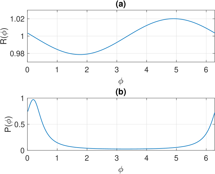
Figure 1: Snapshot of a solution of (15)-(18) for which $Y$ is real. (a): $R(\phi)$, (b): $P(\phi)$. Parameters: $\epsilon=0.05,\omega=0,\delta=-0.01,A=0.2,\beta=0.08,D=10^{-8}$.

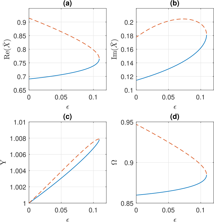
Figure 2: Steady states of (15)-(18) as functions of $\epsilon$. (a): Re($\bar{X}$), (b): Im($\bar{X}$), (c): $Y$ and (d): $\Omega$. Solid: stable; dashed: unstable. Other parameters: $\omega=0,\delta=-0.01,A=0.2,\beta=0.08,D=10^{-8}$.

The eigenvalues, $\lambda_{j}$, of the linearisation of (15)-(18) about the solution shown in Fig. 1 are plotted in the complex plane in Fig. 3. We notice that they form two clusters, one around Re$(\lambda_{j})=-40$ and the other around Re$(\lambda_{j})=0$. The first group can be understood by linearising $F$ with respect to $R$. We obtain $\epsilon^{-1}(1-3R^{2})$, and evaluating this at $R=1$ gives $-2/\epsilon=-40$, for this solution. The second group of eigenvalues is presumably related to the dynamics of $P$, and has been observed in other similar systems clupol16 ; clupol18 ; ome18 . The slight deviation from the imaginary axis visible in panel (c) of Fig. 3 is due to the non-zero value of $D$ used ($D=10^{-8}$). If $D$ is set to zero when calculating the eigenvalues, this group lies very close to the imaginary axis ($|\mbox{Re}(\lambda_{j})|<10^{-9}$).

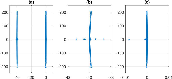
Figure 3: (a): spectrum of the solution shown in Fig. 1. Panels (b) and (c) show details of the two clusters of eigenvalues. Parameters: $\epsilon=0.05,\omega=0,\delta=-0.01,A=0.2,\beta=0.08,D=10^{-8}$.

As mentioned in clupol18 , one could find a steady state of (15)-(18) with $D=0$ by assuming a value for $\bar{X}$, solving $dY/dt=0$ for $Y$, numerically integrating

$$\frac{\partial R}{\partial\phi}=\frac{F(R,\phi,\bar{X},Y)}{G(R,\phi,\bar{X},Y)}$$ (19)

to obtain $R_{0}(\phi)$, setting

$$P_{0}(\phi)=\frac{\eta}{G(R_{0},\phi,\bar{X},Y)}$$ (20)

where $\eta$ is a normalisation constant (since $P$ is a probability density) and then requiring that

$$\int_{0}^{2\pi}P_{0}(\phi)R_{0}(\phi)e^{i\phi}d\phi$$ (21)

is equal to the value originally assumed for $\bar{X}$. Such an approach is equivalent to that taken in lai10 , where the equations governing a single oscillator in population one

$$\frac{dr}{dt} =F(r,\phi,\bar{X},Y)$$ (22)

$$\frac{d\phi}{dt} =G(r,\phi,\bar{X},Y)$$ (23)

were numerically solved in a self-consistent way to show the existence of a chimera.

Now each oscillator in population one satisfies (22)-(23). Thus having found a steady state of (15)-(18) by integrating these equations in time, we can find a periodic solution of (22)-(23). $2\pi$ divided by the period of this orbit then gives the angular frequency of an incoherent oscillator, relative to that of the synchronous group (whose frequency in the original coordinate frame is $\Omega$). For all of the points shown in Fig. 2, (22)-(23) has a stable periodic solution, the period of which is shown in Fig. 4. Note that this Figure reproduces panel (e) in Fig. 2 of lai10 .

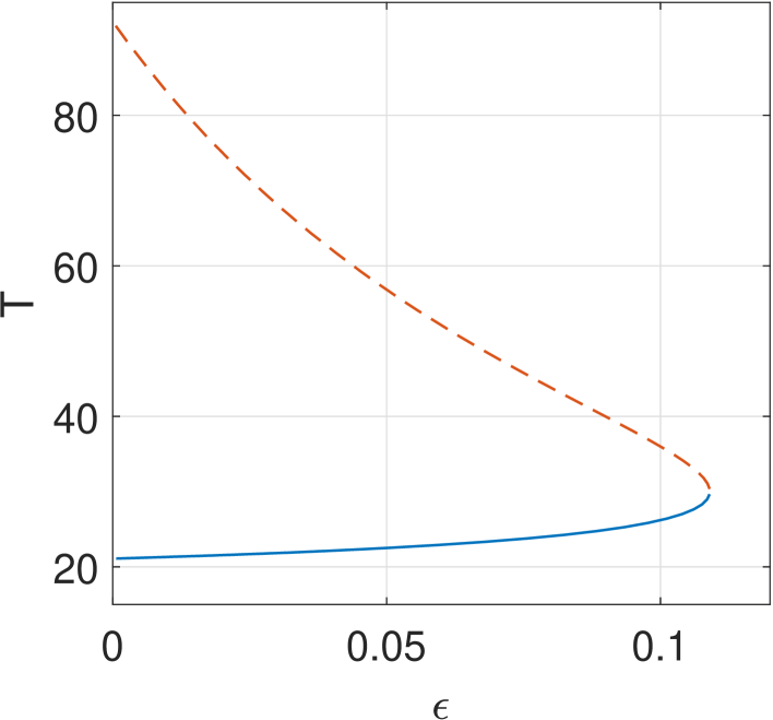
Figure 4: Period, $T$, of the stable periodic solution of (22)-(23), where the values of $\bar{X},Y$ and $\Omega$ are those shown in Fig. 2. Solid and dashed lines refer to stability indicated in Fig. 2. Other parameters: $\omega=0,\delta=-0.01,A=0.2,\beta=0.08,D=10^{-8}$.

Following the saddle-node bifurcation shown in Fig. 2 as $A$ is varied we obtain Fig. 5. By increasing $A$ for $\epsilon=0.05$ we find a Hopf bifurcation, also shown in Fig. 5. Numerical investigations suggest that this bifurcation is supercritical, and that the oscillations created in it are destroyed in a homoclinic bifurcation to the right of the Hopf curve in Fig. 5. The curve of homoclinic bifurcations should terminate at the codimension-two point where the Hopf curve meets the saddle-node curve; this scenario is observed in many systems showing chimeras lai10 ; lai09 ; abrmir08 ; panabr16 ; mar10 ; mar10a ; marbic16 . Note that the curve of Hopf bifurcations was found by following the algebraic equations defining such a bifurcation, whereas in lai10 , such a curve was found through direct simulation of (8)-(9).

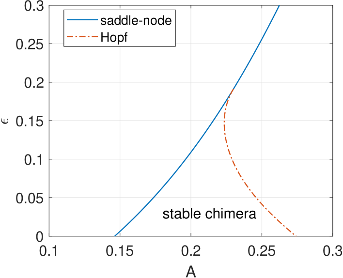
Figure 5: Continuation of the saddle-node bifurcation shown in Fig. 2 (solid) and a Hopf bifurcation (dash-dotted). Oscillating chimeras exist slightly to the right of the Hopf curve. Other parameters: $\omega=0,\delta=-0.01,\beta=0.08,D=10^{-8}$.

We end this section by noting that with the approach presented here we cannot detect bifurcations in which the synchronous group becomes asynchronous. Also, above the saddle-node curve in Fig. 5 the only attractor is the fully synchronous state and the approach presented here cannot be used to study this state, as $P$ approaches a delta function in $\phi$ and our numerical scheme breaks down.

II.2 Kuramoto with inertia

We now consider a network formed from two populations of $N$ Kuramoto oscillators with inertia. The system is described by

$$m\frac{d^{2}\theta_{i}^{(1)}}{dt^{2}}+\frac{d\theta_{i}^{(1)}}{dt} =\omega+\frac{\mu}{N}\sum_{j=1}^{N}\sin{\left(\theta_{j}^{(1)}-\theta_{i}^{(1)}-\alpha\right)}+\frac{\nu}{N}\sum_{j=1}^{N}\sin{\left(\theta_{j}^{(2)}-\theta_{i}^{(1)}-\alpha\right)}$$ (24)

$$m\frac{d^{2}\theta_{i}^{(2)}}{dt^{2}}+\frac{d\theta_{i}^{(2)}}{dt} =\omega+\frac{\mu}{N}\sum_{j=1}^{N}\sin{\left(\theta_{j}^{(2)}-\theta_{i}^{(2)}-\alpha\right)}+\frac{\nu}{N}\sum_{j=1}^{N}\sin{\left(\theta_{j}^{(1)}-\theta_{i}^{(2)}-\alpha\right)}$$ (25)

where $m$ is “mass”, $\omega,\mu,\nu$ and $\alpha$ are parameters, and the superscript labels the population. When $m=0$ this reverts to a previously studied case abrmir08 ; pikros08 . It is reasonable to expect that chimeras may exist and be stable for $m$ in some interval $[0,m_{0}]$, as found via numerical simulations of slightly heterogeneous oscillators boukan14 . Note that the system is invariant under a uniform shift of all of the phases, so we can set $\omega=0$ without loss of generality. We rewrite the equations as

$$\frac{d\theta_{i}^{(1)}}{dt} =u_{i}^{(1)}$$ (26)

$$\frac{du_{i}^{(1)}}{dt} =\left[-u_{i}^{(1)}+\frac{\mu}{N}\sum_{j=1}^{N}\sin{\left(\theta_{j}^{(1)}-\theta_{i}^{(1)}-\alpha\right)}+\frac{\nu}{N}\sum_{j=1}^{N}\sin{\left(\theta_{j}^{(2)}-\theta_{i}^{(1)}-\alpha\right)}\right]/m$$ (27)

$$\frac{d\theta_{i}^{(2)}}{dt} =u_{i}^{(2)}$$ (28)

$$\frac{du_{i}^{(2)}}{dt} =\left[-u_{i}^{(2)}+\frac{\mu}{N}\sum_{j=1}^{N}\sin{\left(\theta_{j}^{(2)}-\theta_{i}^{(2)}-\alpha\right)}+\frac{\nu}{N}\sum_{j=1}^{N}\sin{\left(\theta_{j}^{1}-\theta_{i}^{(2)}-\alpha\right)}\right]/m$$ (29)

In a chimera state let us assume that population two is fully synchronised, with $\theta_{i}^{(2)}=\Theta$ for $i=1,2\dots N$. This population satisfies

$$\frac{d\Theta}{dt} =U$$ (30)

$$\frac{dU}{dt} =\left[-U-\mu\sin{\alpha}+\frac{\nu}{N}\sum_{j=1}^{N}\sin{(\theta_{j}-\Theta-\alpha)}\right]/m$$

$$=\left[-U-\mu\sin{\alpha}+\nu\mbox{Im}\left\{e^{-i(\Theta+\alpha)}X\right\}\right]/m$$ (31)

where

$$X\equiv\frac{1}{N}\sum_{j=1}^{N}e^{i\theta_{j}}\in\mathbb{C},$$ (32)

the sums are over population one, and we have dropped the superscripts. Oscillators in population one satisfy

$$\frac{d\theta_{i}}{dt} =u_{i}$$ (33)

$$\frac{du_{i}}{dt} =\left[-u_{i}+\frac{\mu}{N}\sum_{j=1}^{N}\sin{(\theta_{j}-\theta_{i}-\alpha)}+\nu\sin{(\Theta-\theta_{i}-\alpha)}\right]/m$$

$$=\left[-u_{i}+\mu\mbox{Im}\left\{e^{-i(\theta_{i}+\alpha)}X\right\}+\nu\sin{(\Theta-\theta_{i}-\alpha)}\right]/m$$ (34)

We put these equations in “polar” form by defining $r_{j}=2+u_{j}$ and thus we have

$$\frac{dr_{j}}{dt} =\left[-(r_{j}-2)+\mu\mbox{Im}\left\{e^{-i(\theta_{i}+\alpha)}X\right\}+\nu\sin{(\Theta-\theta_{i}-\alpha)}\right]/m\equiv F(r_{j},\theta_{j},X,\Theta)$$ (35)

$$\frac{d\theta_{j}}{dt} =r_{j}-2$$ (36)

The chimera state of interest is stationary in a coordinate frame rotating at speed $\Omega$. Moving to this coordinate frame has the effect of replacing (30) by

$$\frac{d\Theta}{dt}=U+\Omega$$ (37)

and (36) by

$$\frac{d\theta_{j}}{dt}=r_{j}-2+\Omega\equiv G(r_{j},\theta_{j},X,\Theta)$$ (38)

Thus we consider the dynamical system

$$\frac{\partial R}{\partial t}(\theta,t) =F(R,\theta,X,\Theta)-G(R,\theta,X,\Theta)\frac{\partial R}{\partial\theta}$$ (39)

$$\frac{\partial P}{\partial t}(\theta,t) =-\frac{\partial}{\partial\theta}\left[P(\theta,t)G(R,\theta,X,\Theta)\right]+D\frac{\partial^{2}}{\partial\theta^{2}}P(\theta,t)$$ (40)

along with (31) and (37) where

$$X(t)=\int_{0}^{2\pi}P(\theta,t)R(\theta,t)e^{i\theta}d\theta$$ (41)

Choosing parameters $\mu=0.6,\nu=0.4,\alpha=\pi/2-0.05,m=0.1,D=10^{-4}$ and numerically integrating this system we find a stable steady state, shown in Fig. 6. However, decreasing $D$ from this value we find that this solution is actually unstable for smaller values of $D$, with the instability seeming to be a Hopf bifurcation.

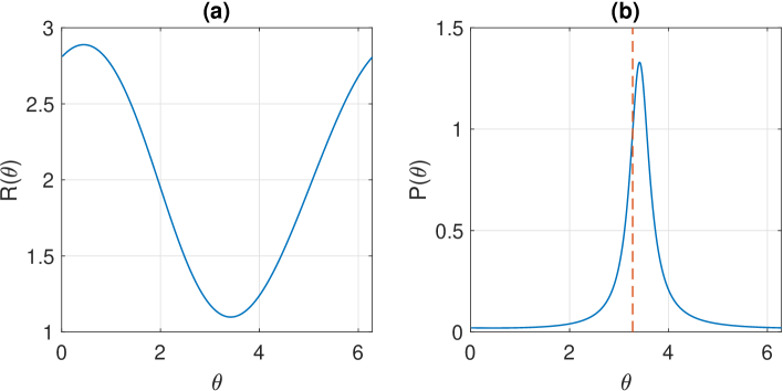
Figure 6: Steady state of (39)-(40), (31) and (37). (a): $R(\theta)$. (b): $P(\theta)$ (solid) with the value of $\Theta$ shown dotted. Parameters: $\mu=0.6,\nu=0.4,\alpha=\pi/2-0.05,m=0.1,D=10^{-4}$.

To verify this we followed the steady state shown in Fig. 6 as $m$ was varied, for a very small value of $D$ ($D=10^{-13}$). The real part of the right-most eigenvalues of the linearisation about this state are shown in Fig. 7, and we see that for all values of $m$, these are positive (and the right-most eigenvalues are a complex conjugate pair). Thus the system (39)-(40), (31) and (37) does not support a stable chimera for small values of $m$. (The system was discretised in $\theta$ using $256$ equally-spaced grid points. Doubling this number did not change the results obtained. The paper boukan14 does, however, show numerical evidence of the existence of stable chimeras in a finite network of heterogeneous oscillators of the form (24)-(25) for small $m$ and the same values of other parameters as used here.

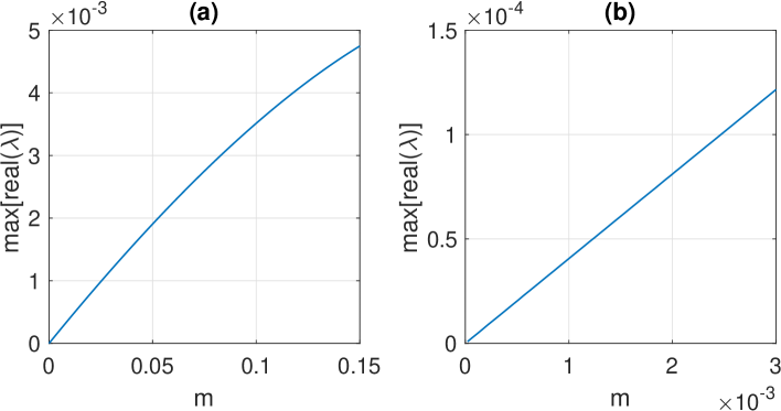
Figure 7: (a): Maximum of the real parts of the eigenvalues of the linearisation about a steady state of (39)-(40), (31) and (37), as a function of $m$. (b): Zoom of panel (a). Other parameters: $\mu=0.6,\nu=0.4,\alpha=\pi/2-0.05,D=10^{-13}$.

Olmi olm15 considered (24)-(25) for $\omega=1,N=200,\alpha=\pi/2-0.02$, and the same values of $\mu$ and $\nu$ as used here. Repeating the analysis above for this value of $\alpha$ we find qualitatively the same picture as that shown in Fig. 7. Olmi observed that even for $m=10^{-4}$, oscillations in the magnitude of the order parameter of the asynchronous population grew, “but over very long times scales,” consistent with our results. Repeating the calculations shown in Fig. 7 but for $\alpha=\pi/2-0.02$, then interpolating to find the real part of the rightmost eigenvalues for $m=10^{-4}$, we obtain $\sim 4.8\times 10^{-6}$. Thus over $5\times 10^{5}$ time units, we expect the amplitude of these fluctuations to grow by a factor of approximately $\exp{(4.8\times 10^{-6}\times 5\times 10^{5})}\approx 11$, in excellent agreement with Olmi’s observation of growth by a factor of $10$.

In conclusion, stable chimera states (stationary in a uniformly rotating frame) do not exist in (24)-(25) for infinite $N$ for any small values of $m$ using the values of other parameters from boukan14 , or from olm15 .

II.3 FitzHugh-Nagumo oscillators

In this section we consider two populations of FitzHugh-Nagumo oscillators. In omeome13 the authors considered a ring of such oscillators, nonlocally coupled, and showed numerically that such a system could support chimeras.

Consider the following network:

$$\epsilon\frac{du_{i}}{dt} =u_{i}-u_{i}^{3}/3-v_{i}+\mu\left[b_{uu}\left(U_{1}-u_{i}\right)+b_{uv}\left(V_{1}-v_{i}\right)\right]$$

$$+\nu\left[b_{uu}\left(U_{2}-u_{i}\right)+b_{uv}\left(V_{2}-v_{i}\right)\right]$$ (42)

$$\frac{dv_{i}}{dt} =u_{i}+a+\mu\left[b_{vu}\left(U_{1}-u_{i}\right)+b_{vv}\left(V_{1}-v_{i}\right)\right]+\nu\left[b_{vu}\left(U_{2}-u_{i}\right)+b_{vv}\left(V_{2}-v_{i}\right)\right]$$ (43)

for $i=1,2\dots N$ and

$$\epsilon\frac{du_{i}}{dt} =u_{i}-u_{i}^{3}/3-v_{i}+\mu\left[b_{uu}\left(U_{2}-u_{i}\right)+b_{uv}\left(V_{2}-v_{i}\right)\right]$$

$$+\nu\left[b_{uu}\left(U_{1}-u_{i}\right)+b_{uv}\left(V_{1}-v_{i}\right)\right]$$ (44)

$$\frac{dv_{i}}{dt} =u_{i}+a+\mu\left[b_{vu}\left(U_{2}-u_{i}\right)+b_{vv}\left(V_{2}-v_{i}\right)\right]+\nu\left[b_{vu}\left(U_{1}-u_{i}\right)+b_{vv}\left(V_{1}-v_{i}\right)\right]$$ (45)

for $i=N+1,\dots 2N$, where

$$U_{1}\equiv\frac{1}{N}\sum_{i=1}^{N}u_{i};\qquad V_{1}\equiv\frac{1}{N}\sum_{i=1}^{N}v_{i}$$ (46)

and

$$\qquad U_{2}\equiv\frac{1}{N}\sum_{i=1}^{N}u_{N+i};\qquad V_{2}\equiv\frac{1}{N}\sum_{i=1}^{N}v_{N+i}$$ (47)

We have

$$\begin{pmatrix}b_{uu}&b_{uv}\\ b_{vu}&b_{vv}\end{pmatrix}=\begin{pmatrix}\cos{\phi}&\sin{\phi}\\ -\sin{\phi}&\cos{\phi}\end{pmatrix}$$ (48)

for some phase $\phi$. Coupling within each population has strength $\mu$ and that between populations has strength $\nu$, and we control their relative strength by defining $\mu=(1+A)/20$ and $\nu=(1-A)/20$. Numerically, we find a stable chimera state for $\phi=\pi/2-0.1,\epsilon=0.1,a=0.5,A=0.2$, as shown in Fig. 8. Since $\epsilon$ is small the oscillators are relaxation oscillators, with strongly nonlinear waveforms.

Since each oscillator rotates around the origin, we can define an average angular velocity by counting the number of rotations each one makes during a long time interval and dividing by the duration of that interval omeome13 . Doing so we find that for these parameter values the asynchronous group has average angular velocity $\omega=2.1516$ while the synchronous group has $\omega=2.0511$. While these values are close, the fact that they are different shows that this is a chimera state.

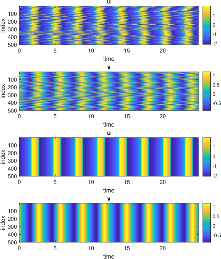
Figure 8: A chimera state for equations (42)-(45). The top two rows show $u$ and $v$ for population one, and the bottom two show them for population two. Parameters: $N=500,\phi=\pi/2-0.1,\epsilon=0.1,a=0.5,A=0.2$.

Suppose population two is synchronised. Its dynamics is described by

$$\epsilon\frac{dU_{2}}{dt} =U_{2}-U_{2}^{3}/3-V_{2}+\nu\left[b_{uu}\left(U_{1}-U_{2}\right)+b_{uv}\left(V_{1}-V_{2}\right)\right]$$ (49)

$$\frac{dV_{2}}{dt} =U_{2}+a+\nu\left[b_{vu}\left(U_{1}-U_{2}\right)+b_{vv}\left(V_{1}-V_{2}\right)\right]$$ (50)

In population one we have

$$\epsilon\frac{du_{i}}{dt} =u_{i}-u_{i}^{3}/3-v_{i}+\mu\left[b_{uu}\left(U_{1}-u_{i}\right)+b_{uv}\left(V_{1}-v_{i}\right)\right]$$

$$+\nu\left[b_{uu}\left(U_{2}-u_{i}\right)+b_{uv}\left(V_{2}-v_{i}\right)\right]$$ (51)

$$\frac{dv_{i}}{dt} =u_{i}+a+\mu\left[b_{vu}\left(U_{1}-u_{i}\right)+b_{vv}\left(V_{1}-v_{i}\right)\right]$$

$$+\nu\left[b_{vu}\left(U_{2}-u_{i}\right)+b_{vv}\left(V_{2}-v_{i}\right)\right]$$ (52)

for $i=1,2\dots N$. Writing $r_{i}^{2}=u_{i}^{2}+v_{i}^{2}$ and $\tan{\theta_{i}}=v_{i}/u_{i}$ so that $u_{i}=r_{i}\cos{\theta_{i}}$ and $v_{i}=r_{i}\sin{\theta_{i}}$ we have

$$\frac{dr_{i}}{dt} =\frac{u_{i}\frac{du_{i}}{dt}+v_{i}\frac{dv_{i}}{dt}}{r_{i}}\equiv F(r_{i},\theta_{i},U_{1},V_{1},U_{2},V_{2})$$ (53)

$$\frac{d\theta_{i}}{dt} =\frac{u_{i}\frac{dv_{i}}{dt}-v_{i}\frac{du_{i}}{dt}}{r_{i}^{2}}\equiv G(r_{i},\theta_{i},U_{1},V_{1},U_{2},V_{2})$$ (54)

Thus we consider the dynamical system

$$\frac{\partial R}{\partial t}(\theta,t) =F(R,\theta,U_{1},V_{1},U_{2},V_{2})-G(R,\theta,U_{1},V_{1},U_{2},V_{2})\frac{\partial R}{\partial\theta}+D\frac{\partial^{2}}{\partial\theta^{2}}R(\theta,t)$$ (55)

$$\frac{\partial P}{\partial t}(\theta,t) =-\frac{\partial}{\partial\theta}\left[P(\theta,t)G(R,\theta,U_{1},V_{1},U_{2},V_{2})\right]+D\frac{\partial^{2}}{\partial\theta^{2}}P(\theta,t)$$ (56)

together with (49)-(50), where

$$U_{1}=\int_{0}^{2\pi}P(\theta,t)R(\theta,t)\cos{\theta}d\theta$$ (57)

and

$$V_{1}=\int_{0}^{2\pi}P(\theta,t)R(\theta,t)\sin{\theta}d\theta$$ (58)

and we have added a small amount of diffusion in both (55)-(56) to stabilise solutions. A significant difference between the system studied in this section and those in Secs. II.1 and II.2 (and II.4, below) is that the FitzHugh-Nagumo system is not invariant under a global phase shift. Thus the chimera state of interest is a stable periodic solution of (55)-(56) and (49)-(50), as seen in Fig. 9.

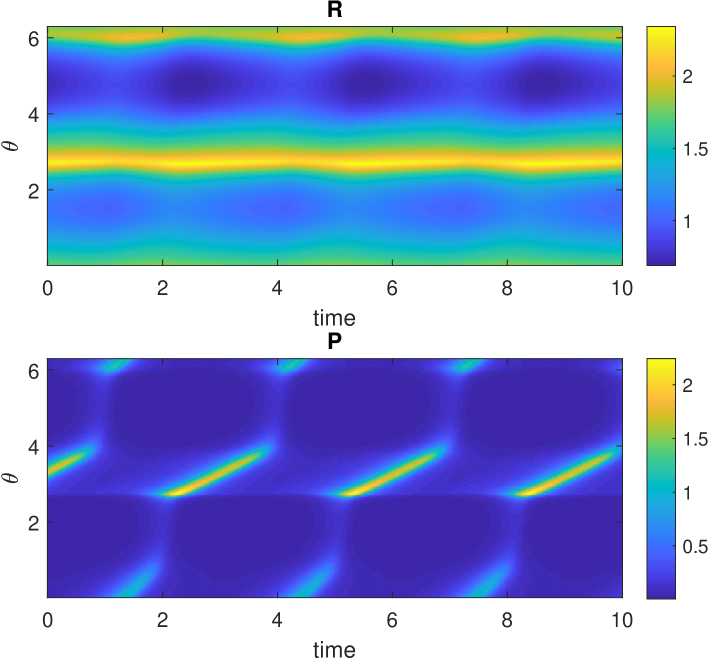
Figure 9: A chimera state for equations (55)-(56) and (49)-(50). The top row shows $R(\theta,t)$ and the bottom one $P(\theta,t)$. Parameters: $\phi=\pi/2-0.1,\epsilon=0.1,a=0.5,A=0.2,D=10^{-3}$. ($\theta$ is discretised with 256 points.)

Performing numerical continuation of this periodic orbit in $A$ we find that it undergoes a Hopf bifurcation as $A$ is increased, as shown in Fig. 10. Numerical simulation indicates that this is a supercritical bifurcation. Decreasing $D$ decreases the value of $A$ at which the Hopf bifurcation occurs, suggesting that the “true” bifurcation occurs at a lower value than that shown in Fig. 10. Indeed, simulations of (42)-(45) with $N=5000$ show that the Hopf bifurcation occurs at some $A\in(0.25,0.3)$.

(To perform numerical continuation of the periodic orbit we define a Poincaré section at $V_{2}=0,\dot{V_{2}}>0$ and integrate (55)-(56) and (49)-(50) from an initial condition on this section until the system hits the section for the first time. This defines a map in all other variables from the section to itself, and a fixed point of this map is the periodic orbit of interest. Linearising the map about the fixed point gives the Floquet multipliers and hence stability of the periodic orbit.)

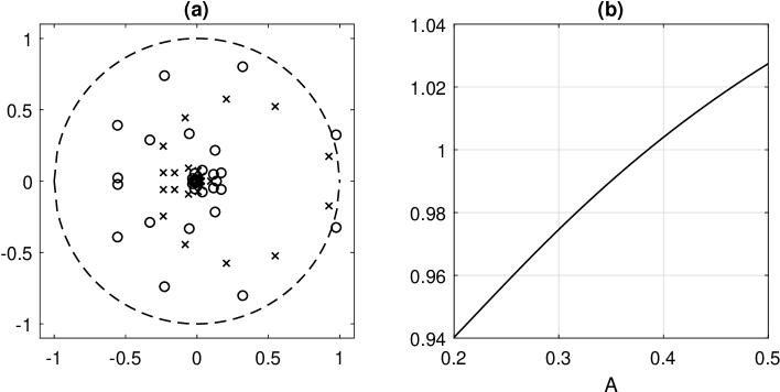
Figure 10: Hopf bifurcation of a periodic solution of (55)-(56) and (49)-(50). (a): Floquet multipliers of the periodic orbit at $A=0.2$ (crosses) and $A=0.5$ (circles). The unit circle is shown dashed. (b): maximum of the magnitude of the Floquet multipliers as a function of $A$. Parameters: $\phi=\pi/2-0.1,\epsilon=0.1,a=0.5,D=10^{-3}$. ($\theta$ is discretised with 256 points.)

If we solve (55)-(56) and (49)-(50) with (57)-(58) as drivers for

$$\epsilon\frac{du}{dt} =u-u^{3}/3-v+\mu\left[b_{uu}\left(U_{1}-u\right)+b_{uv}\left(V_{1}-v\right)\right]$$

$$+\nu\left[b_{uu}\left(U_{2}-u_{i}\right)+b_{uv}\left(V_{2}-v_{i}\right)\right]$$ (59)

$$\frac{dv}{dt} =u+a+\mu\left[b_{vu}\left(U_{1}-u\right)+b_{vv}\left(V_{1}-v\right)\right]+\nu\left[b_{vu}\left(U_{2}-u\right)+b_{vv}\left(V_{2}-v\right)\right]$$ (60)

governing the dynamics of a single oscillator in the incoherent population, we find that $u$ and $v$ follow a stable quasiperiodic orbit, as shown in Fig. 11, with mean rotation frequency $\omega=2.1553$ while the synchronous group (i.e. $U_{2}$ and $V_{2}$) are periodic (as expected) with $\omega=2.0519$. These match quite well with the results from simulating a finite network (Fig. 8) and differences could be due to the finite $N$ used in Fig. 8 and the non-zero value of $D$ needed to stabilise the solutions of (55)-(56) and (49)-(50) ($D=10^{-3}$).

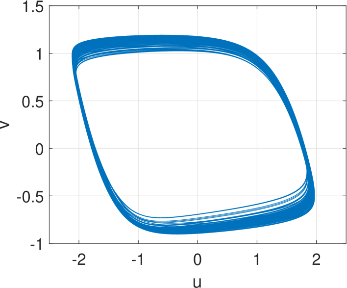
Figure 11: Dynamics of (59)-(60) driven by (55)-(56) and (49)-(50). Parameters: $A=0.2,\phi=\pi/2-0.1,\epsilon=0.1,a=0.5,D=10^{-3}$. (Discretised with 256 points.)

II.3.1 Alternating chimera

For a network formed from two populations, an alternating chimera may exist. In this state neither population is pefectly synchronised and the level of synchrony within each population varies periodically, but in antiphase to that of the other population hausch15 . One way that such a state can form is that under parameter variation, two coexisting “breathing” chimeras, in which one population is synchronised and the other is not (which are mapped to one another under relabelling of the populations), merge in a gluing bifurcation, resulting in an attractor which is invariant under relabelling of the populations lai12 .

Such a state occurs in (42)-(45) for $A=0.6$, i.e. after the Hopf bifurcation. Since oscillators in both populations now lie on (different) closed curves, we can write the dynamics for each curve. The equations governing the system are

$$\frac{\partial R_{1}}{\partial t}(\theta,t) =F(R_{1},\theta,U_{1},V_{1},U_{2},V_{2})-G(R_{1},\theta,U_{1},V_{1},U_{2},V_{2})\frac{\partial R_{1}}{\partial\theta}+D\frac{\partial^{2}}{\partial\theta^{2}}R_{1}(\theta,t)$$ (61)

$$\frac{\partial P_{1}}{\partial t}(\theta,t) =-\frac{\partial}{\partial\theta}\left[P_{1}(\theta,t)G(R_{1},\theta,U_{1},V_{1},U_{2},V_{2})\right]+D\frac{\partial^{2}}{\partial\theta^{2}}P_{1}(\theta,t)$$ (62)

and

$$\frac{\partial R_{2}}{\partial t}(\theta,t) =F(R_{2},\theta,U_{2},V_{2},U_{1},V_{1})-G(R_{2},\theta,U_{2},V_{2},U_{1},V_{1})\frac{\partial R_{2}}{\partial\theta}+D\frac{\partial^{2}}{\partial\theta^{2}}R_{2}(\theta,t)$$ (63)

$$\frac{\partial P_{2}}{\partial t}(\theta,t) =-\frac{\partial}{\partial\theta}\left[P_{2}(\theta,t)G(R_{2},\theta,U_{2},V_{2},U_{1},V_{1})\right]+D\frac{\partial^{2}P_{2}(\theta,t)}{\partial\theta^{2}}$$ (64)

where

$$U_{j}=\int_{0}^{2\pi}P_{j}(\theta,t)R_{j}(\theta,t)\cos{\theta}d\theta$$ (65)

and

$$V_{j}=\int_{0}^{2\pi}P_{j}(\theta,t)R_{j}(\theta,t)\sin{\theta}d\theta$$ (66)

To quantify the behaviour we define order parameters $Z_{j}=U_{j}+iV_{j}$ and plot the magnitude of both of these in the top two panels of Fig. 12. To compare with the behaviour of (42)-(45) we define

$$Z_{1}=\frac{1}{N}\sum_{k=1}^{N}u_{k}+\frac{i}{N}\sum_{k=1}^{N}v_{k}$$ (67)

and

$$Z_{2}=\frac{1}{N}\sum_{k=1}^{N}u_{N+k}+\frac{i}{N}\sum_{k=1}^{N}v_{N+k}$$ (68)

and plot their magnitudes in the bottom two panels of Fig. 12 for $N=500$. We see alternations, as expected, and the range of values and the form of oscillations is correct. The main difference between the two systems is the timescale of alternation. This is probably due to the finite size of the population in (42)-(45), the non-zero value of $D$ used in (61)-(64), and presumed closeness to a gluing bifurcation, in which two symmetrically related breathing chimeras merge to form the alternating chimera, as in lai12 . Since this bifurcation involves a quasiperiodic orbit approaching a saddle periodic orbit, we expect that the time it spends near the saddle orbit, and thus the period of the slow oscillations seen in Fig. 12, to be quite sensitive to the differences between the two systems being studied here.

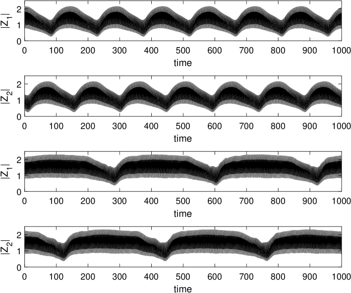
Figure 12: An alternating chimera state. Top two panels: magnitudes of the order parameters defined for (61)-(64) (discretised in $\theta$ using 256 points, $D=10^{-4}$.). Bottom two panels: magnitudes of the order parameters defined for (42)-(45) (with $N=500$). Parameters: $A=0.6,\phi=\pi/2-0.1,\epsilon=0.1,a=0.5$.

II.4 Delay

Chimeras have been studied in a number of systems with delays omemai08 ; setsen08 ; lai09 . In this section we consider the system

$$\frac{dX_{j}(t)}{dt} =i\omega X_{j}(t)+\gamma(1-|X_{j}(t)|^{2})X_{j}(t)+\frac{\mu}{N}\sum_{k=1}^{N}X_{k}(t-\tau_{1})+\frac{\nu}{N}\sum_{k=1}^{N}X_{N+k}(t-\tau_{2})$$ (69)

for $j=1,\dots N$ and

$$\frac{dX_{j}(t)}{dt} =i\omega X_{j}(t)+\gamma(1-|X_{j}(t)|^{2})X_{j}(t)+\frac{\mu}{N}\sum_{k=1}^{N}X_{N+k}(t-\tau_{1})+\frac{\nu}{N}\sum_{k=1}^{N}X_{k}(t-\tau_{2})$$ (70)

for $j=N+1,\dots 2N$, where each $X_{j}\in\mathbb{C}$, i.e. two populations of Stuart-Landau oscillators with coupling within a population of strength $\mu$, delayed by $\tau_{1}$, and coupling between populations of strength $\nu$, delayed by $\tau_{2}$. We find that there is a chimera for parameters $\omega=3,\gamma=10,\mu=0.36,\nu=0.04,\tau_{1}=0.6,\tau_{2}=0.4$, in a system with $N=100$ (not shown). The asynchronous group has an average angular frequency of $2.9871$, and the synchronised group has angular frequency $2.6348$.

Suppose population two is synchronised. Then its dynamics is described by

$$\frac{dX(t)}{dt}=i\omega X(t)+\gamma(1-|X(t)|^{2})X(t)+\mu X(t-\tau_{1})+\nu Z(t-\tau_{2})$$ (71)

where

$$Z(t)=\frac{1}{N}\sum_{k=1}^{N}X_{k}(t)$$ (72)

In population one we have

$$\frac{dX_{j}(t)}{dt} =i\omega X_{j}(t)+\gamma(1-|X_{j}(t)|^{2})X_{j}(t)+\mu Z(t-\tau_{1})+\nu X(t-\tau_{2})$$ (73)

for $j=1,\dots N$. Writing $X_{j}=r_{j}e^{i\theta_{j}}$ we have

$$\frac{dr_{j}}{dt} =\gamma[1-r_{j}^{2}(t)]r_{j}(t)+\mbox{Re}\left\{[\mu Z(t-\tau_{1})+\nu X(t-\tau_{2})]e^{-i\theta_{j}(t)}\right\}$$

$$\equiv F[r_{j}(t),\theta_{j}(t),Z(t-\tau_{1}),X(t-\tau_{2})]$$ (74)

$$\frac{d\theta_{j}}{dt} =\omega+\mbox{Im}\left\{[\mu Z(t-\tau_{1})+\nu X(t-\tau_{2})]e^{-i\theta_{j}}(t)\right\}/r_{j}(t)$$

$$\equiv G[r_{j}(t),\theta_{j}(t),Z(t-\tau_{1}),X(t-\tau_{2})]$$ (75)

Thus we consider the dynamical system

$$\frac{\partial R}{\partial t}(\theta,t) =F[R(\theta,t),\theta,Z(t-\tau_{1}),X(t-\tau_{2})]$$

$$-G[R(\theta,t),\theta,Z(t-\tau_{1}),X(t-\tau_{2})]\frac{\partial R}{\partial\theta}(\theta,t)$$ (76)

$$\frac{\partial P}{\partial t}(\theta,t) =-\frac{\partial}{\partial\theta}\left\{P(\theta,t)G[R(\theta,t),\theta,Z(t-\tau_{1}),X(t-\tau_{2})]\right\}+D\frac{\partial^{2}}{\partial\theta^{2}}P(\theta,t)$$ (77)

together with (71) where

$$Z(t)=\int_{0}^{2\pi}P(\theta,t)R(\theta,t)e^{i\theta}d\theta$$ (78)

We set the level of diffusion to be $D=10^{-6}$.

This system is invariant under rotation in the complex plane of each $X_{j}$ by the same angle so we can go to a rotating coordinate frame in which the chimera is stationary. In this frame, defining $\tilde{X}(t)=X(t)e^{-i\Omega t}$ and $\tilde{Z}(t)=Z(t)e^{-i\Omega t}$ we find that $\tilde{X}$ satisfies

$$\frac{d\tilde{X}(t)}{dt} =i(\omega-\Omega)\tilde{X}(t)+\gamma(1-|\tilde{X}(t)|^{2})\tilde{X}(t)+\mu\tilde{X}(t-\tau_{1})e^{-i\Omega\tau_{1}}+\nu\tilde{Z}(t-\tau_{2})e^{-i\Omega\tau_{2}}$$ (79)

where $\Omega$ is the speed of rotation. Note that moving to a rotating frame causes effective phase shifts in $\tilde{X}$ and $\tilde{Z}$. Writing $\tilde{X}_{j}(t)=X_{j}(t)e^{-i\Omega t}=\tilde{r}_{j}(t)e^{i\tilde{\theta}_{j}(t)}$ we find that in population one,

$$\frac{d\tilde{r}_{j}}{dt} =\gamma[1-\tilde{r}_{j}^{2}(t)]\tilde{r}_{j}(t)+\mbox{Re}\left\{[\mu\tilde{Z}(t-\tau_{1})e^{-i\Omega\tau_{1}}+\nu\tilde{X}(t-\tau_{2})e^{-i\Omega\tau_{2}}]e^{-i\tilde{\theta}_{j}(t)}\right\}$$

$$\equiv\tilde{F}[\tilde{r}_{j}(t),\tilde{\theta}_{j}(t),\tilde{Z}(t-\tau_{1}),\tilde{X}(t-\tau_{2})]$$ (80)

$$\frac{d\tilde{\theta}_{j}}{dt} =\omega-\Omega+\mbox{Im}\left\{[\mu\tilde{Z}(t-\tau_{1})e^{-i\Omega\tau_{1}}+\nu\tilde{X}(t-\tau_{2})e^{-i\Omega\tau_{2}}]e^{-i\tilde{\theta}_{j}(t)}\right\}/\tilde{r}_{j}(t)$$

$$\equiv\tilde{G}[\tilde{r}_{j}(t),\tilde{\theta}_{j}(t),\tilde{Z}(t-\tau_{1}),\tilde{X}(t-\tau_{2})]$$ (81)

We are thus interested in steady states of

$$\frac{\partial R}{\partial t}(\theta,t) =\tilde{F}[R(\theta,t),\theta,\tilde{Z}(t-\tau_{1}),\tilde{X}(t-\tau_{2})]$$

$$-\tilde{G}[R(\theta,t),\theta,\tilde{Z}(t-\tau_{1}),\tilde{X}(t-\tau_{2})]\frac{\partial R}{\partial\theta}(\theta,t)$$ (82)

$$\frac{\partial P}{\partial t}(\theta,t) =-\frac{\partial}{\partial\theta}\left\{P(\theta,t)\tilde{G}[R(\theta,t),\theta,\tilde{Z}(t-\tau_{1}),\tilde{X}(t-\tau_{2})]\right\}+D\frac{\partial^{2}}{\partial\theta^{2}}P(\theta,t)$$ (83)

along with (79) where

$$\tilde{Z}(t)=\int_{0}^{2\pi}P(\theta,t)R(\theta,t)e^{i\theta}d\theta$$ (84)

Such a steady state is shown in Fig. 13, where $\Omega=2.6375$. (Matlab’s dde23 routine was used for time integration.) Numerical study of delay differential equations is significantly more difficult than that of non-delayed equations, so we discretise $\theta$ in only 32 equally spaced points. As can be seen in Fig. 13 the solutions are quite smooth functions of $\theta$, and spatial derivatives are evaluated spectrally.

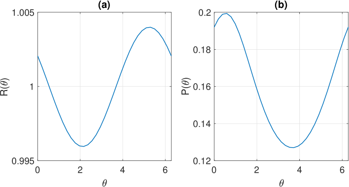
Figure 13: Steady state of (82)-(83) and (79). Parameters: $\omega=3,\gamma=10,\mu=0.36,\nu=0.04,\tau_{1}=0.6,\tau_{2}=0.4,D=10^{-6}$.

Having found the steady state of (82)-(83) and (79) we can numerically integrate the ODEs

$$\frac{dr}{dt}=\tilde{F}[r,\theta,\tilde{Z},\tilde{X}];\qquad\frac{d\theta}{dt}=\tilde{G}[r,\theta,\tilde{Z},\tilde{X}]$$ (85)

where $\tilde{Z}$ and $\tilde{X}$ no longer depend on time, in order to find the period of an oscillator in the incoherent group relative to the frequency of the locked group ($\Omega$). For the parameters used here, (85) has a stable periodic orbit with angular frequency $\sim 0.35338$, showing that the coherent and incoherent groups do have different average frequencies, as expected for a chimera state. Adding this frequency to the measured value of $\Omega$ we obtain $2.9909$, in very good agreement with the measured angular frequency from the finite simulation ($2.9871$).

We can following the steady state shown in Fig. 13 as $\omega$ is decreased using the software DDE-BIFTOOL ddebif . Doing so we find that it becomes unstable through a subcritical Hopf bifurcation, as shown in Fig. 14. We can also follow the unstable periodic orbit created in this bifurcation as $\omega$ is varied. To represent the unstable periodic orbit we track the maximum over $\theta$ of $P(\theta,t)$, and then show the maximum and minimum values over one period of this, with open circles.

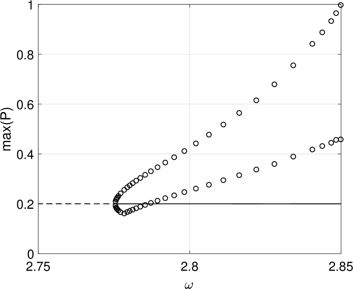
Figure 14: Lines: maximum of $P(\theta)$ at steady states of (82)-(83) and (79) (solid: stable; dashed: unstable). Open circles: unstable periodic orbit created in a subcritical Hopf bifurcation (see text). Parameters: $\gamma=10,\mu=0.36,\nu=0.04,\tau_{1}=0.6,\tau_{2}=0.4,D=10^{-6}$. (Discretised with 32 points.)

Increasing $\omega$ in the discrete network (69)-(70) to $\omega=3.2$ destabilises the chimera state, and the system moves to a state where both populations are incoherent, as shown in Fig. 15. Such an instability cannot be detected using the approach presented above, which assumes that one population is perfectly synchronised.

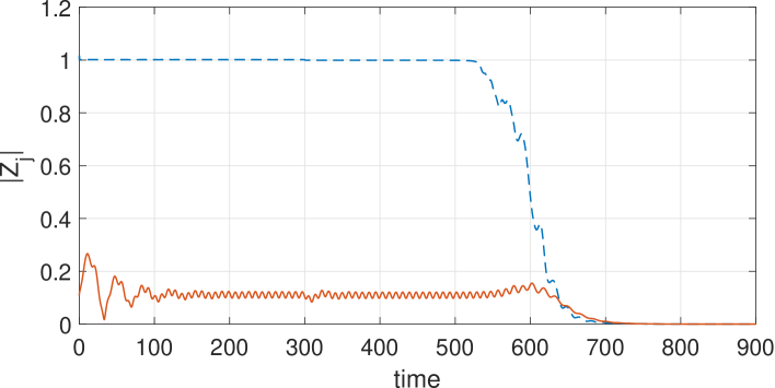
Figure 15: Solution of (69)-(70). $Z_{1}(t)\equiv N^{-1}\sum_{k=1}^{N}X_{k}(t)$ and $Z_{2}(t)\equiv N^{-1}\sum_{k=1}^{N}X_{N+k}(t)$. $\omega$ is increased from 3 to 3.2 at $t=300$. Parameters: $\gamma=10,\mu=0.36,\nu=0.04,\tau_{1}=0.6,\tau_{2}=0.4,N=100$.

III Discussion

We have used the results of clupol18 to study the dynamics of chimera states in networks formed from two populations of identical oscillators, with different strengths of coupling both within and between populations. We studied four different types of oscillators. In Sec. II.1 we revisited the system of Stuart-Landau oscillators studied in lai10 and put results that were inferred in that paper on a solid footing. In Sec. II.2 we consider Kuramoto oscillators with inertia, previously studied in boukan14 ; olm15 . We showed that stable stationary chimeras do not exist is such systems, at least for an infinite number of oscillators and for the parameter values previously considered. In Sec. II.3 we considered FitzHugh-Nagumo oscillators whose oscillations are highly nonlinear. This system is unlike the three others studied, as the oscillators are not invariant under a phase shift, and thus the chimera state of interest is actually a periodic orbit rather than a fixed point in a rotating coordinate frame. Lastly (Sec. II.4) we considered Stuart-Landau oscillators with delayed coupling. We have provided rigorous numerical results on the existence and stability of chimeras in these networks, in contrast to the many presentations showing results of only numerical simulations of finite networks of oscillators.

Regarding future work, all of the results presented here consider identical oscillators. However, at least for sinusoidally-coupled phase oscillators it is known that systems of identical oscillators have non-generic properties such as a large number of conserved quantities watstr94 , and making them heterogeneous removes this degeneracy lai09a ; ottant08 . To investigate this we numerically integrated (8)-(9), but having made the system heterogeneous by choosing the value of $\omega$ for each oscillator randomly and independently from a uniform distribution. A snapshot of the solution is shown in Fig. 16, where the oscillators are coloured by their $\omega$ value. This state can still be regarded as a chimera, as it is a small perturbation from the chimera that exists for identical oscillators. For both populations, the oscillators lie on a smooth curve. However, for the asynchronous population there seems to be no correspondence between the value of $\omega$ and an oscillator’s position on the curve, while in the nearly synchronous group the oscillators are clearly ordered by the value of $\omega$. It may be possible to derive a theory to cover this type of solution.

It would also be of interest to develop a theory for oscillators described by more than two variables, assuming that the incoherent oscillators still lie on a closed curve in phase space.

While we have considered abstract networks of oscillators, the modelling of neurons or groups of neurons by oscillators is common ashcoo16 . A network of two populations, as studied here, naturally arises when modelling the dynamics of competition between two competing percepts, for example in binocular rivalry laicho02 . The techniques presented here may be useful in further understanding the dynamics of such networks.

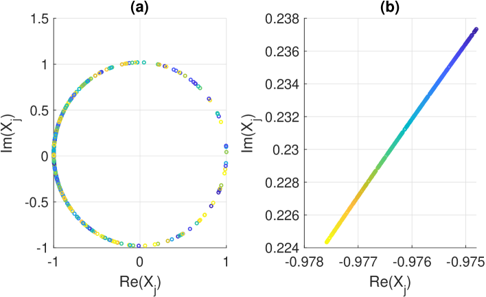
Figure 16: Snapshot of a solution of (8)-(9) where for each oscillator, $\omega$ was randomly chosen from a uniform distribution on $[0,0.002]$. (a): asynchronous population; (b): nearly synchronous population. Note the different scales. Colour indicates the value of each $\omega$. Parameters: $\epsilon=0.05,\beta=0.08,A=0.2,\delta=-0.1,N=500$.

References

- (1) Mark J Panaggio and Daniel M Abrams. Chimera states: coexistence of coherence and incoherence in networks of coupled oscillators. Nonlinearity, 28(3):R67, 2015.
- (2) O E Omel’chenko. The mathematics behind chimera states. Nonlinearity, 31(5):R121–R164, apr 2018.
- (3) Iryna Omelchenko, Oleh E. Omel’chenko, Philipp Hövel, and Eckehard Schöll. When nonlocal coupling between oscillators becomes stronger: Patched synchrony or multichimera states. Phys. Rev. Lett., 110:224101, May 2013.
- (4) Daniel M. Abrams and Steven H. Strogatz. Chimera states in a ring of nonlocally coupled oscillators. Int. J. Bifn. Chaos, 16:21–37, 2006.
- (5) Daniel M. Abrams and Steven H. Strogatz. Chimera states for coupled oscillators. Phys. Rev. Lett., 93:174102, 2004.
- (6) Y. Kuramoto and D. Battogtokh. Coexistence of Coherence and Incoherence in Nonlocally Coupled Phase Oscillators. Nonlinear Phenom. Complex Syst., 5:380–385, 2002.
- (7) Carlo R Laing. Chimeras in two-dimensional domains: heterogeneity and the continuum limit. SIAM Journal on Applied Dynamical Systems, 16(2):974–1014, 2017.
- (8) Oleh E Omel’chenko, Matthias Wolfrum, Serhiy Yanchuk, Yuri L Maistrenko, and Oleksandr Sudakov. Stationary patterns of coherence and incoherence in two-dimensional arrays of non-locally-coupled phase oscillators. Physical Review E, 85(3):036210, 2012.
- (9) Mark J Panaggio and Daniel M Abrams. Chimera states on the surface of a sphere. Physical Review E, 91(2):022909, 2015.
- (10) Jianbo Xie, Edgar Knobloch, and Hsien-Ching Kao. Twisted chimera states and multicore spiral chimera states on a two-dimensional torus. Physical Review E, 92(4):042921, 2015.
- (11) S. Shima and Y. Kuramoto. Rotating spiral waves with phase-randomized core in nonlocally coupled oscillators. Physical Review E, 69(3):036213, 2004.
- (12) Erik A Martens, Carlo R Laing, and Steven H Strogatz. Solvable model of spiral wave chimeras. Physical review letters, 104(4):044101, 2010.
- (13) Daniel M. Abrams, Rennie Mirollo, Steven H. Strogatz, and Daniel A. Wiley. Solvable model for chimera states of coupled oscillators. Phys. Rev. Lett., 101:084103, 2008.
- (14) Carlo R. Laing. Chimera states in heterogeneous networks. Chaos, 19:013113, 2009.
- (15) K Premalatha, VK Chandrasekar, M Senthilvelan, and M Lakshmanan. Chimeralike states in two distinct groups of identical populations of coupled stuart-landau oscillators. Physical Review E, 95(2):022208, 2017.
- (16) Erik A Martens, Christian Bick, and Mark J Panaggio. Chimera states in two populations with heterogeneous phase-lag. Chaos: An Interdisciplinary Journal of Nonlinear Science, 26(9):094819, 2016.
- (17) Mark J Panaggio, Daniel M Abrams, Peter Ashwin, and Carlo R Laing. Chimera states in networks of phase oscillators: the case of two small populations. Physical Review E, 93(1):012218, 2016.
- (18) Arkady Pikovsky and Michael Rosenblum. Partially integrable dynamics of hierarchical populations of coupled oscillators. Phys. Rev. Lett., 101:264103, 2008.
- (19) Mark R Tinsley, Simbarashe Nkomo, and Kenneth Showalter. Chimera and phase-cluster states in populations of coupled chemical oscillators. Nature Physics, 8(9):662, 2012.
- (20) Erik Andreas Martens, Shashi Thutupalli, Antoine Fourrière, and Oskar Hallatschek. Chimera states in mechanical oscillator networks. Proceedings of the National Academy of Sciences, 110(26):10563–10567, 2013.
- (21) Ernest Montbrió, Jürgen Kurths, and Bernd Blasius. Synchronization of two interacting populations of oscillators. Phys. Rev. E, 70:056125, 2004.
- (22) Pau Clusella and Antonio Politi. Between phase and amplitude oscillators. Phys. Rev. E, 99:062201, Jun 2019.
- (23) C. van Vreeswijk. Partial synchronization in populations of pulse-coupled oscillators. Phys. Rev. E, 54:5522–5537, Nov 1996.
- (24) Pau Clusella, Antonio Politi, and Michael Rosenblum. A minimal model of self-consistent partial synchrony. New Journal of Physics, 18(9):093037, 2016.
- (25) Andrea Vüllings, Johanne Hizanidis, Iryna Omelchenko, and Philipp Hövel. Clustered chimera states in systems of type-i excitability. New Journal of Physics, 16(12):123039, 2014.
- (26) Iryna Omelchenko, Anna Zakharova, Philipp Hövel, Julien Siebert, and Eckehard Schöll. Nonlinearity of local dynamics promotes multi-chimeras. Chaos: An Interdisciplinary Journal of Nonlinear Science, 25(8):083104, 2015.
- (27) Tassos Bountis, Vasileios G Kanas, Johanne Hizanidis, and Anastasios Bezerianos. Chimera states in a two–population network of coupled pendulum–like elements. The European Physical Journal Special Topics, 223(4):721–728, 2014.
- (28) Simona Olmi. Chimera states in coupled kuramoto oscillators with inertia. Chaos: An Interdisciplinary Journal of Nonlinear Science, 25(12):123125, 2015.
- (29) Igor V Belykh, Barrett N Brister, and Vladimir N Belykh. Bistability of patterns of synchrony in kuramoto oscillators with inertia. Chaos: An Interdisciplinary Journal of Nonlinear Science, 26(9):094822, 2016.
- (30) Carlo R Laing. Chimeras in networks of planar oscillators. Physical Review E, 81(6):066221, 2010.
- (31) Simona Olmi, Antonio Politi, and Alessandro Torcini. Collective chaos in pulse-coupled neural networks. EPL (Europhysics Letters), 92(6):60007, 2011.
- (32) Irmantas Ratas and Kestutis Pyragas. Symmetry breaking in two interacting populations of quadratic integrate-and-fire neurons. Phys. Rev. E, 96:042212, Oct 2017.
- (33) Edward Ott and Thomas M. Antonsen. Low dimensional behavior of large systems of globally coupled oscillators. Chaos, 18:037113, 2008.
- (34) C. Laing. The dynamics of chimera states in heterogeneous Kuramoto networks. Physica D, 2009.
- (35) Erik A Martens. Bistable chimera attractors on a triangular network of oscillator populations. Physical Review E, 82(1):016216, 2010.
- (36) S. Watanabe and SH Strogatz. Constants of motion for superconducting Josephson arrays. Physica. D, 74:197–253, 1994.
- (37) Lloyd N Trefethen. Spectral methods in MATLAB, volume 10. Siam, 2000.
- (38) Bard Ermentrout. Gap junctions destroy persistent states in excitatory networks. Physical Review E, 74(3):031918, 2006.
- (39) Carlo R. Laing. Numerical bifurcation theory for high-dimensional neural models. The Journal of Mathematical Neuroscience, 4(1):1–27, 2014.
- (40) E. Doedel, RC Paffenroth, AR Champneys, TF Fairgrieve, Y.A. Kuznetsov, B. Sandstede, and X. Wang. AUTO 2000: Continuation and Bifurcation Software for Ordinary Differential Equations (with HomCont). Concordia University, Canada, ftp. cs. concordia. ca/pub/doedel/auto.
- (41) Erik A Martens. Chimeras in a network of three oscillator populations with varying network topology. Chaos: An Interdisciplinary Journal of Nonlinear Science, 20(4):043122, 2010.
- (42) Sindre W Haugland, Lennart Schmidt, and Katharina Krischer. Self-organized alternating chimera states in oscillatory media. Scientific reports, 5:9883, 2015.
- (43) Carlo R Laing. Disorder-induced dynamics in a pair of coupled heterogeneous phase oscillator networks. Chaos, 22(4):043104, 2012.
- (44) O.E. Omel’chenko, Y.L. Maistrenko, and P.A. Tass. Chimera States: The Natural Link Between Coherence and Incoherence. Phys. Rev. Lett., 100:044105, 2008.
- (45) Gautam C Sethia, Abhijit Sen, and Fatihcan M Atay. Clustered chimera states in delay-coupled oscillator systems. Physical review letters, 100(14):144102, 2008.
- (46) Koen Engelborghs, Tatyana Luzyanina, and Dirk Roose. Numerical bifurcation analysis of delay differential equations using dde-biftool. ACM Transactions on Mathematical Software (TOMS), 28(1):1–21, 2002.
- (47) Peter Ashwin, Stephen Coombes, and Rachel Nicks. Mathematical frameworks for oscillatory network dynamics in neuroscience. The Journal of Mathematical Neuroscience, 6(1):2, 2016.
- (48) Carlo R Laing and Carson C Chow. A spiking neuron model for binocular rivalry. Journal of computational neuroscience, 12(1):39–53, 2002.