Leveraging External Knowledge for Out-Of-Vocabulary Entity Labeling

Abstract

Dealing with previously unseen slots is a challenging problem in a real-world multi-domain dialogue state tracking task. Other approaches rely on predefined mappings to generate candidate slot keys, as well as their associated values. This, however, may fail when the key, the value, or both, are not seen during training. To address this problem we introduce a neural network that leverages external knowledge bases (KBs) to better classify out-of-vocabulary slot keys and values. This network projects the slot into an attribute space derived from the KB, and, by leveraging similarities in this space, we propose candidate slot keys and values to the dialogue state tracker. We provide extensive experiments that demonstrate that our stratagem can improve upon a previous approach, which relies on predefined candidate mappings. In particular, we evaluate this approach by training a state-of-the-art model with candidates generated from our network, and obtained relative increases of 57.7% and 82.7% in F1 score and accuracy, respectively, for the aforementioned model, when compared to the current candidate generation strategy.

1 Introduction

In the Dialogue State Tracking task, the Slot Carryover (SC) paradigm Naik et al. (2018) involves tracking a key-value pair (a slot) throughout the dialogue. At every turn, a decision is made to whether to carry the slot over to the next turn. The values that each slot can take are established a priori in a hierarchical schema where the slot’s value has a key assigned to it, which is itself associated with a domain. This is used to generate the candidates to be tracked, but slot-to-slot mappings can be challenging, as the keys and values could have been unseen during training Xu and Hu (2018).

Domain	Slot Value	Slot Key
Weather	Boston	City_Weather
Search	Boston	Search_Location

Table 1: An example of a cross-domain slot. Note that there is no semantic difference in the word “Boston” across domains–“Boston” is a city–and is only a change in naming conventions.

This mapping relies on context to resolve ambiguity from values and keys. When a slot is mapped across domains, the given key is translated to its new representation on the target domain. See table Table 1 for an example. Two insights can be taken from this: first, the meaning of the key is preserved, and is only a change in naming conventions. Second, the key-value relationship could be seen–loosely speaking–as a type of hypernymic property. These semantic properties, along with the challenge presented by out-of-vocabulary (OOV) keys and values, motivates our work on this paper.

We surmise that it is possible to leverage knowledge bases (KBs) to build a model which automates the slot candidate generation, and circumvents the OOV problem. Our model collects several prospects, and determines the closest match with respect to the given context. We do not make assumptions about the geometry of the input spaces, and we opt instead to learn the metric as a secondary task, through the polynomial approximation to a Bregman divergence Banerjee et al. (2005).

Previous work exists on inferring labels with little to no information provided during training, such as zero and few-shot learning methods Snell et al. (2017), and hybrid approaches such as in Akata et al. (2013); Yogatama et al. (2015); Shi et al. (2018). Leveraging the hierarchical nature of a corpus is not a new approach either, as hypernym classification requires some sort of hierarchical assumption, for example, Murty et al. (2018); Fu et al. (2014); Nickel and Kiela (2017). Work has also been made on employing KBs to improve learning, as in Lee et al. (2015); Yang and Mitchell (2017). Finally, Bregman-based methods have garnered popularity as both a metric and a learning algorithm. A good example is the work of Banerjee et al., Banerjee et al. (2005) on clustering with Bregman divergences.

Our work is unique in its approach: it relies on a KB, but places emphasis on the hierarchy of the corpus to learn and measure distances. It leverages hypernyms as an implicitly hierarchical slot key namespace. It is important to note, however, that our problem is unrelated to the hypernym classification task.

The three contributions of this paper are: first, a model that is able to output slot candidates for a dialogue state tracker (DST), even when the slot’s value, key, or both, are OOV. This is done by leveraging KBs to learn the key’s attributes. Second, a method to approximate a generalized, hierarchical distance function–the Bregman divergence–without making assumptions about the geometry of the space we are working on. Third, an analysis of the performance of a DST in OOV contexts, under both its current hardcoded mappings, and our model. Our approach increases the performance of the DST by 26.01% and 51.08% in $F_{1}$ and accuracy, respectively, under 100% OOV settings.

We start out by describing our model in Section 2, and then, in Section 3, we present the results obtained from the evaluation of a DST with the candidates generated by our approach. We conclude in Section 4 with a discussion of our work.

2 Model

Figure 1: Architecture of our model. It computes the closest key $h_{i}\in\mathcal{H}$ for a slot value $w$, given a context $\mathcal{C}$ and a feature tensor $\mathcal{F}$. Both $\mathcal{F}$ and $\mathcal{H}$ are constructed by looking up $w$ in a set of KBs. The key-value pair is then passed in to SC for evaluation.

We aim to learn a conditional probability distribution $P(w\in h_{i}|\mathcal{C},\mathcal{F})$ which models the closest representative slot key $h_{i}\in\mathcal{H}$ for a slot value $w$ given both a context $\mathcal{C}$, and the set of possible features for all slot keys $\mathcal{F}$. As a secondary objective, we set the constraint that our definition of “closeness” will be relative to a learned distance $D$.

Let $w$ be a slot value to be classified. We first construct its feature tensor $\mathcal{F}$ by performing a lookup of $w$ on a set of semantically disjoint KBs, $\mathcal{K}$, such that each $\mathcal{F}_{ijk}\in\mathcal{F}$ is the $k^{th}$ set of related, yet not defining, terms to $w$, corresponding to the $j^{th}$ entry of $KB_{i}\in\mathcal{K}$. The assumption here is that a word is a collection of specific linguistic features Brinton (2000) and realized by its context Mikolov et al. (2013). We limit the results from each $KB_{i}$ to $n$ entries, sorted by a relevance metric inherent to each $KB_{i}$, e.g., number of playbacks in $KB_{\text{songs}}$.

As a brief example, let $w=$ “Clint Eastwood” and our KB set $\mathcal{K}=\{KB_{\text{Personalities}}\}$. $\mathcal{F}$ is then composed of a single set $\mathcal{F}_{\text{{personalities}}}=[\emph{actor},\emph{director},\emph{composer},\emph{mayor}]$. Each of these fields contain their own attributes, with their own corresponding values, such as $\mathcal{F}_{\text{{personalities}},\emph{mayor},\text{location}}=$ “Camel-by-the-Sea, CA”.

We then obtain the key tensor, $\mathcal{H}$, by performing a reverse traversal of the Wordnet Miller (1995) hypernyms for the feature vectors, $\mathcal{H}_{i}\in\mathcal{H},\;\mathcal{H}_{i}=WordNet(\mathcal{F}_{ij})$. The traversal is constrained to return only the first $m$ antecessor nodes, and we prune out the repeated entries.

Finally, we generate the context vector $\mathcal{C}$, which is a flattened, tokenized version of the input context.

The three streams constructed ($\mathcal{F}$, $\mathcal{H}$, and $\mathcal{C}$) are flattened, embedded in GloVE Pennington et al. (2014), and fed into independent Bi-LSTM encoders Graves et al. (2013). The independence is needed due to the fact that their inputs are assumed to belong to different semantic spaces.

$$F =BiLSTM_{F}(\mathcal{F})$$ (1)

$$H =BiLSTM_{H}(\mathcal{H})$$

$$C =BiLSTM_{D}(\mathcal{C})$$

Then, we extract the relationship amongst each of the encodings by projecting them onto one another.

$$\pi_{F} =FH^{T}$$ (2)

$$\pi_{C} =CH^{T}$$

We split the projection matrices $\pi_{C}$ and $\pi_{F}$ in $|\mathcal{H}|$-sized chunks, each corresponding to one of the slot keys in the original key tensor, and evaluate the distance between $\pi_{F}$ and $\pi_{C}$.

Abstractly, the context is referring to a single entry in $\mathcal{F}$, and our goal is to find out which one is the closest in meaning. Hence, we require a way to measure it such that $\delta(\pi_{F},\pi_{C})\neq\delta(\pi_{C},\pi_{F})$ for some pseudometric $\delta$. Many functions could meet this requirement, but most of the more commonly used ones are instances of the Bregman divergence Banerjee et al. (2005). Choosing the right Bregman divergence for a given space is a complex problem, and is beyond the scope of this task. Therefore, we opt to learn it through a polynomial approximation of fixed degree $r$. For this, we construct a simple feed-forward neural network $P$ of depth $r$ and output size of $1$, with a $ReLU$ unit as the final activation layer Nair and Hinton (2010). Our final Bregman approximator module $B$ for some $x\in\pi_{C},y\in\pi_{F}$ is given by:

$$B(x,y)=P(x)-P(y)-\langle x-y,\psi(P,y,\epsilon)\rangle$$ (3)

Where $\psi(P,y,\epsilon)=\frac{P(x+\epsilon)-P(x-\epsilon)}{2\epsilon}$ is the symmetric difference quotient estimator for the first derivative of $P$, where $y$ is the point near which to estimate the function, and $\epsilon$ a step size.

We use $B$ to extract the distances of the context to the features with respect to their given hypernyms:

$$D=\{B(c_{i},f_{i}),c_{i}\in\pi_{C},f_{i}\in\pi_{F}\}$$ (4)

Finally, we pass in the distances into a softmax function $s(x)_{i}=\frac{e^{x_{i}}}{\Sigma_{j}x_{j}}$ to obtain their probablistic representation. Softmax was the preferred layer due to the fact that it tends to skew results in such a way that allow us to minimize the distance between the obtained and the expected probability distributions.

$$P(w\in h_{i}|\mathcal{C},\mathcal{F})=s(d_{i}),\;\;d_{i}\in D,h_{i}\in H$$ (5)

Due to the nature of our approach and the normalization from $s(x)_{i}$, there are many low-confidence distances that will add noise, and could be detrimental to our training goal. To mitigate this, we implement a learnable threshold $\tau$ that allows us to prune out results:

$$P_{\tau}(w\in h_{i}|\mathcal{C},\mathcal{F})\left\{\begin{array}[]{ll}1&s(d_{i})\geq\tau\\ 0&else\\ \end{array}\right.$$ (6)

2.1 Training

During training, our input is of the form $(w,\mathcal{C},\ell)$, where $w$ is the input slot value, along with its context $\mathcal{C}$ and an expected slot key $\ell$, which is just an indicator to disambiguate $w$.

We minimize a loss function $\mathcal{L}(y,\hat{y})$ between our predictions $y=\{P(w\in h_{i}|\mathcal{C},\mathcal{F})|h_{i}\in\mathcal{H}\}$ and our expected clusters $\hat{y}$. We construct $\hat{y}$ dynamically, by performing a fuzzy search of $\ell$ in the key tensor, indexing it, and then normalizing it: $\hat{y}=\{\hat{h_{i}}|\hat{h_{i}}=\frac{1}{|\mathcal{H}|}\mathbf{1}_{\ell}(h_{i})\}$. The loss function is the KL divergence between our distributions:

$$\mathcal{L}(y,\hat{y})=-\Sigma_{i}\hat{y}_{i}log(\frac{\hat{y_{i}}}{y_{i}})$$ (7)

Strategy	${F_{1}}$ OOV (0%)	Accuracy OOV (0%)	${F_{1}}$ OOV (100%)	Accuracy OOV (100%)
HM	87.10	95.12	32.21	31.57
MLP	86.77	94.96	32.21	31.57
Our approach	73.75	90.43	58.32	82.65

Table 2: $F_{1}$ and accuracy results for SC under different OOV settings and candidate generation strategies.

2.2 Slot Carryover

We construct the candidates for the DST as follows: given a set of slot values $W$, we construct another set of slot candidates $\{(w_{j},\text{argmax}_{h_{i}}P(w_{j}\in h_{i}|\mathcal{C},\mathcal{F})),w_{j}\in W\}$. This last set is then used to train the tracker.

3 Evaluation

3.1 Candidate generation

Our experiments are conducted on a subset of data collected from a commercial voice assistant. We train and evaluate the SC model under three candidate generation strategies:

• Hardcoded maps (HM): The current implementation, which relies on a hand-written, cross-domain, mapping between the keys and their domains to generate slot candidates.

• Multilayer perceptron (MLP): The MLP (Figure 2) provides a baseline on the performance of models that do not use KBs. It is trained and evaluated on all the maps from HM, and outputs whether a given map is correct. It achieves 99.99% test accuracy.

• Our approach: Our approach constructs a slot candidate for a given context and value. We purposely use a much smaller dataset (about 5% the size of the data for HM) to train our model, to emphasize the zero-shot conditions.

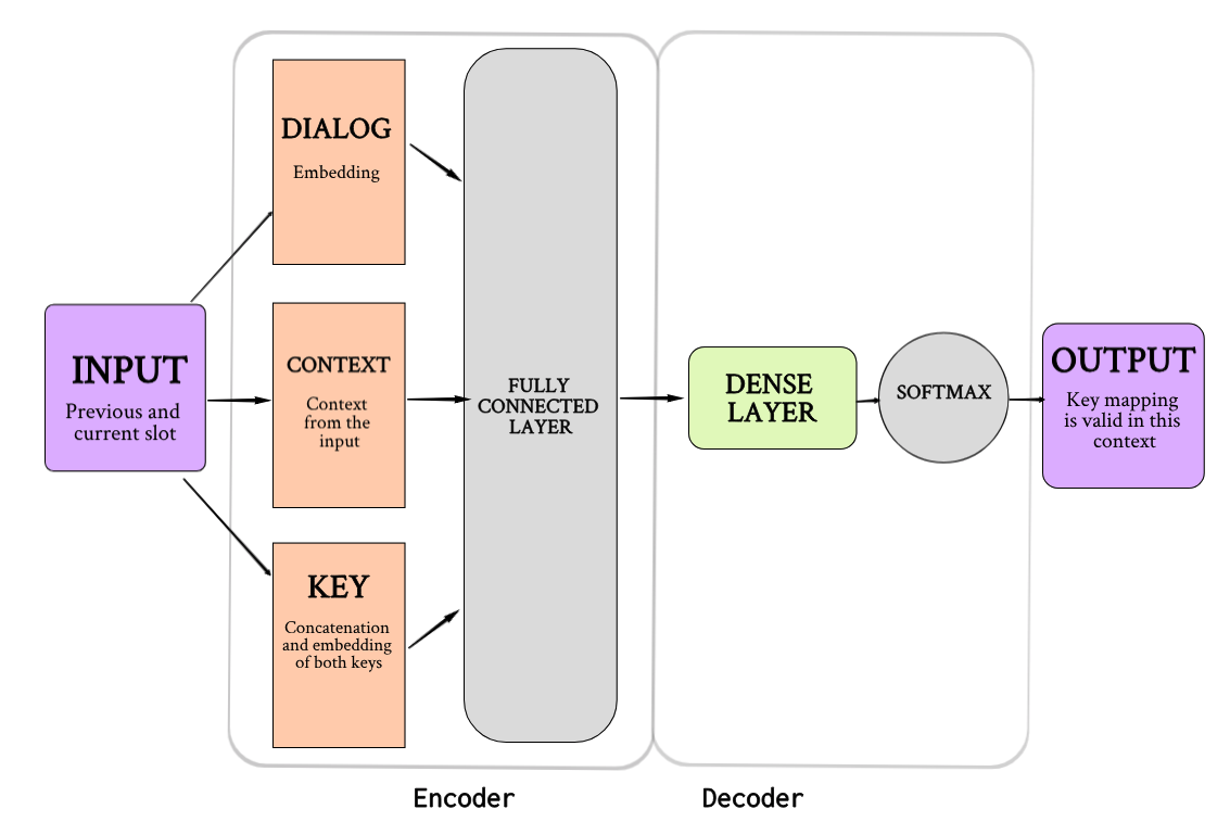
Figure 2: MLP: a model that takes in two slots, and determines whether there is a mapping between them. If so, the target slot is passed in to SC for evaluation

The three mapping strategies are trained in two OOV settings, 0% and 100%, where the OOV percentage determines the proportion of keys excluded from the training set. The resulting models are used to classify a corpus from which we generate the training datasets for SC. For our approach, in high OOV proportions we are performing zero-shot learning, so all the datasets are constrained to be $k=3$ random samples for each of the non-OOV keys. We accept or reject possible keys based on the learned threshold $\tau$.

3.2 Results

We train SC in all six datasets, and evaluate it on a fixed test set. We do not retrain the embeddings used by SC. The $F_{1}$ and accuracy scores across datasets are displayed in Table 2. The difference between HM and MLP is negligible, and we can conclude that the MLP learns the mappings properly. This means as well that MLP is bounded by the performance of HM: it is only as good as the underlying probability distribution, and will asymptotically perform the same, regardless of the OOV percentage. In contrast, our approach assigns a hypernym-based namespace to the data. In the 100% OOV case, this approach vastly outperforms both strategies. This is likely due to the fact that it is able to inject its own, semantically-related, slot key namespace into SC. This also would explain the lower performance in the 0% OOV setting.

4 Conclusions

We presented a model that employs KBs to make better decisions when facing unseen slot keys and values. This approach does not rely on a schema, as it uses the underlying slot key and value attributes, in addition to the given context. We were also able to learn a distance function for the spaces without making any assumptions other than a hierarchical relation. Leveraging KBs means that the vocabulary of this model can be expanded as-needed. This allows its vocabulary to be updated frequently, and without the need to retrain it.

Appendix A Sample Input and Output

Training input:

As an example, two input triples could be: (“Clint Eastwood”, “an American actor, filmmaker, musician, and politician”,“Actor”) and (“Clint Eastwood”, “a song by British virtual band Gorillaz”, “Song”). During inference, the target slot key is not present and the context is leveraged to disambiguate between prospective slot keys.

Constructing the tensors:

Following the example from above, our input slot value will be $w=$ “Clint Eastwood”. Assume our KB set is $\mathcal{K}=\{KB_{\text{Personalities}},KB_{\text{Songs}},KB_{\text{Companies}}\}$. Our feature tensor $\mathcal{F}$ is then composed of three sets of related terms, each corresponding to a $KB_{i}\in\mathcal{K}$, as “Clint Eastwood” is a personality commonly identified as an actor, director, and composer for various films, and was mayor of Carmel-by-the-Sea, CA. In addition, “Clint Eastwood” is also a song by the group Gorillaz that came out in the year 2001. On the other hand, no companies exist under such name, and hence the $\mathcal{F}_{\text{Companies},:,}$ entry will be empty. Note that we might have overlapping values for certain attributes: e.g., $\mathcal{F}_{\text{{personality}, \emph{actor}, birth date}}=\mathcal{F}_{\text{{personality}, \emph{mayor}, birth date}}$, which will allow us in turn to discern the features that are relevant for a given slot key.

To construct the hypernym tensor we perform a lookup of all the hypernyms for the associated terms in $\mathcal{F}$, and we include the type of KB. For example, for $\mathcal{F}_{\text{{songs}}}$, the hypernym vector will be $\mathcal{H}_{\text{{songs}}}=[\text{song, music, musical composition}]$.

Sample output:

Outputs for our model differ drastically from these of the HM and MLP methods, as it can be seen in Table 3. This is mostly due to the fact that the input (target) label $\ell$ is used as a disambiguation guide, rather than an absolute objective, and the output is a concatenation of all the hypernyms found.

Value	HM	MLP	Our approach
“rafi mecartin”	HumanBeing	HumanBeing	WriterDirectorArtist
“ryan allen”	HumanBeing	HumanBeing	ArtistBand
“raymond”	WeatherLocationCity	WeatherLocationCity	Company

Table 3: Sample labels emitted by the three different methods employed, for the same value and context. Note how, for the value “raymond”, our approach placed too much emphasis on the forklift company, rather than in the geographical location, even when the context (not pictured) clearly requested weather information.

Appendix B An Analysis of the Bregman Module

The purpose of the Bregman module is to provide a space-agnostic, learnable metric. We considered more complex approximators to the gradient, such as the Runge-Kutta methods, and variations upon gradient descent Sutskever et al. (2013). However, due to heavy calculation times we opted for the symmetric difference quotient approach described in the paper. Other approaches to approximate the Bregman divergence, such as boosting a set of the most commonly used Bregman divergences, were considered and discarded due to their lack of ability to generalize to unseen spaces.

Appendix C Ablation studies

We performed ablation studies in both the threshold $\tau$ and in the Bregman module. The inclusion of the threshold increased accuracy by 11% in our test dataset. The Bregman module was compared with two simple metrics: squared Euclidean norm and the squared difference. The inclusion of the module increased accuracy by 1% in our test dataset.

Appendix D Training Parameters

We have as trainable parameters the parameters of our Bregman module–with the exception of the step size $\epsilon$–the threshold $\tau$, and the Bi-LSTM parameters. For the initialization of the Bi-LSTMs, we used Xavier Glorot and Bengio (2010), and a recurrent dropout of $0.5$Gal and Ghahramani (2016). They have all an input size of $400$, and a hidden size of $200$. The Bregman module was initalized with random orthonormal matrices Saxe et al. (2013), and with an input size of $512$, output size of $1$, and a depth of $10$. The threshold is initialized to $\tau=0.75$, and we use Adam Kingma and Ba (2014) as our optimizer. We trained the model for $50$ epochs, with an early termination of $10$ epochs. We maintained the maximum number of hypernyms fixed at $9$, the depth of the Wordnet graph at $2$, and the features at $10$.

References

- Akata et al. (2013) Zeynep Akata, Florent Perronnin, Zaid Harchaoui, and Cordelia Schmid. 2013. Label-embedding for attribute-based classification. In Proc. IEEE CVPR 2013, CVPR ’13, pages 819–826.
- Banerjee et al. (2005) Arindam Banerjee, Srujana Merugu, Inderjit S. Dhillon, and Joydeep Ghosh. 2005. Clustering with bregman divergences. volume 6, pages 1705–1749. JMLR.org.
- Brinton (2000) Laurel J. Brinton. 2000. The Structure of Modern English: A Linguistic Introduction. John Benjamins Publishing Company.
- Fu et al. (2014) Ruiji Fu, Jiang Guo, Bing Qin, Wanxiang Che, Haifeng Wang, and Ting Liu. 2014. Learning semantic hierarchies via word embeddings. In Proc. of the 52nd Annual Meeting of the ACL, pages 1199–1209, Baltimore, Maryland. ACL.
- Gal and Ghahramani (2016) Yarin Gal and Zoubin Ghahramani. 2016. A theoretically grounded application of dropout in recurrent neural networks. In Proc. of the 30th NIPS, NIPS’16, pages 1027–1035.
- Glorot and Bengio (2010) Xavier Glorot and Yoshua Bengio. 2010. Understanding the difficulty of training deep feedforward neural networks. In Proc. of the 13th AISTATS, volume 9 of Proceedings of Machine Learning Research, pages 249–256, Sardinia, Italy.
- Graves et al. (2013) Alex Graves, Abdel-rahman Mohamed, and Geoffrey E. Hinton. 2013. Speech recognition with deep recurrent neural networks. CoRR, abs/1303.5778.
- Kingma and Ba (2014) Diederik P. Kingma and Jimmy Ba. 2014. Adam: A method for stochastic optimization. CoRR, abs/1412.6980.
- Lee et al. (2015) Joonseok Lee, Ariel Fuxman, Bo Zhao, and Yuanhua Lv. 2015. Leveraging knowledge bases for contextual entity exploration. In KDD.
- Mikolov et al. (2013) Tomas Mikolov, Ilya Sutskever, Kai Chen, Greg S Corrado, and Jeff Dean. 2013. Distributed representations of words and phrases and their compositionality. In Advances in Neural Information Processing Systems 26, pages 3111–3119.
- Miller (1995) George A. Miller. 1995. Wordnet: A lexical database for english. Commun. ACM, 38(11):39–41.
- Murty et al. (2018) Shikhar Murty, Patrick Verga, Luke Vilnis, Irena Radovanovic, and Andrew McCallum. 2018. Hierarchical losses and new resources for fine-grained entity typing and linking. In ACL.
- Naik et al. (2018) Chetan Naik, Arpit Gupta, Hancheng Ge, Mathias Lambert, and Ruhi Sarikaya. 2018. Contextual slot carryover for disparate schemas. In Proc. Interspeech 2018, pages 596–600.
- Nair and Hinton (2010) Vinod Nair and Geoffrey E. Hinton. 2010. Rectified linear units improve restricted boltzmann machines. In Proc. of the 27th ICML, ICML’10, pages 807–814.
- Nickel and Kiela (2017) Maximilian Nickel and Douwe Kiela. 2017. Poincaré embeddings for learning hierarchical representations. volume abs/1705.08039.
- Pennington et al. (2014) Jeffrey Pennington, Richard Socher, and Christopher D Manning. 2014. GloVe: Global vectors for word representation. In EMNLP, volume 14, pages 1532–1543.
- Saxe et al. (2013) Andrew M. Saxe, James L. McClelland, and Surya Ganguli. 2013. Exact solutions to the nonlinear dynamics of learning in deep linear neural networks. CoRR, abs/1312.6120.
- Shi et al. (2018) Yaxin Shi, Donna Xu, Yuangang Pan, and Ivor W. Tsang. 2018. Multi-context label embedding. CoRR, abs/1805.01199.
- Snell et al. (2017) Jake Snell, Kevin Swersky, and Richard S. Zemel. 2017. Prototypical networks for few-shot learning. CoRR, abs/1703.05175.
- Sutskever et al. (2013) Ilya Sutskever, James Martens, George Dahl, and Geoffrey Hinton. 2013. On the importance of initialization and momentum in deep learning. In Proc. of the 30th ICML, volume 28 of Proceedings of Machine Learning Research, pages 1139–1147, Atlanta, Georgia, USA. PMLR.
- Xu and Hu (2018) Puyang Xu and Qi Hu. 2018. An end-to-end approach for handling unknown slot values in dialogue state tracking. In Proceedings of the 56th Annual Meeting of the Association for Computational Linguistics (Volume 1: Long Papers), pages 1448–1457, Melbourne, Australia. Association for Computational Linguistics.
- Yang and Mitchell (2017) Bishan Yang and Tom Mitchell. 2017. Leveraging knowledge bases in lstms for improving machine reading. In Proceedings of the 55th Annual Meeting of the ACL, pages 1436–1446, Vancouver, Canada. ACL.
- Yogatama et al. (2015) Dani Yogatama, Daniel Gillick, and Nevena Lazic. 2015. Embedding methods for fine grained entity type classification. In Proc. of the 53rd Annual Meeting of the ACL and the 7th IJCNLP, pages 291–296, Beijing, China. ACL.