Singular continuous Cantor spectrum for magnetic quantum walks

Abstract

In this note, we consider a physical system given by a two-dimensional quantum walk in an external magnetic field. In this setup, we show that both the topological structure as well as its type depend sensitively on the value of the magnetic flux $\Phi$: while for $\Phi/(2\pi)$ rational the spectrum is known to consist of bands, we show that for $\Phi/(2\pi)$ irrational the spectrum is a zero-measure Cantor set and the spectral measures have no pure point part.

I Introduction

Electrons moving in a two-dimensional lattice under the influence of a uniform magnetic field are among the most intensively studied physical systems of the last decades, see e.g. brown1964bloch ; hof76 ; TKNN ; Laughlin . The Almost-Mathieu Operator (and more generally the Extended Harper’s Model) is one example of such a model which inspired intense study in mathematics; see AJ2009Ann ; AJM2017Inv ; MJ2017ETDS ; J1999Ann and references therein. Despite the simplicity of the setup its dynamical properties are surprisingly rich, and the propagation behaviour as well as the spectrum depend crucially on properties of the magnetic field like the rationality of its flux.

A similarly drastic dependence of the spectral and dynamical properties on a system parameter has recently been observed in quantum walks subject to external electric fields ewalks ; anders_loc . Quantum walks are discrete-time analogues of the unitary dynamics of a single particle with internal degree of freedom on a lattice constrained to finite propagation speed per time step aharonov1993quantum ; Ambainis2001 ; Grimmet ; TRcoin . Also, quantum walks have shown to be a useful model for quantum simulation encompassing a variety of single-particle and few-particle quantum effects such as ballistic transport, decoherence, Anderson localization and graphene-like dispersion relations as well as the formation of bound states and symmetry protected topological phases dynlocalain ; Joye2011 ; Joye_Merkli ; dynloc ; F2017CMP ; molecules ; moleculestheothers ; SpaceTimeCoinFlux ; TRcoin ; UsOnTop_short ; UsOnTop_long ; UsOnTI . At the same time quantum walks and their time-continuous counterpart are relevant in a quantum algorithmical context, for example in search algorithms, to examine the distinctness of elements, in quantum information processing and applications to the graph isomorphism problem childs2003exponential ; ambainis2003quantum ; Lovett:2010ff ; childs2009universal ; berry2011two ; portugal2018quantum . From a mathematical point of view, quantum walks on a one-dimensional lattice can also be seen as a particular class of CMV matrices giving a link between quantum dynamical systems and orthogonal polynomials on the unit circle, a connection which has proved to be fruitful in both directions BGVW ; CGMV ; CGMV2 ; GVWW ; WeAreSchur ; cedzich2015quantum . One can use spectral methods to deduce bounds on spreading DFO ; DFV . On the other hand, estimates of a dynamical nature can be turned into estimates on spectral quantities, for example, quantitative regularity of the spectral measures DEFHV .

Recently, the coupling of quantum walks to electromagnetic fields was implemented by extending the minimal coupling principle to the discrete setting UsOnELM , which allows one to analyze the reaction of a given quantum walk dynamics to an electromagnetic field. As already mentioned, for one dimensional systems the dynamics depends crucially on the rationality of the electric field: For rational fields the spectrum is absolutely continuous and the propagation is eventually ballistic after an initial segment with revivals of any initial state similar to Bloch oscillations. If the electric field is irrational the characterization is more involved and depends on the approximability of the field in terms of continued fractions: for well approximable fields the spectrum is singular continuous and the propagation is hierarchical, i.e. there is an infinite sequence of better and better revivals alternating with farther and farther excursions ewalks . On the other hand, for badly approximable fields the system displays Anderson localization which even turns out to be the typical case anders_loc .

Going beyond one spatial dimension, for the Hamiltonian setting, it is possible to connect the spectrum of the two dimensional magnetic Laplacian with the spectrum of the almost Mathieu operator, allowing to analyze not only the spectral type, but also its topological structure. Taking these questions as a starting point, we discuss in this paper in detail two-dimensional quantum walks which we place into homogeneous magnetic fields using the aforementioned discrete analogue of minimal coupling from UsOnELM . Also in the magnetic case the spectral and dynamical properties depend crucially on the rationality of the field, but this dependence turns out to be slightly less involved than for the electric walks in ewalks ; anders_loc : for rational fields the system is effectively translation invariant which by general arguments implies absolutely continuous spectrum and ballistic transport. For irrational fields, the spectrum is purely singular continuous which by the RAGE theorem cyconschroeder excludes any form of localization and thereby contrasts the typicality of Anderson localization for one-dimensional electric walks; see also FO2017JFA for a proof of the RAGE theorem in the discrete-time (unitary) case.

The paper is organized as follows: in Section II we define the system under consideration and state the main result in Theorem II.3. The proof of this theorem is divided into Section III and Section IV.

II The system

II.1 The physical model

Quantum walks describe the time-discrete evolution of a single particle with an internal degree of freedom on a lattice under the additional assumption of a finite propagation speed. In this paper, we consider particles on the two-dimensional lattice ${\mathbb{Z}}^{2}$ with two-dimensional internal degree of freedom ${\mathbb{C}}^{2}$. Basis vectors of the corresponding Hilbert space ${\mathcal{H}}=\ell^{2}({\mathbb{Z}}^{2})\otimes{\mathbb{C}}^{2}$ are denoted by $|x,s\rangle$ with $x\in{\mathbb{Z}}^{2}$ and $s=\pm 1$, and the coordinates of $\psi\in{\mathcal{H}}$ with respect to this basis are denoted by $\psi(x,\pm)\equiv\langle x,\pm 1|\psi\rangle$. A single timestep is implemented by the unitary operator

$$W_{0}=S_{1}C_{1}S_{2}C_{2},$$ (1)

where the coin operators $C_{j}=\bigoplus_{x\in{\mathbb{Z}}^{2}}C_{j}(x)$ locally rotate the internal degree of freedom as

$$C_{j}(x)=\begin{pmatrix}c^{j}_{11}(x)&c^{j}_{12}(x)\\ c^{j}_{21}(x)&c^{j}_{22}(x)\end{pmatrix}.$$

If not otherwise noted, in this paper we assume the coins to be translation invariant which means they act the same everywhere. Concretely, we take $C_{1}=C_{2}={\leavevmode\rm 1\mkern-5.4muI}\otimes C_{H}$ where $C_{H}$ is the two-dimensional Hadamard matrix

$$C_{H}=\frac{1}{\sqrt{2}}\begin{pmatrix}1&\hphantom{-}1\\ 1&-1\end{pmatrix}.$$ (2)

In contrast to the coin operators, the state-dependent shifts $S_{\alpha},\>\alpha=1,2,$ relate neighbouring cells. They are defined by $S_{\alpha}=\sum_{s=\pm 1}t_{\alpha}^{s}\otimes P_{s}$ where $t_{\alpha}|x\rangle=|x+e_{\alpha}\rangle$ denotes the lattice translation in direction $e_{\alpha}$ and $P_{\pm 1}$ projects onto the internal basis state $|\pm 1\rangle$.

The aim of this paper is to study the walk $W_{0}$ in external magnetic fields. Since $W_{0}$ is given as a sequence of coin and shift operators, such fields are introduced by an approach similar to the minimal coupling scheme in continuous time UsOnELM . This amounts to replacing the lattice translations $t_{\alpha}$ in the definition of the $S_{\alpha}$ by the unitary magnetic translations

$$T_{\alpha}|x\rangle=t_{\alpha}U_{\alpha}(x)|x\rangle=U_{\alpha}(x)|x+e_{\alpha}\rangle.$$ (3)

Here, the $U_{\alpha}(x)$ are position- and direction-dependent phases which are determined only up to a discrete gradient $G(x+e_{\alpha})G(x)^{-1}$ reflecting the freedom of local $U(1)$-gauge transformations $G:|x\rangle\mapsto G(x)|x\rangle$. In contrast to the lattice translations $t_{\alpha}$, the magnetic translations $T_{\alpha}$ do not commute anymore. Instead, they commute up to a plaquette phase, i.e.

$$T_{\alpha}^{*}T_{\beta}^{*}T_{\alpha}T_{\beta}|x\rangle=U_{\alpha}(x)^{*}U_{\beta}(x+e_{\alpha})^{*}U_{\alpha}(x+e_{\beta})U_{\beta}(x)|x\rangle=e^{-iF_{\alpha\beta}(x)}|x\rangle.$$ (4)

This commutator is invariant under local gauge transformations and we naturally call $F_{\alpha\beta}=-F_{\beta\alpha}\in[0,2\pi[$ a discrete magnetic field UsOnELM . Throughout this manuscript, we assume this magnetic field to be homogeneous, i.e. independent of $x$, and denote it by $F_{12}=:\Phi$. Note that since there are no electric fields present, a discrete version of the homogeneous Maxwell equations implies that $\Phi$ is not only homogeneous but also static, i.e. independent of time UsOnELM . If not otherwise stated, in this manuscript we fix the gauge to the symmetric gauge

$$U_{1}(x)=e^{-ix_{2}\Phi/2},\quad U_{2}(x)=e^{ix_{1}\Phi/2}.$$ (5)

After applying this discrete minimal coupling procedure to $W_{0}$ a single timestep is implemented by the magnetic walk

$$W_{\Phi}=\begin{pmatrix}T_{1}&\\ &T_{1}^{*}\end{pmatrix}C_{H}\begin{pmatrix}T_{2}&\\ &T_{2}^{*}\end{pmatrix}C_{H}.$$ (6)

Remark II.1.

The choice of gauge in (5) ensures that the phase $U_{\alpha}(x)$ commutes with $t_{\alpha}$ in (3) which allows us to interpret the magnetic walk $W_{\Phi}$ as a walk of the form (1) with quasi-periodic coins

$$C_{j}=\bigoplus_{x\in{\mathbb{Z}}^{2}}e^{(-1)^{j}i\Phi x_{k}\sigma_{3}/2}\cdot C_{H},\qquad j,k=1,2,\ j\neq k,$$ (7)

where $\sigma_{3}$ is the third Pauli matrix. Let us note for later use that the coins in (7) are never purely (off-)diagonal.

For rational fields $\Phi/(2\pi)=p/q$ the magnetic walk $W_{\Phi}$ is translation invariant after regrouping and can thus be diagonalized in momentum space UsOnRat_fields . Its spectrum is absolutely continuous and consists of $2q$ bands which resemble a two-fold copy of the Hofstadter butterfly, see Figure 1. For $\Phi/(2\pi)$ irrational, arguments similar to those in Hofstadter’s original paper hof76 immediately lead one to conjecture Cantor spectrum for $W_{\Phi}$. It is the goal of this paper to prove this conjecture and characterize the spectral type of $W_{\Phi}$ for $\Phi/(2\pi)$ irrational.

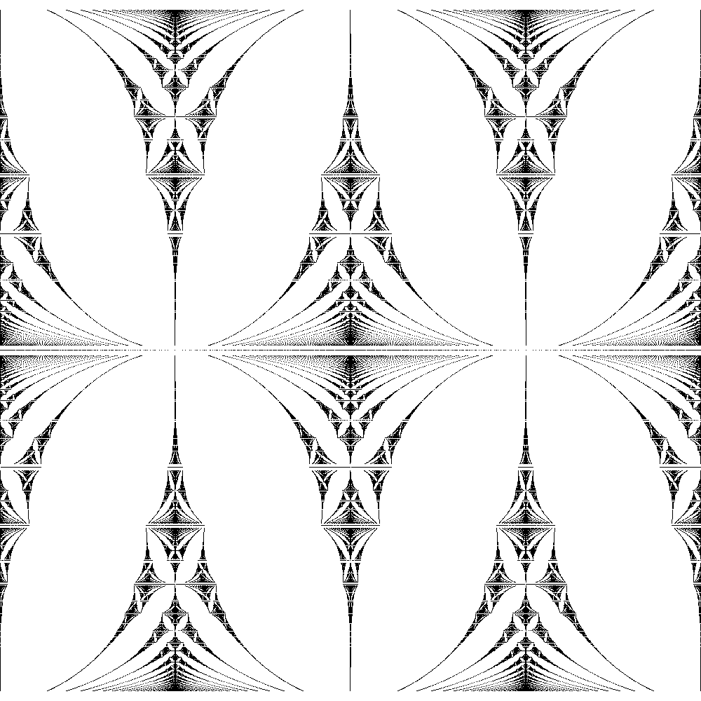
Figure 1: The spectra of the two-dimensional magnetic walk (6) for rational fields christalk resembles a two-fold copy of the Hofstadter butterfly. The vertical axis corresponds to the field $\Phi$ (plotted up to denominator 70) and the horizontal axis to the argument of the quasi-energy. Its fractal structure is evident. The symmetry of the spectrum with respect to $\Phi\mapsto-\Phi$ follows from general arguments about the rotation algebra Rieffel_Irrat_Rot , and the symmetry with respect to $z\mapsto z^{*}$ is a consequence of $KW_{\Phi}K=W_{-\Phi}$, where $K$ denotes complex conjugation, together with $\sigma(W_{\Phi})=\sigma(W_{-\Phi})$. Finally, the symmetry with respect to $z\mapsto-z$ is a consequence of $JW_{\Phi}J=-W_{\Phi}$, where $J$ is the unitary involution $J|x,s\rangle=(-1)^{x_{1}+x_{2}}|x,s\rangle$.

II.2 The rotation algebra point of view

In order to get a handle on the spectral properties of $W_{\Phi}$ we sometimes adopt an algebraic approach. The magnetic translations $T_{1}$ and $T_{2}$ realize a particular instance of the so-called rotation algebra $\mathcal{A}_{\Phi}$ which is defined abstractly as the universal $C^{*}$-algebra generated by two unitary elements $u,v$ such that

$$uv=e^{-i\Phi}vu.$$ (8)

This correspondence is established by the representation $\pi_{2}:\mathcal{A}_{\Phi}\to{\mathcal{B}}(\ell^{2}({\mathbb{Z}}^{2}))$ given by the magnetic translations

$$\pi_{2}(u)=T_{1},\quad\pi_{2}(v)=T_{2}.$$ (9)

Let us point out that the subscript on the representation refers to the dimension of the lattice in the codomain.

Denoting by $\mathbb{M}_{2}(\mathcal{A}_{\Phi})=\mathbb{M}_{2}({\mathbb{C}})\otimes\mathcal{A}_{\Phi}$ the ring of $\mathcal{A}_{\Phi}$-valued $2\times 2$-matrices, this representation of $\mathcal{A}_{\Phi}$ can be lifted to a map $\Pi_{2}:\mathbb{M}_{2}(\mathcal{A}_{\Phi})\to\mathbb{M}_{2}({\mathcal{B}}({\mathcal{H}}))$ which acts on $a=\sum_{i,j=1,2}e_{ij}\otimes a_{ij}\in\mathbb{M}_{2}(\mathcal{A}_{\Phi})$ as

$$\Pi_{2}(a)=\sum_{i,j=1,2}e_{ij}\otimes\pi_{2}(a_{ij}),$$ (10)

where $e_{ij}$ denotes the matrix whose $(i,j)$ entry is 1 and all others are $0$. Clearly, $\Pi_{2}$ is a $*$-representation because $\pi_{2}$ is. Then, we can interpret the magnetic walk $W_{\Phi}$ as the image under $\Pi_{2}$ of the unitary element $w_{\Phi}\in\mathbb{M}_{2}(\mathcal{A}_{\Phi})$ given by

$$w_{\Phi}=\begin{pmatrix}u&\\ &u^{*}\end{pmatrix}C_{H}\begin{pmatrix}v&\\ &v^{*}\end{pmatrix}C_{H}=\frac{1}{2}\begin{pmatrix}u(v+v^{*})&u(v-v^{*})\\ u^{*}(v-v^{*})&u^{*}(v+v^{*})\end{pmatrix}.$$ (11)

The abstract point of view in terms of the rotation algebra proves helpful in establishing the main result of this paper. Indeed, the first statement in Theorem II.3 below is a purely topological result which is independent of the particular representation of the rotation algebra.

Remark II.2.

The algebraic point of view on homogeneous translation systems extends to magnetic walks on higher dimensional lattices. However, it is not helpful in the presence of electric fields: following the construction in UsOnELM , electric fields imply that the spatial translations $T_{\alpha}$ in (3) commute merely up to phases with the time translation $T_{0}$ in the equation of motion. However, since $T_{0}$ relates different “time slices” of ${\mathcal{H}}$ it cannot be represented as a Hilbert space operator.

II.3 The main result

In this note we prove that the spectrum of $W_{\Phi}$ is a Cantor set for $\Phi/(2\pi)$ irrational and, moreover, show that it cannot have a pure point part. To formulate this precisely:

Theorem II.3.

Let $W_{\Phi}$ be the magnetic walk defined in (6). Then:

1. For $\Phi/(2\pi)\notin{\mathbb{Q}}$ the spectrum of $W_{\Phi}$ is a zero-measure Cantor set.

2. For any magnetic field the pure point spectrum of $W_{\Phi}$ is empty.

The zero-measure statement in the theorem refers to the arc-length measure on the circle. When we say that a subset $K$ of the circle is a Cantor set, we mean that $K$ is a closed, perfect, nowhere dense subset of the circle in the standard topology thereupon. Together, these results imply the following:

Corollary II.4.

For $\Phi/(2\pi)$ irrational, the spectrum of $W_{\Phi}$ is purely singular continuous.

This follows immediately: on the one hand, the spectrum has zero Lebesgue measure and therefore cannot have an absolutely continuous component, and on the other also the pure point component is empty by the second statement in the theorem above.

The spectral characterization of $W_{\Phi}$ in this theorem is similar to the one obtained in FOZ17 for a related model. Indeed, the proof of Cantor spectrum builds on the corresponding result in FOZ17 and was inspired by shubinDML . Yet, the proof of singular continuous spectrum does not carry over straightforwardly: the model in FOZ17 is a quasi-periodic walk on the integers and the proof of the absence of pure point spectrum makes use of transfer matrix techniques. In two spatial dimensions such transfer matrix techniques are no longer available, and we have to find different techniques to exclude eigenvalues: taking an abstract algebraic point of view is inspired by ideas from the self-adjoint setting shubinDML .

The methods we use below in the proof of Cantor spectrum are restricted to the magnetic walk with local coin given by the Hadamard matrix $C_{H}$. It is an interesting question whether the statement holds also if we allow for more general coins. While we suspect it does, a proof seems to require more heavy machinery and certainly goes beyond the scope of the current project. In contrast, the proof of the absence of point spectrum below is independent of the concrete choice of the coins: it applies to magnetic walks of the form (1) with arbitrary coins except for purely diagonal and purely off-diagonal ones.

III Proof of Cantor spectrum

In this section we prove Cantor spectrum for the two-dimensional magnetic walk $W_{\Phi}$ with $\Phi/(2\pi)$ irrational, i.e. the first statement of Theorem II.3. The idea behind the proof is to relate $W_{\Phi}$ to the so-called unitary critical almost Mathieu operator which is defined as the quantum walk $\widetilde{W}_{\Phi}$ on $\ell^{2}({\mathbb{Z}})\otimes{\mathbb{C}}^{2}$ given by

$$\widetilde{W}_{\Phi}=SC_{2}(\Phi),$$ (12)

where $S$ denotes the conditional shift $S|x,s\rangle=|x+s,s\rangle$ for $x\in{\mathbb{Z}}$, $s=\pm 1$ and $C_{2}(\Phi)$ is a position-dependent coin acting locally as

$$C_{2}(\Phi,x)=e^{i(\Phi x+\theta)\sigma_{2}}=\begin{pmatrix}\cos(\Phi x+\theta)&-\sin(\Phi x+\theta)\\ \sin(\Phi x+\theta)&\hphantom{-}\cos(\Phi x+\theta)\end{pmatrix}$$ (13)

for some fixed $\theta\in{\mathbb{T}}$. Here, the subscript in the definition of $C_{2}(\Phi)$ indicates the rotation axis in ${\mathbb{C}}^{2}$. This walk was introduced in Linden2009 ; Shikano:2010id ; Shikano:2011br as a model for an inhomogeneous quantum walk, and its spectral properties have been studied extensively in FOZ17 . In particular (FOZ17, , Thm. 1.1 c):

Theorem III.1.

Let $\Phi/(2\pi)$ be irrational. Then, the spectrum of $\widetilde{W}_{\Phi}$ is a zero measure Cantor set for all $\theta$.

Crucial for the proof of this theorem are the transfer matrix techniques for one-dimensional systems, which are not available on the two-dimensional lattice. However, we can establish a relation between the one-dimensional walk $\widetilde{W}_{\Phi}$ and the two-dimensional walk $W_{\Phi}$ by considering the representation $\pi_{1}$ of $\mathcal{A}_{\Phi}$ on $\ell^{2}({\mathbb{Z}})$ given by

$$\pi_{1}(u)|x\rangle=|x+1\rangle,\qquad\pi_{1}(v)|x\rangle=e^{i(x\Phi+\theta)}|x\rangle,$$ (14)

where as above the subscript on the representation refers to the dimension of the lattice in the codomain. Similar to the definition of $\Pi_{2}$ in (10) this representation can be lifted to a representation $\Pi_{1}$ of $\mathbb{M}_{2}(\mathcal{A}_{\Phi})$. The image of $w_{\Phi}$ in this lifted representation is given by

$$\Pi_{1}(w_{\Phi})=SC_{1}(\Phi),$$ (15)

where $C_{1}(\Phi)$ is a coin operator acting locally as $C_{1}(\Phi,x)=\exp(i\Phi x\sigma_{1})$. In particular, $C_{1}(\Phi)$ is unitarily equivalent to $C_{2}(\Phi)$ by ${\leavevmode\rm 1\mkern-5.4muI}\otimes\exp(i\sigma_{3}\pi/4)$ which commutes with the shift operator $S$. Thus, up to unitary equivalence, $W_{\Phi}$ and $\widetilde{W}_{\Phi}$ are the images of the same element $w_{\Phi}$ of $\mathbb{M}_{2}(\mathcal{A}_{\Phi})$ under different representations.

The first statement in Theorem II.3 then follows from general observations about $\mathcal{A}_{\Phi}$ and $\mathbb{M}_{2}(\mathcal{A}_{\Phi})$, or more general $\mathbb{M}_{n}(\mathcal{A}_{\Phi})$, and their images under different representations. First, for $\Phi/(2\pi)$ irrational $\mathcal{A}_{\Phi}$ is simple, i.e. its only closed, two-sided ideals are trivial Rieffel_Irrat_Rot . This implies that $\mathbb{M}_{n}(\mathcal{A}_{\Phi})$ is also simple for all $n$ grillet2007abstract . The simplicity of a $C^{*}$-algebra $\mathcal{A}$ has profound consequences: it implies that all its representations are faithful, hence isometric and therefore preserve the spectrum BratelliRobinson :

Proposition III.2.

Let $\pi,\pi^{\prime}$ be representations of a simple $C^{*}$-algebra $\mathcal{A}$. Then, for any $a\in\mathcal{A}$

$$\sigma(\pi(a))=\sigma(\pi^{\prime}(a)).$$ (16)

Thus, we conclude:

Corollary III.3.

Let $\Phi/(2\pi)$ be irrational. Then $W_{\Phi}$ and $\widetilde{W}_{\Phi}$ have the same spectrum as a subset of ${\mathbb{C}}$, i.e.

$$\sigma\bigl{(}W_{\Phi}\bigr{)}=\sigma\bigl{(}\Pi_{2}(w_{\Phi})\bigr{)}=\sigma\bigl{(}\Pi_{1}(w_{\Phi})\bigr{)}=\sigma\bigl{(}\widetilde{W}_{\Phi}\bigr{)}.$$ (17)

IV Absence of point spectrum

The present section concludes the proof of Theorem II.3 by proving the second statement. Let us note that if $\Phi/(2\pi)$ is rational, then the spectral type of $W_{\Phi}$ is purely absolutely continuous and hence point spectrum is absent. Consequently, we focus on the case $\Phi/(2\pi)\notin{\mathbb{Q}}$. We will again use some ideas from the rotation algebra perspective. Choose the symmetric gauge $(U_{1},U_{2})$ as in Section II and let $\mathscr{W}_{\Phi}=\mathscr{W}_{\Phi}(T_{1},T_{2})\equiv W^{*}(T_{1},T_{2})\subseteq{\mathcal{B}}(\ell^{2}({\mathbb{Z}}^{2}))$ denote the von Neumann algebra generated by the magnetic translations $T_{1}$ and $T_{2}$.

Let us denote the center of a von Neumann-algebra $\mathscr{A}$ by $Z(\mathscr{A})$, that is, $Z(\mathscr{A})=\{a\in\mathscr{A}:ab=ba\>\forall b\in\mathscr{A}\}$. Additionally, for $n\in{\mathbb{N}}$, we define $\mathbb{M}_{n}(\mathscr{A})=\mathbb{M}_{n}({\mathbb{C}})\otimes\mathscr{A}$ to be the matrix algebra of $n\times n$ matrices with entries in $\mathscr{A}$. We first note that the center of the matrix algebra over $\mathscr{W}_{\Phi}$ is trivial:

Lemma IV.1.

If $\Phi/(2\pi)$ is irrational, the center of $\mathbb{M}_{n}(\mathscr{W}_{\Phi})$ is trivial, that is

$$Z(\mathbb{M}_{n}(\mathscr{W}_{\Phi}))=\big{\{}{\leavevmode\rm 1\mkern-5.4muI}_{n}\otimes a:a\in Z(\mathscr{W}_{\Phi})=\{\lambda{\leavevmode\rm 1\mkern-5.4muI}:\lambda\in{\mathbb{C}}\}\big{\}},$$ (18)

where ${\leavevmode\rm 1\mkern-5.4muI}_{n}$ and ${\leavevmode\rm 1\mkern-5.4muI}$ denote the identity in $\mathbb{M}_{n}({\mathbb{C}})$ and in $\mathscr{W}_{\Phi}$, respectively.

Proof.

It is straightforward to show that the center of a matrix ring over a unital algebra $\mathscr{A}$ consists of scalar multiples of the identity matrix with scalars belonging to the center of $\mathscr{A}$. A standard reference is (grillet2007abstract, , Chapter IX, Corollary 4.4). The statement thus follows from the fact that the center of $\mathscr{W}_{\Phi}$ is trivial if $\Phi/(2\pi)$ is irrational (shubinDML, , Proposition 2.2). ∎

Naturally, the foregoing lemma is false when $\Phi$ is a rational multiple of $2\pi$. For example, if $\Phi/(2\pi)=p/q$ with $p,q\in{\mathbb{Z}}$ and $q\neq 0$, then one can verify that $T_{1}^{2q},T_{2}^{2q}\in Z(\mathscr{W}_{\Phi})$.

On $\mathbb{M}_{n}(\mathscr{W}_{\Phi})$ define the trace

$$\tau_{n}=\frac{1}{n}\mathop{\rm tr}\nolimits\otimes\tau,$$ (19)

where $\tau(a):=\langle 0|a|0\rangle$ is a trace on $\mathscr{W}_{\Phi}$ which is unique if $\Phi/(2\pi)$ is irrational shubinDML , and $\mathop{\rm tr}\nolimits$ is the matrix trace. That is, $\tau_{n}(A)=n^{-1}\sum_{j=1}^{n}\tau(a_{jj})$. One can check that $\tau_{n}$ inherits all properties of $\tau$, so $\mathbb{M}_{n}(\mathscr{W}_{\Phi})$ is a ${\rm II}_{1}$-factor, like $\mathscr{W}_{\Phi}$.

An important observation is that part of (shubinDML, , Proposition 2.1 (ii)) carries over to the matrix valued case. Concretely, given $A\in\mathbb{M}_{n}(\mathscr{W}_{\Phi})$, we may write $A=\sum_{i,j=1}^{n}e_{ij}\otimes a_{ij}$, where $a_{ij}\in\mathscr{W}_{\Phi}$. For $k,\ell\in{\mathbb{Z}}^{2}$, define the matrix $A_{k\ell}\in\mathbb{M}_{n}({\mathbb{C}})$ by

$$A_{k\ell}=\sum_{i,j=1}^{n}\langle k|a_{ij}|\ell\rangle\>e_{ij}.$$ (20)

Lemma IV.2.

Let $A\in\mathbb{M}_{n}(\mathscr{W}_{\Phi})$. Then, for all $k,\ell,m\in{\mathbb{Z}}^{2}$, we have

$$A_{k\ell}e^{-i\frac{\Phi}{2}k\wedge\ell}=A_{(k+m),(\ell+m)}e^{-i\frac{\Phi}{2}(k+m)\wedge(\ell+m)}$$ (21)

where $k\wedge\ell=k_{1}\ell_{2}-k_{2}\ell_{1}$ denotes the skew product in ${\mathbb{Z}}^{2}$. In particular, $A_{\ell\ell}=A_{mm}$ for all $\ell,m\in{\mathbb{Z}}^{2}$.

Proof.

This follows immediately from (shubinDML, , Proposition 2.1) with $\alpha=\Phi/(2\pi)$ (compare (shubinDML, , Equation (2.3)) with (8)). ∎

Remark IV.3.

The reader should notice that Lemma IV.2 is a statement about a representation of $\mathcal{A}_{\Phi}$, not about $\mathcal{A}_{\Phi}$ itself. Thus, Lemma IV.2 yields statements that (ostensibly, at least) depend on the choice of gauge. However, we will only use the diagonal case $k=\ell$, which simply says $A_{\ell\ell}=A_{mm}$ for all $m,\ell\in{\mathbb{Z}}^{2}$ and does not depend on the gauge.

We can now define the spectral distribution function (SDF) for the magnetic walk $W_{\Phi}$, which we can (and do) view as an element of $\mathbb{M}_{2}(\mathscr{W}_{\Phi})$. Define a measure $dN$ on ${\mathbb{T}}$ by

$$\int_{\mathbb{T}}g\,dN=\tau_{2}(g(W_{\Phi}))=\frac{1}{2}\sum_{s=\pm 1}\langle 0,s|g(W_{\Phi})|0,s\rangle,$$ (22)

for bounded Borel functions $g:{\mathbb{T}}\to{\mathbb{C}}$. The second equality follows from the explicit form of $\tau_{n}$ in (19). The SDF of $W_{\Phi}$ is the accumulation function of $dN$, that is, $N(\theta)=\int_{\mathbb{T}}\chi_{I(\theta)}\,dN$, where $I(\theta)$ denotes the arc $I(\theta)\equiv\{\exp(i\theta^{\prime}):0\leq\theta^{\prime}\leq\theta\}$ and $\chi_{I(\theta)}$ is the characteristic function of $I(\theta)$. In order to talk about the point at $\theta=0$ in a coherent fashion, we adopt the convention $N(\theta+2\pi)=N(\theta)+1$. Equivalently, we have

$$N(\theta)=\tau_{2}\left(E_{\theta}\right),\quad\theta\in[0,2\pi[,$$ (23)

where $E_{\theta}=\chi_{I(\theta)}(W_{\Phi})$. It follows that the spectrum of of $W_{\Phi}$ consists of all points of growth of $N(\theta)$, i.e.

$$\sigma(W_{\Phi})=\{\exp(i\theta):N(\theta-\varepsilon)-N(\theta+\varepsilon)>0\>\forall\varepsilon>0\}.$$ (24)

In particular, by weak continuity of the trace shubinDML , $\exp(i\theta)$ lies in the point spectrum of $W_{\Phi}$, if and only if $N$ is discontinuous at $\theta$. Consequently, proving continuity for the spectral distribution function proves the absence of point spectrum of $W_{\Phi}$. In particular, we show that:

Theorem IV.4.

The SDF of the magnetic walk $W_{\Phi}$ defined in (6) is continuous, i.e. $\sigma_{pp}(W_{\Phi})=\emptyset$.

To prove this theorem we will show, that the SDF is equal to the integrated density of state (IDS), which we then show to be continuous by the Delyon–Souillard argument delyon1984remark . There is an additional challenge present here when compared to the Hamiltonian case. Namely, the restriction of a self-adjoint operator to a subspace remains self-adjoint, but the restriction of a unitary operator need not even be normal. Thus, for our purposes, we need suitable unitary restrictions of $W_{\Phi}$ to finite $\Lambda\subset{\mathbb{Z}}^{2}$, which we achieve by decoupling the walk locally around the edge of $\Lambda$ using purely off-diagonal coins. Since this does not depend on the magnetic field but only on the neighbourhood structure, we will formulate this decoupling more generally for walks of the form (1).

In the following, let $\Lambda=\Lambda_{L}\subset{\mathbb{Z}}^{2}$ be a square of side length $2L+1$, centered at the origin of ${\mathbb{Z}}^{2}$, i.e.

$$\Lambda=\left\{x=(x_{1},x_{2})\in{\mathbb{Z}}^{2}\colon(|x_{1}|\leq L)\,\land\,(|x_{2}|\leq L)\right\},$$ (25)

for some $L>0$. The boundary $\partial\Lambda$ of $\Lambda$ is then given by the set

$$\partial\Lambda=\left\{x\in\Lambda\colon(|x_{1}|=L)\,\lor\,(|x_{2}|=L)\right\}.$$ (26)

For the unitary decoupling, we need a slightly different bounding set, namely the union of the upper and the right edges of $\Lambda_{L}$ and the lower and the left edges of $\Lambda_{L+1}$. To that end, put

$$\Delta\Lambda\equiv\partial\left\{x=(x_{1},x_{2})\in{\mathbb{Z}}^{2}\colon\left(-L-1\leq x_{1}\leq L\right)\,\land\,(-L-1\leq x_{2}\leq L)\right\}$$ (27)

Denote by $P_{L}:\ell^{2}({\mathbb{Z}})^{2}\otimes{\mathbb{C}}^{2}\to\ell^{2}(\Lambda_{L})\otimes{\mathbb{C}}^{2}$ the canonical projection.

Lemma IV.5.

Let $L\in{\mathbb{N}}$, let $\Lambda=\Lambda_{L}$ be as in (25) and let $W$ be a walk of the form (1). Then there is a walk $W_{d}$, such that $W_{L}=P_{L}W_{d}P_{L}^{*}$ is unitary on $P_{L}{\mathcal{H}}$ and $W-W_{d}$ differs from zero only on the set

$$\left(\Delta\Lambda\right)_{2}=\left\{x\in{\mathbb{Z}}^{2}:\operatorname{dist}(x,\Delta\Lambda)\leq 2\right\}.$$ (28)

Proof.

Define the coin operator $C_{d}$, which acts locally as

$$C_{d}(x)=\begin{cases}\sigma_{1}&x\in\Delta\Lambda\\ {\leavevmode\rm 1\mkern-5.4muI}_{2}&\text{else}\end{cases}$$ (29)

with $\sigma_{1}$ being the first Pauli matrix. Moreover replace $S_{\alpha},\alpha=1,2$ by

$$S_{\alpha}\mapsto\widetilde{S}_{\alpha}=S_{\alpha}^{\uparrow}C_{d}S_{\alpha}^{\downarrow},$$ (30)

where $S_{\alpha}^{\uparrow/\downarrow}$ shift the spin-up component in the positive and the spin-down component in the negative direction, respectively. The resulting walk

$$W_{d}=\left(S_{1}^{\uparrow}C_{d}S_{1}^{\downarrow}\right)C_{1}\left(S_{2}^{\uparrow}C_{d}S_{2}^{\downarrow}\right)C_{2}$$ (31)

is decoupled between every connection of $\Lambda$ and $\Lambda^{c}$, i.e. it fulfills the requirements in the Lemma, which is straightforward to check. ∎

Remark IV.6.

It follows from this proof that the asymmetry in the definition of $\Delta\Lambda$ is needed because of the left/right (up/down) asymmetry of $S_{\alpha}^{\uparrow}C_{d}S_{\alpha}^{\downarrow}$. Instead, one could have insisted on a symmetric $\Delta\Lambda$ and had to choose $\widetilde{S}_{\alpha}$ asymmetric.

Denoting by $|\Lambda|$ the number of points in a finite set $\Lambda$ and by $(\partial\Lambda)_{n}$ the elements of $\Lambda$ with distance less than $n\geq 1$ from the boundary, we write $\Lambda\to\infty$ whenever for some fixed $n\geq 1$

$$\frac{|(\partial\Lambda)_{n}|}{|\Lambda|}\to 0.$$ (32)

In particular, we note that $\Lambda_{L}\to\infty$ as $L\to\infty$. This together with the decoupling above allows us to define the density of states measure (DOS) for the magnetic walk $W_{\Phi}$ as the accumulation function of the vague limit of eigenvalue counting measures of the unitary truncations. That is, given $L$, define a measure $dk_{L}$ by $\int_{\mathbb{T}}g\,dk_{L}=(2|\Lambda_{L}|)^{-1}\mathop{\rm tr}\nolimits(g(W_{L}))$. Then, the DOS, denoted $dk$, is given by

$$\int_{{\mathbb{T}}}g\,dk=\lim_{L\to\infty}\int_{\mathbb{T}}g\,dk_{L}=\lim_{L\to\infty}\frac{1}{2|\Lambda_{L}|}\mathop{\rm tr}\nolimits(g(W_{L}))$$ (33)

for bounded Borel $g$, and $k(\theta)$ is given by

$$k(\theta)=\int_{\mathbb{T}}\chi_{I(\theta)}\,dk=\lim_{L\to\infty}\frac{1}{2|\Lambda_{L}|}\mathop{\rm tr}\nolimits\left(\chi_{I(\theta)}(W_{L})\right).$$ (34)

The existence of the limit in the definition of $k(\theta)$ follows from the arguments in pastur1980 . Important for our purpose is that $\theta\mapsto k(\theta)$ is continuous which follows from a proof similar to that in delyon1984remark :

Proposition IV.7.

Assume that the coins $C_{j}$ are either not completely diagonal or not completely off-diagonal. Then $\theta\mapsto k(\theta)$ is continuous.

Proof.

To prove the continuity of $\theta\mapsto k(\theta)$ it is enough to prove that

$$|\Lambda_{L}|^{-1}\mathop{\rm tr}\nolimits(\chi_{\{\exp(i\theta)\}}(W_{L}))\to 0,\quad\theta\in{\mathbb{T}},$$ (35)

as $L\to\infty$. Let $\Lambda=\Lambda_{L}$ be defined as in (25) and without loss, assume that the coins $C_{j}$ are not completely diagonal. Then, inside $\Lambda$ a solution $\psi$ of the generalized eigenvalue equation $W\psi=z\psi$ is uniquely determined by its values on the set

$$\{x\in\Lambda:x_{1}=-L\}\cup\{x\in\Lambda:x_{2}=-L,L-1,L\}.$$ (36)

This can be seen by explicitly evaluating the action of a walk of the form (1) with coins $C_{1}$ and $C_{2}$ at position $x\in{\mathbb{Z}}^{2}$:

$$(W\psi)(x,+) =c^{1}_{11}(x-e_{1})\left(c^{2}_{11}(x-e_{1}-e_{2})\psi(x-e_{1}-e_{2},+)+c^{2}_{12}(x-e_{1}-e_{2})\psi(x-e_{1}-e_{2},-)\right)$$ (37)

$$\quad+c^{1}_{12}(x-e_{1})\left(c^{2}_{21}(x-e_{1}+e_{2})\psi(x-e_{1}+e_{2},+)+c^{2}_{22}(x-e_{1}+e_{2})\psi(x-e_{1}+e_{2},-)\right)$$

$$(W\psi)(x,-) =c^{1}_{21}(x+e_{1})\left(c^{2}_{11}(x+e_{1}-e_{2})\psi(x+e_{1}-e_{2},+)+c^{2}_{12}(x+e_{1}-e_{2})\psi(x+e_{1}-e_{2},-)\right)$$ (38)

$$\quad+c^{1}_{22}(x+e_{1})\left(c^{2}_{21}(x+e_{1}+e_{2})\psi(x+e_{1}+e_{2},+)+c^{2}_{22}(x+e_{1}+e_{2})\psi(x+e_{1}+e_{2},-)\right).$$

The algorithm to determine a solution $\psi$ for $W\psi=z\psi$ inside $\Lambda$ from its values on the set (36) is as follows: first, by (37), the values of a solution $\psi$ on the set (36) immediately determine the values of $\psi(x,+)$ for $\{x:x_{1}=-L+1,x_{2}=-L+2,\dots,L-2\}$, see the left picture in Figure 2.

In the second step the values of $\psi(x,-)$ are determined subsequently for $x_{1}=-L+1$ ,$x_{2}=L-2,L-3\dots,-L+1$. The key point is this: if $\psi$ solves the generalized eigenvalue equation, then, since neither $C_{1}$ nor $C_{2}$ is completely diagonal, $\psi(x,-)$ is uniquely determined by $\psi(x,+)$, $\psi(x-e_{1}+e_{2},-)$, and $\psi(x+2e_{2},\pm)$ via (38). Concretely,

$$\begin{split}\psi(x,-)&=\frac{1}{c_{12}^{2}(x)}\bigg{[}\frac{1}{c_{21}^{1}(x+e_{2})}\Big{[}z\psi(x-e_{1}+e_{2},-)-c_{22}^{1}(x+e_{2})[c_{21}^{2}(x+2e_{2})\psi(x+2e_{2},+)\\ &\qquad\qquad\qquad+c_{22}^{2}(x+2e_{2})\psi(x+2e_{2},-)]-c_{11}^{2}(x)\psi(x,+)\Big{]}\bigg{]}.\end{split}$$ (39)

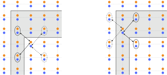
Figure 2: The algorithm to determine a generalized eigenfunction $\psi$ of $W_{0}$ of the form (1) in the proof of Proposition IV.7. At each lattice site $x\in{\mathbb{Z}}^{2}$ the internal degrees of freedom of $\psi$ are distinguished by the colouring orange for $\psi(x,+)$ and blue for $\psi(x,-)$. The arrows indicate which degrees of freedom are coupled by the action of $W$ (compare with (37) and (38)), and the shaded area indicates the boundary set (36). Note that the diagonal arrows to the left and the right of $x$ disappear for diagonal coins at $x-e_{1}$ and $x+e_{1}$, respectively, whereas the anti-diagonal arrows disappear for off-diagonal coins. Left: in the first step of the algorithm $\psi(x,+)$, $x_{1}=-L+1,|x_{2}|\leq L-2$ is obtained from the boundary values $\psi(x)$, $x_{1}=-L,|x_{2}|\leq L-1$. Right: in the second step, $\psi(x,-)$, $x_{1}=-L+1$ is determined successively for $x_{2}=L-2,L-3,\dots,-L+2$ by solving the eigenvalue equation $W\psi=z\psi$ on the boundary $x_{1}=-L,x_{2}=L-1,L-2,\dots,-L+1$.

But the value of $\psi(x,+)$ on the strip $x_{1}=-L+1$, $x_{2}=L-2,L-3,\dots,-L+1$ we just calculated, and they determine $\psi(x,-)$ with $x_{1}=-L+1$ subsequently for $x_{2}=L-2,L-3,\dots,-L+1$, see the right picture in Figure 2.

Repeating this algorithm on each strip from the left to the right determines $\psi$ completely inside $\Lambda$ from its values on the set (36). We can thus repeat the argument given in delyon1984remark , namely

$$\dim(\ker(W_{L}-e^{i\theta}))\leq 2|\eqref{eq:ids_cont_boundary}|=2(8L+1)<8(2L+1)$$ (40)

where the prefactor takes into account that we have to take one strip on the left (or right) side and two on the top/botton, and that the internal degree of freedom is two-dimensional. Then, since $|\Lambda|=\left(2L+1\right)^{2}$ we have

$$\frac{1}{|\Lambda|}\mathop{\rm tr}\nolimits(\chi_{\{\exp(i\theta)\}}(W_{L}))<\frac{8}{2L+1}\to 0$$ (41)

as $\Lambda\to\infty$. ∎

Remark IV.8.

Note that under the assumption that the coins are not completely off-diagonal the proof is completely analogous after replacing the set (36) by

$$\{x\in\Lambda:x_{1}=-L\}\cup\{x\in\Lambda:x_{2}=-L,-L+1,L\}.$$ (42)

In this case we solve for $\psi(x,-)$ as in (39) but from the bottom of $\Lambda$ instead of from the top, i.e. instead of (39) we solve (38) as

$$\begin{split}\psi(x,-)&=\frac{1}{c_{22}^{2}(x)}\bigg{[}\frac{1}{c_{22}^{1}(x-e_{2})}\Big{[}z\psi(x-e_{1}-e_{2},-)-c_{21}^{1}(x-e_{2})[c_{11}^{2}(x-2e_{2})\psi(x-2e_{2},+)\\ &\qquad\qquad\qquad+c_{12}^{2}(x-2e_{2})\psi(x-2e_{2},-)]-c_{21}^{2}(x)\psi(x,+)\Big{]}\bigg{]},\end{split}$$ (43)

and apply the algorithm “upwards” instead of “downwards”. Both requirements in Proposition IV.7 are clearly met in the magnetic walk model where the coins are given in (7).

Coming back to the magnetic walk $W=W_{\Phi}$ which in the gauge (5) indeed is of the form (1), see Remark II.1, Theorem IV.4 follows from

Proposition IV.9.

For all $\theta\in[0,2\pi[$ we have

$$k(\theta)=N(\theta).$$ (44)

For the proof of the equivalence of the IDS and the SDF we need the following variant of the celebrated Levy continuity theorem which is a special case of (applebaum, , Theorem 4.2.5) for the compact group ${\mathbb{T}}$:

Lemma IV.10.

Let $\mu_{n}$, $n\in{\mathbb{N}}$ be a sequence of probability measures on ${\mathbb{T}}$. Then $\mu_{n}\xrightarrow{w}\mu$ weakly if and only if $\widehat{\mu}_{n}\to\widehat{\mu}$ pointwise, where $\widehat{\mu}_{n}$ denotes the Fourier transform of $\mu_{n}$, which is defined by $\widehat{\mu}_{n}(t)=\int_{\mathbb{T}}e^{it\theta}\mu_{n}(d\theta)$, $t\in{\mathbb{Z}}$.

Proof of Theorem IV.4.

Given $t\in{\mathbb{Z}}$ and $L\in{\mathbb{N}}$, we have

$$\langle x,s|W_{L}^{t}|x,s\rangle=\langle x,s|W^{t}|x,s\rangle,$$ (45)

for $s=\pm 1$ and $x\in\Lambda_{L}$ with $\operatorname{dist}(x,\partial\Lambda_{L})>2|t|$. This implies that

$$\lim_{L\to\infty}\frac{1}{2|\Lambda_{L}|}\sum_{x\in\Lambda}\sum_{s}\left(\langle x,s|W_{L}^{t}|x,s\rangle-\langle x,s|W^{t}|x,s\rangle\right)=0.$$ (46)

By Lemma IV.2, we have $\langle x,s|W^{t}|x,s\rangle=\langle 0,s|W^{t}|0,s\rangle$ for all $x\in{\mathbb{Z}}^{2}$ and $s=\pm 1$, and hence

$$\lim_{L\to\infty}\frac{1}{2|\Lambda_{L}|}\mathop{\rm tr}\nolimits\left(W_{L}^{t}\right)=\tau_{2}(W^{t}).$$ (47)

The expression $(2|\Lambda_{L}|)^{-1}\mathop{\rm tr}\nolimits\left(W_{L}^{t}\right)$ on the left side of this expression is equal to the Fourier transform of the measure $dk_{L}$ whereas the right side is the Fourier transform of the measure $dN$. The statement then follows from Lemma IV.10. ∎

References

- (1) Y. Aharonov, L. Davidovich, and N. Zagury. Quantum random walks. Phys. Rev. A, 48(2):1687, 1993.
- (2) A. Ahlbrecht, A. Alberti, D. Meschede, V. B. Scholz, A. H. Werner, and R. F. Werner. Molecular binding in interacting quantum walks. New J. Phys., 14:073050, 2012. arXiv:1105.1051.
- (3) A. Ahlbrecht, C. Cedzich, R. Matjeschk, V. Scholz, A. H. Werner, and R. F. Werner. Asymptotic behavior of quantum walks with spatio-temporal coin fluctuations. Quantum Inf. Process., 11:1219–1249, 2012. arXiv:1201.4839.
- (4) A. Ahlbrecht, V. B. Scholz, and A. H. Werner. Disordered quantum walks in one lattice dimension. J. Math. Phys., 52:102201, 2011. arXiv:1101.2298.
- (5) A. Ahlbrecht, H. Vogts, A. H. Werner, and R. F. Werner. Asymptotic evolution of quantum walks with random coin. J. Math. Phys., 52:042201, 2011. arXiv:1009.2019.
- (6) A. Ambainis. Quantum walks and their algorithmic applications. Int. J. Quantum Inf., 1(04):507–518, 2003. arXiv:quant-ph/0403120.
- (7) A. Ambainis, E. Bach, A. Nayak, and A. V. Watrous. One-dimensional quantum walks. In Proc. STOC ’01, pages 37–49, New York, 2001. ACM.
- (8) D. Applebaum. Probability Measures on Compact Lie Groups. Springer International Publishing, 2014.
- (9) A. Avila and S. Jitomirskaya. The ten Martini problem. Ann. Math., pages 303–342, 2009.
- (10) A. Avila, S. Jitomirskaya, and C. Marx. Spectral theory of extended harper’s model and a question by Erdos and Szekeres. Invent. Math., 210:293–339, 2017. arXiv:1602.05111.
- (11) S. D. Berry and J. B. Wang. Two-particle quantum walks: Entanglement and graph isomorphism testing. Phys. Rev. A, 83(4):042317, 2011. arXiv:1002.3003.
- (12) J. Bourgain, F. A. Grünbaum, L. Velázquez, and J. Wilkening. Quantum recurrence of a subspace and operator-valued Schur functions. Commun. Math. Phys., 329:1031–1067, 2014. arXiv:1302.7286.
- (13) O. Bratteli and D. W. Robinson. Operator Algebras and Quantum Statistical Mechanics 1. Texts and Monographs in Physics. Springer, second edition, 1987.
- (14) E. Brown. Bloch electrons in a uniform magnetic field. Phys. Rev., 133(4A):A1038, 1964.
- (15) M.-J. Cantero, F. A. Grünbaum, L. Moral, and L. Velázquez. Matrix-valued Szegő polynomials and quantum random walks. Commun. Pure Appl. Math., 63:464–507, 2010. arXiv:0901.2244.
- (16) M.-J. Cantero, F. A. Grünbaum, L. Moral, and L. Velázquez. The CGMV method for quantum walks. Quantum Inf. Process., 11:1149–1192, 2012.
- (17) C. Cedzich. Quantum walks in electric fields, 2012. Talk given at the workshop “Quantum Walks in Grenoble”.
- (18) C. Cedzich, T. Geib, F. A. Grünbaum, C. Stahl, A. H. Werner, and R. F. Werner. The topological classification of one-dimensional symmetric quantum walks. Ann. Inst. Henri Poincaré, 19(2):325–383, 2018. arXiv:1611.04439.
- (19) C. Cedzich, T. Geib, F. A. Grünbaum, C. Stahl, L. Velázquez, A. H. Werner, and R. F. Werner. Quantum walks: Schur functions meet symmetry protected topological phases. 2019. arXiv:1903.07494.
- (20) C. Cedzich, T. Geib, C. Stahl, L. Velázquez, A. H. Werner, and R. F. Werner. Complete homotopy invariants for translation invariant symmetric quantum walks on a chain. Quantum, 2:95, 2018. arXiv:1804.04520.
- (21) C. Cedzich, T. Geib, P. Tieben, and R. F. Werner. Rational magnetic fields on the lattice: Regrouping invariance. In preparation.
- (22) C. Cedzich, T. Geib, A. H. Werner, and R. F. Werner. Quantum walks in external gauge fields. J. Math. Phys., 60(1):012107, 2019. arXiv:1808.10850.
- (23) C. Cedzich, F. A. Grünbaum, C. Stahl, A. H. Werner, and R. F. Werner. Bulk-edge correspondence of one-dimensional quantum walks. J. Phys. A: Math. Theor., 49(21):21LT01, 2016. arXiv:1502.02592.
- (24) C. Cedzich, F. A. Grünbaum, L. Velázquez, A. H. Werner, and R. F. Werner. A quantum dynamical approach to matrix Khrushchev’s formulas. Commun. Pure Appl. Math., 69(5):909–957, 2016. arXiv:1405.0985.
- (25) C. Cedzich, T. Rybár, A. H. Werner, A. Alberti, M. Genske, and R. F. Werner. Propagation of quantum walks in electric fields. Phys. Rev. Lett., 111:160601, Oct 2013. arXiv:1302.2081.
- (26) C. Cedzich and A. H. Werner. Anderson localization for electric quantum walks and skew-shift CMV matrices. 2019. arXiv:1906.11931.
- (27) A. M. Childs. Universal computation by quantum walk. Phys. Rev. Lett., 102(18):180501, 2009. arXiv:0806.1972.
- (28) A. M. Childs, R. Cleve, E. Deotto, E. Farhi, S. Gutmann, and D. A. Spielman. Exponential algorithmic speedup by a quantum walk. In Proc. STOC ’03, pages 59–68. ACM, 2003. arXiv:quant-ph/0209131.
- (29) H. Cycon, R. G. Froese, W. Kirsch, and B. Simon. Schrödinger operators, with applications to quantum mechanics and global geometry. Theoretical and Mathematical Physics. Springer, Berlin, 1987.
- (30) D. Damanik, J. Erickson, J. Fillman, G. Hinkle, and A. Vu. Quantum intermittency for sparse CMV matrices with an application to quantum walks on the half-line. J. Approx. Th., 208:59–84, 2016. arXiv:1507.02041.
- (31) D. Damanik, J. Fillman, and D. Ong. Spreading estimates for quantum walks on the integer lattice via power-law bounds on transfer matrices. J. Math. Pures. Appl., 105:293–341, 2016. arXiv:1505.07292.
- (32) D. Damanik, J. Fillman, and R. Vance. Dynamics of unitary operators. J. Fract. Geom., 1:391–425, 2014. arXiv:1308.1811.
- (33) F. Delyon and B. Souillard. Remark on the continuity of the density of states of ergodic finite difference operators. Commun. Math. Phys., 94(2):289–291, 1984.
- (34) J. Fillman. Ballistic transport for limit-periodic jacobi matrices with applications to quantum many-body problems. Commun. Math. Phys., 350:1275–1297, 2017. arXiv:1603.01173.
- (35) J. Fillman and D. Ong. Purely singular continuous spectrum for limit-periodic cmv operators with applications to quantum walks. J. Funct. Anal., 272:5107–5143, 2017. arXiv:1610.06159.
- (36) J. Fillman, D. C. Ong, and Z. Zhang. Spectral characteristics of the unitary critical almost-Mathieu operator. Commun. Math. Phys., pages 1–37, 2016. arXiv:1512.07641.
- (37) P. A. Grillet. Abstract algebra, volume 242. Springer Science & Business Media, 2007.
- (38) G. Grimmett, S. Janson, and P. F. Scudo. Weak limits for quantum random walks. Phys. Rev. E, 69:026119, 2004. arXiv:quant-ph/0309135.
- (39) F. A. Grünbaum, L. Velázquez, A. H. Werner, and R. F. Werner. Recurrence for discrete time unitary evolutions. Commun. Math. Phys., 320:543–569, 2013. arXiv:1202.3903.
- (40) D. R. Hofstadter. Energy levels and wave functions of Bloch electrons in rational and irrational magnetic fields. Phys. Rev. B, 14:2239–2249, Sep 1976.
- (41) S. Jitomirskaya. Metal-insulator transition for the almost Mathieu operator. Ann. Math., 150:1159–1175, 1999. arXiv:math/9911265.
- (42) A. Joye. Random time-dependent quantum walks. Communications in Mathematical Physics, 307(1):65, Jul 2011. arXiv:1010.4006.
- (43) A. Joye. Dynamical localization for d-dimensional random quantum walks. Quantum Inf. Process., 11:1251–1269, 2012. arXiv:1201.4759.
- (44) A. Joye and M. Merkli. Dynamical localization of quantum walks in random environments. J. Stat. Phys., 140(6):1–29, 2010. arXiv:1004.4130.
- (45) P. L. Krapivsky, J. M. Luck, and K. Mallick. Interacting quantum walkers: two-body bosonic and fermionic bound states. J. Phys. A: Math. Theor., 48(47):475301, 2015. arXiv:1507.01363.
- (46) R. B. Laughlin. Quantized Hall conductivity in two dimensions. Phys. Rev. B, 23(10):5632, 1981.
- (47) N. Linden and J. Sharam. Inhomogeneous quantum walks. Phys. Rev. A, 80(5):052327, 2009. arXiv:0906.3692.
- (48) N. B. Lovett, S. Cooper, M. Everitt, M. Trevers, and V. Kendon. Universal quantum computation using the discrete-time quantum walk. Phys. Rev. A, 81:042330, 2010. arXiv:0910.1024.
- (49) C. Marx and S. Jitomirskaya. Dynamics and spectral theory of quasi-periodic Schrödinger-type operators. Ergod. Theory Dyn. Syst., 37:2353–2393, 2017. arXiv:1503.05740.
- (50) L. A. Pastur. Spectral properties of disordered systems in the one-body approximation. Commun. Math. Phys., 75(2):179–196, 1980.
- (51) R. Portugal. Quantum Walks and Search Algorithms. Springer, 2018.
- (52) M. Rieffel. -algebras associated with irrational rotations. Pac. J. Math., 93(2):415–429, 1981.
- (53) Y. Shikano and H. Katsura. Localization and fractality in inhomogeneous quantum walks with self-duality. Phys. Rev. E, 82(3):031122, 2010. arXiv:1004.5394.
- (54) Y. Shikano and H. Katsura. Notes on inhomogeneous quantum walks. AIP Conf. Proc., 1363(1):151–154, 2011. arXiv:1104.2010.
- (55) M. Shubin. Discrete magnetic laplacian. Commun. Math. Phys., 164(2):259–275, 1994.
- (56) D. J. Thouless, M. Kohmoto, M. P. Nightingale, and M. Den Nijs. Quantized Hall conductance in a two-dimensional periodic potential. Phys. Rev. Lett., 49(6):405, 1982.