Application of Pontryagin’s Minimum Principle to Grover’s Quantum Search Problem

Abstract

Grover’s algorithm is one of the most famous algorithms which explicitly demonstrates how the quantum nature can be utilized to accelerate the searching process. In this work, Grover’s quantum search problem is mapped to a time-optimal control problem. Resorting to Pontryagin’s Minimum Principle we find that the time-optimal solution has the bang-singular-bang structure. This structure can be derived naturally, without integrating the differential equations, using the geometric control technique where Hamiltonians in the Schrödinger’s equation are represented as vector fields. In view of optimal control, Grover’s algorithm uses the bang-bang protocol to approximate the optimal protocol with a minimized number of bang-to-bang switchings to reduce the query complexity. Our work provides a concrete example how Pontryagin’s Minimum Principle is connected to quantum computation, and offers insight into how a quantum algorithm can be designed.

I Introduction

Quantum computation deliberately uses the quantum-mechanical phenomena, such as superposition and entanglement, to reduce the computation time or the number of queries to accomplish certain tasks Neilson_book ; book:Kaye_book . Well known quantum algorithms include Shor’s algorithm for factoring Shor:1997:PAP:264393.264406 and Grover’s algorithm for searching an unstructured database or an unordered list Grover:1996:FQM:237814.237866 ; PhysRevLett.79.325 . While the standard paradigm for quantum computation involves a discrete sequence of unitary logic gates Deutsch_Jozsa_92 ; Simon:1997:PQC:264393.264405 ; Shor:1997:PAP:264393.264406 ; Grover:1996:FQM:237814.237866 ; PhysRevLett.79.325 ; Bennett_97 ; PhysRevLett.103.150502 there exists another paradigm, pioneered by Farhi and Gutmann PhysRevA.57.2403 , where the quantum register evolves under some designed Hamiltonian which can vary continuously in time PhysRevA.57.2403 ; PhysRevE.58.5355 ; Farhi472 ; PhysRevA.65.042308 . The concept of “continuous-time” quantum computation explicitly allows established physics principles such as the adiabatic theorem Farhi_00 ; PhysRevLett.103.080502 ; PhysRevA.90.052317 and the Trotter-Suzuki decomposition Trotter-1959 ; Suzuki1976 to guide how quantum algorithms can be designed. The adiabatic theorem is, for example, the foundation of the quantum annealing technique PhysRevE.58.5355 ; Brooke-1999 ; Santoro-2006 ; RevModPhys.80.1061 ; Johnson_2010 and the fast, non-adiabatic evolution is found to be helpful for other problems PhysRevLett.115.230501 ; Heim215 . More recently, there are quantum algorithms based on the variational principle, notably the Variational Quantum Eigensolver (VQE) Peruzzo-2014 ; PhysRevX.6.031007 ; Kandala-2017 and the Quantum Approximate Optimization Algorithm (QAOA) Farhi_14 ; PhysRevA.92.042303 ; Lin_Lin_16 . They are more fault-tolerant than quantum algorithms of the standard paradigm and are promising for Noisy Intermediate-Scale Quantum (NISQ) technology Preskill2018quantumcomputingin .

Generally, when applying quantum algorithms to solve a classical NP (non-deterministic polynomial-time) problem, we are given a quantum “problem Hamiltonian” (oracle) whose ground state is the solution of the original classical problem RevModPhys.80.1061 ; PhysRevLett.108.130501 ; Crosson_14 ; PhysRevA.94.022309 . Designing a quantum algorithm is equivalent to find a “driving Hamiltonian” and an initial state, both easily implemented, that can steer the initial state to the target state (e.g., ground state of the problem Hamiltonian) within the shortest time. From this point of view, time-optimal control book:Luenberger ; book:Liberzon ; book:GeometricOptimalControl appears to be fundamentally connected to quantum computation as both address (i) if the target state can be reached and (ii) how to reach the target state in the shortest time. Recently, Pontryagin’s Minimum Principle (PMP) book:Pontryagin has been applied to quantum state preparation PhysRevA.97.062343 and non-adiabatic quantum computation PhysRevX.7.021027 . Due to the linearity of Schrödinger’s equation, time-optimal control generally has the bang-bang form, i.e., the control takes its extreme values. Indeed, Ref. PhysRevA.97.062343 shows that the bang-bang protocol takes the minimum time to drive a two-qubit product state to the fully entangled state; Ref. PhysRevX.7.021027 establishes the connection between the bang-bang protocol and the QAOA algorithm by solving spin-glass problems; Ref. PhysRevA.98.012301 demonstrates that pulses of bang-bang type take the minimum time to cancel the second-order noise. In this paper, we formulate Grover’s problem as a time-optimal control problem and apply PMP to solve it. By recasting the problem involving only observable dynamical variables, we are able to show that the time-optimal control is of bang-singular-bang type without explicitly solving the necessary optimality conditions derived from PMP. In the language of control theory, Grover’s algorithm can be regarded as a protocol that approximates the optimal control by the bang-bang control with a minimum number of switchings. Our analysis directly applies to the system effectively involving a single qubit PhysRevA.97.062343 ; PhysRevLett.114.100801 ; PhysRevLett.118.010501 , and may provide insight into the problems of higher dimensions PhysRevX.8.031086 ; PhysRevLett.122.020601 .

The rest of the paper is organized as follows. In Section II we formulate the problem and state the necessary conditions for a time-optimal solution derived from PMP. In Section III we show that the bang-singular-bang structure satisfies the necessary conditions and compares this solution to other protocols including the pure singular control and the pure bang-bang control which turns out to be Grover’s algorithm. Advantages of numerically applying PMP to problems of higher dimensions are discussed. In Section IV we re-formulate the problem in terms of geometric control, and show that the time-optimal bang-singular-bang control can be naturally derived in this formalism. The relation to quantum state preparation are pointed out. Section V is the conclusion. In the Appendix, a few detailed steps regarding the geometric control technique are provided.

II Problem statement and Pontryagin’s Minimum Principle

In this section we formulate Grover’s problem in terms of two Hamiltonians and summarize the relevant results from PMP. Because both quantum mechanics and PMP use the term “Hamiltonian”, we shall use “Hamiltonian” (symbol $H$) in the quantum-mechanical sense, i.e., it is a matrix that governs the dynamics of the wave function; use “c-Hamiltonian” (symbol $\mathcal{H}$) to represent the control-Hamiltonian, a scalar function defined in control theory.

II.1 Problem statement

Following Ref. PhysRevA.57.2403 ; PhysRevA.65.042308 , Grover’s problem can be formulated using Hamiltonians. Given the “problem Hamiltonian” $H_{w}=|w\rangle\langle w|$ and the “driving Hamiltonian” $H_{s}=|s\rangle\langle s|$ where $\langle s|w\rangle\equiv x<1$ ($x$ and $|s\rangle$ are assumed to be real for now, and $|s\rangle$ for Grover’s problem is given in Eq. (4)), we want to find the time-optimal protocol $u(t)$ that brings the initial state $|\psi_{i}\rangle=|s\rangle$ to the target state $|\psi_{target}\rangle=|w\rangle$ for the system evolved under a time-dependent Hamiltonian

$$H(t;u) =\frac{1}{2}(H_{w}+H_{s})+u(t)\,\frac{1}{2}(H_{w}-H_{s})$$ (1)

$$\equiv H_{0}+u(t)H_{d},\text{ with }|u(t)|\leq 1.$$

The control $u(t)$ of the problem is assumed to be bounded by $|u|\leq 1$ convention . In this paper, the terms “control”, “protocol”, and “algorithm” are used interchangeably; a given control/protocol/algorithm corresponds to a specific $u(t)$. Because all non-target states are degenerate in energy, we can express both Hamiltonians using two orthogonal states $|w\rangle$, $|\bar{w}\rangle=\left[|s\rangle-x|w\rangle\right]/\sqrt{1-x^{2}}$. The initial state is given by $|\psi_{i}\rangle=|s\rangle=x|w\rangle+\sqrt{1-x^{2}}|\bar{w}\rangle$. In terms of Pauli matrices defined as

$$\sigma_{x}=\begin{bmatrix}0&1\\ 1&0\end{bmatrix},\,\,\sigma_{y}=\begin{bmatrix}0&-i\\ i&0\end{bmatrix},\,\,\sigma_{z}=\begin{bmatrix}1&0\\ 0&-1\end{bmatrix},$$

the Hamiltonians in Eq. (1) are

$$H_{w} =\frac{1}{2}(e+\sigma_{z}),$$ (2a)

$$H_{s} =\frac{1}{2}e+\frac{1}{2}\left[(2x\sqrt{1-x^{2}})\sigma_{x}+(2x^{2}-1)\sigma_{z}\right]$$ (2b)

$$H_{0} =\frac{1}{2}e+\frac{x}{2}\left[\sqrt{1-x^{2}}\sigma_{x}+x\sigma_{z}\right],$$ (2c)

$$H_{d} =-\frac{x}{2}\sqrt{1-x^{2}}\sigma_{x}+\frac{1}{2}(1-x^{2})\sigma_{z},$$ (2d)

$$|\psi_{i}\rangle =\begin{bmatrix}x\\ \sqrt{1-x^{2}}\end{bmatrix},\,\,\,|\psi_{target}\rangle=\begin{bmatrix}1\\ 0\end{bmatrix}.$$ (2e)

Note that the target state is allowed to have an arbitrary phase. For later discussions, we further define

$$H_{X} =H_{0}-H_{d}=H_{s},$$ (3)

$$H_{Y} =H_{0}+H_{d}=H_{w},$$

i.e., $H_{X}$ corresponds to $u=-1$ whereas $H_{Y}$ to $u=+1$. The initial state is chosen to be

$$|s\rangle=\frac{1}{\sqrt{N}}\sum_{k=1}^{N}|k\rangle,$$ (4)

with $N$ the dimension of search space (Hilbert space) spanned by $\{|k\rangle\}$. As Hamiltonians given in Eqs. (2) are just $2\times 2$ matrices, the problem dimension $N$ is encoded in the overlap $x=1/\sqrt{N}$. Throughout this paper, $x$ (different from $\boldsymbol{x}$) exclusively represents the overlap between the initial and the target state $\langle s|w\rangle$. The two-dimensional wave function will be referred to as a “qubit” state.

II.2 Time-optimal control problem and Pontryagin’s Minimum Principle

The necessary conditions for a time-optimal solution derived from PMP are discussed in this subsection. We focus on the control-affine control system, where the dynamics of its “state variables” $\boldsymbol{x}$ are described by

$$\dot{\boldsymbol{x}}=\mathbf{f}(\boldsymbol{x})+u(t)\,\mathbf{g}(\boldsymbol{x}),\,\,\boldsymbol{x}\in R^{n},u\in R$$ (5)

To differentiate from “quantum state”, $\boldsymbol{x}$ will be referred to as “dynamical variables”; $\mathbf{f}$ and $\mathbf{g}$ are smooth vector fields which are functions of $\boldsymbol{x}$. Control-affine system is directly related to the Schrödinger’s equation. In the language of differential geometry, $\boldsymbol{x}$ defines a manifold; $\mathbf{f}$ and $\mathbf{g}$ belong to the tangent space of that manifold. We assume the admissible range of $u$ is bounded by $|u|\leq 1$. Time-optimal control problem is defined as follows: given Eq. (5), find the optimal control $u(t)$ to minimize the cost function

$$J=\lambda_{0}\int_{0}^{t_{f}}\text{d}t+\mathcal{C}(\boldsymbol{x}(t_{f})),$$ (6)

where $t_{f}$ is the final time, $\lambda_{0}$ is a positive constant, and $\mathcal{C}(\boldsymbol{x}(t_{f}))$ is a terminal cost function depending only on the values of the dynamical variables at $t_{f}$. To make sense of a “time-optimal” solution, $\lambda_{0}$ has to be positive. We only consider the time-invariant problem where $\mathbf{f}$, $\mathbf{g}$, and $\mathcal{C}$ do not depend explicitly on time $t$.

Following PMP book:Luenberger , a control-Hamiltonian is defined as

$$\bar{\mathcal{H}}_{c}(t) =\lambda_{0}+\langle\boldsymbol{\lambda}(t),\mathbf{f}(\boldsymbol{x})\rangle+u(t)\langle\boldsymbol{\lambda}(t),\mathbf{g}(\boldsymbol{x})\rangle$$ (7)

$$\equiv\lambda_{0}+\langle\boldsymbol{\lambda}(t),\mathbf{f}(\boldsymbol{x})\rangle+u(t)\Phi(t)$$

$$\equiv\lambda_{0}+\mathcal{H}_{c}(t).$$

$\boldsymbol{\lambda}$ is referred to as a set of “costate” variables (or the conjugate momentum), which has the same dimension of $\boldsymbol{x}$. $\langle\cdot,\cdot\rangle$ is the inner product introduced for two real-valued vectors. A switching function $\Phi(t)$ is defined as

$$\Phi(t)=\langle\boldsymbol{\lambda}(t),\mathbf{g}(\boldsymbol{x})\rangle,$$ (8)

which plays the most important role in determining the structure of optimal control.

Given an optimal solution $(\boldsymbol{x}^{*},\boldsymbol{\lambda}^{*};u^{*})$ to the time-optimal control problem, it has to satisfy the following necessary conditions:

$$\dot{\boldsymbol{x}}^{*}(t)=+\left(\nabla_{\boldsymbol{\lambda}}\mathcal{H}_{c}\right),\,\,\,\boldsymbol{x}^{*}(0)\text{ is given.}$$ (9a)

$$\dot{\boldsymbol{\lambda}}^{*}(t)=-\left(\nabla_{\boldsymbol{x}}\mathcal{H}_{c}\right)^{T},\,\,\,\boldsymbol{\lambda}^{*}(t_{f})=\nabla_{\boldsymbol{x}}\mathcal{C}|_{\boldsymbol{x}^{*}(t_{f})}$$ (9b)

$$\bar{\mathcal{H}}_{c}=\lambda_{0}+\mathcal{H}_{c}=\text{ const. }$$ (9c)

$$u^{*}(t)=\begin{cases}+1&\text{ if }\Phi(t)<0\\ -1&\text{ if }\Phi(t)>0\\ \text{undetermined}&\text{ if }\Phi(t)=0\end{cases}.$$ (9d)

Let us elaborate on these necessary conditions. Eq. (9a) is identical to the dynamics defined in Eq. (5). Eq. (9b) defines the dynamics of costate variables, whose boundary condition is fixed at the final time $t_{f}$. Eq. (9c) holds for the time-invariant problem. If the final time $t_{f}$ is not fixed (i.e., $t_{f}$ is allowed to vary to minimize $\mathcal{C}$), then $\bar{\mathcal{H}}_{c}=0$. Because $\lambda_{0}$ is a positive constant, we conclude that $\mathcal{H}_{c}(t)$ has to be a negative constant for a time-optimal solution. In the following analysis, we shall focus on $\mathcal{H}_{c}$ (instead of $\bar{\mathcal{H}}_{c}$), and the condition (9c) is replaced by

$$\mathcal{H}_{c}=\text{const.}\leq 0.$$ (10)

Eq. (9d) means that the optimal control takes the extreme values ($\pm 1$ in this case) when the switching function is nonzero. This structure is referred to as “bang-bang” protocol. If $\Phi(t)=0$ over a finite interval of time, then $u$ is undetermined from Eq. (9d) and more analysis is needed. When $\Phi=0$, the time-optimal control $u^{*}$ may not take its extreme values and is referred to as a singular control. The behavior of $\Phi=0$ will be analyzed in Section IV.2 to establish the structure of time-optimal solution.

II.3 Application to the Schrödinger’s equation

In Grover’s problem, the dynamics of the wave function obey the Schrödinger’s equation

$$i\frac{\text{d}}{\text{d}t}|\Psi(t)\rangle =\left[H_{0}+u(t)\,H_{d}\right]|\Psi(t)\rangle,$$ (11)

$$\text{with }|\Psi(t)\rangle =\begin{bmatrix}\Psi_{0}\\ \Psi_{1}\end{bmatrix}=\begin{bmatrix}\Psi_{0,R}+i\Psi_{0,I}\\ \Psi_{1,R}+i\Psi_{1,I}\end{bmatrix}.$$

The initial and final states are given in Eq. (2e). To make the final state as close to $[1,0]^{T}$ as possible, the terminal cost function can be chosen as

$$\mathcal{C}(\Psi(t_{f}))=-\frac{1}{2}|\Psi_{0}(t_{f})|^{2}.$$ (12)

As explicitly shown in Eq. (11), $|\Psi\rangle$ contains four real variables. As a result costate variables $\Pi_{0,R}$, $\Pi_{0,I}$, $\Pi_{1,R}$, $\Pi_{1,I}$ are needed. It is convenient to express the four costate variables as a two-dimensional complex vector

$$|\Pi(t)\rangle=\begin{bmatrix}\Pi_{0,R}+i\Pi_{0,I}\\ \Pi_{1,R}+i\Pi_{1,I}\end{bmatrix}.$$ (13)

Using the property that $H_{0}$ and $H_{d}$ are real-valued, we can express the c-Hamiltonian and switching function as

$$\mathcal{H}_{Q,c} =\text{Im}\langle\Pi(t)|\left[H_{0}+u(t)\,H_{d}\right]|\Psi(t)\rangle,$$ (14)

$$\Phi_{Q}(t) =\text{Im}\langle\Pi(t)|H_{d}|\Psi(t)\rangle.$$

Applying Eq. (9b), one can derive that the dynamics of $|\Pi(t)\rangle$ are governed by the same Schrödinger’s equation, with the boundary condition given at $t_{f}$ PhysRevA.97.062343 ; PhysRevX.7.021027 :

$$i\frac{\text{d}}{\text{d}t}|\Pi(t)\rangle=\left[H_{0}+u(t)\,H_{d}\right]|\Pi(t)\rangle,$$ (15)

$$\text{ with }|\Pi(t_{f})\rangle=-\begin{bmatrix}\Psi_{0}(t_{f})\\ 0\end{bmatrix}.$$

The condition  (9d) still holds, with the switching function computed using Eq. (14). The subscript ‘Q’ in Eqs. (14) indicates ‘quantum’ and will be dropped from now on.

Eqs. (11) and  (12) allow us to do the bruteforce optimization to determine the optimal $u(t)$. Eqs. (14) and  (15) allow us to check if a control $u(t)$ satisfies the necessary conditions. One may expect that the optimal control is mostly of bang-bang type, as $\Phi(t)=0$ can only occupy a negligible region in the manifold. In Section III we numerically show that the optimal protocol actually has the bang-singular-bang structure.

III Optimal protocol

In this section we show that the time-optimal control has the bang-singular-bang structure. In particular, we numerically check that a solution bearing this structure satisfies all necessary conditions imposed by PMP, and explicitly show that the time-optimal solution does take a shorter time to reach the target state when compared to other known protocols.

III.1 Two existing protocols

We begin the discussion by introducing two existing protocols which will be compared to the optimal protocol described shortly. The first one is provided by Farhi and Gutmann  PhysRevA.57.2403 . By choosing $u(t)=0$ in Eq. (1), the wave function is

$$|\Psi(t)\rangle =e^{-i\frac{1}{2}(H_{s}+H_{w})t}|s\rangle$$ (16)

$$=e^{-i\frac{t}{2}}\begin{bmatrix}x\cos\frac{xt}{2}-i\sin\frac{xt}{2}\\ \sqrt{1-x^{2}}\cos\frac{xt}{2}\end{bmatrix}\equiv\begin{bmatrix}\Psi_{0}(t)\\ \Psi_{1}(t)\end{bmatrix}.$$

As $|\Psi_{0}(t)|^{2}=x^{2}\cos^{2}\frac{xt}{2}+\sin^{2}\frac{xt}{2}$, we find that for total computation time $t_{f}=\frac{\pi}{x}$, $|\Psi_{0}(t_{f})|^{2}=1$. This protocol will be referred as the “singular” control as $u$ does not take either of its extreme values. The second protocol is the celebrated Grover’s algorithm PhysRevLett.79.325 , where the initial state $|s\rangle$ is evolved by alternating $U_{w}=2|w\rangle\langle w|-I$ and $U_{s}=I-2|s\rangle\langle s|$ about $N=\frac{\pi}{4x}$ times, i.e.,

$$|\psi_{f}\rangle=(U_{s}U_{w})^{N}|s\rangle.$$ (17)

In terms of Eq. (1), $U_{w}$ is achieved by $e^{-i\pi H_{w}}$ and $U_{s}$ by $e^{-i\pi H_{s}}$ up to an irrelevant sign. The total computation time for Grover’s algorithm is therefore $(\pi+\pi)N\sim\frac{\pi^{2}}{2x}$. Grover’s algorithm and the singular protocol have the same asymptotic $x^{-1}$ behavior, but the latter has a smaller prefactor. The annealing algorithm proposed by Roland and Cerf PhysRevA.65.042308 is slower but more robust, as it applies the adiabatic theorem concerning the (instant) gap between the ground and the first excited state, but does not explicitly use the structure that all non-target states are degenerate. The annealing algorithm will not be discussed here. However, we note that the optimal $u(t)$ obtained using PMP is non-adiabatic, and the procedure does not know if there is a gap at any instant of time, which is essential for the adiabatic quantum computing.

III.2 Optimal control and analytical analysis

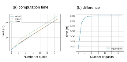
Figure 1: (Color Online) (a) The total computation time for the optimal control, the singular control, and Grover’s algorithm in logarithmic scale. For $n$ number of qubits, the overlap $x=2^{-n/2}$. For the smaller system, the optimal control has a noticeable speedup. When the system becomes large, these two methods are almost equivalent. Grover’s algorithm has the same asymptotic behavior with a larger prefactor. (b) the difference of computation time between the optimal and the singular control in linear scale. The optimal control takes less time; the difference approaches 0.436 $\pi$ at large $n$.

We claim that the time-optimal control has the bang-singular-bang structure which will be proved using geometric control in Section IV. In particular, the order is $u=+1$ (bang), $u=0$ (singular), and $u=-1$ (bang). The time periods for the initial and the final bang control are identical because the problem is unchanged if we swap the initial and target states. Let us first investigate the consequences of applying this protocol.

Assume that the time intervals of two bang controls are both $t_{1}$, and that of the singular control is $t_{2}$. The wave function at $t_{f}=2t_{1}+t_{2}$ is given by

$$|\Psi(t_{1};t_{2})\rangle =e^{-it_{1}H_{s}}e^{-i\frac{t_{2}}{2}(H_{s}+H_{w})}e^{-it_{1}H_{w}}|s\rangle\equiv\begin{bmatrix}\Psi_{0}(t_{1},t_{2})\\ \Psi_{1}(t_{1},t_{2})\end{bmatrix}$$ (18)

A straightforward calculation gives (neglecting the phase factor)

$$\Psi_{1}(t_{1},t_{2}) =\sqrt{1-x^{2}}\left[\cos\frac{xt_{2}}{2}(1-4x^{2}\sin^{2}\frac{t_{1}}{2})-2x\sin\frac{xt_{2}}{2}\sin t_{1}\right].$$ (19)

Note that maximizing $|\Psi_{0}(t_{1},t_{2})|^{2}$ is equivalent to minimizing $|\Psi_{1}(t_{1},t_{2})|^{2}$. If the target state can be exactly reached, $\Psi_{1}(t_{1},t_{2})=0$ which allows us to represent $t_{2}$ as a function of $t_{1}$:

$$\tan\frac{xt_{2}}{2}=\frac{1-4x^{2}\sin^{2}\frac{t_{1}}{2}}{2x\sin t_{1}}=\frac{1-2x^{2}+2x^{2}\cos t_{1}}{2x\sin t_{1}}.$$ (20)

As a result the total computation time can be written as a function of $t_{1}$:

$$t_{f}(t_{1})=2t_{1}+t_{2}(t_{1}).$$ (21)

A time-optimal solution requires $\frac{\text{d}t_{f}}{\text{d}t_{1}}=2+\frac{\text{d}t_{2}}{\text{d}t_{1}}=0$, from which we get $\frac{\text{d}t_{2}}{\text{d}t_{1}}=-2$. To get the optimal $t_{1}$, we take $\frac{\text{d}}{\text{d}t_{1}}$ on both sides of Eq. (20):

$$\sec^{2}(\frac{xt_{2}}{2})\cdot\frac{x}{2}\cdot\frac{\text{d}t_{2}}{\text{d}t_{1}}=\frac{1}{\cos^{2}(\frac{xt_{2}}{2})}\cdot\frac{x}{2}\cdot\frac{\text{d}t_{2}}{\text{d}t_{1}}$$ (22)

$$\Rightarrow \left[4x^{2}(x^{2}-1)\right]\cos^{2}(t_{1})+\left[-2(2x^{2}-1)^{2}\right]\cos(t_{1})+(2x^{2}-1)^{2}=0$$

Eq. (22) gives the optimal $t_{1}$. Solving Eq. (22) gives $\cos(t_{1})=\frac{-1+2x^{2}}{2x^{2}}$ or $\frac{-1+2x^{2}}{2(-1+x^{2})}$. We take the positive solution which corresponds to a smaller $t_{1}$. The time-optimal solution $(t^{*}_{1},t^{*}_{2})$ is therefore

$$\cos(t^{*}_{1})=\frac{-1+2x^{2}}{2(-1+x^{2})},\,\,\,\tan(\frac{x\,t^{*}_{2}}{2})=\frac{1-4x^{2}\sin^{2}\frac{t^{*}_{1}}{2}}{2x\sin t^{*}_{1}}.$$ (23)

Taking $x=\frac{1}{2}$, we have $\cos(t^{*}_{1})=\frac{1}{3}$ and thus $t^{*}_{1}\approx 0.392\pi$; $t^{*}_{2}\approx 0.784\pi$; $t^{*}_{f}=2t^{*}_{1}+t^{*}_{2}\approx 1.5673\pi$. For $x=\frac{1}{\sqrt{32}}$, $t^{*}_{1}\approx 0.339\pi$ and $t^{*}_{f}\approx 5.221\pi$. These values are consistent with our numerical simulations.

When $x$ is small, we get $\cos t^{*}_{1}\approx\frac{1}{2}-\frac{x^{2}}{2}$ from which we identify $t^{*}_{1}=\frac{\pi}{3}+\delta$. Matching the lowest non-vanishing order in $x$, we have

$$\cos(t^{*}_{1}) =\cos(\frac{\pi}{3}+\delta)\approx\frac{1}{2}-\delta\cdot\sin\frac{\pi}{3}=\frac{1}{2}-\frac{x^{2}}{2}$$ (24)

$$\Rightarrow \delta=\frac{1}{\sqrt{3}},\,\,\,t^{*}_{1}=\frac{\pi}{3}+\frac{x^{2}}{\sqrt{3}}.$$

To get the small-$x$ expansion of $t^{*}_{2}$, we use $\sin\theta=\frac{2\tan(\theta/2)}{1+\tan^{2}(\theta/2)}$ to write the second equation in Eq. (23) as

$$\sin(xt^{*}_{2})=2\frac{(1-4x^{2}\sin^{2}\frac{t^{*}_{1}}{2})\cdot(2x\sin t^{*}_{1})}{(1-4x^{2}\sin^{2}\frac{t^{*}_{1}}{2})^{2}+(2x\sin t^{*}_{1})^{2}}\approx 4x\sin t^{*}_{1}=2x\sqrt{3}.$$ (25)

We expand $xt^{*}_{2}\approx\pi+\delta$ to get

$$\sin(xt^{*}_{2}) =\sin(\pi+\delta)\approx-\delta=2x\sqrt{3}\Rightarrow\delta=-2x\sqrt{3}$$ (26)

$$\Rightarrow t^{*}_{2}=\frac{\pi+\delta}{x}=\frac{\pi}{x}-2\sqrt{3}.$$

The total time in the small $x$ limit is

$$2t^{*}_{1}+t^{*}_{2}=\frac{\pi}{x}+\frac{2\pi}{3}-2\sqrt{3}\approx\frac{\pi}{x}-0.436\pi.$$ (27)

Note $\pi/x$ is the total time needed in the singular protocol PhysRevA.57.2403 . Fig. 1(a) shows the total computation time for optimal bang-singular-bang control [by evaluating Eqs. (23)], the singular control and Grover’s algorithm. For $n$ number of qubits, the overlap $x=2^{-n/2}$. Their asymptotic behaviors are the same; the acceleration is only noticeable when the system is small. The time difference between the singular and the optimal control, given in Fig. 1 (b), is indeed consistent with Eq. (27).

III.3 Example of $x=1/2$

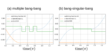
Figure 2: (Color Online) The multiple bang-bang control (a) and the optimal control (b) for $x=\frac{1}{2}$ with the total computation time $t_{f}=1.3\pi$, which is not long enough to reach the target state. In (a), the c-Hamiltonian (dashed curve) is not a constant over the time interval, and the switching function (dotted curve) and the control (solid curve) have the same sign, violating the necessary conditions derived from PMP. For the optimal bang-singular-bang control, all necessary conditions are satisfied.

More details for the $x=1/2$ case are provided. In particular, we are interested in the behavior for a fixed total time $t_{f}$ where the total cost function defined in Eq. (6) only has the terminal cost function. The case we will consider is $t_{f}=1.3\pi<t^{*}_{f}(x=1/2)\sim 1.57\pi$, i.e., it is a representative example where the computation time is too short to reach the target state. The optimal bang-singular-bang protocol is

$$u_{opt}(t;t_{1})=\begin{cases}1&\text{ for $0<t<t_{1}$}\\ 0.&\text{ for $t_{1}<t<t_{f}-t_{1}$}\\ -1&\text{ for $t_{f}-t_{1}<t<t_{f}$}\end{cases}.$$ (28)

For a given $t_{f}$, control (28) only has one parameter $t_{1}$ which will be determined by numerically minimizing the cost function. We also consider the multiple bang-bang protocol

$$u_{m}(t;t_{1},N)=\begin{cases}1&\text{ for $0<t<t_{1}$}\\ -1/1&\text{ alternate $N$ times for $t_{1}<t<t_{f}-t_{1}$}\\ -1&\text{ for $t_{f}-t_{1}<t<t_{f}$}\end{cases}.$$ (29)

Between $t_{1}<t<t_{f}-t_{1}$, the control $u$ is alternating between -1 and 1 exactly $N$ times, and each lasts $(t_{f}-2t_{1})/(2N)$. For a given $t_{f}$ and $N$, $t_{1}$ of control (29) will also be determined by numerically minimizing the cost function.

Fig. 2(a) shows the switching function $\Phi$ and the c-Hamiltonian $\mathcal{H}_{c}$ [defined in Eq. (14)] using the multiple bang-bang control (29) with $N=2$ (totally 5 switchings). The numerical optimization gives $t_{1}=0.4446\pi$. We see that for $t$ between about $0.3\pi$ and $0.9\pi$, the control $u(t)$ and the switching function $\Phi(t)$ have the same sign which violates the necessary condition (9d). Also, the c-Hamiltonian $\mathcal{H}_{c}$ is not a constant over $[0,t_{f}]$ which violates the necessary condition (10). Fig. 2(b) shows the switching function and the c-Hamiltonian using the optimal bang-singular-bang control (28). The numerical optimization gives $t_{1}=0.3918\pi$. We see that all necessary conditions are satisfied, i.e., the control $u(t)$ and the switching function $\Phi(t)$ either have opposite signs or are both zero and the c-Hamiltonian $\mathcal{H}_{c}$ is a constant over the entire $[0,t_{f}]$.

III.4 Summary and discussion on problems of higher dimensions

In this section, we have combined the analytical analysis and numerical optimization to show that the control of bang-singular-bang type satisfy all necessary conditions for a time-optimal solution. The numerical optimization involves repeating the following three steps: (i) assuming a control $u(t)$; (ii) evolving the wave function from $|\Psi(t=0)\rangle=|s\rangle$ to $|\Psi(t=t_{f})\rangle$ (by integrating a differential equation, a two-dimensional Schrödinger equation here); (iii) evaluating the cost function. To check the necessary conditions, we need to (iv) compute the conjugate momentum $|\Pi(t)\rangle$ backwards in time from $t_{f}$. If $u(t)$ contains many parameters, satisfying the necessary conditions during the entire computation time is practically impossible. Knowing the structure of the control is of great numerical value – it not only significantly decreases the optimization time by reducing the dimension of search domain but also finds a better solution (i.e., smaller cost function). In Section IV we show that the structure of optimal control can be determined even without integration for this problem.

For problems of higher dimensions, the structure of optimal control by itself can easily become prohibitively difficult to determine. Although the analytical analysis may not be possible, PMP can still be a valuable numerical tool. Specifically, by solving the Schrödinger equation two times for a given $u(t)$ – one for the wave function $|\Psi(t)\rangle$ [step (ii)] and one for the conjugate momentum $|\Pi(t)\rangle$ [step (iv)], we are able to compute the switching function that reflects the gradient of the cost function with respect to the given $u(t)$. This is known as the “adjoint state method” book:Luenberger . The gradient obtained using adjoint state method is exact (up to a numerical error), time efficient, and can be used in an iterative optimization algorithm to update $u(t)$.

IV Geometric control

The Schrödinger equation in Eq. (11) involves four (dependent) real variables, and directly applying PMP to a dynamical system of four variables is not immediately informative. In this section, we reduce the number of variables to two, and apply geometric control to derive the structure of the time-optimal solution. Grover’s algorithm will also be analyzed within this framework.

IV.1 Dimension reduction and Bloch sphere representation

In view of control theory, a two-dimensional wave function has four (real-valued) dynamical variables. However, because the norm of the wave function is conserved and a global phase is not observable, only two dynamical variables are relevant. These two variables can be parametrized using two angles $(\theta,\phi)$ by expressing a general qubit state as

$$|\Psi(\theta,\phi,\phi_{0})\rangle=e^{i\phi_{0}}\begin{bmatrix}\cos\frac{\theta}{2}\\ \sin\frac{\theta}{2}e^{i\phi}\end{bmatrix}\rightarrow|\Psi(\theta,\phi)\rangle=\begin{bmatrix}\cos\frac{\theta}{2}\\ \sin\frac{\theta}{2}e^{i\phi}\end{bmatrix}$$ (30)

with $\theta\in[0,\pi]$ and $\phi\in[0,2\pi]$. Neglecting the global phase $\phi_{0}$, a given qubit state corresponds to a point on a unit sphere $S^{2}$:

$$(\sin\theta\cos\phi,\sin\theta\sin\phi,\cos\theta)\Leftrightarrow|\Psi(\theta,\phi)\rangle=\begin{bmatrix}\cos\frac{\theta}{2}\\ \sin\frac{\theta}{2}e^{i\phi}\end{bmatrix}$$ (31)

This is the “Bloch sphere” representation. In this convention, the first component $\cos\frac{\theta}{2}$ is always real and positive.

To investigate the dynamics in $(\theta,\phi)$ manifold, we first need to translate the Hamiltonians in the Schrödinger equation to the corresponding vector fields. Since any $2\times 2$ Hermitian matrix is a linear combination of three Pauli matrices and the identity matrix, we need to determine the vector fields corresponding to these matrices:

$$\sigma_{z} \rightarrow V_{z}=2\partial_{\phi}$$ (32)

$$\sigma_{x} \rightarrow V_{x}=-2\sin\phi\,\partial_{\theta}-2\cos\phi\cot\theta\,\partial_{\phi}$$

$$\sigma_{y} \rightarrow V_{y}=2\cos\phi\,\partial_{\theta}-2\sin\phi\cot\theta\,\partial_{\phi}.$$

$\{\partial_{\theta},\partial_{\phi}\}$ form a complete basis on the tangent space of $(\theta,\phi)$ manifold. Note that the following commutation relations hold:

$$[V_{z},V_{x}]=-2V_{y},\,\,[V_{y},V_{z}]=-2V_{x},\,\,[V_{x},V_{y}]=-2V_{z},$$ (33)

and the identity matrix that generates a global phase to the qubit wave function in the Schrödinger equation has no action on the dynamical variables $(\theta,\phi)$. The details of Eqs. (32) are provided in the Appendix. Using Eqs. (32), the vector fields in Eqs. (2) are

$$H_{Y}=H_{w} \rightarrow\mathbf{Y}=\frac{1}{2}V_{z}=\partial_{\phi}$$ (34a)

$$H_{X}=H_{s} \rightarrow\mathbf{X}=-2x\sqrt{1-x^{2}}\sin\phi\,\partial_{\theta}+\left[(2x^{2}-1)-2x\sqrt{1-x^{2}}\cos\phi\cot\theta\right]\partial_{\phi}$$ (34b)

$$H_{0}=\frac{1}{2}(H_{w}+H_{s}) \rightarrow\mathbf{f}=-x\sqrt{1-x^{2}}\sin\phi\,\partial_{\theta}+\left[x^{2}-(x\sqrt{1-x^{2}})\cos\phi\cot\theta\right]\partial_{\phi}$$ (34c)

$$H_{d}=\frac{1}{2}(H_{w}-H_{s}) \rightarrow\mathbf{g}=x\sqrt{1-x^{2}}\sin\phi\,\partial_{\theta}+\left[(1-x^{2})+x\sqrt{1-x^{2}}\cos\phi\cot\theta\right]\partial_{\phi}$$ (34d)

The control problem formulated in the Schrödinger equation [Eq. (11)] can now be recast in $(\theta,\phi)$:

$$\frac{\text{d}}{\text{d}t}\begin{bmatrix}\theta\\ \phi\end{bmatrix} =\begin{bmatrix}-x\sqrt{1-x^{2}}\sin\phi\\ x^{2}-x\sqrt{1-x^{2}}\cos\phi\,\cot\theta\end{bmatrix}+u(t)\begin{bmatrix}x\sqrt{1-x^{2}}\sin\phi\\ (1-x^{2})+x\sqrt{1-x^{2}}\cos\phi\,\cot\theta\end{bmatrix}$$ (35)

$$\equiv\mathbf{f}(\theta,\phi)+u\cdot\mathbf{g}(\theta,\phi).$$

The initial and target values of dynamical variables are

$$(\theta_{i},\phi_{i}) =(2\arctan\frac{\sqrt{1-x^{2}}}{x},0),$$ (36)

$$\theta_{f}=0, \phi_{f}\text{ any value}.$$

Although Eq. (35) becomes highly non-linear [compared to Eq. (11)], it is an equation involving only two variables. A two-dimensional control-affine problem allows us to essentially enumerate all possibilities and thus determine the structure of optimal control.

IV.2 General structure of time-optimal solution for two-dimensional systems

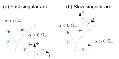
Figure 3: (Color Online) The singular arc $\alpha=0$ divides the manifold into $\alpha>0$, $\Omega_{+}$ and $\alpha<0$, $\Omega_{-}$ region. (a) The fast singular arc where the singular arc represents the optimal-time trajectory. (b) The slow singular arc where the singular arc is not the optimal-time trajectory. $X$ and $Y$ represent the $u=-1$ and $u=+1$ bang controls respectively. The insets show the behavior of $\Phi(t)\sim 0$, based on which the allowed bang-bang controls in $\Omega_{+}$ ($YX$) and $\Omega_{-}$ ($XY$) regions are indicated. The trajectory can be kept around $\alpha=0$ by alternating the $X$ and $Y$ controls.

In this subsection, we describe the general structure of the time-optimal solution in two dimension given by SussmannSussmann_87_01 ; Sussmann_87_02 ; Sussmann_87_03 . Let us consider the question: if $u(t)$ is an optimal solution, i.e., all conditions in (9) are satisfied but with a zero switching function at time $t$ (i.e., $\Phi(\boldsymbol{x}(t))=0$), what are the possible values of the dynamical variables at a later time $t+\text{d}t$? The answer relies on $\dot{\Phi}(t)$. Assume that $\mathbf{f}$ and $\mathbf{g}$ are linearly independent, their commutator can be expressed as a linear combination of $\mathbf{f}$ and $\mathbf{g}$, i.e.,

$$[\mathbf{f},\mathbf{g}]=\alpha(\boldsymbol{x})\mathbf{f}+\beta(\boldsymbol{x})\mathbf{g},$$ (37)

where $\alpha(\boldsymbol{x})$, $\beta(\boldsymbol{x})$ are smooth functions of $\boldsymbol{x}$. Time derivative of $\Phi(t)$, $\dot{\Phi}(t)$, can be computed as

$$\dot{\Phi} =\langle\boldsymbol{\lambda},[\mathbf{f},\mathbf{g}](\boldsymbol{x})\rangle$$ (38)

$$=\alpha\langle\boldsymbol{\lambda},\mathbf{f}\rangle+\beta\Phi,$$

where $\Phi=\langle\boldsymbol{\lambda},\mathbf{g}\rangle$ is used. Because $\Phi(t)=0$ and condition (10) indicates $\langle\boldsymbol{\lambda},\mathbf{f}\rangle=-|C|$, we get

$$\dot{\Phi}=-\alpha\cdot|C|.$$ (39)

Using Eq. (9d), we conclude

$$\begin{cases}\alpha>0\Rightarrow\dot{\Phi}<0&\text{allow }u=-1\text{ to }u=+1,XY\text{ control}\\ \alpha<0\Rightarrow\dot{\Phi}>0&\text{allow }u=+1\text{ to }u=-1,YX\text{ control}\end{cases}$$ (40)

Here $u=-1$ is denoted as $X$ control; $u=+1$ as $Y$ control. When $\alpha\neq 0$, $\Phi(t)=0$ can only be an isolated point in time and therefore the optimal control has to be of the bang-bang type. Eq. (40) is illustrated in Fig. 3.

The next step is to investigate if the admissible control can keep the dynamical variables along $\alpha=0$ that divides the manifold into $\alpha>0$, $\Omega_{+}$ and $\alpha<0$, $\Omega_{-}$ regions. If this happens, then $\alpha=0$ defines a singular arc along which the optimal control can be singular ($\Phi(t)=0$ over a finite amount of time); otherwise, the optimal control is of the bang-bang type. To answer this question, we consider $\alpha(\boldsymbol{x}_{0})=0$ and compute the Lie derivative of $\alpha$ with respect to the vector fields $\mathbf{X}$ and $\mathbf{Y}$. Two scenarios arise:

• (i) If $L_{\mathbf{X}}\alpha(\boldsymbol{x}_{0})$ and $L_{\mathbf{Y}}\alpha(\boldsymbol{x}_{0})$ have the same sign, then $\boldsymbol{x}_{0}$ will move out of $\alpha=0$ for all admissible controls, so $\alpha=0$ is not a singular arc.

• (ii) If $L_{\mathbf{X}}\alpha(\boldsymbol{x}_{0})$ and $L_{\mathbf{Y}}\alpha(\boldsymbol{x}_{0})$ have opposite signs, then $\alpha=0$ represents a singular arc. In this scenario, one can keep the dynamical variables around $\alpha=0$ by alternating the $X$ and $Y$ controls.

The scenario (ii) has two possible cases. Case (a): if $L_{\mathbf{X}}\alpha(\boldsymbol{x}_{0})<0,L_{\mathbf{Y}}\alpha(\boldsymbol{x}_{0})>0$, the $\alpha=0$ is the time-optimal trajectory; $\alpha=0$ is referred to as a “fast” singular arc [see Fig. 3(a)]. In this case, the optimal control is obtained by $d\alpha=0=L_{\mathbf{f}}\alpha+uL_{\mathbf{g}}\alpha$:

$$u=\frac{L_{\mathbf{X}}\alpha(\boldsymbol{x}_{0})+L_{\mathbf{Y}}\alpha(\boldsymbol{x}_{0})}{L_{\mathbf{X}}\alpha(\boldsymbol{x}_{0})-L_{\mathbf{Y}}\alpha(\boldsymbol{x}_{0})}$$ (41)

Case (b): if $L_{\mathbf{X}}\alpha(\boldsymbol{x}_{0})>0,L_{\mathbf{Y}}\alpha(\boldsymbol{x}_{0})<0$, the $\alpha=0$ is not the time-optimal trajectory; $\alpha=0$ is referred to as a “slow” singular arc [see Fig. 3(b)].

The reasoning is provided. In case (a), $\mathbf{X}$ drives $\boldsymbol{x}_{0}$ to $\Omega_{-}$ region. To go back to the singular arc, we need to apply $\mathbf{Y}$ but the $XY$ control violates the condition (40). Therefore, to move along the singular arc, PMP implies that the singular control takes the minimum time. In case (b), $\mathbf{X}$ takes $\boldsymbol{x}_{0}$ to $\Omega_{+}$ region. In $\Omega_{+}$, $XY$ control is allowed by Eq. (40), which brings the trajectory back to the singular arc. Therefore, it is not obvious if the bang-bang control or the singular control takes minimum time. It is shown that bang-bang control book:GeometricOptimalControl is the optimal solution. It may be a bit surprising that the optimal control can be determined without integrating the differential equation in time (only spatial derivatives needed), and we pinpoint that the condition $\langle\boldsymbol{\lambda},\mathbf{f}\rangle=-|C|$ leading to Eq. (39) is what makes this possible.

IV.3 The structure of optimal solutions to Grover’s problem

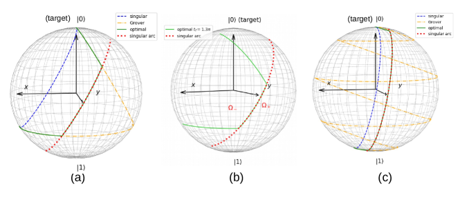
Figure 4: (Color Online) Trajectories using the singular (dashed curves), the optimal (solid curves), and Grover’s protocol (dash-dot) for (a) $x=\frac{1}{2}$ and $t_{f}=1.567\pi$, (b) $x=\frac{1}{2}$ and $t_{f}=1.3\pi$ and (c) $x=\frac{1}{4\sqrt{2}}$ and $t_{f}=5.221\pi$. The parameters of (a) and (c) are computed from Eq. (23); those of (b) are given in Fig. 2(b). In (b), $t_{f}=1.3\pi$ which is too short to reach the target state. The singular arc (dotted curves) determined by Eq. (43) is also plotted. The optimal trajectory and the singular arc coincide over a finite amount of time. The trajectory of Grover’s algorithm is zigzagging through the optimal trajectory.

The analysis provided in Section IV.2 is now applied to Eq. (35), where the two-dimensional dynamical variables are $\boldsymbol{x}=(\theta,\phi)$. The commutator $[\mathbf{f},\mathbf{g}]$ is:

$$=\left[-x\sqrt{1-x^{2}}\cot\theta\frac{1}{\sin\phi}-(1-x^{2})\frac{\cos\phi}{\sin\phi}\right]\mathbf{f}+\left[-x\sqrt{1-x^{2}}\cot\theta\frac{1}{\sin\phi}+x^{2}\frac{\cos\phi}{\sin\phi}\right]\mathbf{g}$$ (42)

$$\equiv\alpha(\theta,\phi)\mathbf{f}+\beta(\theta,\phi)\mathbf{g}.$$

The curve defined by $\alpha(\theta,\phi)=-\sqrt{1-x^{2}}(x\frac{\cot\theta}{\sin\phi}+\sqrt{1-x^{2}}\frac{\cos\phi}{\sin\phi})=0$ is

$$-\frac{x}{\sqrt{1-x^{2}}}\cot\theta=\cos\phi.$$ (43)

This curve divides the region around $\alpha=0$ into $\alpha>0$ ($\Omega_{+}$) and $\alpha<0$ ($\Omega_{-}$) regions. To identify these regions, we note that $\alpha(\frac{\pi}{2},\frac{\pi}{2})=0$, and $\alpha(\frac{\pi}{2},\frac{\pi}{2}+\epsilon)>0$, $\alpha(\frac{\pi}{2},\frac{\pi}{2}-\epsilon)<0$ (with $\epsilon$ a small positive number).

To see if $\alpha=0$ corresponds to a singular control, we compute the Lie derivative of $\alpha(\theta,\phi)$ with respect to $\mathbf{Y}$ and $\mathbf{X}$. Using $\partial_{\theta}\alpha=\frac{x\sqrt{1-x^{2}}}{\sin\phi\sin^{2}\theta}$ and $\cot\theta=-\frac{\sqrt{1-x^{2}}}{x}\cos\phi$ (the condition of $\alpha=0$), we get

$$L_{\mathbf{Y}}\alpha =\partial_{\phi}\alpha=1-x^{2}>0,$$ (44)

$$L_{\mathbf{X}}\alpha =-(1-x^{2})=-L_{\mathbf{Y}}\alpha<0.$$

Substituting Eq. (44) into Eq. (41), we see that $\alpha=0$ corresponds to a singular control with $u=0$. Fig. 4 gives the trajectories using the singular, the optimal, and Grover’s protocol for $x=1/\sqrt{4}$ and $x=1/\sqrt{32}$. Note that in Fig. 4(b) we purposely use $t_{f}=1.3\pi$ which is too short to reach the target state [see Fig. 2(b)]. The singular arc determined by Eq. (43) is also plotted. The optimal trajectory does coincide with the singular arc over a finite interval of time.

IV.4 Relation to the quantum state preparation

Although we only focus on Grover’s problem, the same technique is applicable to problems which can be reduced to a single qubit and some qualitative behaviors may provide insights into problems of higher dimensions. In this subsection we discuss two concrete examples related to the quantum state preparation.

For the Grover’s problem, the structure of singular arc and the position of the initial state (see Fig. 4) naturally introduce two critical times $T_{1}$ and $T_{2}(>T_{1})$. For the computation time $t_{f}<T_{1}$, the trajectory does not touch the singular arc and the optimal control is of bang-bang type ($Y$-$X$). $T_{2}$ is defined as the minimum time where the target state can be reached. For $T_{1}<t_{f}<T_{2}$, the optimal control is of bang-singular-bang type ($Y$-0-$X$). For $t_{f}>T_{2}$, there is no unique trajectory to reach the target state. If only the bang-bang control is allowed, there will be many switchings along the singular arc. These behaviors are found in the quantum state preparation problem (for both single-qubit and multi-qubit systems) studied in Refs. PhysRevX.8.031086 ; PhysRevLett.122.020601 . The fact that a singular control can be approximated by many bang-bang controls is reflected as the “glassy” phase (in time domain) in Refs. PhysRevX.8.031086 ; PhysRevLett.122.020601 .

For the second example, we consider the time-optimal control that steers a two-qubit product state to the fully entangled state, which is formulated and solved in Ref. PhysRevA.97.062343 . The dimension of the two-qubit Hilbert space is four. Using the symmetry of the Hamiltonian, the four-dimensional Hilbert space can be divided into two invariant subspaces and each subspace is effectively a single qubit. The formalism provided in Section II and IV.A can then be applied to one of the subspace. Without providing details, our analysis does show that the singular-bang control is the time-optimal solution as found in Ref. PhysRevA.97.062343 . One benefit of geometric control is that we are able to compute the value of the singular control [using Eq. (41)] without performing time integration.

IV.5 Analysis of Grover’s algorithm in the reduced dimension

We conclude this section by analyzing Grover’s algorithm in the $(\theta,\phi)$ manifold, where the problem is to steer the dynamical variables from $(\theta_{i},\phi_{i})=(2\arctan\frac{\sqrt{1-x^{2}}}{x},0)$ to $\theta_{f}=0$. We first note that by substituting $\tan\theta_{i}=\frac{\sqrt{1-x^{2}}}{x}$ and $\phi_{i}=0$ into Eq. (34a), one gets $\mathbf{X}(\theta_{i},\phi_{i})=0$. This indicates that the $X$ ($u=-1$) control cannot change the initial dynamical variables $(\theta_{i},\phi_{i})$ and the bang control has to start with $Y$ ($u=+1$). Next, we notice that only one of the bang controls, the $X$ control, can change the value of $\theta$. To drive $\theta$ from $\theta_{i}$ to 0 with a minimum number of bang-to-bang switchings, we need to maximize the reduction of $\theta$ during the $X$ control. To obtain the maximum $\theta$-reduction, we consider the dynamics with the $X$ control given in Eq. (34a):

$$\frac{\text{d}\theta}{\text{d}t} =-2x\sqrt{1-x^{2}}\sin\phi,$$ (45a)

$$\frac{\text{d}\phi}{\text{d}t} =(2x^{2}-1)-2x\sqrt{1-x^{2}}\cos\phi\cot\theta.$$ (45b)

For small $x$, $x\cot\theta\leq 1/N$ holds for $\theta\in[Nx,\pi-Nx]$ (one can pick $N=10$), indicating $\frac{\text{d}\phi}{\text{d}t}\approx-1$ [Eq. (45b)] over this range. Integrating Eq. (45a) from $\phi_{i}$ to $\phi_{f}$ with $\frac{\text{d}\phi}{\text{d}t}\approx-1$, we get the change of $\theta$ as

$$\Delta\theta =-2x\sqrt{1-x^{2}}\int_{\phi_{i}}^{\phi_{f}}\sin\phi\frac{\text{d}t}{\text{d}\phi}\text{d}\phi$$ (46)

$$\approx 2x\sqrt{1-x^{2}}\left[\cos\phi_{i}-\cos\phi_{f}\right]$$

$$\geq 2x\sqrt{1-x^{2}}\left[-2\right]\equiv-|\Delta\theta|_{\text{max}}$$

The maximum $\theta$-reduction $|\Delta\theta|_{\text{max}}=4x\sqrt{1-x^{2}}$ can only be obtained when $\phi_{i}=\pi$ and $\phi_{f}=0$. To achieve $|\Delta\theta|_{\text{max}}$ from $\phi_{i}=0$, one first (a) applies $Y$ ($\mathbf{Y}=\partial_{\phi}$) control for time $\pi$ that takes $\phi$ from 0 to $\pi$, and then (b) applies $X$ ($\mathbf{X}\approx-2x\sin\phi\partial_{\theta}-\partial_{\phi}$ for small $x$) control for time $\pi$ that takes $\phi$ from $\pi$ back to 0; it is (b) that reduces the $\theta$ by $|\Delta\theta|_{\text{max}}$. (a) and (b) will be repeated $N$ times to bring $\theta=\theta_{i}$ to $\theta=0$. For small $x$, $\theta_{i}\approx\pi$ and $N$ is estimated as

$$\frac{\theta_{i}}{|\Delta\theta|_{\text{max}}}\approx\frac{\pi}{4x}.$$ (47)

This procedure is identical to Grover’s algorithm described in Section III.1. We conclude that in terms of optimal control, Grover’s algorithm uses the bang-bang protocol with a minimum number of switchings to approximate the optimal bang-singular-bang control. To visualize this point, in Fig. 4(c) we show that the trajectory of Grover’s algorithm is zigzagging through the optimal trajectory. Cutting the number of switchings reduces the query complexity, which is how the quantum speedup is defined in quantum computation using a discrete sequence of gates.

V Conclusion

Grover’s quantum search problem is one of the most well known and important problems in quantum computation. In this paper, we formulate this problem as a time-optimal control problem, and apply Pontryagin’s Minimum Principle to solve it. Designing a quantum algorithm is equivalent to solving a time-optimal control problem where the dynamical variables are the components of the wave function, the dynamics are the specified by the Schrödinger’s equation, and the target state is the ground state of the given “problem Hamiltonian”. Although the dimension of the Hilbert space of Grover’s problem can be arbitrarily large, it can be reduced to a two-dimensional Schrödinger equation. We show that the optimal control for Grover’s problem has the bang-singular-bang structure and explicitly demonstrate that the optimal protocol does take shorter time to reach the target state when comparing to other known protocols. This bang-singular-bang can be derived without integrating the differential equations by using geometric control technique. The key step is to derive the dynamical equations involving only two real-valued dynamical variables. Within this manifold, applying geometric control provides the optimal protocol at each point. The formalism provided in this paper can be beneficial to any quantum systems which can be effectively described by a single qubit. We are aware that the generalization to systems of higher dimensions may not be as informative as the analysis relies on enumerating all possibilities, but can be worth investigating. The key insight brought by time-optimal control theory is that in addition to the bang-bang protocol the singular control should be considered. However, PMP provides an efficient and exact formalism to compute the gradient of the cost function at a given control, which can be useful in numerical optimization for problems of higher dimensions. In view of optimal control, Grover’s algorithm uses bang-bang protocol, with a minimum number of bang-to-bang switchings to reduce the query complexity, to approximate the optimal protocol. Our work provides a concrete example how optimal control is connected to the quantum computation, and may shed some light on how a quantum algorithm can be designed.

Appendix A Operator as a vector field in $(\theta,\phi)$

In this appendix, Eq. (32) that relates the vector fields defined on the tangent space of $(\theta,\phi)$ to the Pauli matrices are derived. Applying $H=\sigma_{z}$ on a state $|\Psi(\theta,\phi)\rangle$ over a time interval $dt$, we get

$$e^{-i\sigma_{z}\cdot\text{d}t}\begin{bmatrix}\cos\frac{\theta}{2}\\ \sin\frac{\theta}{2}e^{i\phi}\end{bmatrix}=\begin{bmatrix}\cos\frac{\theta}{2}e^{-i\,\text{d}t}\\ \sin\frac{\theta}{2}e^{i(\phi+\text{d}t)}\end{bmatrix}\rightarrow\begin{bmatrix}\cos\frac{\theta}{2}\\ \sin\frac{\theta}{2}e^{i(\phi+2\,\text{d}t)}\end{bmatrix}.$$ (48)

After forcing the first component to be real and positive, $e^{-i\sigma_{z}\cdot\text{d}t}$ only changes the $\phi$ component. We therefore conclude $\sigma_{z}\rightarrow 2\partial_{\phi}$.

Applying $H=\sigma_{x}$ on a state $|\Psi(\theta(0),\phi(0))\rangle$ over a time interval $dt$, we get

$$e^{-i\sigma_{x}\cdot\text{d}t}\begin{bmatrix}\cos\frac{\theta(0)}{2}\\ \sin\frac{\theta(0)}{2}e^{i\phi(0)}\end{bmatrix}=\begin{bmatrix}1&-i\,\text{d}t\\ -i\,\text{d}t&1\end{bmatrix}\begin{bmatrix}\cos\frac{\theta(0)}{2}\\ \sin\frac{\theta(0)}{2}e^{i\phi(0)}\end{bmatrix}$$ (49)

$$= \begin{bmatrix}\cos\frac{\theta(0)}{2}+\text{d}t\,\sin\frac{\theta(0)}{2}\sin\phi(0)-i\,\text{d}t\,\sin\frac{\theta(0)}{2}\cos\phi(0)\\ \sin\frac{\theta(0)}{2}e^{i\phi(0)}-i\,\text{d}t\cos\frac{\theta(0)}{2}\end{bmatrix}\rightarrow\begin{bmatrix}\cos\frac{\theta(\text{d}t)}{2}\\ \sin\frac{\theta(\text{d}t)}{2}e^{i\phi(\text{d}t)}\end{bmatrix}.$$

Applying $\sigma_{x}$ changes both $\theta$ and $\phi$ components. We note that $A+i\,\text{d}t=A(1+i(\text{d}t/A))\sim Ae^{i\text{d}t/A}$, so to the first order a small imaginary part does not change the amplitude. For the first component, we see that

$$\cos\frac{\theta(\text{d}t)}{2}=\cos\frac{\theta(0)}{2}+\text{d}t\,\sin\frac{\theta(0)}{2}\sin\phi(0)$$ (50)

$$\Rightarrow \frac{\text{d}\theta}{\text{d}t}=-2\sin\phi.$$

The amplitude change of the first component determines the coefficient of $\partial_{\theta}$. The first component also introduces a phase term $1-i\,\text{d}t\,\tan\frac{\theta(0)}{2}\cos\phi(0)$ which has to be compensated. Therefore, the second component gives

$$\sin\frac{\theta(\text{d}t)}{2}e^{i\phi(\text{d}t)}=\left[\sin\frac{\theta(0)}{2}e^{i\phi(0)}-i\,\text{d}t\cos\frac{\theta(0)}{2}\right]\left[1+i\,\text{d}t\,\tan\frac{\theta(0)}{2}\cos\phi(0)\right]$$ (51)

$$\Rightarrow \sin\frac{\theta(\text{d}t)}{2}e^{i\phi(\text{d}t)}-\sin\frac{\theta(0)}{2}e^{i\phi(0)}=i\,\text{d}t\left[\sin\frac{\theta(0)}{2}\tan\frac{\theta(0)}{2}\cos\phi(0)e^{i\phi(0)}-\cos\frac{\theta(0)}{2}\right]$$

$$\Rightarrow \frac{1}{2}\cos\frac{\theta}{2}\frac{\text{d}\theta}{\text{d}t}+\sin\frac{\theta}{2}i\frac{\text{d}\phi}{\text{d}t}=i\left[\sin\frac{\theta}{2}\tan\frac{\theta}{2}\cos\phi-\cos\frac{\theta}{2}\,e^{-i\phi}\right].$$

Using $\frac{\text{d}\theta}{\text{d}t}=-2\sin\phi$ and $e^{-i\phi}=\cos\phi-i\sin\phi$, we get

$$-\cos\frac{\theta}{2}\sin\phi+i\sin\frac{\theta}{2}\frac{\text{d}\phi}{\text{d}t}=i\left[\sin\frac{\theta}{2}\tan\frac{\theta}{2}\cos\phi-\cos\frac{\theta}{2}\,(\cos\phi-i\sin\phi)\right]$$ (52)

$$\Rightarrow \frac{\text{d}\phi}{\text{d}t}=\cos\phi\left[\tan\frac{\theta}{2}-\cot\frac{\theta}{2}\right]=-2\cos\phi\cot\theta.$$

Combining Eq. (50) and  (52), we get

$$\sigma_{y}\rightarrow-2\sin\phi\partial_{\theta}-2\cos\phi\cot\theta\partial_{\phi}.$$ (53)

The vector field corresponding to $\sigma_{y}$ can be derived similarly. A straightforward calculation gives

$$n_{x}\sigma_{x}+n_{z}\sigma_{z} \rightarrow n_{x}V_{x}+n_{z}V_{z}=-2n_{x}\sin\phi\,\partial_{\theta}+2\left[n_{z}-n_{x}\cos\phi\cot\theta\right]\partial_{\phi},$$ (54)

which is useful to map Hamiltonians appeared in Grover’s problem to their corresponding vector fields.

References

- (1) Michael A. Nielsen and Isaac L. Chuang. Quantum Computation and Quantum Information. Cambridge University Press, 2011.
- (2) Michele Mosca Phillip Kaye, Raymond Laflamme. An introduction to quantum computing. Oxford University Press, USA, 2007.
- (3) Peter W. Shor. Polynomial-time algorithms for prime factorization and discrete logarithms on a quantum computer. SIAM J. Comput., 26(5):1484–1509, October 1997.
- (4) Lov K. Grover. A fast quantum mechanical algorithm for database search. In Proceedings of the Twenty-eighth Annual ACM Symposium on Theory of Computing, STOC ’96, pages 212–219, New York, NY, USA, 1996. ACM.
- (5) Lov K. Grover. Quantum mechanics helps in searching for a needle in a haystack. Phys. Rev. Lett., 79:325–328, Jul 1997.
- (6) David Deutsch and Richard Jozsa. Rapid solution of problems by quantum computation, Mar 1992.
- (7) Daniel R. Simon. On the power of quantum computation. SIAM J. Comput., 26(5):1474–1483, October 1997.
- (8) C. Bennett, E. Bernstein, G. Brassard, and U. Vazirani. Strengths and weaknesses of quantum computing. SIAM Journal on Computing, 26(5):1510–1523, 1997.
- (9) Aram W. Harrow, Avinatan Hassidim, and Seth Lloyd. Quantum algorithm for linear systems of equations. Phys. Rev. Lett., 103:150502, Oct 2009.
- (10) Edward Farhi and Sam Gutmann. Analog analogue of a digital quantum computation. Phys. Rev. A, 57:2403–2406, Apr 1998.
- (11) Tadashi Kadowaki and Hidetoshi Nishimori. Quantum annealing in the transverse ising model. Phys. Rev. E, 58:5355–5363, Nov 1998.
- (12) Edward Farhi, Jeffrey Goldstone, Sam Gutmann, Joshua Lapan, Andrew Lundgren, and Daniel Preda. A quantum adiabatic evolution algorithm applied to random instances of an np-complete problem. Science, 292(5516):472–475, 2001.
- (13) Jérémie Roland and Nicolas J. Cerf. Quantum search by local adiabatic evolution. Phys. Rev. A, 65:042308, Mar 2002.
- (14) Edward Farhi, Jeffrey Goldstone, Sam Gurmann, and Michael Sipser. Quantum computation by adiabatic evolution, 2000.
- (15) A. T. Rezakhani, W.-J. Kuo, A. Hamma, D. A. Lidar, and P. Zanardi. Quantum adiabatic brachistochrone. Phys. Rev. Lett., 103:080502, Aug 2009.
- (16) Quntao Zhuang. Increase of degeneracy improves the performance of the quantum adiabatic algorithm. Phys. Rev. A, 90:052317, Nov 2014.
- (17) H. F. Trotter. On the product of semi-groups of operators. Proceedings of the American Mathematical Society, 10, 1959.
- (18) Masuo Suzuki. Generalized trotter’s formula and systematic approximants of exponential operators and inner derivations with applications to many-body problems. Communications in Mathematical Physics, 51(2):183–190, Jun 1976.
- (19) J. Brooke. Quantum annealing of a disordered magnet. Science, 284, 4 1999.
- (20) Erio Santoro, Giuseppe E; Tosatti. Optimization using quantum mechanics: quantum annealing through adiabatic evolution. Journal of Physics A: Mathematical and General Physics, 39, 09 2006.
- (21) Arnab Das and Bikas K. Chakrabarti. Colloquium: Quantum annealing and analog quantum computation. Rev. Mod. Phys., 80:1061–1081, Sep 2008.
- (22) M W Johnson, P Bunyk, F Maibaum, E Tolkacheva, A J Berkley, E M Chapple, R Harris, J Johansson, T Lanting, I Perminov, E Ladizinsky, T Oh, and G Rose. A scalable control system for a superconducting adiabatic quantum optimization processor. Superconductor Science and Technology, 23(6):065004, apr 2010.
- (23) Damian S. Steiger, Troels F. Rønnow, and Matthias Troyer. Heavy tails in the distribution of time to solution for classical and quantum annealing. Phys. Rev. Lett., 115:230501, Dec 2015.
- (24) Bettina Heim, Troels F. Rønnow, Sergei V. Isakov, and Matthias Troyer. Quantum versus classical annealing of ising spin glasses. Science, 348(6231):215–217, 2015.
- (25) Alberto Peruzzo, Jarrod McClean, Peter Shadbolt, Man-Hong Yung, Xiao-Qi Zhou, Peter J. Love, Alań Aspuru-Guzik, and Jeremy L. O’Brien. A variational eigenvalue solver on a photonic quantum processor. Nature Communications, 5:4213, 2014.
- (26) P. J. J. O’Malley, R. Babbush, I. D. Kivlichan, J. Romero, J. R. McClean, R. Barends, J. Kelly, P. Roushan, A. Tranter, N. Ding, B. Campbell, Y. Chen, Z. Chen, B. Chiaro, A. Dunsworth, A. G. Fowler, E. Jeffrey, E. Lucero, A. Megrant, J. Y. Mutus, M. Neeley, C. Neill, C. Quintana, D. Sank, A. Vainsencher, J. Wenner, T. C. White, P. V. Coveney, P. J. Love, H. Neven, A. Aspuru-Guzik, and J. M. Martinis. Scalable quantum simulation of molecular energies. Phys. Rev. X, 6:031007, Jul 2016.
- (27) Antonio; Temme Kristan; Takita Maika; Brink Markus; Chow Jerry M.; Gambetta Jay M. Kandala, Abhinav; Mezzacapo. Hardware-efficient variational quantum eigensolver for small molecules and quantum magnets. Nature, 549, 9 2017.
- (28) Edward Farhi, Jeffrey Goldstone, and Sam Gurmann. A quantum approximate optimization algorithm, 2014.
- (29) Dave Wecker, Matthew B. Hastings, and Matthias Troyer. Progress towards practical quantum variational algorithms. Phys. Rev. A, 92:042303, Oct 2015.
- (30) Han-Hsuan Lin Cedric Yen-Yu Lin. Performance of qaoa on typical instances of constraint satisfaction problems with bounded degree, 2016.
- (31) John Preskill. Quantum Computing in the NISQ era and beyond. Quantum, 2:79, August 2018.
- (32) Nanyang Xu, Jing Zhu, Dawei Lu, Xianyi Zhou, Xinhua Peng, and Jiangfeng Du. Quantum factorization of 143 on a dipolar-coupling nuclear magnetic resonance system. Phys. Rev. Lett., 108:130501, Mar 2012.
- (33) Cedric Yen-Yu Lin Han-Hsuan Lin Peter Shor Elizabeth Crosson, Edward Farhi. Different strategies for optimization using the quantum adiabatic algorithm, 2014.
- (34) Dave Wecker, Matthew B. Hastings, and Matthias Troyer. Training a quantum optimizer. Phys. Rev. A, 94:022309, Aug 2016.
- (35) David G. Luenberger. Introduction to dynamic systems: theory, models, and applications. Wiley, 1979.
- (36) Daniel Liberzon. Calculus of Variations and Optimal Control Theory: A Concise Introduction. Princeton University Press, 2012.
- (37) Urszula Ledzewicz Heinz Schattler. Geometric Optimal Control: Theory, Methods and Examples. Interdisciplinary Applied Mathematics 38. Springer-Verlag New York, 1 edition, 2012.
- (38) L. S. Pontryagin. Mathematical Theory of Optimal Processes. CRC Press, Boca Raton, FL, 1987.
- (39) Seraph Bao, Silken Kleer, Ruoyu Wang, and Armin Rahmani. Optimal control of superconducting gmon qubits using pontryagin’s minimum principle: Preparing a maximally entangled state with singular bang-bang protocols. Phys. Rev. A, 97:062343, Jun 2018.
- (40) Zhi-Cheng Yang, Armin Rahmani, Alireza Shabani, Hartmut Neven, and Claudio Chamon. Optimizing variational quantum algorithms using pontryagin’s minimum principle. Phys. Rev. X, 7:021027, May 2017.
- (41) Junkai Zeng and Edwin Barnes. Fastest pulses that implement dynamically corrected single-qubit phase gates. Phys. Rev. A, 98:012301, Jul 2018.
- (42) Guang Hao Low, Theodore J. Yoder, and Isaac L. Chuang. Quantum imaging by coherent enhancement. Phys. Rev. Lett., 114:100801, Mar 2015.
- (43) Guang Hao Low and Isaac L. Chuang. Optimal hamiltonian simulation by quantum signal processing. Phys. Rev. Lett., 118:010501, Jan 2017.
- (44) Marin Bukov, Alexandre G. R. Day, Dries Sels, Phillip Weinberg, Anatoli Polkovnikov, and Pankaj Mehta. Reinforcement learning in different phases of quantum control. Phys. Rev. X, 8:031086, Sep 2018.
- (45) Alexandre G. R. Day, Marin Bukov, Phillip Weinberg, Pankaj Mehta, and Dries Sels. Glassy phase of optimal quantum control. Phys. Rev. Lett., 122:020601, Jan 2019.
- (46) Note that the conventional Hamiltonian is given by with . To be consistent with the convention in control thoery, we define and such that .
- (47) H. J. Sussmann. The structure of time-optimal trajectories for single-input systems in the plane: The non-singular case. SIAM Journal on Control and Optimization, 25:433, 1987.
- (48) H. J. Sussmann. The structure of time-optimal trajectories for single-input systems in the plane: The general real analytic case. SIAM Journal on Control and Optimization, 25:868, 1987.
- (49) H. J. Sussmann. Regular synthesis for time-optimal control of single-input real analytic systems in the plane. SIAM Journal on Control and Optimization, 25:1145, 1987.