Dark matter from dark photons:
a taxonomy of dark matter production
Abstract
We analyse how dark matter (DM) can be produced in the early universe, working in the framework of a hidden sector charged under a U(1)’ gauge symmetry and interacting with the Standard Model through kinetic mixing. Depending on the masses of the dark matter particle and of the dark photon, as well as on the hidden U(1)’ gauge coupling and the kinetic mixing parameter, we classify all the distinct regimes along which the observed dark matter relic density can be accounted for. We find that 9 regimes are potentially operative to produce the DM particles and this along 5 distinct dynamical mechanisms. Among these, 4 regimes are new and correspond to regimes in which the DM particles are produced by on-shell dark photons. One of them proceeds along a new dynamical mechanism, which we dub sequential freeze-in. We argue that such regimes and the associated dynamical mechanisms are characteristic of DM models for which, on top of the Standard Model and the dark sector, there are other massive, but relatively light particles — akin to the dark photon — that interact both with the SM and the DM sectors.
I Introduction
As the nature of the dark matter (DM) remains a mystery, it is possible that DM is a particle that belongs to a whole new hidden sector. This hidden sector may be coupled through the Standard Model (visible sector) through a few possible portals Patt:2006fw . The question we study further in the present work is how to account, in generic terms, for the abundance of a dark matter (DM) particle produced through portals. For the case of the kinetic mixing portal with a massless dark photon, this has been addressed in much details Chu:2011be . That work also includes the case of dark matter creation through the Higgs portal. In the present work, we consider the possible impact of a finite dark photon mass. More generically, our study applies to DM production in models in which a relatively light particle couples both to the DM and to SM particles.
The existence of a massive dark photon, associated to a hidden U(1)’ gauge interaction, has been the object of many investigations, both theoretically and experimentally, see e.g. the reviews Jaeckel:2010ni ; Essig:2013lka ; Alexander:2016aln . This possibility is well-motivated, very rich phenomenologically and, moreover, is directly related to the DM problem. Indeed, a gauge symmetry is a most natural way to stabilize a particle Foot:2014uba ; Ackerman:mha ; Feng:2008mu ; Feng:2009mn ; Hambye:2010zb . Specifically, we consider the following simple and popular model
| (1) | |||||
Here is a Dirac fermion, singlet under the SM gauge group but charged under U(1)’ and will be our DM candidate. Its covariant derivative is , where and are the U(1)’ gauge field and coupling. This dark, or hidden, sector is coupled to the Standard Model (SM) sector through the so-called kinetic mixing portal term, which mixes the dark gauge field to the SM hypercharge one with a mixing parameter Holdom:1985ag . This Lagrangian thus involves 4 new parameters, , , and what will turn out to be the mass of the dark photon particle, . Equivalently, we will make use of the hidden sector fine structure constant and of the combination , which is the millicharge of the DM in the limit . The dark photon mass can arise either through the Stückelberg Stueckelberg:1900zz or through the Brout-Englert-Higgs mechanism Englert:1964et ; Higgs:1964pj . In the latter case, there are necessarily several other parameters and degrees of freedom associated to U(1)’ breaking (the dots in Eq. (1)). In the sequel, we will assume that these extra ingredients may be neglected. However, we will briefly discuss their possible impact in Appendix B.
In the case of a massless dark photon, the problem of accounting for the DM abundance through the kinetic mixing portal has been studied in Chu:2011be . It has been shown in that work that the observed relic density could be reached along 4 distinct dynamical mechanisms depending on the values of the parameters of the model. These dynamical mechanisms are: freeze-in (regime Ia in the sequel) McDonald:2001vt ; Hall:2009bx ; Chu:2011be ; Bernal:2017kxu , reannihilation (IIIa) Hall:2009bx ; Chu:2011be , secluded freeze-out (IVa)111By secluded freeze-out, we refer here to a scenario in which DM particles freeze-out in the dark sector Pospelov:2007mp ; Pospelov:2008zw but with a temperature different from the temperature of the SM visible sector, as in Chu:2011be ; Feng:2009mn . and, finally, the standard text-book thermal freeze-out mechanism (Va and Vb). Altogether, these 4 mechanisms lead to 5 different regimes through which the DM abundance can be reached in the case of a massless dark photon. Indeed, the standard freeze-out of the dark matter particles could occur either through annihilation into SM particles (Vb regime) or into the dark photons themselves (Va regime). We will thus distinguish production mechanisms (classified using Roman numerals) and regimes (distinguished using the Latin letter a or b, as in the case of freeze-out).
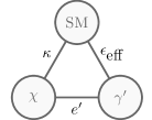
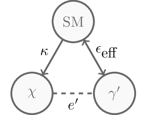
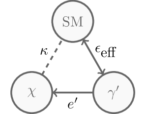
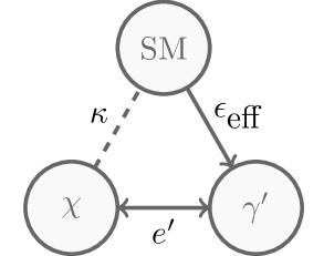
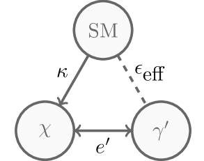
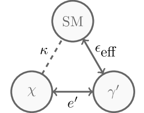
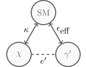
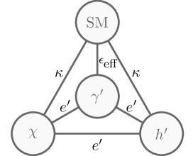
The aim of the present work is to revisit this classification of DM production mechanisms, taking into account the possible effects of the mass of the dark photon. By considering the dark photon model above, the generic underlying structure we will be considering is that of a system composed of 3 distinct particle sectors, together with 3 possible connections between the sectors. This structure is depicted in Fig. 1, again with a focus on the kinetic mixing setup and its ingredients. So, the 3 sectors (depicted as blobs) consist of the SM, the dark matter particle and the massive dark photon , while the connections between the sectors (depicted as lines) are parameterized by the mixing (or more precisely , which will be defined below), the hidden fine structure constant and the ”millicharge” . Considering such a structure, we will point out the existence of 4 new regimes (noted Ib, II, IIIa and IVa), including one along a new dynamical mechanism (II), making in total potentially 9 distinct ways to reach the observed DM abundance.
As we will explain in the following sections, the 9 production regimes can be read from this figure by considering the different ways through which the hidden sector particles can be created and whether they are in thermal equilibrium with each others and/or with the SM sector. This is shown in Fig. 2. There, one sees the 4 new regimes that emerge in the case of massive dark photon (and so are absent in the massless limit — see later) and noted Ib, II, IIIa and (a priori, see however below) IVa. As the solid arrow lines between the sectors mean to suggest, they all correspond to regimes in which DM is created from the SM sector via the production of real, on mass-shell dark photons. All these regimes follow each others along a characteristic pattern in the parameter space, which in the sequel we call ”the phase diagram” and that can be seen in Figs. 4 and 5 for two illustrative hidden sector mass setups. Most interestingly, some of these new regimes allow for DM production for values of that are even smaller than in the case of standard freeze-in (regime Ia). As we will see, whether a specific regime is actually relevant will depend not only on the connections parameters, but also on the DM and dark photon masses.
Our work is organized as follows. In Section II we will present how the various particles in the kinetic portal model of (1) can interact, focusing on the case of a massive dark photon. Next, in Section III we will derive and discuss the parameter space or phase diagram in which we show, as a function of the parameters, how the different regimes that lead to the observed DM relic density are related with each others. We discuss each regime in details but put a particular emphasis on the new regimes. For the sake of our classification and to simplify our discussion, in that section we will be putting aside some complications that arise due to the peculiar nature of the kinetic mixing portal. In particular, we neglect there the impact of thermal effects on the propagation and production of dark photons. These will be considered in Section IV, emphasizing their impact on the different production regimes we found. Next we will discuss briefly, in Section V, the other constraints which hold on this model. Finally, in Section VI, we will elaborate on the generality of the phase diagram we have obtained, discussing the possible effect of other degrees of freedom and then draw our conclusions. The Appendix A contains a technical summary based on the existing literature on thermal effects on dark photons production and progagation. The case in which the mass of the dark photon arise through the Brout-Englert-Higgs mechanism is considered in Appendix B.
II The three sectors and their connections
We focus on the model of Eq. (1) and aim at studying the abundance of the new particles, here the dark matter, made of particle and , and the dark photon . To determine the relevant processes, we need to establish the coupling of dark photons to the SM sector. The procedure is standard and consists first to have canonical kinetic terms for the gauge fields; we repeat the argument here for the sake of clarity. To do so, we exploit the fact that the values of that are relevant for DM production will turn out to be always small numbers, so we can treat the effects of mixing as a perturbation. From Eq. (1), making the non-orthogonal transformation
| (2) |
leads to
| (3) | |||||
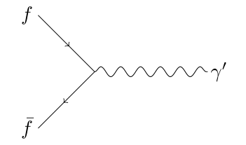
to leading order in , where we only show the terms relevant for our argument. Clearly, as the SM particles only couple to the SM gauge fields, in particular the neutral ones, and , in the limit , they do not mix with the dark photon . Here is the usual Weinberg angle; the subscript is to insist on the fact that they are the usual SM fields. The SM particles do not interact with the dark photon while the particles are coupled to the SM photon with millicharge , where . They are also coupled vectorially to the boson, with coupling . Thus, if , the only possibility to create dark photons is through the production of particles Foot:1994bx ; Chu:2011be .
If, on the other hand, , dark photons can be created directly by SM particles through the mixing mass term
| (4) |
in Eq. (3). Like in the description of neutrino oscillations, we refer to the basis of Eq. (3) as the interaction eigenstates basis. It is interesting to go forward and diagonalize the mass terms. We will only consider cases in which , and so again we do the diagonalization to leading order in . Performing the orthogonal transformation
| (5) |
transforms Eq. (4) into
| (6) |
while , with like in the SM. Now, it is easy to see that this mixing term introduces a mass splitting between the and field that is and thus can be neglected. So the dark photon field has indeed a mass
| (7) |
while the field is massless. This eigenmass basis makes clear that the particles couple only to the massive dark photon and to the SM boson, and not to the massless photon, a fact that is well-known,
| (8) |
(we drop the subscript on the field from now on as ). Also, the electrically charged SM particles, like the electron, couple to the dark photon with coupling
| (9) |
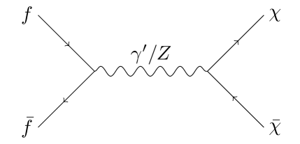
In the model just introduced we must thus consider the existence of three distincts populations (or sectors, or reservoirs) of particles in the early stages of the universe. The main reservoir consists of the SM particles; they will be assumed to be in thermal equilibrium at a temperature . The hidden sector consists on one side of the particles and their antiparticles (DM) and, on the other side, of the dark photons. These two populations do not have to be necessarily in thermal equilibrium with each others or with the SM sector. Their respective abundance depends then on how the 3 reservoirs are connected with each others. The dominant processes directly connecting the SM and DM populations are pair annihilation of SM particles (or boson decay for some mass range) into DM pairs Chu:2011be . The strength of these processes is essentially set by a single parameter (the ”millicharge”),
| (10) |
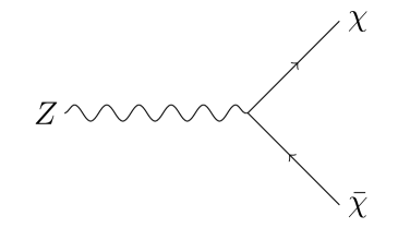
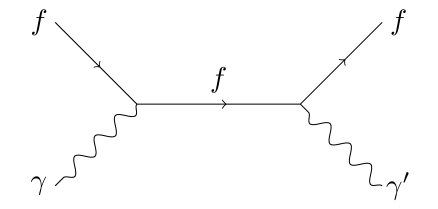
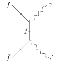
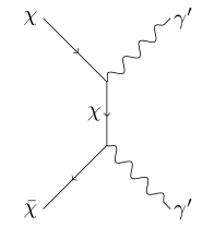
The processes connecting the SM reservoir and the dark photon population are on the other hand determined by the parameter; these a priori include Bremsstrahlung (which may be neglected), Compton scattering , pair annihilation , and coalescence . They involve distinct powers of but also distinct temperature dependence and so are dominant in different mass and temperature regimes. As for the processes connecting the DM and dark photon populations, they are set by and are dominated (at lowest order in ) by . The Feynman diagrams for all these connecting processes are shown in Fig. 3.
This structure leads to the diagram of Fig. 1, where the blobs represent schematically the reservoirs and the lines the possible connections. In the massless case the triangle of Fig. 1 has one connecting edge less since there is no direct connection between the hidden photon and SM populations. This, in brief, explains why there are more DM production regimes in the massive case than in the massless case.
III Phase diagram of dark matter production
We now turn to the systematic discussion of the dependence of the DM relic abundance on the connector parameters, starting from an empty reservoir in the dark sector, passing through all the regimes, up to a dark sector that is fully in thermal equilibrium with the SM. For the sake of clarity and generality, we will not include in this section any of the thermal effects that are specific to the dark photon setup. Instead, thermal effects on dark photon production, which can be very important in some cases as we shall see, will be determined and discussed in Section IV. Also, in this section and the sequel, we will rely heavily on the results obtained in Ref. Chu:2011be , to which we refer for more in-depth discussions of some of the production regimes, including explicit expressions for the relevant cross-sections (given in that reference for a massless dark photon).
The DM abundance depends on the DM and dark photon masses and two among the three connector parameters , and , since only two are independent, see Eq. (10). Thus, for a given set of and masses, one can for instance give the relic abundance as contour lines in the plane. This representation leads to a “phase diagram” that displays the various regimes. Note importantly that for all the discussion below we will always assume that so that DM is always kinematically free to annihilate into dark photons. The opposite case leads to a different (and simpler) phenomenology that we will not discuss here. The phase diagram comes out from integrating a set of Boltzmann equations that determine the evolution of the DM and yields as function of the visible sector temperature. For the case of a massless dark photon, the contour lines of constant DM relic density in the phase diagram have roughly the shape of a rectangle (dubbed the “mesa” in Chu:2011be ), displaying 5 regimes, along 4 dynamical production mechanisms. These 4 mechanisms are freeze-in (Ia in the classification of Fig. 2), reannihilation (IIIb), secluded freeze-out (IVb) and ordinary freeze-out (with freeze-out either to dark photons, Va, or SM particles, Vb, leading all together to 5 distinct regimes). Starting with an empty hidden sector, the DM abundance is reached through the following sequence of regimes
| (11) |
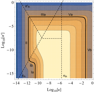
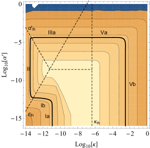
In particular, the freeze-in regime, Ia, proceeds through slow driven processes and leads to a vertical line at small in the ”mesa” structure of the phase diagram, see Chu:2011be . When the dark photon mass matters, this simple vertical line structure does not hold anymore and instead one has a more complicated structure for small . Actually, one can distinguish 4 more regimes for values of that are small enough so that the processes do not thermalize. This is illustrated by the phase diagram depicted in Fig. 4 which we get for one example set of masses, GeV and GeV. Much heavier DM candidates are of course possible, as shown in Fig. 5, for GeV and GeV. More to the point, the phase diagram, which shows contour lines of constant DM relic density, has a distinct shape: the ”mesa” has an extension toward much smaller value of the parameter, suggesting the shape of a “mooring bollard”. These features, and the corresponding new regimes, are, as we shall see, due to the possibility of dark photon production of DM.
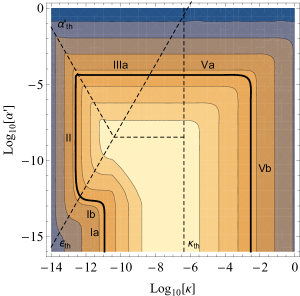
The most generic sequence of regimes appearing along the mooring bollard pattern is the one appearing in Figs. 4 and 5, that is to say
| (12) |
This structure, on top of the regimes already existing in the massless case (Ia, Va and Vb), involve 3 new regimes: Ib, II and IIIa. The fourth new regime, IVa, as well as the 2 other regimes already existing in the massless case (IIIb and IVb), can appear for other choices of the parameter and more generally for other models. The four new regimes arise from the extra SM production of dark photons. In all cases the mooring bollard shape of the phase diagram is a generic signature.
The general set of Boltzmann equations that determine the evolution of the DM and abundances (, with the entropy density and ) as a function of time, and so that leads to the phase diagram, takes the form222Here and in subsequent Boltzmann equations, we have included factors of , typical of Dirac DM particles, into the definitions of the cross-sections Gondolo:1990dk .
| (13) | |||||
| (14) | |||||
where is the Hubble parameter and , with the temperature of the visible sector. The quantity refers to the decay rate into a pair of DM particles. In writing these Boltzmann equations, we assumed that the dark photon is lighter than the dark matter (excluding for instance the channel ). A sum over the different and channels is implicit everywhere in these equations. In the sequel, so as to avoid cluttering of the equations, we will regroup the scattering and decay terms involving SM particles into
| (15) |
and
| (16) |
Although the Boltzmann equations contain many terms, for most production regimes, only one or two of these terms are relevant. As we will see too, these equations are not sufficient to correctly determine the amount of DM produced in the reannihilation regimes, which are characterized by a hidden and visible sectors with distinct temperatures: in these cases, one also needs to evaluate the energy that has been transferred from the SM to the hidden sector particles.
To understand the distinction between the various production regimes, it is useful to start by delimiting the regions of parameter space depending on whether the various connecting processes lead, or not, to thermalization. To determine whether the DM particles thermalize with the SM thermal bath, we take the simple criteria
| (17) |
with . This leads to the following condition on the millicharge parameter,
| (18) |
which is depicted by a vertical line in Figs. 4 and 5. As for the thermalization of the dark photons with the SM thermal bath, what matters typically is if thermalization (which leads to ) has occurred by the time when the DM number freezes, . Thus similarly to the condition above, we use
| (19) |
as the condition for the thermalization of the dark photons with the SM, which numerically translates in a condition on the (in principle effective, but we remind the reader that we neglect the thermal effect for the time being) mixing parameter,
| (20) |
with . As , this condition corresponds to a diagonal dashed line in the phase diagram, see Figs. 4 and 5. As for the thermalization between the dark photons and DM particles themselves, it depends on the scenario considered. We now discuss each of the new regimes, using the phase diagram of Fig. 4 as reference.
III.1 Freeze-in: regimes Ia and Ib
The Ia freeze-in regime corresponds to production of DM particles directly from the SM particles, through out-of-equilibrium processes parameterized by . In this regime, is assumed to be too small for the processes to play any role. Thus, in Eq. (13) only the term is relevant for producing the DM.
| (21) |
For fixed DM mass, the production depends only on the parameter so the observed relic abundance is given by a vertical line in the phase diagram, corresponding to the lower left corner in Fig. 4.
Note that for small value of , and with the value of that this freeze-in regime requires , values of lie above the critical value for thermalization of dark photons Eq. (20). Thus, unlike for the freeze-in scenario in the massless dark photon case, in this instance the dark photons thermalize with the SM sector, forming a single thermal bath characterized by the temperature . However, this thermalization does not change anything to the dynamics of this freeze-in regime as a function of , since the DM particles are created dominantly by the SM particles. The only effect is that the thermalized modify the number of relativistic degrees of freedom and thus the Hubble expansion rate. The modification is of order , a small effect that we neglect in Fig. 4.
In Fig. 6 we show as a function of the required to reach the observed relic abundance in the Ia regime, which we note . Effectively, as the thermalized dark photons play a negligible role in the production of the DM particles, this curve is essentially (modulo a slight dependence on the dark photon mass in the dark photon propagator) the same as in the massless dark photon case Chu:2011be . The dependence of on is complicated by the fact that the dominant production channels depend also on , but otherwise the number of DM particles created through is simply related to equilibrium quantities evaluated at a temperature ,
| (22) |
where the are coefficients of order unity and that depends on the channel considered Chu:2011be .
Going up along the vertical line of the Ia regime depicted in Fig. 4, the value of increases while that of decreases. Thus, at some point, become smaller than (given in Fig. 4 by the diagonal dashed line). However, before this could happen and while the dark photons are still in thermal equilibrium with the SM, becomes large enough for the thermal dark photons to sizeably pair produce DM particles. So, in this case, DM becomes dominantly produced through freeze-in instead of freeze-in. Clearly, in this case, a smaller value of is required to avoid over-production of DM particles and as a result the abundance depends only on , giving rise to the horizontal line depicted in Fig. 4. This “freeze-in from dark photons” regime is denoted as Ib in this figure.333This regime has been briefly discussed in Kane:2015qea , where it is dubbed ”inverse annihilation”, and in Klasen:2013ypa , in a model with a scalar singlet that mixes with the Higgs. For this regime the only relevant term in the Boltzmann equation is the one producing DM from dark photon:
| (23) |
with so that the DM yield is simply given by
| (24) |
with . In the limit , we found that the value of required to create the right amount of DM particles out-of-equilibrium from the is
| (25) |
where the dependence on the in equilibrium SM degrees of freedom stems from the factor in the denominator of Eq. (24). As stated above, the value of in the Ib regime must be below that of Ia, , so as to avoid over-production of DM. However, if it becomes much smaller than , we enter in yet another regime, which we now discuss.
III.2 Sequential freeze-in: regime II
As we move along the Ib regime line towards smaller values of in Fig. 4, the value of decreases. Thus at some point becomes smaller than , i.e. the dark photons no longer thermalize with the SM. At this point, clearly Eq. (23) does not apply since is not anymore equal to its equilibrium value . Thus the system enters a new regime in which none of the processes induced by , or have ever been in thermal equilibrium. Also, the freeze-in processes induced by are clearly too slow to be efficient since . However, it turns out that the slow out-of-equilibrium production of dark photons from the SM (which is controlled by ) followed by the slow out-of-equilibrium production of DM by these un-thermalized dark photons can produce enough DM. We thus have a chain of successive freeze-in processes, something we dub ”sequential freeze-in”, see regime II in Fig. 4. As and processes have a negligible impact in this regime, they drop from the Boltzmann equations which take the form
| (27) | |||||
where . With respect to the equilibrium reaction density, this reaction density is suppressed by a factor, with determined by the first Boltzmann equation, Eq. (27). As the number of dark photons produced by SM particles is proportional to , the number of DM particles, which is proportional to , is . Thus, in the sequential freeze-in regime, the relic density depends only on (as in Ia freeze-in regime, albeit with a smaller value of ) and corresponds to a vertical line in the phase diagram, as seen in Fig. 4.
The line separating regime Ib and II is the line for which . Consequently, the value of required to reach the DM abundance in regime II is set by setting while taking for the regime Ib, Eq. (25). For example, for the masses considered in Fig. 4 this gives
| (28) |
in good agreement with the numerical value shown in this figure. This shows that along sequential freeze-in it is possible to have a SM to DM connection (i.e. millicharge ) which may be orders of magnitude weaker than along the ordinary freeze-in regime: for the example of Fig. 4 is 3 orders of magnitude smaller than .
We give in Fig. 6 the value as a function of corresponding to the observed DM relic density. This is aimed at illustrating the fact that sequential freeze-in requires a smaller value of . Thermal effects below will somehow change the details of the picture, but not this overall conclusion, which we deem to be general for model with relatively light mediators. Fig. 6 also shows that, for large values of , tends to , meaning that the only relevant mechanism to produce DM in this case is regime Ia in this region of parameter space. This merging of regime II (and thus of the intermediate regime Ib too) with the ordinary Ia freeze-in regime for large values of is due to the fact that more massive DM candidates are produced at higher temperatures and thus at earlier times. If the dark photons have less time to thermalize with the SM, they will need a comparatively larger mixing to achieve it. Thus, the turning from phase Ib to II occurs for a larger value of , making to get closer to .444When we will take into account the finite temperature corrections, we will see that the merging of regime and occurs for somewhat smaller value of , see Fig. 11 and Section IV.
III.3 Reannihilation: regimes IIIa and IIIb
Moving in Fig. 4 along regime II towards larger values of , clearly, at some point becomes large enough for the and the dark photon to reach thermal equilibrium so that the system enters a new regime called reannihilation. As explained at length in Ref. Chu:2011be , this regime holds if two conditions are fulfilled. First, it requires that thermalization of the dark sector occurs without thermalization with the SM sector. Consequently, the system is composed of two thermal baths (the SM and the hidden sector) characterized by two different temperatures, and with . Second, this regime requires that the slow out-of-equilibrium production of dark sector particles from the SM ones is still efficient at the time of freeze-out of the DM into hidden sector particles (which takes place at a temperature ). In this case, DM freezes later than in the case of a standard freeze-out in the hidden sector (i.e. a “secluded freeze-out”, see below) and undergoes a period of reannihilation.
In the present case, reannihilation could be achieved in two distinct ways, depending on whether the hidden sector is populated through (controlled by ) or through (respectively ) slow processes. These regimes are noted IIIa and IIIb respectively in Figs. 2d, 2e and 4. Now, in practice, if one moves towards larger values of along the sequential freeze-in regime (regime II) line in Fig. 4, the system enters into regime IIIa and not regime IIIb. This simply stems from the fact that, with a value of as small as the one which holds for regime II and which is smaller than for the ordinary freeze-in Ia regime, DM particles can not be sizeably produced through processes. Consequently, we begin with regime IIIa and discuss next regime IIIb.
The value of for which the transition from II to IIIa regimes occurs corresponds to the minimum value of for which the processes thermalize before the number of DM particles freezes. This is determined by requesting that the rate for is larger than the Hubble rate when the out-of-equilibrium source stops creating dark photons with an energy large enough for the process to proceed, that is when ,
| (29) |
In this equation, the number density of dark photons that have been created out-of-equilibirium from the SM, , can be related to their number density if they where in thermal equilibrium with the SM thermal bath, , multiplying it by the square of the ratio between and the value that leads to thermalization, given in Eq. (20), so that . Thus, the value of at the II to IIIa transition follows from the one required for the processes to thermalize if the dark photon was in thermal equilibrium with the SM, as
| (30) |
This gives
| (31) |
Once the dark photons and the DM particles have thermalized, the abundance of and DM particles are governed by the following set of Boltzmann equations:
| (32) | |||||
| (33) | |||||
The terms are responsible for the thermalization between the and DM particles. They account for the fact that the number density is the one at equilibrium taken at temperature , i.e. , so that the corresponding reaction rate is . The first term of the first equation describes the slow production of dark photons from the SM.
The above Boltzmann equations can be solved provided we know as a function of . This is determined from integrating the Boltzmann equation for SM to hidden sector energy transfer Chu:2011be
| (34) | |||||
In reannihilation regime IIIa, the second term dominates the process of energy transfer. Plugging the equation of state into this equation allows to determine , which in turns gives as solution of
| (35) |
For instance, when , the equation of state is , and .
The DM production dynamics and the final amount of DM particles obtained from these Boltzmann equations along the reannihilation regime have been discussed in Ref. Chu:2011be . The final amount of DM it gives, , approximately scales as (where ). This gives a scaling, explaining why this regime leads to a line which is close to horizontal in the phase diagram of Fig. 4.
As said above, IIIa reannihilation regime is a new regime that is absent in the case of a massless dark photon. In the latter case, the reannihilation regime which shows up is IIIb, along which the dark sector is populated through processes, see Ref. Chu:2011be . In this case, the Boltzmann equations are the same as for the regime IIIa, trading the source term in Eq. (32) for a source term in Eq. (33). For the massive dark photon case, we will see below that this regime occurs only when one includes the thermal corrections and when is much smaller than , so that the phase diagram is approximately the same as for the massless case (i.e. with the shape of a “mesa”, displaying only Ia, IIIb, IVb, Va and Vb regimes). As explained in Ref. Chu:2011be , the regime IIIb leads to an abundance which scales as .
III.4 Secluded freeze-out: regimes IVa and IVb
As we have seen, the reannihilation regimes occur when the slow source term producing hidden sector particles from SM particles is still active at the time when the temperature of the thermalized hidden sector, , becomes smaller than . If the source term becomes inactive before , the system would not be in the reannihilation regime but, instead, the DM particles would undergo a simple “secluded freeze-out”. By this, we mean standard, text-books freeze-out, except that it takes place in a hidden sector, characterized by a temperature which differs from that of the visible sector, (see Ref. Chu:2011be for details).
In practice, though, secluded freeze-out does not occur in the instances depicted in Figs. 4 and 5. This stems from the fact that, for the values of the masses considered for these figures, with in particular , the source term is still active at . This is so because there is no IR mass scale which could cut-off this source term at . Nevertheless, there are values of the masses for which the secluded freeze-out regime clearly occurs. This is in particular the case if , as in this case the mass of the electron cuts the and source term at , which can occur before goes below . In principle, one can distinguish two regimes here, depending on whether the dominant source term comes from the or processes, corresponding to IVa and IVb regimes respectively. However, in practice, without taking into account thermal corrections, in this case only the regime IVa takes place because the source term naturally dominates in the region of parameter space in the secluded regime. Thermal corrections change this picture. As we shall see below, the regime IVb is the one which applies in this case. In all cases, the relic density is essentially determined by the value of , leading to an approximately horizontal line in the phase diagram, see Fig. 4 and Ref. Chu:2011be .
III.5 Freeze-out: regimes Va and Vb
Finally, from the reannihilation or secluded freeze-out regimes, if we increase (and consequently ), at some point all particles form a single thermal bath, characterized by a single temperature , so that DM undergoes a standard freeze-out. This happens when, on top of the driven processes which were already in thermal equilibrium in the previous regimes, the driven processes and/or the driven processes thermalize. Thus, such a transition into the freeze-out regime takes place when either becomes larger than , Eq. (18) or becomes larger than , Eq. (20). Also, the freeze-out can be dominated either by the annihilation process (leading to regime Va, depending only on the value of , horizontal line in Fig. 6) or by the process for larger values of (leading to regime Vb, which depends only on the value of , vertical line in Fig. 6). The transition between regimes Va and Vb itself occurs when the rate becomes larger than the one.
IV Including thermal effects
All the discussion of DM production regimes above has been done without including any thermal effects and is generic of what could also happen in other models of DM based on three sectors with three connectors. The dark photon model we considered is a bit special, as it is known for displaying specific thermal effects, which can be important in some cases. This has been studied at length in the context of dark photon production, in particular in stars Redondo:2008aa ; Jaeckel:2008fi ; Redondo:2008ec ; An:2013yfc ; Redondo:2013lna ; Fradette:2014sza . Based on these studies, we will discuss now these effects (focusing on dark photon production in the early universe) and on the change they imply for each DM production regimes unveiled in the previous section.
The most relevant issue concerns how to treat the limit , starting from a massive dark photon. Indeed, in the massive case, one distinguishes the dark photon interaction and mass eigenstates bases (see Section II above), while for the and fields are degenerate and the distinction between the bases disappears. More concretely, this implies that, in the massless limit, dark photons do not couple to SM particles and so cannot be produced, see the discussion following Eq. (3). How to take this effect properly into account is subtle but, in presence of a medium, as in the universe or inside of stars, this has been extensively studied in the literature and, eventually, clarified Redondo:2008aa ; Jaeckel:2008fi ; Redondo:2008ec ; An:2013yfc ; Redondo:2013lna ; Fradette:2014sza . As this problem is central for a proper incorporation of the thermal effects, we recap the key results of these works in Appendix A, while here we only summarize the salient points, working in the interaction basis.
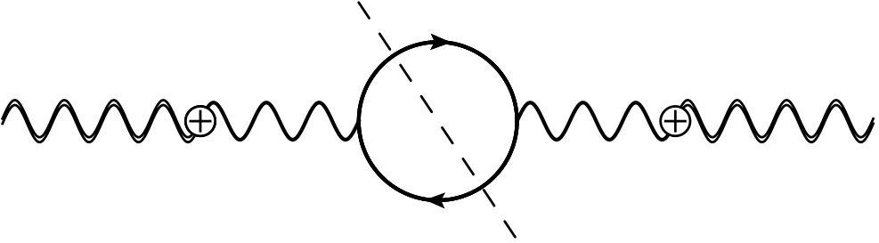
In a thermal bath, a propagating dark photon can mix with an ordinary photon, which in turn interacts with the plasma of charged particles. This process is depicted in Fig. 7. In this figure, the double (single) wiggly lines depicts the dark photon (resp. photons) propagators. The crossed circles represent their mixing and the blob is the photon polarization in the thermal bath, for instance made of relativistic particles. The dashed straight line is a cut associated to taking the imaginary part of the photon polarization tensor. In vacuum, if non-zero, this cut would be related to the decay rate of the dark photon into, say pairs, but in a plasma it includes also the dark photon creation rate from coalescence processes, i.e. Redondo:2008aa ; Weldon:1983jn . By the same token, a cut in a two-loop diagram with photon exchange within the polarization tensor would lead to the dark photon creation rate from Compton scattering, say , and pair annihilation, i.e. , etc.
On top of this, in a medium one must distinguish the behavior of the transverse and of longitudinal components of the photon polarization tensor. The latter corresponds to genuine excitations of the medium, known as plasmons, see e.g. Bellac:2011kqa . This, in turn, impacts the creation rate for production of transverse and longitudinal dark photons. As we discuss in Appendix A, in most of the range of interest for dark matter particle production in the early universe, creation of dark photons is dominantly through transverse photons An:2013yfc ; Redondo:2013lna . In a thermal bath, the latter behave essentially as massive particles, with a thermal mass (here noted ) Braaten:1993jw .
| (36) |
where is the self-energy of transverse photons and is the electric charge of the relativistic particles present in the primordial plasma. Taking this into account, the creation of transverse dark photons proceeds through an effective mixing parameter , with
| (37) |
The numerator comes from the mixing mass term in Eq. (4) and the denominator from the transverse photon propagator with virtuality . In the resonance region , one must take into account the finite width of in-medium transverse photon modes, . Production at the resonance will play an important role in the sequel, but, essentially, the substitution rule in Eq. (37) implies that the production of dark photons is suppressed at high temperature/low dark photon mass, . In particular, in the limit , , which means that there is no more connection, so that the massless dark photon case is recovered smoothly ( if , it can be rotated away and thus does not couple to SM EM currents). This phenomenon is familiar from the MSW effect in neutrino oscillations, in which oscillation into other neutrino flavors is suppressed by the frequent neutrino interactions in matter. In the opposite limit, however, , and the production of dark photon is only suppressed by the bare mixing parameter, as in vacuum.555This is all there is to if the dark photon gets its mass through the Stückelberg mechanism. The case of spontaneous symmetry breaking is discussed in Appendix B. Notice also, the substitution of Eq. (37) is for production of (transverse) dark photons on mass-shell and not in processes with exchange of virtual photons/dark photons, which are essentially insensitive to the dark photon mass. The rational behind Eq. (37) is discussed in Appendix A.
The main practical consequences of the above discussion for the production of massive dark photons and DM in the early universe is that the dark photon production is suppressed at high temperature (compared to its mass) and subsequently is resonantly enhanced once . The latter occurs at a temperature approximately equal to . This implies that if is larger than by more than one to two orders of magnitude, i.e. if , there is basically no significant production of dark photons from the SM at times that are relevant for DM production, so one recovers a mesa-shaped phase diagram similar to the massless case. Thus regimes Ib, II, IIIa and IVa are irrelevant and only regimes Ia, IIIb, IVb, Va and Vb remain, as in the massless case.
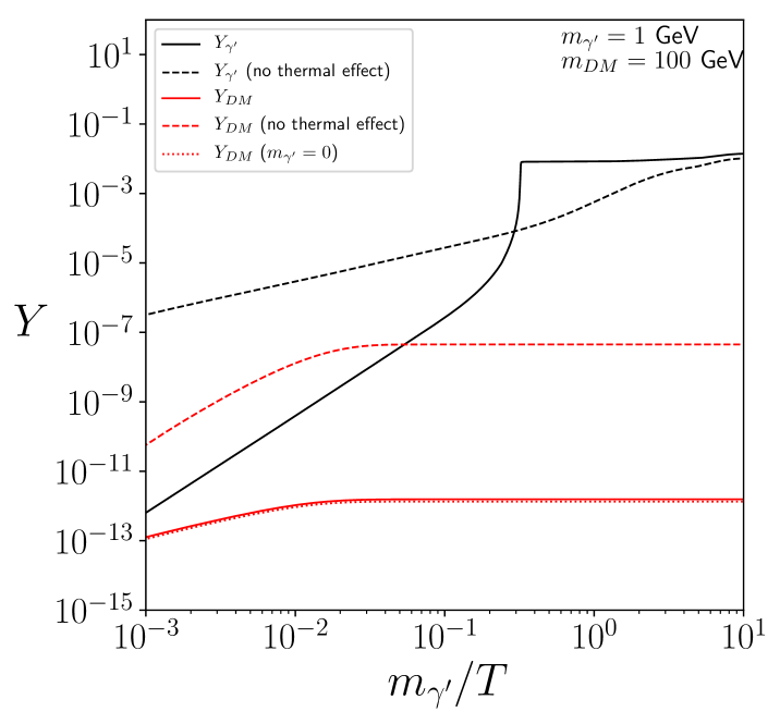
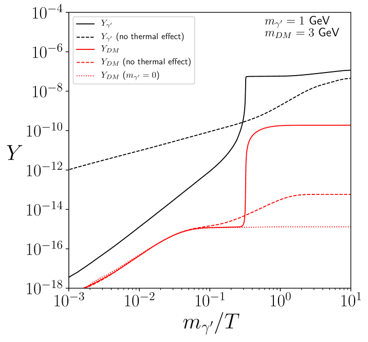
Fig. 8 gives the evolution of the dark photon and DM yields, and as a function of and for two characteristic sets of parameters. The solid (dotted) lines shows the evolution including (resp. not including) the thermal corrections to dark photon production (see Appendix A for details). The dotted lines show the evolution of taking with other parameters unchanged.
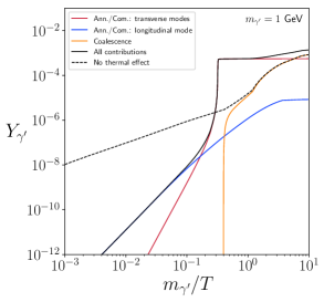
In the first panel (a) we have taken GeV, GeV and couplings that lead to the observed relic density when we include the thermal effects ( and ). Given that DM is two orders of magnitude heavier than the dark photon, this panel shows that, as expected, the production of dark photons is suppressed at high temperatures, and in particular at temperatures that are relevant for DM production, . As a result when the dark photon yield becomes important, around , the production rate of DM from dark photon pair annihilation is already too much Boltzmann suppressed to play any sizeable role in the final amount of DM (red solid line). This means that DM is mostly produced directly through driven processes and that the relic density is very close to the one obtained considering a massless dark photon (red dotted line). Thus the value of is close to the value one needs in the massless case, . If, instead, one considers the dark photon as massive but neglect the thermal corrections, there is no suppression of the dark photon production at high temperatures and DM is sizeably produced through dark photons. As a result, one obtains a larger DM relic density (red dashed line). Therefore, without thermal corrections, one would need a smaller value of . Indeed, for these masses, regime II applies so that the overall scaling of the dark photon production of DM is , in which case one would need .
The second panel (b) illustrates the opposite situation, where the dark photon and DM masses are closer, GeV, GeV. Again this is shown for values of the couplings that lead to the observed relic density taking into account thermal corrections, and . With thermal effects included, the resonance appears at a temperature close to . As the production rate of DM from dark photon is not Boltzmann suppressed when the dark photon production is resonantly enhanced, the DM abundance strongly increases, following the behavior of the dark photon abundance. Consequently, the thermal corrections strongly enhance the DM production from dark photon pair annihilation, and this both with respect to the massive case without thermal correction and with respect to the massless case. This implies that the value of needed with thermal corrections is smaller than the one required in the massless case, , and is also smaller than the one needed in the massive case without thermal corrections, . In the latter case, the production is not suppressed at high temperatures but is not boosted afterwards by any resonance in the production. See Appendix A for a more detailed study of the effect of the resonance on the DM production. Many of the features just explained can also be read off Fig. 11 which, as Fig. 6, gives the value of as a function of for GeV and GeV, but including the thermal corrections.
One related general consequence of thermal effects is that they affect the thermalization of the dark photons with the SM thermal bath. As a result, the simple criterion of Eq. (19) has to be corrected, as the production can be resonantly enhanced around (see Eq. (37) and Appendix A). Thus, taking into account thermal effects, to determine whether thermalization occurs (i.e. if reaches ) one needs to solve explicitly the Boltzmann equations. In this way, we find that the thermalization condition becomes
| (38) |
Comparing with Eq. (19), we see that, as expected, a smaller value of is needed for the dark photons to thermalize with the SM sector.
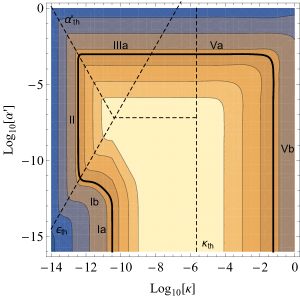
Fig. 9 gives the phase diagram obtained including the thermal effects, for the same value of and than in Fig. 4, i.e. GeV, GeV. One observes that, as expected from Fig. 8, the ”mooring bollard” shape of the phase diagram is accentuated by the thermal corrections, as the gap between the values of in the Ia and II regimes is larger. Similarly, Fig. 10 gives the phase diagram including the thermal effects for the same values of the masses as in Fig. 5.
To explain the various changes in these phase diagrams, we now revisit each regime one by one.
Freeze-in regimes: In the Ia regime, the thermal effects are small, simply because the processes are irrelevant in this regime. In regime Ib instead, the approximation we used of taking in the Boltzmann equation of Eq. (23) does not give always the correct result. Instead, one has to take the actual value of , as determined from Eq. (27). If , Eq. (27) will give and the Ib regime will disappear. Instead, if , will be enhanced by the resonance and regime Ib will be relevant for a larger range of couplings. The latter case is manifest in both phase diagrams with thermal effects. If the resonance is at ( intermediate DM masses), the freeze-in process is Boltzmann suppressed and so is not as efficient as assumed when deriving the coupling. Thus, the turn towards smaller value of can happen for larger values of , see Fig. 10 for such an example.
Sequential freeze-in: for not much smaller than , as in Figs. 9 and 10, the thermal effects lead to smaller values of than without thermal corrections (see the discussion on the second panel of Fig. 8 which gives the observed relic density along this regime). With thermal corrections, this regime leads to a vertical line in the phase diagram (as in the case without thermal corrections) because the and scalings remain unchanged. For this regime and the intermediate regime Ib merge with the standard Ia freeze-in regime, as shown in Fig. 11 for two choices of dark photon masses (solid lines). Compared to Fig. 6 (reproduced as dashed curves), the noticeable features are that resonant production of dark photon leads to even smaller values of (see the discussion revolving around Fig. 8) and that the regimes II (orange and blue curves) and Ia (green curve) merge for relatively smaller values of , for reasons explained above.
Reannihilation regimes: for not much smaller than , as for Figs. 9 and 10, we have seen above that the production of DM is boosted from the fact that the production of is resonantly boosted at a temperature which is still relevant for DM production. Thus the IIIa production regime, i.e. DM through , dominate even more over production than in the case without thermal corrections (where it was already dominant, see above). Instead, for regime IIIb, where processes dominates, applies as in the massless case.
Secluded freeze-out: for , the IVa regime, which applies in absence of thermal effects, see above, does not apply anymore as in this case the production of dark photons is highly suppressed. This is due to the fact that, at , the productions is suppressed by thermal corrections and that for there is no sizeable resonant production as the production is anyway Boltzmann suppressed. Regime IVb nevertheless can apply for , when production from the SM model is dominated by -decays, as in the massless case, see Ref. Chu:2011be . There is no IIIa to IVb transition (but only IIIa to Va transition) because, as increases, so does and thus the production of dark photons.
Freeze-out regimes: since all particles are thermalized in a single thermal bath, the effects of the above thermal corrections on the dynamics of these regimes are negligible.
V Comments on constraints
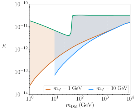
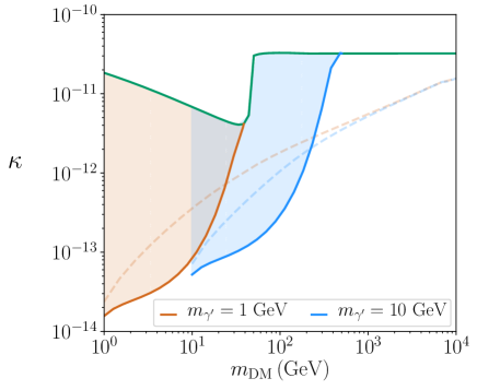
As the goal of our work is primarily the classification of the ways of producing DM, we only briefly comment on possible constraints, with a focus on the harder to test, small regimes. Indeed, as is well-known, much of the parameter space corresponding to the freeze-out and reannihilation regimes of model (1) are already constrained or excluded, including by the direct detection searches, see e.g. Chu:2011be ; Hambye:2018dpi . For the parameter ranges relevant for the freeze-in regimes, no consequent productions at colliders and indirect detection experiments of hidden sector particle is expected in general. The rates of processes relevant for those searches, or processes are typically strongly suppressed by the tiny parameters. Even so, if the mediator is light enough (meaning in the case of direct detection searches of DM in the GeV and above range), Rutherford scattering of DM on nuclei may be strongly enhanced, so that for some values of the masses direct detection experiments are already testing the freeze-in regime Hambye:2018dpi ; Chu:2011be . For lighter dark matter candidates, constraints on the parameter space of the freeze-in regime of millicharged dark matter will be possible in the future, exploiting scattering of DM off electrons, provided the dark photon is light enough, keV Essig:2011nj . Sequential freeze-in, as well as freeze-in regime Ib, in which DM is produced by the mediator, here the dark photons, extend the range of viable DM candidates toward even more feeble DM to SM couplings. In the case of the dark photon, the existence of these regimes is correlated to the mass of the dark photons, and in particular to the thermal effects discussed in Section IV. Specifically, for dark photons much lighter than DM, , the production of DM is effectively as in the massless dark photon regime, and so along the standard Ia freeze-in regime. This does not precludes the possibility that the new freeze-in regimes could also be tested by direct detection, including for other models than (1) wip .
Light dark photons and light millicharged particles are also constrained by stellar as well as CMB (cosmic microwave background) and BBN (big bang nucleosynthesis) measurements. In particular, the impact of massive, feebly coupled dark photon produced by freeze-in on cosmological observables has been studied in details Berger:2016vxi (see also Fradette:2014sza ). BBN can constrain dark photons that have an hadronic decay channel open, while CMB measurements are relevant for lighter dark photons , through their energy injection from dark photon decay into . For instance, if , as in the phase diagram of Fig. 9, then the range , which should show as an oblique band in the phase diagram of Fig. 4, is excluded by BBN, as can be seen from Fig. 5 of Ref. Berger:2016vxi . At the same time, for GeV, the sequential freeze-in runs from , roughly, so that several candidates whose abundance are set by sequential freeze-in are not excluded by BBN measurements (or, for that matter, by any other kind of currently known constraints). For GeV, the range that is constrained by BBN corresponds to and , while for and GeV, , again leaving room for viable candidates in the sequential freeze-in regime.
VI Generalization to other models
The model we considered above has a particular structure where the three connections are determined by only two independent parameters. One could therefore wonder if the overall DM production regime picture we have obtained above is deeply connected to this particular structure or is more general. In this section we would like to stress that this picture applies to other models and that in particular the sequential freeze-in regime could lead to the observed relic density in many setups. In some cases it can even be the only possible way to produce DM.
To illustrate this discussion, let us take another example, where DM is a fermionic particle , coupled to a scalar particle ,
| (39) |
From such a structure, if the scalar field does not acquire any vev, clearly one cannot create any DM particle directly from the SM (at lowest order in and ). The way to produce DM from the SM is then to create first particles and from there DM particles. Thus the three new regimes we presented above, Ib, II, IIIa and IVa are the generic possible ones, with and playing the role of and in the kinetic mixing model above, respectively. In particular if none of the interaction thermalize the sequential freeze-in is the only possible one. If instead the scalar field has a vev, it mixes with the Higgs boson and one gets a structure very similar to the one of the kinetic mixing model above, with 2 parameters inducing the 3 connections between the SM, and fluids. DM can be pair produced from SM particles through Higgs and exchange, from a combination of the and interactions (similar to the combination above), can be produced from the SM through (similar to above) and DM particles can be produced by particles through the interaction (similar to the coupling above).666Note that, unless it is forbidden in various ways, we could also have a interactions which implies a mixing too. In presence of such a term the various connections also depend on this interaction. Thus one expects a phase diagram similar to the one we obtained above.
The structure of the phase diagram of Fig. 4 is deeply connected to the fact that the sizes of the SM to mediator and mediator to DM interactions implies a lower bound on the size of the processes which connect directly SM and DM particles. For the kinetic mixing case this is quantified by the relation. For the scalar mediation example of Eq. (39) a similar phenomena occurs. If instead one would have three totally independent connections between the three sectors, still the various regimes encountered above would be possible, in particular the sequential freeze-in, but the overall picture would become more complicated, as the phase diagram becomes a 3-d diagram, rather than a 2-d one, as in Fig. 4.777A simple possibility of this kind would be to have a scalar mediator and a scalar DM particles with 3 quartic terms, . If both and have no vev, the 3 connections remain fully independent at tree level and lowest order in the couplings. Thus one has still a minimum size for one connection as a function of the other 2, but loop suppressed, which somewhat changes the overall picture. In this case one can produce dark matter in the 9 ways described above. Thus at least 9 regimes are possible, along the 5 different dynamical ways of producing DM from the SM, already mentioned above: freeze-in, sequential freeze-in, reannihilation, secluded freeze-out and freeze-out.
VII Conclusions
In this work, we have analysed the problem of DM production in the framework of a very popular model in which DM is charged under a hidden sector and interacts with SM particles through kinetic mixing. It is impressive that such a simple framework can lead to a structure of DM production regimes as rich as the one we have uncovered. Indeed, we have found that DM production out of the SM thermal bath through the kinetic mixing portal involves no less than 5 different dynamical ways, and this along 9 distinct regimes! This result, which we obtained considering the dark photon to be massive, generalizes the massless dark photon case for which 4 dynamical ways, along 5 regimes, were operative Chu:2011be . The 4 new regimes, including the one based on a new DM production mechanism which we dub “sequential freeze-in” (regime II in our classification of possible regimes), all involve prior production of dark photons by SM particles. While we focused on the kinetic mixing portal model, the structure we have found is actually characteristic of DM setups in which, on top of the SM particles and DM particles, there are other particles, akin to the dark photons, which can couple both to the SM and DM particles. More precisely, it is characteristic of models in which these 3 fluids communicate along 3 connections, which are due to 2 different interactions, here and . Such a structure thus applies to many possible DM models. Despite of the relative complexity of the DM production structure, a simple picture emerges in the phase diagram, as depicted in the plane vs . Indeed, the different production regimes follow a universal pattern composed of vertical and (almost) horizontal lines in the phase diagrams, arranged in a shape suggesting a ”mooring bollard”.
In practice, the 4 new DM production regimes turn out to be operative when the mediator, here the dark photon, is lighter than the DM particles by a factor . Below this bound, the mass of the hidden photon is effectively negligible and one recovers the regimes of DM production of the massless case studied in details in Ref. Chu:2011be . In particular, one recovers in this limit the characteristic ”mesa” shape in the phase diagrams.
The new “sequential freeze-in” dynamical production mechanism (regime II) involves the slow, out-of-equilibrium production of dark photons, followed by a slow out-of-equilibrium production of DM from these dark photons. We find interesting that such a chain of freeze-in production of particles is operative and can lead to the observed relic density even in a model as simple as the kinetic portal. The other new regimes are DM freeze-in production from a thermalized population of dark photon (Ib), reannihilation (IIIa) and secluded freeze-out (IVa) through freeze-in production of dark photons. For these new regimes, the thermal effects on dark photon production turn out to be important. On the one hand, they suppress the production of dark photons, and thus of DM, at temperature above the dark photon mass. On the other hand, they imply subsequently a resonant production of dark photon, which can strongly boost the DM production.
Acknowledgements.
This work is supported by the F.R.S.– FNRS under the Excellence of Science (EoS) project No. 30820817 – be.h “The H boson gateway to physics beyond the Standard Model”, by the FRIA , the ”Probing dark matter with neutrinos” ULB-ARC convention and the IISN convention 4.4503.15. T.H. and L.V. thank the Erwin Schrödinger International Institute for hospitality while this work was completed.Appendix A Thermal effects on dark photon production
The production rate of dark photons in a medium has been studied extensively, in particular in the sequence of articles Redondo:2008aa ; Jaeckel:2008fi ; Redondo:2008ec ; An:2013yfc ; Redondo:2013lna ; Fradette:2014sza . For comprehensiveness, we recap here the main steps of their arguments. We work in the interaction basis, treating mixing as a perturbation. Through mixing with SM photons, dark photons have a self-energy that inherits thermal features from those of photons, see Fig. 7,
| (40) |
with , where is the momentum of the virtual dark photon. In particular, its imaginary part is
| (41) |
where we set corresponding to mixing of a virtual photon into a dark photon on mass-shell. In vacuum, is related to possible photon decay channels, but in a thermal bath, has terms corresponding to both the emission and absorption rates of photons from the medium888More precisely, is to be interpreted as the rate that determines the approach to thermal equilibrium, where is the distribution function of (here) dark photons. The strange minus sign between the rates of emission and of absorption can be traced to Bose-Einstein statistics; for fermions Weldon:1983jn .
| (42) |
By detailed balance999More generally, to the fact that the amplitude squares for the emission and absorption process are equal, due to unitarity Weinberg:1979bt ., the emission rate of a photon of energy is Boltzmann suppressed compared to the corresponding absorption rate,
| (43) |
so that
| (44) |
Now, at finite temperature, on top of genuine transverse photons, the medium can also sustain the propagation of longitudinal modes or plasmon waves. These correspond to oscillations of charged particles that composed the thermal bath. Thus, in the expression of the rate of production of dark photons given by Eq. (44) one must thus distinguish transverse (T) and longitudinal (L) self-energy and so emission/absorption rates, An:2013yfc .
The transverse modes, corresponding to ordinary photons dressed by interaction with the medium, are the simplest. In the relativistic regime and to leading order in , the transverse photons simply get a thermal mass, albeit with a slight momentum dependence,
| (45) |
where is the so-called plasma frequency and the sum is over relativistic charged particles Braaten:1993jw . For later use, we mention the fact that there is no substantial wave-function renormalization for the transverse modes.
The longitudinal mode self-energy has a more involved structure. This is related to the fact that longitudinal photons do no propagate in vacuum. Still in the relativistic regime and to leading order in , the self-energy takes the form Braaten:1993jw 101010We use here the definition of the longitudinal polarization tensor of An:2013yfc ; Redondo:2013lna , , which differs from that of Braaten:1993jw , .
| (46) |
Solving for leads to
| (47) |
The behaviors of the dispersion relations of the transverse (solid blue) and longitudinal (solid orange) modes are depicted in Fig. 12.
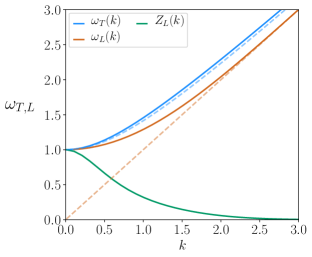
For a longitudinal plasmon mode close to on-shell, , and one can write Braaten:1993jw ; An:2013yfc ; Redondo:2013lna 111111To be clear, while we consider the real part of the self-energy only to leading order in ,the imaginary part may include higher order corrections in , so as to describe, for instance, Compton emission, etc.
| (48) |
where, using Eq. (46), the wave-function normalization is given by
| (49) |
which satisfies as but goes to zero for , as shown in Fig. 12 (green solid). This reflects the fact that the longitudinal mode mostly exists for moderate momenta. From this and (44) we get121212Expression (50) agrees with the relevant literature An:2013yfc ; Redondo:2013lna , see also Rrapaj:2019eam but perhaps a comment is in order. For instance, it may be compared with Eq. (2.7) in Redondo:2013lna using the fact that in Eq. (50) the longitudinal photon emission rates are to be calculated as in vacuum while in Ref. Redondo:2013lna (RR below) they include factors interpreted as wave-function normalization: .
| (50) |
with . This is to be compared to
| (51) |
Comparing these expressions, one sees that at large , and ,
| (52) |
As the rate for production of longitudinal photon modes itself is , due to current conservation, , the overall scaling of this ratio is . So production of dark photons is dominantly through production of longitudinal photons at high temperature, An:2013yfc ; Redondo:2013lna . At lower temperatures however, which is the regime relevant for infrared dominated freeze-in production,
| (53) |
as so production is dominantly through bona fide transverse photons An:2013yfc ; Redondo:2013lna . Thus, the production of on-shell dark photons proceeds essentially as in vacuum, but with cross-section in which the mixing parameter should be replaced by
| (54) |
legitimating the rule of thumb stated in Eq. (37).
Fig. 13 illustrates all the contributions to the production of dark photons. There, one recognises the high temperature suppression of transversal modes (Eq. 52) and the low temperature suppression of the longitudinal mode (Eq. 53).
Appendix B A note on dark Higgs production
In the body of this work, we assumed that the only relevant degrees of freedom for DM production are, beside the SM particles, the dark photon and the dark matter itself. They thus apply as such if the mass of the dark photon arises through the Stückelberg mechanism. If, instead, the is broken through the Brout-Englert-Higgs mechanism, our underlying basic assumption is that the dark Higgs () is much heavier than both the dark photon and the dark matter, i.e. that
| (55) |
where and are the dark Higgs quartic coupling and vev. We assumed, for simplicity, that the DM is vector-like so that can be taken to be independent of , a hypothesis that could be relaxed in a more elaborated scenario. Now is a (very) tiny parameter for most of the parameter space we consider, so these conditions can be easily met. If this is not the case (for instance if for some reason itself is a small parameter) then we may have e.g.
| (56) |
If this is the case, the system becomes more complex, as we must in principle take into account the abundance of particles on top of that of the DM and the dark photons, see Fig. 14.
An interesting aspect of this scenario is that the process of associated production of dark Higgs (or dark-Higgsstrahlung) is unsuppressed in the limit , and scales as Pospelov:2008jk ; Batell:2009yf
| (57) |
for large . As , the rate of production is proportional to and not as naively expected from the vertex . This result, familiar from SM Higgs physics, can be traced back to the fact that the process (57) is dominated by longitudinal emission at large energies. Hence, the connection between the SM sector and the is controlled by , precisely like the DM itself, see Fig. 14. By the same token, the connections between the , the and the DM are all driven by .
From the above discussion and the (approximate) symmetry of Fig. 14 we thus expect that the production of the dark Higgs will proceed as that of DM, starting from the freeze-in regime Ia for tiny values of , then Ib with production of and DM from in thermal equilibrium with the SM sector, etc. So the abundance of should essentially track that of DM, , and this at least as long as . Thus, if sequential freeze-in occurs, the contribution of the process should be subdominant compared to that of the process . Consequently, and while a more detailed analysis may be of interest, we tentatively conclude that, generically speaking, the presence of should not affect significantly the structure of the phase diagram depicted in Figs. 9 and 10.
As for the symmetric phase, in which , it would contain two DM candidates, as the complex scalar associated to the dark Higgs would also be stable (by charge conservation), and both would be produced at similar rates for tiny couplings. In particular, as the abundance at freeze-in is (baring production from Z boson decay, see Chu:2011be ), both particles will give (roughly) a similar contribution to the DM energy density, . While reannihilation and subsequent regimes may have a richer structure than in a scheme with a single DM candidate, we expect the phase diagram to follow essentially the ”mesa” pattern studied in Chu:2011be .
References
- (1) B. Patt and F. Wilczek, Higgs-field portal into hidden sectors, hep-ph/0605188.
- (2) X. Chu, T. Hambye and M. H. G. Tytgat, The Four Basic Ways of Creating Dark Matter Through a Portal, JCAP 1205 (2012) 034, [1112.0493].
- (3) J. Jaeckel and A. Ringwald, The Low-Energy Frontier of Particle Physics, Ann. Rev. Nucl. Part. Sci. 60 (2010) 405–437, [1002.0329].
- (4) R. Essig et al., Working Group Report: New Light Weakly Coupled Particles, in Proceedings, 2013 Community Summer Study on the Future of U.S. Particle Physics: Snowmass on the Mississippi (CSS2013): Minneapolis, MN, USA, July 29-August 6, 2013, 2013. 1311.0029.
- (5) J. Alexander et al., Dark Sectors 2016 Workshop: Community Report, 2016. 1608.08632.
- (6) R. Foot and S. Vagnozzi, Dissipative hidden sector dark matter, Phys. Rev. D91 (2015) 023512, [1409.7174].
- (7) L. Ackerman, M. R. Buckley, S. M. Carroll and M. Kamionkowski, Dark Matter and Dark Radiation, Phys. Rev. D79 (2009) 023519, [0810.5126].
- (8) J. L. Feng, H. Tu and H.-B. Yu, Thermal Relics in Hidden Sectors, JCAP 0810 (2008) 043, [0808.2318].
- (9) J. L. Feng, M. Kaplinghat, H. Tu and H.-B. Yu, Hidden Charged Dark Matter, JCAP 0907 (2009) 004, [0905.3039].
- (10) T. Hambye, On the stability of particle dark matter, PoS IDM2010 (2011) 098, [1012.4587].
- (11) B. Holdom, Two U(1)’s and Epsilon Charge Shifts, Phys. Lett. 166B (1986) 196–198.
- (12) E. C. G. Stueckelberg, Interaction energy in electrodynamics and in the field theory of nuclear forces, Helv. Phys. Acta 11 (1938) 225–244.
- (13) F. Englert and R. Brout, Broken Symmetry and the Mass of Gauge Vector Mesons, Phys. Rev. Lett. 13 (1964) 321–323.
- (14) P. W. Higgs, Broken Symmetries and the Masses of Gauge Bosons, Phys. Rev. Lett. 13 (1964) 508–509.
- (15) J. McDonald, Thermally generated gauge singlet scalars as selfinteracting dark matter, Phys. Rev. Lett. 88 (2002) 091304, [hep-ph/0106249].
- (16) L. J. Hall, K. Jedamzik, J. March-Russell and S. M. West, Freeze-In Production of FIMP Dark Matter, JHEP 03 (2010) 080, [0911.1120].
- (17) N. Bernal, M. Heikinheimo, T. Tenkanen, K. Tuominen and V. Vaskonen, The Dawn of FIMP Dark Matter: A Review of Models and Constraints, Int. J. Mod. Phys. A32 (2017) 1730023, [1706.07442].
- (18) M. Pospelov, A. Ritz and M. B. Voloshin, Secluded WIMP Dark Matter, Phys. Lett. B662 (2008) 53–61, [0711.4866].
- (19) M. Pospelov, Secluded U(1) below the weak scale, Phys. Rev. D80 (2009) 095002, [0811.1030].
- (20) R. Foot, Experimental signatures of a massive mirror photon, hep-ph/9407331.
- (21) P. Gondolo and G. Gelmini, Cosmic abundances of stable particles: Improved analysis, Nucl. Phys. B360 (1991) 145–179.
- (22) G. L. Kane, P. Kumar, B. D. Nelson and B. Zheng, Dark matter production mechanisms with a nonthermal cosmological history: A classification, Phys. Rev. D93 (2016) 063527, [1502.05406].
- (23) M. Klasen and C. E. Yaguna, Warm and cold fermionic dark matter via freeze-in, JCAP 1311 (2013) 039, [1309.2777].
- (24) J. Redondo, Helioscope Bounds on Hidden Sector Photons, JCAP 0807 (2008) 008, [0801.1527].
- (25) J. Jaeckel, J. Redondo and A. Ringwald, Signatures of a hidden cosmic microwave background, Phys. Rev. Lett. 101 (2008) 131801, [0804.4157].
- (26) J. Redondo and M. Postma, Massive hidden photons as lukewarm dark matter, JCAP 0902 (2009) 005, [0811.0326].
- (27) H. An, M. Pospelov and J. Pradler, New stellar constraints on dark photons, Phys. Lett. B725 (2013) 190–195, [1302.3884].
- (28) J. Redondo and G. Raffelt, Solar constraints on hidden photons re-visited, JCAP 1308 (2013) 034, [1305.2920].
- (29) A. Fradette, M. Pospelov, J. Pradler and A. Ritz, Cosmological Constraints on Very Dark Photons, Phys. Rev. D90 (2014) 035022, [1407.0993].
- (30) H. A. Weldon, Simple Rules for Discontinuities in Finite Temperature Field Theory, Phys. Rev. D28 (1983) 2007.
- (31) M. L. Bellac, Thermal Field Theory. Cambridge Monographs on Mathematical Physics. Cambridge University Press, 2011. 10.1017/CBO9780511721700.
- (32) E. Braaten and D. Segel, Neutrino energy loss from the plasma process at all temperatures and densities, Phys. Rev. D48 (1993) 1478–1491, [hep-ph/9302213].
- (33) T. Hambye, M. H. G. Tytgat, J. Vandecasteele and L. Vanderheyden, Dark matter direct detection is testing freeze-in, Phys. Rev. D98 (2018) 075017, [1807.05022].
- (34) R. Essig, J. Mardon and T. Volansky, Direct Detection of Sub-GeV Dark Matter, Phys. Rev. D85 (2012) 076007, [1108.5383].
- (35) T. Hambye, M. H. Tytgat, J. Vandecasteele and L. Vanderheyden, work in progress, .
- (36) J. Berger, K. Jedamzik and D. G. E. Walker, Cosmological Constraints on Decoupled Dark Photons and Dark Higgs, JCAP 1611 (2016) 032, [1605.07195].
- (37) S. Weinberg, Cosmological Production of Baryons, Phys. Rev. Lett. 42 (1979) 850–853.
- (38) E. Rrapaj, A. Sieverding and Y.-Z. Qian, Rate of dark photon emission from electron positron annihilation in massive stars, 1904.10567.
- (39) M. Pospelov, A. Ritz and M. B. Voloshin, Bosonic super-WIMPs as keV-scale dark matter, Phys. Rev. D78 (2008) 115012, [0807.3279].
- (40) B. Batell, M. Pospelov and A. Ritz, Probing a Secluded U(1) at B-factories, Phys. Rev. D79 (2009) 115008, [0903.0363].