Thermal free energy of large Nf QED in 2+1 dimensions from weak to strong coupling

Abstract

In 2+1 dimensions, QED becomes exactly solvable for all values of the fermion charge $e$ in the limit of many fermions $N_{f}\gg 1$. We present results for the free energy density at finite temperature $T$ to next-to-leading-order in large $N_{f}$. In the naive large $N_{f}$ limit, we uncover an apparently UV-divergent contribution to the vacuum energy at order ${\cal O}(\frac{e^{6}N_{f}^{3}}{\epsilon})$, which we argue to become a finite contribution of order ${\cal O}(e^{6}N_{f}^{4})$ when resumming formally higher-order $1/N_{f}$ contributions. We find the finite-temperature free energy to be well-behaved for all values of the dimensionless coupling $e^{2}N_{f}/T$, and to be bounded by the free energy of $N_{f}$ free fermions and non-interacting QED3, respectively. We invite follow-up studies from finite-temperature lattice gauge theory at large but fixed $N_{f}$ to test our results in the regime $e^{2}N_{f}/T\gg 1$.

I Introduction

The conjectured duality between strongly coupled gauge theories and classical gravity in one higher dimension has been an extremely successful tool to effectively calculate properties of large $N$ gauge theories at strong coupling and finite temperature Maldacena (1999); Gubser et al. (1998); Itzhaki et al. (1998); Policastro et al. (2001).

Unfortunately, while generally expected to be correct, there is no formal proof of the conjecture. Furthermore, only certain gauge theories have known gravity duals, and this list does not include gauge theories that are realized in nature such as QED or QCD. Finally, while gauge-gravity duality allows calculations in a regime where the coupling of the field theory is effectively infinite, the gravity dual is just as hard (or harder) to solve than the original field theory for intermediate values of the coupling, which are often physically relevant.

This provides the motivation to revisit and generalize existing tools to solve quantum field theories (and specifically gauge theories realized in nature) at finite temperature for arbitrary (weak or strong) values of the coupling. At first glance, this project seems to be dead on arrival: if techniques existed to, say, solve QCD non-perturbatively, using gauge-gravity dual results for ${\cal N}=4$ super-Yang–Mills theory as a proxy for QCD would not have been needed. Surprisingly, however, a number of large $N$ quantum field theories can be solved at finite temperature for all values of the coupling, including scalar field theories Drummond et al. (1998); Romatschke (2019a); DeWolfe and Romatschke (2019), Wess–Zumino models DeWolfe and Romatschke (2019) and Gross–Neveu models, albeit in two spatial dimensions (2+1d).

In 3+1 dimensions, divergences requiring a renormalization program spoil much of the beauty of the exact (and sometimes analytic) results found in 2+1d. This typically leads to the large $N$ 3+1-dimensional theories exhibiting a Landau pole, as is the case for scalar theories Romatschke (2019b) and four-dimensional QED Moore (2002); Ipp et al. (2003). While the theories are still useful in the effective theory sense, cut-off effects near the Landau pole imply that in 3+1 dimensions, the strong-coupling limit of these theories is ambiguous.

For this reason, we are led to consider QED in 2+1 dimensions (“QED3”) at finite temperature in the limit of many fermions $N_{f}\gg 1$, which is free of a Landau pole, and hence is unambiguously defined for any value of the coupling (cf. Refs. D’Hoker (1982); Pisarski (1984); Appelquist et al. (1988)). Because the theory does not exhibit any logarithmic divergences at leading and next-to-leading order in large $N_{f}$, in the massless fermion case QED3 is essentially a finite quantum field theory, and there are no logarithmic scale dependencies in the coupling. This implies that the free energy $f\propto T^{3}$ of QED3 scales as the third power of the temperature, with a coefficient that is only dependent on the (dimensionless) coupling $\frac{e^{2}N_{f}}{T}$.

In this work, we determine the ratio $f/T^{3}$ in QED3 non-perturbatively for all (weak to strong) values of the dimensionless coupling $\frac{e^{2}N_{f}}{T}$ to NLO at large $N_{f}$ using well-established field theory techniques. Our results thus generalize studies of QED3 at $T=0$ Pisarski (1984); Appelquist et al. (1988) to arbitrary temperature, and may be useful as a reference for lattice gauge theory studies Azcoiti and Luo (1993); Lee and Maris (2003); Hands et al. (2002); Strouthos and Kogut (2007); Raviv et al. (2014); Karthik and Narayanan (2016), dualities found for “cousins” of QED in 2+1 dimensions Son (2015); Karch and Tong (2016); Karch et al. (2017), conformal QED3 studies Kaul and Sachdev (2008); Giombi et al. (2016), as well as condensed matter systems  Franz et al. (2002).

II Setup

Let us consider QED with $N_{f}$ massless fermions defined by the Lagrangian

$${\cal L}=-\frac{1}{4}F_{\mu\nu}F^{\mu\nu}+\bar{\psi}_{a}\left(i\not{\partial}+e\not{A}\right)\psi_{a}\,,$$ (1)

where $A_{\mu}$ is the photon gauge field, $F_{\mu\nu}=\partial_{\mu}A_{\nu}-\partial_{\nu}A_{\mu}$ is the photon field strength tensor, $\psi_{a}$ with $a=1,2,\ldots,N_{f}$ are four-component spinors (both in $D=3$ and $D=4$ space-time dimensions), $e$ is the fermion charge, and $\not{A}=\gamma_{\mu}A^{\mu}$. The Lagrangian (1) is manifestly invariant under gauge transformations. QED at finite temperature $T$ may be defined as given by the Lagrangian (1) with imaginary time on a Euclidean manifold, with the time-like direction compactified on a circle with radius $\beta=T^{-1}$ (see e.g. Laine and Vuorinen (2016)). The resulting $D$-dimensional Euclidean action is given by

$$S_{E}=\int d^{D}x\left[\frac{1}{4}F_{\mu\nu}F_{\mu\nu}+\bar{\psi}_{a}\left(\not{\partial}-ie\not{A}\right)\psi_{a}\right]\,,$$ (2)

where $A_{\mu},\psi_{a}$ are the Euclidean versions of the gauge field and the fermion, respectively, and $\not{A}=\gamma_{\mu}^{E}A_{\mu}$ with $\gamma_{0}^{E}=\gamma^{0},\gamma_{1,2,3}^{E}=-i\gamma^{1,2,3}$ the Euclidean $\gamma$-matrices. Note that while the gauge field obeys periodic boundary conditions in the time-like direction, the fermions require anti-periodic boundary conditions.

Gauge invariance of $S_{E}$ implies that there are gauge configurations $A_{\mu}$ along which $S_{E}$ does not change. The existence of these “flat directions” implies that the QED partition function, defined as $Z=\int{\cal D}Ae^{-S_{E}}$, is ill-defined, because integration along the flat directions leads to divergences. In order to make sense of the theory in the non-compact formulation, it is necessary to break gauge invariance. This is customarily done using the Faddeev–Popov formalism by introducing the ghost fields $\bar{c},c$, such that for instance in the class of covariant gauges the gauge-fixed Euclidean action becomes Laine and Vuorinen (2016)

$$S_{E}=\int d^{D}x\left[\frac{1}{4}F_{\mu\nu}F_{\mu\nu}+\bar{\psi}_{a}\left(\not{\partial}-ie\not{A}\right)\psi_{a}+\frac{1}{2\xi}\left(\partial_{\mu}A_{\mu}\right)^{2}+\partial_{\mu}\bar{c}\partial_{\mu}c\right]\,,$$ (3)

where the anti-commuting ghosts fulfill periodic boundary conditions just like the bosonic gauge field. The partition function defined from the gauge-fixed action (3) is well-defined, and hence (3) will be used as the definition of QED in the following. While not gauge invariant, the action (3) is invariant under BRST transformations

$$\delta A_{\mu}=\partial_{\mu}c\zeta\,,\quad\delta\bar{c}=\frac{1}{\xi}\partial_{\mu}A_{\mu}\zeta\,,\quad\delta c=0\,,\quad\delta\bar{\psi}_{a}=-iec\bar{\psi}_{a}\zeta\,,\quad\delta\psi_{a}=iec\psi_{a}\zeta\,,$$ (4)

where $\zeta$ is an anti-commuting space-time independent parameter such that $\{\zeta,c\}=\{\zeta,\bar{c}\}=\{\zeta,\psi_{a}\}=\{\zeta,\bar{\psi}_{a}\}=0$. BRST invariance of the action (3) guarantees that many important features of gauge theories, such as Ward–Takahashi identities, are maintained even if gauge invariance has been broken.

The gauge-fixed Euclidean action (3) may be used to evaluate properties of QED at finite temperature perturbatively when expanding $e^{-S_{E}}$ in a Taylor series around vanishing coupling $e=0$. However, it is possible to resum an infinite number of contributions in this Taylor series by suitably rewriting $S_{E}=S_{0}+S_{I}$, for instance with

$$S_{0} = \int d^{D}x\left[\frac{1}{4}F_{\mu\nu}F_{\mu\nu}+\bar{\psi}_{a}\left(\not{\partial}+m\right)\psi_{a}+\frac{1}{2\xi}\left(\partial_{\mu}A_{\mu}\right)^{2}+\partial_{\mu}\bar{c}\partial_{\mu}c\right]+\frac{1}{2}\int d^{D}xd^{D}yA_{\mu}\Pi_{\mu\nu}A_{\nu}\,,$$

$$S_{I} = -ie\int d^{D}x\bar{\psi}_{a}\not{A}\psi_{a}-\frac{1}{2}\int d^{D}xd^{D}yA_{\mu}(x)\Pi_{\mu\nu}(x-y)A_{\nu}(y)\,,$$ (5)

where the same term was added and subtracted in (3). Using $S_{0}$ instead of (3) with $e=0$ as the reference action allows one to non-perturbatively resum an infinite number of Feynman diagrams (“Dyson series”). Nevertheless, it is important to maintain BRST invariance of $S_{0}$ in order to avoid introducing gauge-dependent artifacts. One finds that BRST invariance of $S_{0}$ requires $\partial_{\mu}\Pi_{\mu\nu}=0$, which is a condition that we will check a posteriori.

Photon Self-Energy

As in Refs. Romatschke (2019c, ), the quantity $\Pi_{\mu\nu}$ is fixed by calculating the full connected photon two-point function, which in the limit $N_{f}\rightarrow\infty$ becomes

$$G_{\mu\nu}(x) = \langle A_{\mu}(x)A_{\nu}(0)\rangle\,,$$

$$= G_{\mu\nu}(x)+\int_{y,z}G_{\mu\alpha}(x-y)\left(\Pi_{\alpha\beta}(y-z)-e^{2}\langle\bar{\psi}_{a}(y)\gamma_{\alpha}\psi_{a}(y)\bar{\psi}_{b}(z)\gamma_{\beta}\psi_{b}(z)\rangle\right)G_{\beta\nu}(z)\,,$$

or, taking into account the extra minus sign arising from the fermion loop,

$$\Pi_{\mu\nu}(x)=-e^{2}N_{f}{\rm Tr}\left(\Delta(x)\gamma_{\mu}\Delta(-x)\gamma_{\nu}\right)+{\cal O}(N_{f}^{0})\,,\quad\Delta(x)=\frac{1}{N_{f}}\langle\bar{\psi}_{i}(x)\psi_{i}(0)\rangle\,.$$ (7)

Note that here $G_{\mu\nu}(x),\Delta(x)$ denote fully dressed propagators, but to leading order in large $N_{f}$ we can take the fermion propagator $\Delta(x)$ to be free. It is easiest to express the $\Delta(x)$ by going to Fourier space where

$$\psi(x)=\,\hbox{$\sum$}\!\!\!\!\!\!\!\int_{\{K\}}e^{iK\cdot x}\psi(K)\,,\quad\,\hbox{$\sum$}\!\!\!\!\!\!\!\int_{\{K\}}\equiv T\sum_{\{\omega_{n}\}}\mu^{2\epsilon}\int\frac{d^{D-1}k}{(2\pi)^{D-1}}\,,$$ (8)

where $\{\omega_{n}\}=\pi T(2n+1)$ with $n\in\mathbb{Z}$ are the fermionic Matsubara frequencies, $\mu$ is the renormalization scale parameter and we use dimensional regularization with $\epsilon>0$. With these conventions, the free fermion propagator becomes

$$\Delta(x)=\,\hbox{$\sum$}\!\!\!\!\!\!\!\int_{\{K\}}\frac{e^{-iK\cdot x}\left(-i\not{K}\right)}{K^{2}}\,,$$ (9)

which leads to the photon self-energy given by

$$\Pi_{\mu\nu}(x)=-e^{2}N_{f}\,\hbox{$\sum$}\!\!\!\!\!\!\!\int_{\{K\},\{Q\}}e^{-i(K-Q)\cdot x}\frac{{\rm Tr}\left[(-i\not{K})\gamma_{\mu}(-i\not{Q})\gamma_{\nu}\right]}{K^{2}Q^{2}}\,.$$ (10)

The trace is readily evaluated using the properties of $\gamma$-matrices, finding

$${\rm Tr}\left[(-i\not{K})\gamma_{\mu}(-i\not{Q})\gamma_{\nu}\right]=4\delta_{\mu\nu}K\cdot Q-4K_{\mu}Q_{\nu}-4K_{\nu}Q_{\mu}\,.$$

In Fourier space, the photon self-energy thus becomes

$$\Pi_{\mu\nu}(P)=-4e^{2}N_{f}\,\hbox{$\sum$}\!\!\!\!\!\!\!\int_{\{K\}}\frac{\delta_{\mu\nu}\left(K^{2}-P\cdot K\right)-2K_{\mu}K_{\nu}+K_{\mu}P_{\nu}+K_{\nu}P_{\mu}}{K^{2}(K-P)^{2}}\,.$$ (11)

Let us first calculate the zero-temperature (vacuum) part of $\Pi$, which is given by

$$\Pi_{\mu\nu}^{T=0}(P)=-4e^{2}N_{f}\mu^{2\epsilon}\int\frac{d^{D}K}{(2\pi)^{D}}\int_{0}^{1}dx\frac{\delta_{\mu\nu}\left(K^{2}-P\cdot K\right)-2K_{\mu}K_{\nu}+K_{\mu}P_{\nu}+K_{\nu}P_{\mu}}{[K^{2}x+(K-P)^{2}(1-x)]^{2}}\,.$$ (12)

Shifting the integration variable $K\rightarrow K+(1-x)P$, the momentum integration is straightforward in dimensional regularization where $D=3\rightarrow 3-2\epsilon$ with $\epsilon>0$. One finds

$$\lim_{m\rightarrow 0}\Pi_{\mu\nu}^{T=0}(P)=\frac{8e^{2}N_{f}}{(4\pi)^{D/2}}\mu^{2\epsilon}\left(\delta_{\mu\nu}-\frac{P_{\mu}P_{\nu}}{P^{2}}\right)\Gamma\left(2-\frac{D}{2}\right)\frac{\Gamma^{2}\left(\frac{D}{2}\right)}{\Gamma(D)}(P^{2})^{D/2-1}\,.$$ (13)

There are no logarithmic divergences in dimensional regularization, and one can take the limit $\epsilon\rightarrow 0$, finding Pisarski (1984)

$$\Pi_{\mu\nu}^{T=0,D=3}(P)=\frac{e^{2}N_{f}}{8}\left(\delta_{\mu\nu}-\frac{P_{\mu}P_{\nu}}{P^{2}}\right)\sqrt{P^{2}}\,.$$ (14)

At finite temperature, Lorentz covariance is broken through the presence of a local matter rest frame. This implies that $\Pi_{\mu\nu}$ may be decomposed into the most general tensor structure that can be built out of $\delta_{\mu\nu},P_{\mu}$ and the rest frame vector $n_{\mu}=\left(1,{\bf 0}\right)$. The corresponding decomposition is standard in quantum field theory (cf. Ref.Kraemmer and Rebhan (2004)) and we use the complete and orthogonal tensor basis spanned by

$${\cal A}_{\mu\nu}\equiv\delta_{\mu\nu}-\frac{P_{\mu}P_{\nu}}{P^{2}}-\frac{\tilde{n}_{\mu}\tilde{n}_{\nu}}{\tilde{n}^{2}}\,,\quad{\cal B}_{\mu\nu}\equiv\frac{\tilde{n}_{\mu}\tilde{n}_{\nu}}{\tilde{n}^{2}}\,,\quad{\cal C}_{\mu\nu}\equiv\frac{P_{\mu}P_{\nu}}{P^{2}}\,,\quad{\cal D}_{\mu\nu}\equiv\tilde{n}_{\mu}P_{\nu}+\tilde{n}_{\nu}P_{\mu}\,,$$ (15)

to evaluate the structure functions for $\Pi_{\mu\nu}=\Pi_{A}{\cal A}_{\mu\nu}+\Pi_{B}{\cal B}_{\mu\nu}+\Pi_{C}{\cal C}_{\mu\nu}+\Pi_{D}{\cal D}_{\mu\nu}$. Here $\tilde{n}_{\mu}\equiv n_{\nu}\left({\cal A}_{\mu\nu}+{\cal B}_{\mu\nu}\right)$. Evaluating $P_{\mu}\Pi_{\mu\nu}$ from (11) one finds

$$P_{\mu}\Pi_{\mu\nu}(P)=-4e^{2}N_{f}\,\hbox{$\sum$}\!\!\!\!\!\!\!\int_{\{K\}}\frac{P_{\nu}K^{2}+K_{\nu}\left(P-K\right)^{2}-K^{2}K_{\nu}}{K^{2}(K-P)^{2}}=0=\Pi_{C}P_{\nu}+P^{2}\Pi_{D}\tilde{n}_{\nu}\,,$$ (16)

which implies $\Pi_{C}=\Pi_{D}=0$ and confirms that BRST invariance is satisfied for the action (II). The structure functions $\Pi_{A},\Pi_{B}$ may be found by considering the components

$$\Pi_{\mu\mu} = (D-2)\Pi_{A}(P)+\Pi_{B}(P)=-4(D-2)e^{2}N_{f}\,\hbox{$\sum$}\!\!\!\!\!\!\!\int_{\{K\}}\frac{K^{2}-P\cdot K}{K^{2}(K-P)^{2}}\,,$$ (17)

$$\Pi_{00} = \frac{|{\bf p}|^{2}}{P^{2}}\Pi_{B}(P)=-4e^{2}N_{f}\,\hbox{$\sum$}\!\!\!\!\!\!\!\int_{\{K\}}\frac{K^{2}-P\cdot K-2k_{0}^{2}+2k_{0}p_{0}}{K^{2}(K-P)^{2}}\,.$$ (18)

The corresponding thermal sums may be evaluated using standard finite-temperature field theory methods Le Bellac (1996), and the finite temperature parts are given for instance in the appendix of Ref. Carrington and Mrowczynski (2019):

$$\Pi_{\mu\mu}^{T\neq 0}=4(D-2)e^{2}N_{f}{\rm Re}\int\frac{d^{D-1}{\bf k}}{(2\pi)^{D-1}}\frac{n_{F}(|{\bf k}|)}{|{\bf k}|}\frac{2ip_{0}|{\bf k}|+2{\bf p}\cdot{\bf k}}{2ip_{0}|{\bf k}|+2{\bf p}\cdot{\bf k}-P^{2}}\,,$$

$$\Pi_{00}^{T\neq 0}=4(D-2)e^{2}N_{f}{\rm Re}\int\frac{d^{D-1}{\bf k}}{(2\pi)^{D-1}}\frac{n_{F}(|{\bf k}|)}{|{\bf k}|}\frac{ip_{0}|{\bf k}|+2{\bf k}^{2}-{\bf p}\cdot{\bf k}}{2ip_{0}|{\bf k}|+2{\bf p}\cdot{\bf k}-P^{2}}\,,$$ (19)

where ${\rm Re}f(p_{0})=\frac{1}{2}\left(f(p_{0})+f(-p_{0})\right)$. For $D=3$, the remaining angular integration may be carried out to find

$$\Pi_{\mu\mu}^{T\neq 0,D=3}=4e^{2}N_{f}{\rm Re}\int_{0}^{\infty}\frac{dk\,n_{F}(k)}{2\pi}\left(1-\frac{\sqrt{P^{2}}}{\sqrt{P^{2}-4k^{2}-4ip_{0}k}}\right)\,,$$

$$\Pi_{00}^{T\neq 0,D=3}=4e^{2}N_{f}{\rm Re}\int_{0}^{\infty}\frac{dk\,n_{F}(k)}{2\pi}\left(1-\frac{\sqrt{P^{2}-4k^{2}-4ip_{0}k}}{\sqrt{P^{2}}}\right)\,.$$ (20)

III Partition Function for QED3

The partition function for QED3 is given by

$$Z=\int{\cal D}\bar{\psi}{\cal D}\psi{\cal D}\bar{c}{\cal D}c{\cal D}Ae^{-S_{0}-S_{I}}\,,$$ (21)

with $S_{0},S_{I}$ given in Eqns. (II). To leading and next-to-leading order in large $N_{f}$, $S_{0}$ already resums all the relevant “daisy-type” diagram contributions, such that contributions from $S_{I}$ only appear at order ${\cal O}(N_{f}^{-1})$, which we neglect. Hence the free energy density for QED3 to NLO in large $N_{f}$ is given by

$$f=-\frac{T}{V}\ln Z=f_{\rm ghost}+f_{\rm fermion}+f_{\rm photon}\,,$$ (22)

with

$$f_{\rm ghost}=-\,\hbox{$\sum$}\!\!\!\!\!\!\!\int_{K}\ln K^{2}\,,\quad f_{\rm fermion}=-2N_{f}\,\hbox{$\sum$}\!\!\!\!\!\!\!\int_{\{K\}}\ln K^{2}\,,\quad f_{\rm photon}=\frac{1}{2}\,\hbox{$\sum$}\!\!\!\!\!\!\!\int_{K}\ln{\rm det}\,G^{-1}_{\mu\nu}(K)$$ (23)

where we used the fact that all the path integrals are Gaussian in momentum space. Here $G^{-1}_{\mu\nu}(K)$ is the inverse photon propagator in momentum space, which from the expression given in $S_{0}$ takes the form

$$G_{\mu\nu}^{-1} = K^{2}\delta_{\mu\nu}-K_{\mu}K_{\nu}\left(1-\frac{1}{\xi}\right)+\Pi_{\mu\nu}(K)\,,$$ (24)

$$= \left(K^{2}+\Pi_{A}(K)\right){\cal A}_{\mu\nu}+\left(K^{2}+\Pi_{B}(K)\right){\cal B}_{\mu\nu}+\frac{K^{2}}{\xi}{\cal C}_{\mu\nu}\,,$$

using the projectors given in (15). The determinant in $f_{\rm photon}$ is given by the product of the eigenvalues of $G_{\mu\nu}^{-1}$, which are the factors multiplying the orthogonal projectors above. Therefore, the ${\cal O}\left(N_{f}^{0}\right)$ contribution to the free energy is given by

$$f_{\rm ghost}+f_{\rm photon}=\frac{1}{2}\,\hbox{$\sum$}\!\!\!\!\!\!\!\int\ln\left[\frac{\left(K^{2}+\Pi_{A}\right)\left(K^{2}+\Pi_{B}\right)}{K^{2}}\right]\,,$$ (25)

where we used that $\,\hbox{$\sum$}\!\!\!\!\!\!\!\int\,\ln\xi=0$ in dimensional regularization. The photon polarization contributions $\Pi_{A,B}$ consist of a zero-temperature piece and a finite-temperature contribution given in (14), (II) above, which for $D=3$ become

$$\Pi_{A}(P) = \Pi_{V}(P)-\frac{4e^{2}N_{f}T}{|{\bf p}|^{2}}\int_{0}^{\infty}\frac{dk}{2\pi}n_{F}(kT)\left(p_{0}^{2}+\sqrt{P^{2}}{\rm Re}\frac{(ip_{0}+2kT)^{2}}{\sqrt{P^{2}-4k^{2}T^{2}-4ip_{0}kT}}\right)$$

$$\Pi_{B}(P) = \Pi_{V}(P)+4e^{2}N_{f}T\frac{P^{2}}{|{\bf p}|^{2}}\int_{0}^{\infty}\frac{dk}{2\pi}n_{F}(kT)\left(1-\frac{1}{\sqrt{P^{2}}}{\rm Re}\sqrt{P^{2}-4k^{2}T^{2}-4ip_{0}kT}\right)$$

$$\Pi_{V}(P) = \frac{e^{2}N_{f}}{8}\sqrt{P^{2}}\,,$$ (26)

and where the integration momenta have been scaled by the temperature. Particular care must be taken when evaluating the thermal contributions in the static limit $p_{0}\rightarrow 0$, finding

$$\Pi_{A}-\Pi_{V} = -\frac{e^{2}N_{f}|{\bf p}|}{\pi}\int_{0}^{1}dyn_{F}(y|{\bf p}|/2)\frac{y^{2}}{\sqrt{1-y^{2}}}\,,$$

$$\Pi_{B}-\Pi_{V} = \frac{2e^{2}N_{f}T\ln 2}{\pi}+\frac{e^{2}N_{f}}{\pi}|{\bf p}|\int_{0}^{1}dyn_{F}(y|{\bf p}|/2)\sqrt{1-y^{2}}\,.$$ (27)

One recognizes the 2+1 dimensional Debye mass

$$m_{D}^{2}\equiv\frac{2e^{2}N_{f}T\ln 2}{\pi}\,,$$ (28)

in the zero momentum limit of $\Pi_{B}-\Pi_{V}$.

The fermion contribution and the remaining ghost contribution are easy to evaluate:

$$f_{\rm ghost} = -\frac{1}{2}\,\hbox{$\sum$}\!\!\!\!\!\!\!\int_{K}\ln K^{2}=-\int\frac{d^{2}k}{(2\pi)^{2}}\ln\left(1-e^{-k/T}\right)=\frac{\zeta(3)T^{3}}{2\pi}\,,$$

$$f_{\rm fermion} = -2N_{f}\,\hbox{$\sum$}\!\!\!\!\!\!\!\int_{\{K\}}\ln K^{2}=-4N_{f}\int\frac{d^{2}k}{(2\pi)^{2}}\ln\left(1+e^{-k/T}\right)=-\frac{3N_{f}\zeta(3)T^{3}}{2\pi}\,,$$ (29)

where only the matter contribution of the thermal sums give non-vanishing contributions. For the photons, we note that

$$f_{A,B}=\frac{1}{2}\,\hbox{$\sum$}\!\!\!\!\!\!\!\int_{K}\ln\left(K^{2}+\Pi_{A,B}(K)\right)=\frac{1}{2}\,\hbox{$\sum$}\!\!\!\!\!\!\!\int_{K}\ln\left(K^{2}+\Pi_{V}(K)\right)+\frac{1}{2}\,\hbox{$\sum$}\!\!\!\!\!\!\!\int_{K}\ln\left(1+\frac{\Pi_{A,B}(K)-\Pi_{V}(K)}{K^{2}+\Pi_{V}(K)}\right)\,,$$ (30)

where for large $K$ the asymptotic form of $\Pi_{A,B}-\Pi_{V}\propto\frac{1}{K^{2}}$ means that the second term in (30) is both IR- and UV-safe, and thus can be handled numerically.

The remaining term is given by

$$f_{V} = \frac{1}{2}\,\hbox{$\sum$}\!\!\!\!\!\!\!\int_{K}\ln\left(K^{2}+\Pi_{V}(K)\right)=\frac{1}{4}\,\hbox{$\sum$}\!\!\!\!\!\!\!\int_{K}\ln K^{2}+\frac{1}{2}\,\hbox{$\sum$}\!\!\!\!\!\!\!\int_{K}\ln\left(\sqrt{K^{2}}+\frac{\Pi_{V}(K)}{\sqrt{K^{2}}}\right)\,,$$ (31)

$$= -\frac{\zeta(3)T^{3}}{4\pi}+\int\frac{d^{D}K}{(2\pi)^{D}}\left(\frac{1}{2}+n_{B}(ik_{0})\right)\ln\left(\sqrt{K^{2}}+\frac{\Pi_{V}(K)}{\sqrt{K^{2}}}\right)\,,$$

where $n_{B}(x)=\frac{1}{e^{x/T}-1}$. The thermal contribution may be rewritten by deforming the contour to run along the Minkowski axis rather than the Euclidean axis because the integrand only has a branch cut, but no singularities anywhere on the principal Riemann sheet Moore (2002). Taking the limit $\epsilon\rightarrow 0$, this leads to

$$f_{V,1}=-\int\frac{d^{2}k}{(2\pi)^{2}}\int_{k}^{\infty}\frac{d\omega}{\pi}n_{B}(\omega){\rm Im}\ln\left(\sqrt{-\omega^{2}+k^{2}}+\frac{e^{2}N_{f}}{8}\right)\,.$$ (32)

The contribution may be further simplified as

$$f_{V,1} = -\int_{0}^{\infty}\frac{d\omega}{\pi}n_{B}(\omega)\int_{0}^{\omega^{2}}\frac{d(k^{2})}{4\pi}{\rm arctan}\left(\frac{8\sqrt{\omega^{2}-k^{2}}}{e^{2}N_{f}}\right)\,,$$ (33)

$$= -\int_{0}^{\infty}\frac{d\omega}{4\pi^{2}}n_{B}(\omega)\left[\left(\frac{e^{4}N_{f}^{2}}{64}+\omega^{2}\right){\rm arctan}\frac{8\omega}{e^{2}N_{f}}-\frac{e^{2}N_{f}\omega}{8}\right]\,,$$

which is readily evaluated numerically. Alternatively, one may investigate the weak coupling ($\frac{e^{2}N_{f}}{T}\ll 1$) and strong coupling ($\frac{e^{2}N_{f}}{T}\gg 1$) limits, which are given by

$$\lim_{e^{2}N_{f}/T\rightarrow 0}f_{V,1} = -\frac{\zeta(3)T^{3}}{4\pi}+\frac{e^{2}N_{f}T^{2}}{96}+{\cal O}(e^{4}N_{f}^{2}T)\,,$$

$$\lim_{e^{2}N_{f}/T\rightarrow\infty}f_{V,1} = -\frac{4\pi^{2}T^{4}}{45e^{2}N_{f}}+{\cal O}\left(T^{5}/(e^{4}N_{f}^{2})\right)\,.$$ (34)

From this one recovers what could already have been gleaned from the original sum-integral representation in (31): for weak coupling where $\Pi_{V}\rightarrow 0$, $f_{V}=-\frac{\zeta(3)T^{3}}{2\pi}$, corresponding to the free energy density of a single bosonic degree of freedom; conversely, for strong coupling where $K^{2}+\Pi_{V}\simeq\Pi_{V}$, the $f_{V,1}$ contribution vanishes and $f_{V}=-\frac{\zeta(3)T^{3}}{4\pi}$, corresponding to $\frac{1}{2}$ degree of freedom.

III.1 Apparently divergent vacuum energy at four-loop order

Finally, let us discuss the vacuum contribution

$$f_{V,2}=\frac{1}{2}\int\frac{d^{D}K}{(2\pi)^{D}}\ln\left(\sqrt{K^{2}}+\frac{\Pi_{V}(K)}{\sqrt{K^{2}}}\right)\,,$$ (35)

which vanishes identically for both $e^{2}N_{f}=0,\infty$. However, at face value $f_{V,2}$ includes a logarithmic divergence for any finite value of $e^{2}N_{f}$. This divergence arises at four-loop order in a perturbative expansion, which can be seen by expanding (35) in powers of $\Pi_{V}\propto e^{2}N_{f}\sqrt{K^{2}}$ such that $f_{V,2}\propto(e^{2}N_{f})^{3}\int\frac{d^{D}K}{(K^{2})^{3/2}}\propto\frac{(e^{2}N_{f})^{3}}{\epsilon}$.

The appearance of the $e^{6}$ coefficient is similar to the $g^{6}$ infrared divergence encountered for non-abelian gauge theories, also known as the “Linde problem” Linde (1980). However, we believe these issues are unrelated because for the case of QED3, the apparent divergence is in the ultraviolet, not in the infrared. The naively UV divergent contribution to $f_{V,2}$ may be calculated by considering

$$g_{V,2}=\frac{1}{2}\int\frac{d^{D}K}{(2\pi)^{D}}\frac{1}{\left(K^{2}\right)^{1/2+\epsilon}+c}=\frac{c^{2}}{32\pi^{2}}\left[\frac{1}{\epsilon}+2-\gamma_{E}+\ln\frac{\mu^{2}\pi}{c^{8}}+{\cal O}(\epsilon)\right]\,,$$ (36)

in dimensional regularization where $c=\mu^{2\epsilon}\frac{8e^{2}N_{f}}{(4\pi)^{D/2}}\Gamma(2-\frac{D}{2})\frac{\Gamma^{2}(D/2)}{\Gamma(D)}$ from (13) and $\gamma_{E}$ is Euler’s constant. Subsequently integrating w.r.t. $c$ we find

$$f_{V,2}=\frac{1}{96\pi^{2}}\left(\frac{e^{2}N_{f}}{8}\right)^{3}\left[\frac{1}{\epsilon}+\frac{5}{3}+4\ln\frac{\bar{\mu}^{2}}{e^{4}N_{f}^{2}/128}+{\cal O}(\epsilon)\right]\,,$$ (37)

where $\bar{\mu}=\sqrt{4\pi e^{-\gamma_{E}}}\mu$ is the $\overline{\rm MS}$ scheme renormalization scale. The apparently divergent contribution to the free energy density at four-loop ($e^{6}$) is problematic: since there are no divergences requiring renormalization for the charge, mass or wave-function, the only way to cancel the divergence would be by adding a vacuum-energy counterterm to the Lagrangian. However, even after doing so, this would imply that the vacuum energy thus found is renormalization-scale dependent, since there are no other divergences to cancel the non-vanishing derivative $\frac{\partial f_{V}}{\partial\bar{\mu}}$. Since the free energy is a physical observable, this cannot happen.

Further inspection reveals that the problem lies with the naive $N_{f}\rightarrow\infty$ limit. It is possible to consider further corrections to the photon polarization tensor which are formally suppressed by powers of $N_{f}$, for instance at the two-loop level, cf. Ref. Grozin (2005). One two-loop contribution (which by itself is not gauge invariant) originates from a non-vanishing fermion self-energy, modifying the fermion propagator as

$$\Delta^{-1}(K)\rightarrow i\not{K}\left(1+\Sigma(K)\right)\,.$$ (38)

To leading order in large $N_{f}$, $\Sigma(K)$ may be calculated by using the resummed photon propagator to find

$$\Sigma(K)\propto\frac{1}{N_{f}}\ln\frac{e^{4}N_{f}^{2}}{K^{2}}\,,$$ (39)

which in turn suggests that similar contributions of higher order in $N_{f}$ may be non-perturbatively resummed to give Pisarski (1984)

$$1+\Sigma(K)=\left(c_{0}\times\frac{e^{2}N_{f}}{\sqrt{K^{2}}}\right)^{\frac{8}{N_{f}\pi^{2}}}\,,$$ (40)

with a calculable constant $c_{0}$. Including the self-energy correction into the evaluation for the photon polarization tensor (11) then suggests the modification

$$\Pi_{V}(K)=\frac{e^{2}N_{f}}{8}\sqrt{K^{2}}\rightarrow\left(\frac{e^{2}N_{f}}{8}\right)^{1-\frac{8}{N_{f}\pi^{2}}}\left(K^{2}\right)^{1/2+\frac{4}{N_{f}\pi^{2}}}\,,$$

$$\Pi_{A,B}-\Pi_{V}\propto\frac{e^{2}N_{f}}{8}T\rightarrow\left(\frac{e^{2}N_{f}}{8}\right)^{1-\frac{8}{N_{f}\pi^{2}}}T^{1+\frac{8}{N_{f}\pi^{2}}}\,.$$ (41)

While these modifications do not modify most of the results for the free energy discussed above at the ${\cal O}(N_{f}^{0})$ level, there are two notable exceptions.

First, consider the contribution $f_{V,2}$ in light of these non-perturbative resummations of formally sub-leading $1/N_{f}$ corrections. Expanding (35) in powers of $\Pi_{V}$ as before, but with $\Pi_{V}\propto\sqrt{K^{2}}^{1+\frac{8}{N_{f}\pi^{2}}}$ one finds that the four-loop perturbative expression is finite in dimensional regularization because $\frac{8}{N_{f}\pi^{2}}$ takes over the role of $\epsilon$. Hence we find

$$f_{V,2}\rightarrow\frac{1}{2}\int\frac{d^{D}K}{(2\pi)^{D}}\ln\left[\left(K^{2}\right)^{1/2-\frac{4}{N_{f}\pi^{2}}}+\left(\frac{e^{2}N_{f}}{8}\right)^{1-\frac{8}{N_{f}\pi^{2}}}\right]\propto\left(\frac{e^{2}N_{f}}{8}\right)^{3}\times N_{f}\,.$$ (42)

Thus the result of including the naively sub-leading terms in the $1/N_{f}$ expansion is that the apparent UV divergence of the free energy gets turned into a finite contribution to order ${\cal O}(N_{f})$. Therefore, after resummation, the vacuum free energy is no longer renormalization-scale dependent, but there is a non-vanishing and finite cosmological constant contribution at order ${\cal O}(e^{6}N_{f}^{4})$.

III.2 Suppression of in-medium tensor contributions at strong coupling

The second instance where the formally sub-leading corrections (III.1) become important is in the numerical evaluation of the in-medium contribution in Eq. (30) near zero temperature. Specifically, without taking (III.1) into account, the temperature-dependence for the polarization tensor components (III) may be scaled out by taking $P\rightarrow T\hat{P}$, $e^{2}\rightarrow T\hat{e^{2}}$. As a consequence, one would expect the in-medium contributions to $\Pi_{A,B}$ to have non-vanishing contributions to the free energy $f_{A,B}$ even in the zero temperature limit.

However, taking into account (III.1), our calculation with naive in-medium contributions can only be trusted in a regime where

$$\frac{e^{2}N_{f}}{T}\ll e^{N_{f}\pi^{2}/8}\,,$$ (43)

whereas for $\frac{e^{2}N_{f}}{T}\rightarrow\infty$, the ${\cal O}(N_{f}^{0})$ photon contribution to the free energy is given by $f_{V}$ in (31).

III.3 Numerical evaluation of thermal contribution

The thermal photon polarization tensor contribution to the free energy is handled fully numerically by directly evaluating

$$f_{A,B}^{(M)}=\frac{1}{2}\,\hbox{$\sum$}\!\!\!\!\!\!\!\int_{K}\ln\left(1+\frac{\Pi_{A,B}(K)-\Pi_{V}(K)}{K^{2}+\Pi_{V}(K)}\right)\,.$$ (44)

Specifically, this is done by performing the sum over Matsubara frequencies and using Gauss-Legendre quadrature for the remaining integral as in Refs. Romatschke (2019c, ):

$$f_{A,B}^{(M)}=\frac{T^{3}}{16}\sum_{n=-M}^{M}\sum_{i=1}^{N}W_{i}\ln\left(1+\frac{\Pi_{A,B}(\omega_{n},k_{i}T)-\Pi_{V}(\omega_{n},k_{i}T)}{\omega_{n}^{2}+\Pi_{V}(\omega_{n},k_{i}T)}\right)\,,$$ (45)

where we used $k_{i}=\sqrt{\tan\left(\frac{x_{i}\pi}{2}\right)}+0^{+}$ to compactify the infinite interval including a small regulator to avoid any IR divergences. Here $x_{i},W_{i}$ are the nodes and modified weights, respectively, defined by the roots of the Legendre polynomial of order N:

$$P_{N}(x_{i})=0\,,\quad W_{i}=\frac{1}{(1-x_{i}^{2})\left(P_{N}^{\prime}(x_{i})\right)\cos^{2}\left(\frac{x_{i}\pi}{2}\right)}\,.$$ (46)

In practice, because of the symmetries of the integrand, only nodes with $n\geq 0$, $x_{i}\geq 0$ need to be summed over. Tabulated values for $x_{i}$ can be easily generated with high precision for $N$ up to $N\simeq 2000$, but in practice $N\simeq 200$ seems sufficient to obtain percent level precision.

We note that, in practice, we find that $f_{A}\leq 0$ and $f_{B}\geq 0$ and of similar magnitude for all values of the coupling. The numerical code for obtaining $f_{A,B}^{(M)}$ and $f_{V,1}$ as well as tabulated numerical results are publicly available at Romatschke (2019d).

IV Results and Discussion

The full free energy density for QED3 in the large $N_{f}$ limit is given by

$$f_{\rm QED3}=f_{\rm fermion}+f_{\rm ghost}+f_{\rm photon}\,,$$ (47)

where $f_{\rm fermion}$ and $f_{\rm ghost}$ are given in Eq. (III). Here $f_{\rm photon}=f_{A}+f_{B}$ with

$$f_{A,B}=-\frac{\zeta(3)T^{3}}{4\pi}+f_{V,1}+f_{V,2}+f_{A,B}^{(M)}$$ (48)

where $f_{V,1},f_{V,2}$ and the matter contributions $f_{A,B}^{(M)}$ are given in Eqns. (33), (37) and (45), respectively. As pointed out in section III.1, $f_{V,2}$ is UV-divergent in the naive large $N_{f}$ limit, with the expectation that this divergence gets turned into a finite ${\cal O}(N_{f})$ contribution once higher order terms in $1/N_{f}$ are resummed. Since this resummation is beyond the scope of the present work, we focus on the difference between vacuum and finite-temperature quantities where $f_{V,2}$ drops out. In particular, we study the pressure (minus the free energy density) difference

$$\frac{P(T)-P(0)}{\frac{\zeta(3)T^{3}}{2\pi}}=3N_{f}-2f_{V,1}-f_{A}^{(M)}-f_{B}^{(M)}\,,$$ (49)

where we have normalized the pressure to the pressure of a free (non-interacting) bosonic degree of freedom. Note that the normalized pressure is $3N_{f}$ and not $4N_{f}$ because in three dimensions each fermionic degree of freedom contributes only $\frac{3}{4}$ of a bosonic degree of freedom.

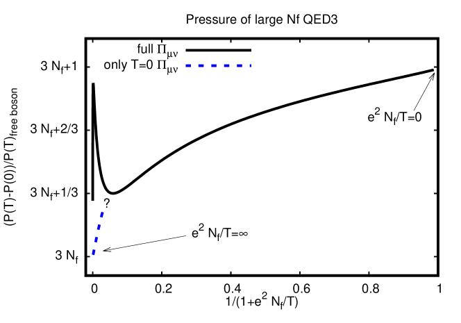
Figure 1: Normalized pressure (49) in large $N_{f}$ QED in 2+1d for all coupling values (full line). For comparison, the normalized pressure using only the vacuum polarization tensor is also shown (dashed line). Horizontal axis has been compactified in order to show the full range $\frac{e^{2}N_{f}}{T}\in[0,\infty)$. Arrows indicate weak-coupling and infinite coupling limit, respectively. The question mark indicates that we do not trust our results using the full in-medium polarization tensor to be a good approximation at large, but fixed $N_{f}$ in this region. See text for details.

As discussed above, results for $f_{V,1},f_{A}^{(M)},f_{B}^{(M)}$ can be obtained numerically for arbitrary values of $\frac{e^{2}N_{f}}{T}$. However, for reasons discussed in section III.2, for any finite $N_{f}$ we expect contributions that are naively higher order in $1/N_{f}$ to suppress the in-medium contributions to $\Pi_{A,B}$ for sufficiently low temperatures/high values of $\frac{e^{2}N_{f}}{T}$. Therefore, we expect our numerically obtained results for $f_{A,B}^{(M)}$ to lose validity at a large but finite value of $\frac{e^{2}N_{f}}{T}$. Following the arguments in Ref. Romatschke (2019e), we expect the $\frac{e^{2}N_{f}}{T}\rightarrow\infty$ limit of the pressure to be well approximated by neglecting $f_{A,B}^{(M)}$, but including $f_{V,1}$.

Our main result for the pressure is shown in Fig. 1. For weak coupling values $\frac{e^{2}N_{f}}{T}\ll 1$, we find that the normalized pressure decreases monotonically from the free theory value at $3N_{f}+1$. This trend continues up to coupling values of approximately $\frac{e^{2}N_{f}}{T}\leq 16$, at which point the normalized pressure (49) is numerically given by $3N_{f}+0.333(3)$. For $\frac{e^{2}N_{f}}{T}\geq 16$, the normalized pressure then starts to rise as a function of coupling, similar to what has been reported in the case of QED4 in Refs. Moore (2002); Ipp et al. (2003) (see Fig. 1). (Note that apparent non-monotonic behavior shown in Fig. 1 is a result of the normalization used for plotting; the (un-normalized) pressure itself is always monotonically increasing with temperature as it should.) Eventually, the normalized pressure hits a maximum below $3N_{f}+1$ and starts to decrease again for $\frac{e^{2}N_{f}}{T}\geq 100$, with the numerical evaluation of $f_{A,B}^{(M)}$ becoming more challenging in this region.

Based on the arguments given in section III.2, we suspect that for fixed, but large $N_{f}$, the normalized pressure for $\frac{e^{2}N_{f}}{T}\gg 16$ may continue to decrease towards $3N_{f}$, departing from our calculation that is using the in-medium polarization tensor evaluated in the naive large $N_{f}$ limit. This is indicated by a question mark and the result using only the vacuum polarization tensor shown in Fig. 1. We would invite follow-up studies from lattice gauge theory simulations at finite temperature in particular for $\frac{e^{2}N_{f}}{T}\geq 16$ to settle this issue.

V Acknowledgments

This work was supported by the Department of Energy, DOE award No DE-SC0017905. We would like to thank T. DeGrand, A. Hasenfratz, M. Laine, R. Pisarski, Y. Schröder, B. Svetitsky and A. Vuorinen for helpful discussions.

References

- Maldacena (1999) Juan Martin Maldacena, “The Large N limit of superconformal field theories and supergravity,” Int. J. Theor. Phys. 38, 1113–1133 (1999), [Adv. Theor. Math. Phys.2,231(1998)], arXiv:hep-th/9711200 .
- Gubser et al. (1998) Steven S. Gubser, Igor R. Klebanov, and Arkady A. Tseytlin, “Coupling constant dependence in the thermodynamics of N=4 supersymmetric Yang-Mills theory,” Nucl. Phys. B534, 202–222 (1998), arXiv:hep-th/9805156 .
- Itzhaki et al. (1998) Nissan Itzhaki, Juan Martin Maldacena, Jacob Sonnenschein, and Shimon Yankielowicz, “Supergravity and the large N limit of theories with sixteen supercharges,” Phys. Rev. D58, 046004 (1998), arXiv:hep-th/9802042 .
- Policastro et al. (2001) G. Policastro, Dan T. Son, and Andrei O. Starinets, “The Shear viscosity of strongly coupled N=4 supersymmetric Yang-Mills plasma,” Phys. Rev. Lett. 87, 081601 (2001), arXiv:hep-th/0104066 [hep-th] .
- Drummond et al. (1998) I. T. Drummond, R. R. Horgan, P. V. Landshoff, and A. Rebhan, “Foam diagram summation at finite temperature,” Nucl. Phys. B524, 579–600 (1998), arXiv:hep-ph/9708426 .
- Romatschke (2019a) Paul Romatschke, “Finite temperature CFT results for all couplings: O(N) model in 2+1 dimensions,” (2019a), arXiv:1904.09995 .
- DeWolfe and Romatschke (2019) Oliver DeWolfe and Paul Romatschke, “Strong Coupling Universality at Large N for Pure CFT Thermodynamics in 2+1 dimensions,” (2019), arXiv:1905.06355 [hep-th] .
- Romatschke (2019b) Paul Romatschke, “Analytic Transport from Weak to Strong Coupling in the O(N) model,” (2019b), arXiv:1905.09290 [hep-th] .
- Moore (2002) Guy D. Moore, “Pressure of hot QCD at large N(f),” JHEP 10, 055 (2002), arXiv:hep-ph/0209190 [hep-ph] .
- Ipp et al. (2003) Andreas Ipp, Guy D. Moore, and Anton Rebhan, “Comment on and erratum to ‘Pressure of hot QCD at large N(f)’,” JHEP 01, 037 (2003), arXiv:hep-ph/0301057 [hep-ph] .
- D’Hoker (1982) Eric D’Hoker, “PERTURBATIVE RESULTS ON QCD in three-dimensions AT FINITE TEMPERATURE,” Nucl. Phys. B201, 401–428 (1982).
- Pisarski (1984) Robert D. Pisarski, “Chiral Symmetry Breaking in Three-Dimensional Electrodynamics,” Phys. Rev. D29, 2423 (1984).
- Appelquist et al. (1988) Thomas Appelquist, Daniel Nash, and L. C. R. Wijewardhana, “Critical Behavior in (2+1)-Dimensional QED,” Phys. Rev. Lett. 60, 2575 (1988).
- Azcoiti and Luo (1993) Vicente Azcoiti and Xiang-Qian Luo, “Phase structure of compact lattice QED in three-dimensions with massless Fermions,” Mod. Phys. Lett. A8, 3635–3642 (1993), arXiv:hep-lat/9212011 [hep-lat] .
- Lee and Maris (2003) Dean Lee and Pieter Maris, “Massless QED(3) with explicit fermions,” Phys. Rev. D67, 076002 (2003), arXiv:hep-lat/0212033 [hep-lat] .
- Hands et al. (2002) S. J. Hands, J. B. Kogut, and C. G. Strouthos, “Noncompact QED(3) with N(f) greater than or equal to 2,” Nucl. Phys. B645, 321–336 (2002), arXiv:hep-lat/0208030 [hep-lat] .
- Strouthos and Kogut (2007) Costas Strouthos and John B. Kogut, “The Phases of Non-Compact QED(3),” Proceedings, 25th International Symposium on Lattice field theory (Lattice 2007): Regensburg, Germany, July 30-August 4, 2007, PoS LATTICE2007, 278 (2007), arXiv:0804.0300 [hep-lat] .
- Raviv et al. (2014) Ohad Raviv, Yigal Shamir, and Benjamin Svetitsky, “Nonperturbative beta function in three-dimensional electrodynamics,” Phys. Rev. D90, 014512 (2014), arXiv:1405.6916 [hep-lat] .
- Karthik and Narayanan (2016) Nikhil Karthik and Rajamani Narayanan, “No evidence for bilinear condensate in parity-invariant three-dimensional QED with massless fermions,” Phys. Rev. D93, 045020 (2016), arXiv:1512.02993 [hep-lat] .
- Son (2015) Dam Thanh Son, “Is the Composite Fermion a Dirac Particle?” Phys. Rev. X5, 031027 (2015), arXiv:1502.03446 [cond-mat.mes-hall] .
- Karch and Tong (2016) Andreas Karch and David Tong, “Particle-Vortex Duality from 3d Bosonization,” Phys. Rev. X6, 031043 (2016), arXiv:1606.01893 [hep-th] .
- Karch et al. (2017) Andreas Karch, Brandon Robinson, and David Tong, “More Abelian Dualities in 2+1 Dimensions,” JHEP 01, 017 (2017), arXiv:1609.04012 [hep-th] .
- Kaul and Sachdev (2008) Ribhu K. Kaul and Subir Sachdev, “Quantum criticality of U(1) gauge theories with fermionic and bosonic matter in two spatial dimensions,” Phys. Rev. B77, 155105 (2008), arXiv:0801.0723 [cond-mat.str-el] .
- Giombi et al. (2016) Simone Giombi, Grigory Tarnopolsky, and Igor R. Klebanov, “On and in Conformal QED,” JHEP 08, 156 (2016), arXiv:1602.01076 [hep-th] .
- Franz et al. (2002) M. Franz, Z Tesanovic, and O. Vafek, “QED(3) theory of pairing pseudogap in cuprates. 1. From D wave superconductor to antiferromagnet via ’algebraic’ Fermi liquid,” Phys. Rev. B66, 054535 (2002), arXiv:cond-mat/0203333 [cond-mat] .
- Laine and Vuorinen (2016) Mikko Laine and Aleksi Vuorinen, “Basics of Thermal Field Theory,” Lect. Notes Phys. 925, pp.1–281 (2016), arXiv:1701.01554 .
- Romatschke (2019c) Paul Romatschke, “Simple non-perturbative resummation schemes beyond mean-field: case study for scalar theory in 1+1 dimensions,” JHEP 03, 149 (2019c), arXiv:1901.05483 .
- (28) Paul Romatschke, “Simple non-perturbative resummation schemes beyond mean-field II: thermodynamics of scalar theory in 1+1 dimensions at arbitrary coupling,” arXiv:1903.09661 .
- Kraemmer and Rebhan (2004) Ulrike Kraemmer and Anton Rebhan, “Advances in perturbative thermal field theory,” Rept. Prog. Phys. 67, 351 (2004), arXiv:hep-ph/0310337 [hep-ph] .
- Le Bellac (1996) Michel Le Bellac, Thermal Field Theory (Cambridge University Press, 1996).
- Carrington and Mrowczynski (2019) Margaret E. Carrington and Stanislaw Mrowczynski, “Effective Coupling Constant of Plasmons,” (2019), arXiv:1907.03131 [hep-ph] .
- Linde (1980) Andrei D. Linde, “Infrared Problem in Thermodynamics of the Yang-Mills Gas,” Phys. Lett. 96B, 289–292 (1980).
- Grozin (2005) Andrey Grozin, “Lectures on QED and QCD,” in 3rd Dubna International Advanced School of Theoretical Physics Dubna, Russia, January 29-February 6, 2005 (2005) pp. 1–156, arXiv:hep-ph/0508242 [hep-ph] .
- Romatschke (2019d) P. Romatschke, “Numerical codes for QED in 2+1 dimensions,” https://github.com/paro8929/QED (2019d).
- Romatschke (2019e) Paul Romatschke, “Fractionalized Degrees of Freedom at Infinite Coupling in large Nf QED in 2+1 dimensions,” (2019e), arXiv:1908.02758 [hep-th] .