5D black holes in Einstein-Gauss-Bonnet gravity with a background of modified Chaplygin gas

Abstract

Supposing the existence of modified Chaplygin gas with the equation of state $p=A\rho-B/\rho^{\beta}$ as a cosmic background, we obtain a static spherically-symmetric black hole solution to the Einstein-Gauss-Bonnet gravitational equations in 5D spacetime. The spacetime structure of the obtained black hole solution is analyzed, also the related black hole properties are studied by calculating the thermodynamical quantities. During this process, effects of the Gauss-Bonnet coupling constant and the modified Chaplygin gas parameters on black hole solution, as well as on its thermodynamical properties are discussed. At the end, we study the quantum tunneling of scalar particles and the propagating of scalar waves within the background of modified Chaplygin gas. The study shows that the system is stable under scalar perturbations and the Hawking radiation could stop at some point, leaving an extremal black hole as remnant for evaporation.

1 Introduction

Ones of the natural modifications of general relativity (GR) in higher dimensions are the Lovelock theories where higher-curvature terms are supplemented [1]. Taking into account the first additional term of general Lovelock theory, i.e. the Gauss-Bonnet invariant, to Einstein gravity, one obtains the Einstein-Gauss-Bonnet (EGB) gravity. It’s interesting that EGB gravity can also be arisen from the low-energy limit of heterotic string theory [2, 3, 4]. It is believed that EGB gravity can avoid some of the shortcomings of Einstein gravity [5, 6, 7]. In addition, the EGB gravity consists of the Einstein-Hilbert action plus curvature-squared terms (see Refs. [8, 9, 10, 11, 12, 13] for more details), leading to field equations with no more than second derivatives of the metric, thus free of ghost [2]. Considering the EGB gravity context, black hole solutions and their thermodynamical behaviors have been investigated in much literature. The spherically symmetric black hole solutions in EGB gravity have been found in [8, 14]. The EGB black holes in anti de Sitter and de Sitter spaces have been discussed separately in [15] and [16]. Ref. [17] presented an exhaustive classification of static solutions for the five-dimensional EGB theory in vacuum. Recently, Refs. [18, 19, 20, 21, 22] concentrated on black hole solutions in 4D Gauss-Bonnet-scalar gravity with coupling between the scalar and the Gauss-Bonnet invariant.

Matter content of the Universe is still an unsolved problem in the framework of modern cosmology. The latest release of 2018 Planck full-sky maps about the CMB anisotropies [23] illustrates that baryon matter component is no more than $5\%$ for total energy density. In contrast, the invisible dark components, including dark energy and dark matter, are about $95\%$ energy density in the Universe. The dominance of the dark sector over the Universe makes the study of black holes surrounded by these mysterious field well-deserved. Quintessence is a possible candidate for dark energy, which is characterized by the linear equation of state $p_{q}=w\rho_{q}$. Significant attention has been devoted to discussion of static spherically-symmetric black hole solutions surrounded by quintessence matter and their properties [24, 25, 26, 27, 28, 29, 30, 31, 32], within which, Ref. [30] paid attention to the context of EGB gravity. Except the quintessence matter, many authors have found exact black hole solutions in EGB gravity with some other sources. Ref. [33] showed a class of dynamical black hole solutions in EGB gravity by restricting the energy-momentum tensor with some constraints. Ref. [34] derived spherically-symmetric solutions in EGB gravity with a Born-Infeld term. Ref. [35] derived electrically charged EGB black hole solutions with a nonlinear electrodynamics source given as an arbitrary power of the Maxwell invariant, and Ref. [36] obtained the topological black hole solutions in the presence of another two classes of nonlinear electrodynamics source. Ref. [37] represented EGB black holes with a background of Yang-Mills fields. Ref. [38] obtained a black hole solution of the 5D EGB theory for the string cloud model.

With regard to the Universal dark sector, there exists another possibility that the unknown energy component is a unified dark fluid which mixes dark matter and dark energy. Among the proposed unified dark fluid models, the Chaplygin gas [39] and its generalized model [40, 41] have been widely studied in order to explain the accelerating Universe [42, 43, 44]. Ref. [45] considered a model that charged static spherically-symmetric black hole is surrounded by Chaplygin-like dark fluid in the framework of Lovelock gravity. In this paper we study the static spherically-symmetric black holes surrounded by the modified Chaplygin gas (MCG) with the equation of state $p=A\rho-B/\rho^{\beta}$ in the 5-dimensional (5D) EGB gravity.

The plan of this paper is as follows. In section 2, for the MCG in 5D spacetime, we deduce its energy momentum tensor, with the help of which we obtain the static spherically-symmetric solutions to the EGB gravitational equations. Further we analyze the thermodynamical properties of the new derived black hole solution in section 3. Section 4 considers the Hawking radiation of scalar fields and discusses the scalar perturbations for the black hole solution. Section 5 gives the conclusion. For completeness, we give the EGB black hole solution and related thermodynamical quantities in D-dimensional spacetime with Appendix A.

We use units which fix the speed of light and the 5D gravitational constant via $8\pi G_{5}=c=1$, and use the metric signature ($-,\;+,\;+,\;\cdots,\;+$).

2 Surrounded black hole solutions in Einstein-Gauss-Bonnet gravity

2.1 The Einstein-Gauss-Bonnet theory

The Lovelock theory is an extension of the general relativity to higher-dimensions. In this theory the first and second order terms correspond to the Einstein-Hilbert and Gauss-Bonnet terms, respectively. The action for 5D EGB gravity with matter field reads

$$\mathcal{S}=\frac{1}{2}\int_{\mathcal{M}}d^{5}x\sqrt{-g}\left[\mathcal{L}_{E}+\alpha\mathcal{L}_{GB}\right]+\mathcal{S}_{M}.$$ (2.1)

$\mathcal{S}_{M}$ denotes the action associated with matter and $\alpha$ is coupling constant that we assume to be non-negative. The Einstein term is $\mathcal{L}_{E}=R$, and the second-order Gauss-Bonnet term $\mathcal{L}_{GB}$ is

$$\mathcal{L}_{GB}=R_{\mu\nu\gamma\delta}R^{\mu\nu\gamma\delta}-4R_{\mu\nu}R^{\mu\nu}+R^{2}.$$ (2.2)

Here, $R_{\mu\nu}$, $R_{\mu\nu\gamma\delta\text{}}$, and $R$ are the Ricci tensor, Riemann tensor, and Ricci scalar, respectively. The variation of the action with respect to the metric $g_{\mu\nu}$ gives the EGB equation:

$$G_{\mu\nu}\equiv G_{\mu\nu}^{E}+\alpha G_{\mu\nu}^{GB}=T_{\mu\nu},$$ (2.3)

where $G_{\mu\nu}^{E}$ is the Einstein tensor while $G_{\mu\nu}^{GB}$ is given explicitly by

$$G_{\mu\nu}^{GB}=-\frac{1}{2}\mathcal{L}_{GB}g_{\mu\nu}+2\left[-R_{\mu\rho\sigma\eta}{R_{\nu}}^{\rho\sigma\eta}-2R_{\mu\rho\nu\sigma}R^{\rho\sigma}-2R_{\mu\sigma}R_{\ \nu}^{\sigma}+RR_{\mu\nu}\right],$$ (2.4)

and $T_{\mu\nu}$ is the energy-momentum tensor of the matter that we consider as modified Chaplygin gas. We note that the divergence of EGB tensor $G_{\mu\nu}^{GB}$ vanishes. Here, we want to obtain 5D static spherically symmetric solutions of Eq. (2.3) in the background of the modified Chaplygin gas and investigate the related properties. We assume that the metric has the form:

$$\mathrm{d}s^{2}=-f(r)\mathrm{d}t^{2}+\frac{1}{f(r)}\mathrm{d}r^{2}+r^{2}(\mathrm{d}\theta^{2}+\mathrm{sin}^{2}\theta\mathrm{d}\phi^{2}+\mathrm{sin}^{2}\theta\mathrm{sin}^{2}\phi\mathrm{d}\varphi^{2}),$$ (2.5)

where we restrict the curvature of 3D hypersurface to $\kappa=1$. Using this metric ansatz, the EGB field equation (2.3) reduces to

$${G_{t}}^{t} = {G_{r}}^{r}=\frac{3}{2r^{2}}\left[rf^{\prime}+2(f-1)\right]-\frac{6\alpha}{r^{3}}\left[(f-1)f^{\prime}\right],$$

$${G_{\theta}}^{\theta} = {G_{\phi}}^{\phi}={G_{\varphi}}^{\varphi}=\frac{1}{2r^{2}}\left[r^{2}f^{\prime\prime}+4rf^{\prime}+2(f-1)\right]-\frac{\alpha}{r^{2}}\left[2(f-1)f^{\prime\prime}+2f^{\prime 2}\right].$$ (2.6)

2.2 Modified Chaplygin gas surrounding a black hole

We study the MCG with the equation of state (EoS) $p=A\rho-\frac{B}{\rho^{\beta}}$ [46, 47], where $A,B$ are positive parameters and $\beta$ stays in the interval $0\leq\beta\leq 1$. For 5D spherically-symmetric spacetime, the energy-momentum tensor components of the MCG should have the general expression

$${T}_{t}{}^{t}=\chi(r),~{}~{}{T}_{t}{}^{i}=0,~{}~{}{T}_{i}{}^{j}=\xi(r)\frac{r_{i}r^{j}}{r_{n}r^{n}}+\eta(r)\delta_{i}{}^{j},$$ (2.7)

where the form for energy-momentum tensor was first considered by Kiselev when studying static spherically-symmetric quintessence surrounding a black hole [24]. Since we are considering static spherically-symmetric spacetime, the $r-r$ component of the energy-momentum tensor should be equal to the $t-t$ component, i.e.,

$${{T}_{t}}^{t}={{T}_{r}}^{r}=-\rho(r),$$ (2.8)

If one takes isotropic average over the angles,

$$\langle r_{i}r^{j}\rangle=\frac{r_{n}r^{n}\delta_{i}{}^{j}}{4},$$ (2.9)

one obtains

$$\langle{T}_{i}{}^{j}\rangle=\Big{(}\frac{\xi(r)}{4}+\eta(r)\Big{)}\delta_{i}{}^{j}=p(r)\delta_{i}{}^{j}=\Big{(}A\rho(r)-\frac{B}{[\rho(r)]^{\beta}}\Big{)}\delta_{i}{}^{j}.$$ (2.10)

Considering Eqs. (2.8) and (2.10), $\xi(r)$ and $\eta(r)$ should be expressed as

$$\xi(r)=a_{1}\rho(r)+\frac{b_{1}}{[\rho(r)]^{\beta}},~{}~{}\eta(r)=a_{2}\rho(r)+\frac{b_{2}}{[\rho(r)]^{\beta}},$$ (2.11)

with the parameters $a_{i}$ and $b_{i}$, constrained by Eqs. (2.8) and (2.10), yielding:

$$a_{1}=-\frac{4}{3}(A+1),~{}~{}a_{2}=\frac{1+4A}{3},~{}~{}b_{1}=\frac{4}{3}B,~{}~{}b_{2}=-\frac{4}{3}B.$$ (2.12)

Thus the angular components of the energy-momentum tensor are obtained as

$${{T}_{\theta}}^{\theta}={{T}_{\phi}}^{\phi}={{T}_{\varphi}}^{\varphi}=\frac{1+4A}{3}\rho(r)-\frac{4B}{3[\rho(r)]^{\beta}}.$$ (2.13)

2.3 Exact solutions

Combining Eqs. (2.1), (2.8) and (2.13), one obtains the EGB gravitational equations:

$$\frac{3}{2r^{2}}\left[rf^{\prime}+2(f-1)\right]-\frac{6\alpha}{r^{3}}\left[(f-1)f^{\prime}\right]=-\rho,~{}$$

$$\frac{1}{2r^{2}}\left[r^{2}f^{\prime\prime}+4rf^{\prime}+2(f-1)\right]-\frac{\alpha}{r^{2}}\left[2(f-1)f^{\prime\prime}+2f^{\prime 2}\right]=\frac{1+4A}{3}\rho-\frac{4B}{3\rho^{\beta}}.$$ (2.14)

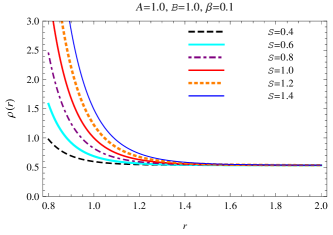
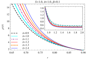
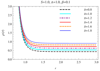
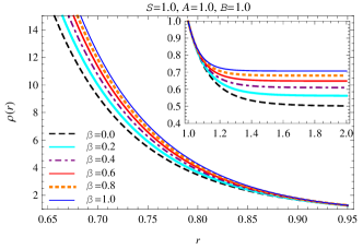
Figure 1: Energy density of the MCG as function of the radial coordinate.

Thus, we have two unknown functions $f(r)$ and $\rho(r)$ which can be determined analytically by the above two differential equations. Now, by solving the set of differential equations (2.3), one first easily obtains the solution for the energy density of MCG:

$$\rho(r)=\left(\frac{1}{1+A}\left[B+\left(\frac{S}{r^{4}}\right)^{(1+A)(1+\beta)}\right]\right)^{\frac{1}{1+\beta}},$$ (2.15)

where $S>0$ is an integration constant. We observe that $\rho(r)\rightarrow\left(\frac{B}{1+A}\right)^{\frac{1}{1+\beta}}$ when $r\rightarrow\infty$, which means that the MCG acts like a cosmological constant very far from the black hole, and it gathers more densely as it moves toward the black hole because of the gravitation, as displayed in Fig. 1. One can conclude from the figures that, the dark energy is governed by four parameters. $S$ affects $\rho(r)$ at the region near a black hole, while $B$ affects it far from the black hole. $A$ and $\beta$ can affect the energy density at regions both near and far from a black hole, however they act differently at the far region.

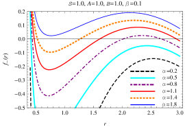
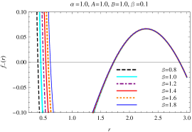
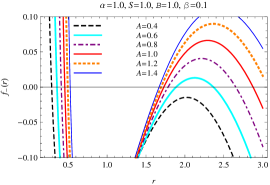
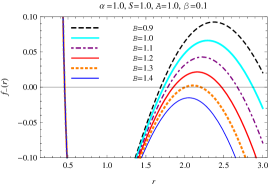
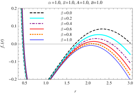
Figure 2: The $f_{-}(r)$ function in 5D Einstein-Gauss-Bonnet gravity with a background of modified Chaplygin gas for different values of $\alpha$, $S$, $A$, $B$ and $\beta$, where we set $m=2.1$.

Substituting Eq. (2.15) into the first differential equation in Eq. (2.3), we obtain two branches for the solution of $f(r)$:

$$f_{\pm}(r)=1+\frac{r^{2}}{4{\alpha}}\left(1\pm\sqrt{1+\frac{16\alpha m}{r^{4}}+\frac{4\alpha}{3}\Big{(}\frac{B}{1+A}\Big{)}^{\frac{1}{1+\beta}}\mathcal{H}}\right)$$ (2.16)

with

$$\mathcal{H} = {}_{2}F_{1}\left(\left[-\frac{1}{1+\beta},-\frac{1}{w}\right],1-\frac{1}{w},-\frac{1}{B}\left(\frac{S}{r^{4}}\right)^{w}\right),~{}$$

$$w = (1+A)(1+\beta).$$ (2.17)

We note that, $m$ is a parameter proportional to the mass of the black hole. The ADM mass $M$ of a 5D black hole relates to the mass parameter $m$ by $M=3\Sigma_{3}m$, where $\Sigma_{3}$ is the volume of the unit sphere in $\mathbb{R}^{3}$. To study the asymptotic behavior of $f_{\pm}(r)$, we take $r\rightarrow\infty$ and find that

$$f_{\pm}(r)\rightarrow 1+\frac{r^{2}}{4{\alpha}}\left(1\pm\sqrt{1+\frac{4\alpha}{3}\Big{(}\frac{B}{1+A}\Big{)}^{\frac{1}{1+\beta}}}\right),$$ (2.18)

which reveals that, given $\alpha$ with positive value, $f_{+}(r)$ tends to anti-de Sitter spacetime, while $f_{-}(r)$ tends to de Sitter spacetime. In the limit $\alpha\rightarrow 0$, the negative branch of the solution (2.16) reduces to the 5D general relativity solution. The EGB black holes surrounded by the MCG are characterized by their mass parameter $(m)$, the Gauss-Bonnet coupling constant ($\alpha$) and the four MCG parameters ($S,A,B$ and $\beta$). The effect of mass parameter $m$ on black hole solution can be referred in the next section. The $f_{-}(r)$ solution with varying values of $\alpha$, $S$, $A$, $B$ and $\beta$ is plotted in Fig. 2. We are inferred from the figures that, for appropriate parameters, the EGB black hole can have three horizons, an inner horizon, an event horizon and a cosmological horizon. It should be noted that, the radicand in Eq. (2.16) should be non-negative to keep the solution real-valued. For given mass, Gauss-Bonnet and MCG parameters, the radicand decreases to zero at the so-called branch singularity [48, 49]. Considering that the radicand at horizon radius $r_{h}$ equals to $(1+4\alpha/r_{h}^{2})^{2}$, the branch singularity should stay smaller than all the horizon radii, thus won’t obstruct our discussion on horizon radii. We can conclude from Fig. 2 that, the Gauss-Bonnet parameter $\alpha$ significantly affects the existence of black hole solution and the positions of horizon radii. The MCG parameter $S$ is liable to affect the position of inner horizon; $B$ is liable to affect the existence and position of event horizon, as well as the position of cosmological horizon; $A$ and $\beta$ both obviously affect the positions of all horizon radii, however, in different ways.

3 Thermodynamics

In this section, we discuss the thermodynamical properties of 5D MCG-surrounded black hole within Einstein-Gauss-Bonnet framework. Henceforth, we shall restrict ourselves to the negative branch of the solution (2.16). The horizon is defined as the value of $r=r_{h}$ satisfying $f_{-}(r_{h})=0$. From Eq. (2.16), the mass of the black hole is obtained in terms of the horizon radius ($r_{h}$):

$$m=\frac{r_{h}^{2}}{2}\left[1+\frac{2\alpha}{r_{h}^{2}}-\frac{r_{h}^{2}}{6}\Big{(}\frac{B}{1+A}\Big{)}^{\frac{1}{1+\beta}}\mathcal{H}(r_{h})\right],$$ (3.1)

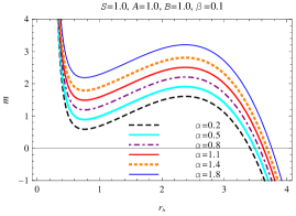
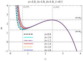
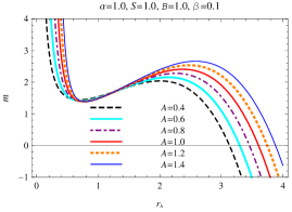
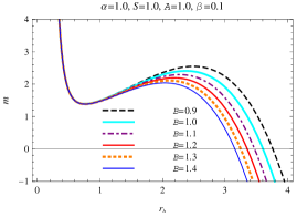
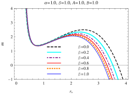
Figure 3: The mass parameter ($m$) as a function of horizon radius ($r_{h}$) in 5D Einstein-Gauss-Bonnet gravity with a background of modified Chaplygin gas for different values of $\alpha$, $S$, $A$, $B$ and $\beta$.

where $\mathcal{H}(r_{h})$ is the function value of $\mathcal{H}$ defined in Eq. (2.3) at $r=r_{h}$. The $m$ function of the black hole is plotted in Fig. 3 for various values of Gauss-Bonnet and MCG parameters. We note that, every $m-r_{h}$ curve can be divided into three parts according to the number of horizons corresponding to the same mass parameter. As an example, we discuss the $m-r_{h}$ curve for parameters $\alpha=1.0,S=0.8$, $A=1.0$, $B=1.0$ and $\beta=0.1$. The curve can be divided into $m>m_{2}$ part, $m_{2}\geq m\geq m_{1}$ part and $m_{1}>m$ part. When $m<m_{1}$ or $m>m_{2}$, the $f_{-}(r)$ solution has only a cosmological horizon (outermost horizon satisfying $f^{\prime}(r_{h})<0$); When $m_{2}>m>m_{1}$, the $f_{-}(r)$ solution has three horizons, an inner horizon (inside a event horizon and satisfying $f^{\prime}(r_{h})<0$), an event horizon ($f^{\prime}(r_{h})>0$) and a cosmological horizon. Specially, when $m=m_{1}$, the $f_{-}(r)$ solution has a degenerate event horizon ($f^{\prime}(r_{h})=0$, and $f^{\prime\prime}(r_{h})>0$) and a cosmological horizon, thus this represents a extreme solution. For $m=m_{2}$ case, the solution has an inner horizon and a degenerate horizon where event horizon coincides with cosmological horizon. The curve achieves its minimum at $r_{h}=r_{1}$, and maximum at $r_{h}=r_{2}$. In fact, within the $m_{2}>m>m_{1}$ area, the plotted $m-r_{h}$ curve represents mass-inner horizon relation at $r_{h}<r_{1}$, mass-event horizon relation at $r_{1}\leq r_{h}<r_{2}$, and mass-cosmological horizon relation at $r_{h}>r_{2}$. Fig. 3 shows an increase in the black hole mass with event horizon radius. It should be noted that the analysis above on the spacetime structure is based on the methodology proposed by Torii and Maeda in Refs. [48] and [49].

Next, we further study the Hawking temperature. The Hawking temperature associated with a black hole is defined by $T=\kappa/2\pi$ with the surface gravity $\kappa$ defined by

$$\kappa^{2}=-\frac{1}{4}g^{tt}g^{ij}g_{tt,i}\;g_{tt,j}.$$ (3.2)

Hence, the Hawking temperature for the EGB black hole surrounded by the MCG can be calculated as

$$T=\frac{r_{h}}{2\pi(r_{h}^{2}+4\alpha)}\left[1-\frac{r_{h}^{2}}{3}\rho(r_{h})\right],$$ (3.3)

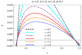
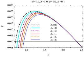
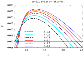
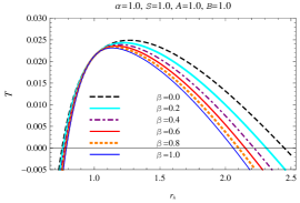
Figure 4: The Hawking temperature ($T$) as a function of horizon radius ($r_{h}$) in 5D Einstein-Gauss-Bonnet gravity with a background of modified Chaplygin gas for different values of $\alpha$, $S$, $A$, $B$ and $\beta$.

where $\rho(r_{h})$ is the function value of $\rho(r)$ defined in Eq. (2.15) at $r=r_{h}$. Note that the factor in the bracket of Eq. (3.3) modifies the pure EGB black hole temperature [51], and if we suppose the nonexistence of MCG, the pure EGB black hole temperature can be recovered as

$$T=\frac{r_{h}}{2\pi(r_{h}^{2}+4\alpha)},$$ (3.4)

and when $\alpha\rightarrow 0$, it becomes the 5D general relativity Hawking temperature which is given by $T=\frac{1}{2\pi r_{h}}$. From the curves figured in Fig. 4, one can observe that the Hawking temperature remains finite and has a peak for given Gauss-Bonnet and MCG parameters. There are two particular values of the horizon radii at which the Hawking temperature vanishes, which means that the black hole stops radiating energy here. It is interesting to note that these two horizon radii respectively correspond to the minimum and maximum points of the $m$ function. Since a physical black hole solution cannot have negative temperature, the black hole solution with an event horizon smaller than the minimum-$m$ radius or larger than the maximum-$m$ radius, is un-physical.

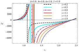
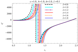
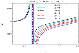
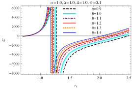
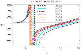
Figure 5: The specific heat ($C$) as a function of horizon radius ($r_{h}$) in 5D Einstein-Gauss-Bonnet gravity with a background of modified Chaplygin gas for different values of $\alpha$, $S$, $A$, $B$ and $\beta$.

The laws of thermodynamics can be reconciled with the existence of black hole event horizon by the so-called black hole thermodynamics, whose first law reads:

$$\mathrm{d}M=T\mathrm{d}S.$$ (3.5)

Hence, the entropy can be obtained from the integration

$$S=\int{T^{-1}\mathrm{d}M}=\int{T^{-1}\frac{\partial M}{\partial{r_{h}}}\mathrm{d}{r_{h}}}.$$ (3.6)

Now, the entropy of the EGB black hole surrounded by the MCG, reads

$$S=\frac{\Sigma_{3}r_{h}^{3}}{4\mathrm{G_{5}}}\left(1+\frac{12\alpha}{r_{h}^{2}}\right),$$ (3.7)

where $\Sigma_{3}r_{h}^{3}$ represents the horizon area of 5D black hole. Eq. (3.7) confirms the entropy obeys the area law for our case. It is interesting to note that the entropy of the black hole has no effect of the MCG parameters. This conclusion is in concordance with the string cloud background case [38] and the quintessence background case [30].

To verify the first law of thermodynamics, we next calculate the Wald entropy for the 5D black hole (2.5) with $f(r)$ given by the minus branch solution in Eq. (2.16). The Wald formulation [50] gives an expression of the entropy:

$$S_{W}=-2\pi\int_{\Sigma}\sqrt{h}\mathrm{d}V^{2}_{3}\left(\frac{\partial\mathcal{L}}{\partial R_{abcd}}\right)\varepsilon_{ab}\varepsilon_{cd},$$ (3.8)

where $\sqrt{h}\mathrm{d}V^{2}_{3}$ is the volume element on $\Sigma$ and the integral is performed on 3D space-like surface $\Sigma$. $\varepsilon_{ab}$ is the binormal vector to surface $\Sigma$ normalized as $\varepsilon_{ab}\varepsilon^{ab}=-2$, and $\mathcal{L}=\mathcal{L}_{E}+\alpha\mathcal{L}_{GB}+\mathcal{L}_{M}$ with $\mathcal{L}_{M}$ regarded as the Lagrangian for matter field. The integrand in Eq. (3.8) can be calculated as

$$\frac{\partial\mathcal{L}}{\partial R_{abcd}}\varepsilon_{ab}\varepsilon_{cd}=-2-\frac{24\alpha[1-f_{-}(r)]}{r^{2}}.$$ (3.9)

On substituting the Eq. (3.9) into the Eq. (3.8), one obtain Wald entropy of the 5D black hole (2.5) as

$$S_{W} = 2\pi\left[1+\frac{12\alpha[1-f_{-}(r_{h})]}{r_{h}^{2}}\right]\int_{\Sigma}\sqrt{h}\mathrm{d}V^{2}_{3}$$ (3.10)

$$= \frac{\Sigma_{3}r_{h}^{3}}{4\mathrm{G_{5}}}\left(1+\frac{12\alpha}{r_{h}^{2}}\right),$$

where $f_{-}(r_{h})=0$ has been used. The Wald entropy Eq. (3.10) has exactly same expression as obtained in Eq. (3.7). Since the MCG is minimally coupled to gravity, $\partial\mathcal{L}_{M}/\partial R_{abcd}=0$, leading to no effect of the MCG on the Wald entropy. The variation of Wald entropy (3.10) with respect to the horizon radius $r_{h}$ gives

$$\mathrm{d}S_{W}=\frac{3\Sigma_{3}}{4\mathrm{G_{5}}}(r_{h}^{2}+4\alpha)\mathrm{d}r_{h},$$ (3.11)

and the variation of ADM mass leads to

$$\mathrm{d}M=3\Sigma_{3}r_{h}\left(1-\frac{1}{3}r_{h}^{2}\rho(r_{h})\right)\mathrm{d}r_{h}.$$ (3.12)

Hence, with the help of Eqs. (3.3), (3.11) and (3.12), one can conclude that

$$\mathrm{d}M=T\mathrm{d}S_{W}.$$ (3.13)

Thus, we verify that the EGB black hole (2.5) characterized by the minus branch solution in Eq.(2.16), satisfies the first law of thermodynamics.

Finally, we investigate how the existence of the MCG influences the thermodynamic stability of the EGB black holes. The heat capacity of the black hole is defined as

$$C=\frac{\partial{M}}{\partial{T}}=\frac{\partial{M}}{\partial{r_{h}}}\frac{\partial{r_{h}}}{\partial{T}}.$$ (3.14)

By using Eqs. (3.1), (3.3), and (3.14), the heat capacity of the MCG-surrounded EGB black hole is calculated as

$$C=6\pi\Sigma_{3}\frac{\mathcal{X}\mathcal{Y}^{2}}{\mathcal{Z}},$$ (3.15)

where the abbreviations $\mathcal{X}$, $\mathcal{Y}$ and $\mathcal{Z}$ are given by

$$\mathcal{X}=2r_{h}-\frac{2}{3}r_{h}^{3}\rho(r_{h}),~{}~{}~{}\mathcal{Y}=r_{h}^{2}+4\alpha,~{}~{}$$

$$\mathcal{Z}=-2r_{h}^{2}+8\alpha+\frac{2}{3(1+A)}r_{h}^{2}\rho(r_{h})^{-\beta}\Big{(}r_{h}^{2}\left[-B+(4A+3)\left(\frac{S}{r^{4}}\right)^{w}\right]~{}~{}$$

$$+4\alpha\left[-3B+(4A+1)\left(\frac{S}{r^{4}}\right)^{w}\right]\Big{)},$$ (3.16)

with $w$ defined in Eq. (2.3). It is clear that the heat capacity depends on both the Gauss-Bonnet coefficient ($\alpha$), and the MCG parameters ($S$, $A$, $B$ and $\beta$). When $\alpha\rightarrow 0$, it returns to the 5D general relativity case. If in addition there is no MCG existed, it becomes

$$C=\frac{6\pi\Sigma_{3}r_{h}(r_{h}^{2}+4\alpha)^{2}}{4\alpha-r_{h}^{2}},$$ (3.17)

which is exactly same as the pure EGB case [51]. The heat capacity $C$ is plotted in Fig. 5, for different values of Gauss-Bonnet and MCG parameters. The heat capacity of a black hole hints its thermodynamical stability. The black hole is thermodynamically stable for $C>0$, while unstable for $C<0$. We note that there is a change of sign in the heat capacity around some critical horizon $r_{c}$, where $C$ is discontinuous. The critical horizon ($r_{c}$) of heat capacity coincides with the peak horizon of Hawking temperature, showing that the heat capacity diverges at horizon radius where the Hawking temperature reaches its maximum. The heat capacity vanishes at horizon radii where the mass parameter ($m$) reaches its minimum or maximum value, thus for every $C-r_{h}$ curve in Fig. 5, the $C<0$ part left to $r_{c}$ and the $C>0$ part right to $r_{c}$ are meaningless. The heat capacity is positive for $r_{h}<r_{c}$ and thereby suggesting the thermodynamical stability of a black hole. On the other hand, the black hole is unstable for $r_{h}>r_{c}$. The phase transition occurs from a higher mass black hole with the negative heat capacity to a lower mass black hole with positive heat capacity.

For the critical radius, it changes with the Gauss-Bonnet and MCG parameters, thereby affecting the thermodynamical stability. Indeed, the value of $r_{c}$ increases with the increase in $\alpha$, $S$ and $A$, while decreases with the increase in $B$ and $\beta$.

4 Tunneling and propagating of scalar fields

In this section, we first study the Hawking radiation of massive scalar particles in the 5D MCG-surrounded EGB black hole by using the semi-classical Hamilton-Jacobi method introduced in Refs. [52, 53]. Then we study the perturbative stability of the black hole solution by observing the propagating of scalar waves, following the setup introduced in Ref. [54].

4.1 Quantum tunneling of scalar particles

The movement of a scaler field $\Phi$ can be depicted by the 5D Klein-Gordon equation

$$(\partial_{a}\partial^{a}+\mu^{2})\Phi=0,$$ (4.1)

where $\mu$ denotes the mass of the scalar particle. According to the WKB approximation, $\Phi$ is of the form

$$\Phi=\mathrm{exp}\left[\frac{i}{\hbar}\sum_{i=0}^{\infty}\hbar^{i}I_{i}(t,r,\theta,\phi,\varphi)\right],$$ (4.2)

where $I_{0}$ represents the classical action of the trajectory to leading order in $\hbar$. Substituting Eq. (4.2) into Eq. (4.1) and keeping only the lowest order in $\hbar$, we obtain the Hamilton-Jacobi equation

$$\mu^{2}+f_{-}(r)(\partial_{r}I_{0})^{2}+\frac{1}{r^{2}}(\partial_{\theta}I_{0})^{2}+\frac{1}{r^{2}\mathrm{sin}^{2}{\theta}}(\partial_{\phi}I_{0})^{2}+\frac{1}{r^{2}\mathrm{sin}^{2}{\theta}\mathrm{sin}^{2}{\phi}}(\partial_{\varphi}I_{0})^{2}-\frac{1}{f_{-}(r)}(\partial_{t}I_{0})^{2}=0.$$ (4.3)

Considering the Killing vectors of the spacetime, we carry out separation of $I_{0}$

$$I_{0}=-\omega t+W(r)+\Theta(\theta,\phi,\varphi),$$ (4.4)

then Eq. (4.3) turns to

$$(\partial_{r}W)^{2}=\frac{1}{f^{2}_{-}(r)}\left[\omega^{2}-f_{-}(r)(\frac{J^{2}}{r^{2}}+\mu^{2})\right],$$ (4.5)

where $J^{2}=(\partial_{\theta}I_{0})^{2}+\frac{1}{\mathrm{sin}^{2}{\theta}}(\partial_{\phi}I_{0})^{2}+\frac{1}{\mathrm{sin}^{2}{\theta}\mathrm{sin}^{2}{\phi}}(\partial_{\varphi}I_{0})^{2}$. Thus the radial action should be calculated as

$$W_{\pm}=\pm\int\mathrm{d}r\sqrt{\frac{1}{f^{2}_{-}(r)}\left[\omega^{2}-f_{-}(r)(\frac{J^{2}}{r^{2}}+\mu^{2})\right]},$$ (4.6)

where $+(-)$ denote the outgoing (ingoing) solutions. At this point, we expand $f_{-}(r)$ around the horizon radius $r_{h}$

$$f_{-}(r)=f_{-}(r_{h})+f^{\prime}_{-}(r_{h})(r-r_{h})+\mathcal{O}((r-r_{h})^{2}),$$ (4.7)

and implement the integration along a semi-circle around the pole at $r=r_{h}$. Now, at the horizon the radial function can be given as

$$W_{\pm}=\pm i\pi\frac{\omega}{f^{\prime}_{-}(r_{h})}.$$ (4.8)

Tunneling probability for the scalar particles is given by

$$\Gamma=\mathrm{exp}\left[-\frac{4}{\hbar}ImW_{+}\right]=\mathrm{exp}\left[-\frac{\omega}{\hbar}\frac{2\pi(r^{2}_{h}+4\alpha)}{r_{h}\big{[}1-\frac{r^{2}_{h}}{3}\rho(r_{h})\big{]}}\right].$$ (4.9)

Thus the Hawking temperature of the black hole is

$$T=\frac{r_{h}}{2\pi(r_{h}^{2}+4\alpha)}\left[1-\frac{r_{h}^{2}}{3}\rho(r_{h})\right],$$ (4.10)

which is in accordance with Eq. (3.3). It can be inferred from Eq. (4.9) that, if the Hawking temperature vanishes, the particles can never tunnel from inside to outside of the event horizon. From the discussion on black hole thermodynamics in Sec. 3, it seems that a MCG-surrounded EGB black hole cannot evaporate completely and its final state could be an extremal black hole whose event horizon coincides with inner horizon. However we should be careful to make this conclusion since the perturbative stability of the black hole should be examined.

4.2 Propagating of scalar waves

We consider the case of a test scalar field $\Phi$ with mass $\mu$, also satisfying the Klein-Gordon equation in Eq. (4.1), propagating in 5D EGB spacetime with a MCG background. This field can be written by virtue of the separation of variables as follows  [55, 56, 57],

$$\Phi=R(r)Y(\theta,\phi,\varphi)\mathrm{exp}\left[-i\omega t\right].$$ (4.11)

Since the solution in the angular part is the same as in the classical case, we shall only analyze the radial part. In this case, the radial Klein-Gordon equation can be rewritten as

$$\frac{\partial_{r}\left(r^{2}f_{-}\partial_{r}R\right)}{rR}+\left(\frac{\omega^{2}}{f_{-}}-\mu^{2}\right)r^{2}=\overline{l_{3}^{2}},$$ (4.12)

where $\overline{l_{3}^{2}}=l_{3}(l_{3}+2)$ comes from the contribution of the angular equation $Y(\theta,\phi,\varphi)$ and $l_{3}\in\mathbb{Z}$ represents angular momentum quantum number. Going over to the tortoise coordinate $dr_{\ast}=dr/f(r)$, and then redefining the radial function $R_{\ast}(r_{\ast})\equiv r^{3/2}R(r)$, the last equation can be reduced to the Schr$\ddot{\mathrm{o}}$dinger wave-like form:

$$\left(\frac{\mathrm{d}}{\mathrm{d}r_{\ast}^{2}}+(\omega^{2}-V(r))\right)R_{\ast}(r_{\ast})=0,$$ (4.13)

with the effective potential $V(r)$ given by

$$V(r)=f_{-}(r)\left(\frac{\overline{l_{3}^{2}}}{r^{2}}+\frac{3f_{-}(r)}{4r^{2}}+\frac{3f_{-}^{\prime}(r)}{2r}+\mu^{2}\right).$$ (4.14)

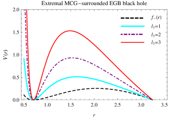
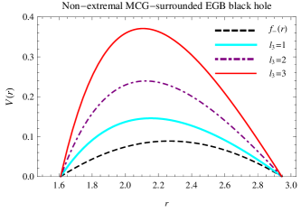
Figure 6: The effective potential ($V(r)$) of propagating scalar waves in the context of 5D Einstein-Gauss-Bonnet black hole surrounded by modified Chaplygin gas for the extremal ($m=1.33898$) and non-extremal (setting $m=2.0$) cases, with fixed values of $\alpha=1.0,S=0.8,A=1.0,B=1.0,\beta=0.1$ and $\mu=1.0$.

We plot the effective potential $V(r)$ in the background of extremal black hole and non-extremal black hole for varying values of $l_{3}$ in Fig. 6. Recalling that the positive (negative) value of the potential indicates the stability (instability) of the black hole solution, we can conclude from Fig. 6 that the MCG-surrounded EGB black hole is stable under scalar perturbations.

5 Conclusion

In this study we have obtained an exact black hole solution that integrates the surrounding modified Chaplygin gas into the framework of 5D Einstein-Gauss-Bonnet theory. A typical black hole solution has three horizons, an inner horizon, an event horizon and a cosmological horizon. Both the Gauss-Bonnet coupling constant ($\alpha$) and the modified Chaplygin gas parameters ($S,A,B,\beta$) have effects on the solution, one can find their behaviors in Fig. 2. We perform a detailed analysis of the black hole thermodynamics, focusing mainly on discussions of thermodynamical quantities like the black hole mass, Hawking temperature, entropy and specific heat. It turns out that due to correction from the modified Chaplygin gas, the thermodynamical quantities also get corrected except for the entropy which does not explicitly depend on the background matter. The entropy of a black hole in Einstein-Gauss-Bonnet gravity doesn’t obey the area law because of the non-vanishing of Gauss-Bonnet coupling constant. The black hole is thermodynamically stable with a positive heat capacity for the event horizon range $r_{h}<r_{c}$ and unstable with a negative heat capacity for $r_{h}>r_{c}$. The phase transition is characterized by the divergence of specific heat at the critical radius $r_{c}$ whose position is changing with Gauss-Bonnet coupling constant as well as with parameters of modified Chaplygin gas.

We have studied the quantum tunneling of scalar fields from the black hole by using the semi-classical method and found that the black hole radiate scalar particles with tunneling spectrum corresponding to the Hawking temperature in Eq. (3.3). The perturbative stability of black hole has also been discussed by observing the propagating of scalar waves in the concerned background. Our study shows that the black hole is stable under scalar perturbations. It seems that the Hawking radiation of the Einstein-Gauss-Bonnet black hole with surrounding modified Chaplygin gas could lead to an extremal black hole as the remanent for evaporation. The evolution of black holes within the surrounding modified Chaplygin gas is an interesting topic for future research.

Appendix A Einstein-Gauss-Bonnet black holes in D-dimensional spacetime

The energy density of the modified Chaplygin gas shows

$$\rho(r)=\left[\frac{1}{1+A}\left(B+\left[\frac{S}{r^{D-1}}\right]^{(1+A)(1+\beta)}\right)\right]^{\frac{1}{1+\beta}}.$$ (A.1)

The solution for the metric function is obtained as

$$f_{\pm}(r)=1+\frac{r^{2}}{2{\alpha}(D-3)(D-4)}\left(1\pm\sqrt{\mathcal{F}}\right)$$ (A.2)

with

$$\mathcal{F} = 1+4\alpha(D-3)(D-4)\left[\frac{2M}{(D-2)\Sigma_{D-2}r^{D-1}}+\frac{2}{(D-1)(D-2)}\Big{(}\frac{B}{1+A}\Big{)}^{\frac{1}{1+\beta}}\mathcal{H}\right],~{}$$

$$\mathcal{H} = {}_{2}F_{1}\left(\left[-\frac{1}{1+\beta},-\frac{1}{w}\right],1-\frac{1}{w},-\frac{1}{B}\left(\frac{S}{r^{D-1}}\right)^{w}\right),~{}$$

$$w = (1+A)(1+\beta),$$ (A.3)

where $\Sigma_{D-2}$ denotes the volume of the unit $(D-2)$ sphere. Again, only the minus branch solution $f_{-}(r)$ is considered as a black hole solution.

We define the horizon as $r=r_{h}$, which satisfies $f_{-}(r_{h})=0$. The mass of the black hole in terms of the black hole horizon reads

$$M=\frac{\Sigma_{D-2}}{2}\left[(D-2)r_{h}^{D-3}+(D-2)(D-3)(D-4)\alpha r_{h}^{D-5}-\frac{2r_{h}^{D-1}}{D-1}\left(\frac{B}{1+A}\right)^{\frac{1}{1+\alpha}}\mathcal{H}(r_{h})\right].$$ (A.4)

The Hawking temperature associated with black holes is calculated as

$$T=\frac{r_{h}}{4\pi\mathcal{N}(r_{h})}\left[D-3+(D-3)(D-4)(D-5)\frac{\alpha}{r_{h}^{2}}-\frac{2}{D-2}r_{h}^{2}\rho(r_{h})\right],$$ (A.5)

with

$$\mathcal{N}(r_{h})=r_{h}^{2}+2(D-3)(D-4)\alpha.$$

The entropy is given by

$$S=2\pi(D-2)\Sigma_{D-2}r_{h}^{D-4}\left[\frac{r_{h}^{2}}{D-2}+2(D-3)\alpha\right].$$ (A.6)

The heat capacity is finally calculated as

$$C=2\pi(D-2)\Sigma_{D-2}\frac{\mathcal{X}\mathcal{Y}^{2}}{\mathcal{Z}},$$ (A.7)

where

$$\mathcal{X} = (D-3)r_{h}^{D-4}+(D-3)(D-4)(D-5)\alpha r_{h}^{D-6}-\frac{2}{D-2}r_{h}^{D-2}\rho(r_{h}),$$

$$\mathcal{Y} = r_{h}^{D-3}+2(D-3)(D-4)\alpha r_{h}^{D-5},$$

$$\mathcal{Z} = \frac{2r^{2(D-4)}_{h}\rho(r_{h})}{(D-2)(1+A)}\Bigg{\{}\left[-B+\left[(D-1)A+D-2\right]\left(\frac{S}{r^{D-1}_{h}}\right)^{\omega}\right]r_{h}^{2}$$ (A.8)

$$+2(D-3)(D-4)\alpha\left[-3B+\left[(D-1)A+D-4\right]\left(\frac{S}{r^{D-1}_{h}}\right)^{\omega}\right]\Bigg{\}}$$

$$-(D-3)r_{h}^{2(D-6)}\left[r_{h}^{4}+(D-4)(D-9)\alpha r_{h}^{2}+2(D-5)(D-3)(D-4)^{2}{\alpha}^{2}\right].$$

References

- [1] D. Lovelock, The Einstein tensor and its generalizations, J. Math. Phys. 12 (1971) 498; The Four-Dimensionality of Space and the Einstein Tensor, J. Math. Phys. 13 (1972) 874.
- [2] B. Zwiebach, Curvature squared terms and string theories, Phys. Lett. B 156 (1985) 315.
- [3] D. J. Gross, E. Witten, Superstring Modifications of Einstein’s Equations, Nucl. Phys. B 277 (1986) 1.
- [4] R. R. Metsaev, A. A. Tseytlin, Two-loop -function for the generalized bosonic sigma model, Phys. Lett. B 191 (1987) 354; Curvature cubed terms in string theory effective actions, Phys. Lett. B 185 (1987) 52.
- [5] K. S. Stelle, Classical gravity with higher derivatives, Gen. Relativ. Gravit. 9 (1978) 353.
- [6] J. W. Maluf, Conformal invariance and torsion in general relativity, Gen. Relativ. Gravit. 19 (1987) 57.
- [7] M. Farhoudi, On higher order gravities, their analogy to GR, and dimensional dependent version of Duff’s trace anomaly relation, Gen. Rel. Grav. 38 (2006) 1261 [physics/0509210].
- [8] D. G. Boulware, S. Deser, String-Generated Gravity Models, Phys. Rev. Lett. 55 (1985) 2656.
- [9] B. Zumino, Gravity theories in more than four dimensions, Phys. Rept. 137 (1986) 109.
- [10] R. C. Myers, Superstring gravity and black holes, Nucl. Phys. B 289 (1987) 701.
- [11] C. G. Callan Jr., R. C. Myers, M. J. Perry, Black holes in string theory, Nucl. Phys. B 311 (1989) 673.
- [12] Y. M. Cho, I. P. Neupane and P. S. Wesson, No ghost state of Gauss-Bonnet interaction in warped background, Nucl. Phys. B 621 (2002) 388 [hep-th/0104227].
- [13] R. G. Cai, Gauss-Bonnet black holes in AdS spaces, Phys. Rev. D 65 (2002) 084014 [hep-th/0109133].
- [14] J. T. Wheeler, Symmetric Solutions to the Gauss-Bonnet Extended Einstein Equations, Nucl. Phys. B 268 (1986) 737.
- [15] Y. M. Cho, I. P. Neupane, Anti-de Sitter Black Holes, Thermal Phase Transition and Holography in Higher Curvature Gravity, Phys. Rev. D 66 (2002) 024044 [hep-th/0202140].
- [16] R. G. Cai, Q. Guo, Gauss-bonnet black holes in ds spaces, Phys. Rev. D 69 (2004) 104025 [hep-th/0311020].
- [17] G. Dotti, J. Oliva and R. Troncoso, Exact solutions for the Einstein-Gauss-Bonnet theory in five dimensions: Black holes, wormholes and spacetime horns, Phys. Rev. D 76 (2007) 064038 [hep-ph/0706.1830].
- [18] D. D. Doneva and S. S. Yazadjiev, New Gauss-Bonnet Black Holes with Curvature-Induced Scalarization in Extended Scalar-Tensor Theories, Phys. Rev. Lett. 120 (2018) 131103 [gr-qc/1711.01187].
- [19] H. O. Silva, J. Sakstein, L. Gualtieri, T. P. Sotiriou and E. Berti, Spontaneous scalarization of black holes and compact stars from a Gauss-Bonnet coupling, Phys. Rev. Lett. 120 (2018) 131104 [gr-qc/1711.02080].
- [20] J. L. Bl zquez-Salcedo, D. D. Doneva, J. Kunz and S. S. Yazadjiev,Radial perturbations of the scalarized Einstein-Gauss-Bonnet black holes, Phys. Rev. D 98 (2018) 084011 [gr-qc/1805.05755].
- [21] C. F. B. Macedo, J. Sakstein, E. Berti, L. Gualtieri, H. O. Silva and T. P. Sotiriou, Self-interactions and Spontaneous Black Hole Scalarization, Phys. Rev. D 99 (2019) 104041 [gr-qc/1903.06784].
- [22] D. D. Doneva, K. V. Staykov and S. S. Yazadjiev, Gauss-Bonnet black holes with a massive scalar field, Phys. Rev. D 99 (2019) 104045 [gr-qc/1903.08119].
- [23] N. Aghanim et al. [Planck Collaboration], Planck 2018 results. VI. Cosmological parameters, [astro-ph/1807.06209].
- [24] V. V. Kiselev, Quintessence and black holes, Class. Quant. Grav. 20 (2003) 1187 [gr-qc/0210040].
- [25] C. R. Ma, Y. X. Gui and F. J. Wang, Quintessence contribution to a Schwarzschild black hole entropy, Chin. Phys. Lett. 24 (2007) 3286.
- [26] S. Fernando, Schwarzschild black hole surrounded by quintessence: Null geodesics, Gen. Rel. Grav. 44 (2012) 1857 [gr-qc/1202.1502].
- [27] Z. Feng, L. Zhang and X. Zu, The remnants in Reissner-Nordstrm-de Sitter quintessence black hole, Mod. Phys. Lett. A 29 (2014) 1450123.
- [28] B. Malakolkalami and K. Ghaderi, Schwarzschild-anti de Sitter black hole with quintessence, Astrophys. Space Sci. 357 (2015) 112.
- [29] I. Hussain and S. Ali, Effect of quintessence on the energy of the Reissner-Nordstrm black hole, Gen. Rel. Grav. 47 (2015) 34 [gr-qc/1408.3111].
- [30] S. G. Ghosh, M. Amir and S. D. Maharaj, Quintessence background for 5D Einstein-Gauss-Bonnet black holes, Eur. Phys. J. C 77 (2017) 530 [gr-qc/1611.02936].
- [31] S. G. Ghosh, S. D. Maharaj, D. Baboolal and T. H. Lee, Lovelock black holes surrounded by quintessence, Eur. Phys. J. C 78 (2018) 90 [gr-qc/1708.03884].
- [32] J. de M.Toledo and V. B. Bezerra, Black holes with cloud of strings and quintessence in Lovelock gravity, Eur. Phys. J. C 78 (2018) 534.
- [33] A. E. Dominguez and E. Gallo, Radiating black hole solutions in Einstein-Gauss-Bonnet gravity, Phys. Rev. D 73 (2006) 064018 [gr-qc/0512150].
- [34] D. Wiltshire, Black holes in string-generated gravity models, Phys. Rev. D 38 (1988) 2445.
- [35] H. Maeda, M. Hassaine and C. Martinez, Lovelock black holes with a nonlinear Maxwell field, Phys. Rev. D 79 (2009) 044012 [gr-qc/0812.2038].
- [36] S. H. Hendi, S. Panahiyan and E. Mahmoudi, Thermodynamic analysis of topological black holes in Gauss-Bonnet gravity with nonlinear source, Eur. Phys. J. C 74 (2014) 3079 [gr-qc/1406.2357].
- [37] S. Habib Mazharimousavi and M. Halilsoy, 5D black hole solution in Einstein-Yang-Mills-Gauss-Bonnet theory, Phys. Rev. D 76 (2007) 087501 [gr-qc/0801.1562].
- [38] E. Herscovich and M. G. Richarte, Black holes in Einstein-Gauss-Bonnet gravity with a string cloud background, Phys. Lett. B 689 (2010) 192 [hep-th/1004.3754].
- [39] A. Y. Kamenshchik, U. Moschella and V. Pasquier, An Alternative to quintessence, Phys. Lett. B 511 (2001) 265 [gr-qc/0103004].
- [40] N. Bilic, G. B. Tupper and R. D. Viollier, Unification of dark matter and dark energy: The Inhomogeneous Chaplygin gas, Phys. Lett. B 535 (2002) 17 [astro-ph/0111325].
- [41] M. C. Bento, O. Bertolami and A. A. Sen, Generalized Chaplygin gas, accelerated expansion and dark energy-matter unification, Phys. Rev. D 66 (2002) 043507 [gr-qc/0202064].
- [42] D. Carturan and F. Finelli, Cosmological effects of a class of fluid dark energy models, Phys. Rev. D 68 (2003) 103501 [astro-ph/0211626].
- [43] L. Amendola, F. Finelli, C. Burigana and D. Carturan, WMAP and the generalized Chaplygin gas, JCAP 0307 (2003) 005 [astro-ph/0304325].
- [44] R. Bean and O. Dore, Are Chaplygin gases serious contenders to the dark energy throne?, Phys. Rev. D 68 (2003) 023515 [astro-ph/0301308].
- [45] X. Q. Li, B. Chen and L. l. Xing, Charged Lovelock black holes in the presence of dark fluid with a nonlinear equation of state, [gr-qc/1905.08156].
- [46] H. B. Benaoum, Accelerated universe from modified Chaplygin gas and tachyonic fluid, [hep-th/0205140].
- [47] U. Debnath, A. Banerjee and S. Chakraborty, Role of modified Chaplygin gas in accelerated universe, Class. Quant. Grav. 21 (2004) 5609 [gr-qc/0411015].
- [48] T. Torii and H. Maeda, Spacetime structure of static solutions in Gauss-Bonnet gravity: Neutral case, Phys. Rev. D 71 (2005) 124002 [hep-th/0504127].
- [49] T. Torii and H. Maeda, Spacetime structure of static solutions in Gauss-Bonnet gravity: Charged case, Phys. Rev. D 72 (2005) 064007 [hep-th/0504141].
- [50] R. M. Wald, Black hole entropy is the Noether charge, Phys. Rev. D 48 (1993) R3427.
- [51] C. Sahabandu, P. Suranyi, C. Vaz and L. C. R. Wijewardhana, Thermodynamics of static black objects in D dimensional Einstein-Gauss-Bonnet gravity with D-4 compact dimensions, Phys. Rev. D 73 (2006) 044009 [gr-qc/0509102].
- [52] M. Angheben, M. Nadalini, L. Vanzo and S. Zerbini, Hawking radiation as tunneling for extremal and rotating black holes, JHEP 0505 (2005) 014 [hep-th/0503081].
- [53] R. Kerner and R. B. Mann, Tunnelling, temperature and Taub-NUT black holes, Phys. Rev. D 73 (2006) 104010 [gr-qc/0603019].
- [54] B. Iyer, S. Iyer, C. Vishveshwara, Scalar waves in the Boulware-Deser black-hole background, Class. Quantum Grav. 6 (1989) 1627.
- [55] C. M. Harris and P. Kanti, Hawking radiation from a (4+n)-dimensional black hole: Exact results for the Schwarzschild phase, JHEP 0310 (2003) 014 [hep-ph/0309054].
- [56] V. Cardoso, M. Cavaglia and L. Gualtieri, Hawking emission of gravitons in higher dimensions: Non-rotating black holes, JHEP 0602 (2006) 021 [hep-ph/0512116].
- [57] A. S. Cornell, W. Naylor and M. Sasaki, Graviton emission from a higher-dimensional black hole, JHEP 0602 (2006) 012 [hep-ph/0510009].