5G mmWave Cooperative Positioning and Mapping using Multi-Model PHD Filter and Map Fusion

Abstract

5G millimeter wave (mmWave) signals can enable accurate positioning in vehicular networks when the base station and vehicles are equipped with large antenna arrays. However, radio-based positioning suffers from multipath signals generated by different types of objects in the physical environment. Multipath can be turned into a benefit, by building up a radio map (comprising the number of objects, object type, and object state) and using this map to exploit all available signal paths for positioning. We propose a new method for cooperative vehicle positioning and mapping of the radio environment, comprising a multiple-model probability hypothesis density filter and a map fusion routine, which is able to consider different types of objects and different fields of views. Simulation results demonstrate the performance of the proposed method.

I Introduction

5G millimeter wave (mmWave) considers the potential of large bandwidths and large antenna arrays at the user and base station (BS), which enable accurate ranging, and angle of arrival (AOA) and angle of departure (AOD) estimation [1]. Thus, 5G mmWave positioning is expected to be the next-generation cellular positioning framework [2]. Thanks to the aforementioned advantages of 5G mmWave, measurements of multipath components can be related to objects in the physical environment [3, 2, 4]. Therefore, it is possible to build up a map, which, e.g., can be reused by other users to cooperatively improve their position estimates. Such maps can also remove the need for a priori synchronization of the users, and support single BS localization [5]. Mapping and positioning using 5G can be categorized as a simultaneous localization and mapping (SLAM) problem (for SLAM basics see, e.g., [6, 7]). In addition, 5G communication links can be used to share measurements, map, or location information, leading to cooperative positioning and mapping. In 5G mmWave cooperative positioning and mapping (i.e., positioning and mapping based on measurements from 5G mmWave communication signals), there are three main tasks: (i) Vehicle positioning: determine the states (position, velocity, heading, clock bias) of the vehicles; (ii) Environment mapping: estimate the number of objects, as well as each object’s type and position; and (iii) Cooperation: fusing the collected the map information from the vehicles, and relay it to each vehicle. Even with the advantages of 5G mmWave, there are several challenges. First of all, due to the imperfect detection process at the receiver, there is a chance that objects that are inside the field-of-view (FoV) of vehicles are undetected. Secondly, the measurements may include false detections because of clutter, channel estimation error, and objects that are only visible in a short time. Third, since there are no origin-related tags on measurements, the data association must be be addressed, in either in an explicit or an implicit manner.

To solve these general challenges of SLAM, a variety of approaches have been developed. They can be coarsely divided into three classes of methods (elaborated further in Section II): geometry-based [8, 9, 10, 11], based on message passing [12, 5, 13], and based on random finite sets (RFSs) [14, 15, 16, 17, 18, 19, 20]. Among RFS-based methods for tracking and mapping, probability hypothesis density (PHD) filters [14] are widely used because they are computationally efficient alternatives that avoids explicit enumeration of the different data associations. Finally, in the considered SLAM problem, there are different types of measurements that are received by the vehicle, specifically measurements from the BS, scattering points, and reflecting surfaces [5, 13]. These different types of measurements should be handled in the mapping using a multiple model approach, with one model for each measurement type. In addition, each vehicle has a limited FoV, and has thus only observed the parts of the map space that has been inside the FoV. It follows that the multi-object densities only contain information for a subset of the map space, specifically the parts that have been inside the FoVs. For this reason, a direct application of the standard fusion [21, 22, 23] is not possible.

In this paper, we address the aforementioned challenges and propose a new method for 5G mmWave cooperative positioning and mapping that is based on RFS theory. The proposed method comprises a Rao-Blackwellized (RB) representation of the joint vehicle-map density, with particle filters for the vehicle location and a multiple-model PHD filter for the map (i.e., PHD-SLAM), similar to [24]. To update the particle weight, we theoretically derive a form of the set likelihood calculation. The PHD-SLAM filter is implemented by the Rao-Blackwellized particle filter (RBPF). Cooperation is handled using asynchronous map fusion through a modified arithmetic average (AA) approach, taking into account the different FoVs of the vehicles by designing fusion weights for AA map fusion by first decomposing the map space into mutually disjoint subsets, and then selecting weights for each subset. The BS performs map fusion with one vehicle at a time, so that through multiple interactions, each vehicle contributes to, and has access to, the global BS map. The main contributions of the paper are summarized as follows:

• For the propagation environment with multiple objects, multiple object types, and multipath measurements, we present and evaluate a novel solution to the cooperative positioning and mapping problem, based on a RB representation of the joint position-map density and a multiple-model PHD representation of the map, as well as a novel AA fusion rule.

• We derive a multiple-model PHD, which considers different measurements models, rather than different mobility models, generally considered in the literature.

• A new and theoretically sound method to update the vehicle state is provided, by deriving the closed form of the RFS-likelihood.

• By decomposing the overall source features into three mutually disjoint subsets, the fusion of each subset can be carried out independently. With this decomposition, we are able to flexibly design fusion weights for the different subsets and deal with non-overlapping sensor FoV.

• Through a Gaussian mixture implementation with online source code, the efficacy of the proposed filter and fusion approach is demonstrated in a two-vehicle scenario with 5G mmWave communication links, where all propagation paths are exploited and vehicles cooperatively map the environment, which is shown to speed up the mapping process.

The rest of the paper is organized as follows. In Section II, we discuss related works, and how our work compares to previous work. Section III describes the considered vehicular networks with 5G mmWave communication links and a problem formulation. Section IV introduces the multiple-model PHD-SLAM at the vehicle. In Section V, asynchronous map fusion is presented. Numerical results and discussions are reported in Section VI. Finally, Section VII concludes the paper.

Notation

Throughout this paper, we will use the following basic notations. Scalars are denoted by italic, e.g., $x$. Vectors are indicated by the bold lower-case letters, e.g., $\mathbf{x}$, and matrices are denoted by the bold upper-case letters, e.g., $\mathbf{X}$. Transpose of both vector and matrix is represented by superscript T, e.g., $\mathbf{x}^{\mathrm{T}}$ and $\mathbf{X}^{\mathrm{T}}$. Random sets are denoted by calligraphic, e.g., $\mathcal{X}$. We denote probability density functions (pdfs) and probability mass functions (pmfs) by $f(\cdot)$ and $p(\cdot)$, respectively. We will use the following indexing: vehicle $n$, time step $k$, particle $i$, source type $m$, Gaussian mixture component $j$.

II Related Works

In this section, we introduce the previous works for handling the aforementioned challenges in SLAM, multiple-model object tracking, and map fusion, considering methods based on geometry, methods based on message passing, and methods based on RFS theory.

In the geometry-based SLAM methods, [8] formulates the SLAM problem using the geometric relation between observations, and a non-Bayesian estimator for the user location and extended Kalman filter for mapping are introduced. MmWave imaging for one single reflected path is utilized in [9]. Neither [8] nor [9] considered the unknown number of objects or the data association uncertainty; in our paper we handle both an unknown number of objects and unknown data association. The authors in [10, 11] develop SLAM methods that are applicable when the BS location is unknown. Their solutions require four anchors to localize a node regardless of whether the four anchors are physical BSs or VAs. Therefore, at least one physical anchor is required with its corresponding VA mirrored through reflective surfaces for SLAM and obstacle detection.

In the second category, a message passing-based estimator for position and orientation of the vehicle, as well as mapping objects is introduced in [12]. In [5], the clock bias of the vehicle is considered as an additional unknown, and scheduling method for effective message passing is introduced. In [25, 5], only reflecting surfaces are regarded as objects generating multipath signals and small objects are ignored. The authors in [13] consider scatterers as well as reflection surfaces. However, these message passing-based SLAM filters [25, 5, 13] do not include the data association uncertainty as part of the message passing problem, which we do in this paper. For effective data association in message passing-based SLAM, the joint probability data association scheme is dealt with in [26].

The third approach involves RFS theory, which is a powerful tool for probabilistic modelling of a set of objects with uncertainties on both cardinality and object states. RFSs have been used for SLAM problems, see [14, 15, 16, 17, 18, 19, 20]; these approaches mainly differ in terms of their representation of the object RFS and the required approximations. When using an RB SLAM density with an RFS based map, the position particle weights must be updated. In previous work, the RFS-likelihood for vehicle position update was approximated by using a dummy map, where the dummy map was either an empty map or a map with a single feature [15, 16]. In comparison, in this paper we use the theoretically exact RFS-likelihood. Unlike this work, where a PHD representation of the map RFS density is used, the authors of [18, 19, 20] represent the RFS density different types of densities (e.g., multi-Bernoulli (MB) and Poisson MB). However, those RFS densities require explicit data association, which is less computationally efficient. Further, in [20] the authors only consider the mapping problem, which is a simpler problem compared to SLAM.

In object tracking, multiple models are commonly used to handle maneuvering targets that switch between different types of motion, e.g., going straight forward or turning, see, e.g., [27], however it is also possible to use multiple models to handle different types of measurements, see, e.g., [28, 29]. The objects can transition from one type of motion to another type, and this is commonly modelled using a jump Markov system, which can be handled, e.g., using the interactive multiple model (IMM) estimator [27]. However, in the considered 5G SLAM application, the objects do not transition from one type to another, and subsequently jump Markov system modelling is not necessary. There are multiple ways in which one can integrate multiple models into a PHD filter; an overview of different approaches to multiple model PHD filters was given in [30]. In this paper we adopt the proper jump Markov chain model in [24] which is based on an augmented object state consisting of the object state and the object type.

Fusion of the different map PHDs from different vehicles defined in the different and limited FoVs brings considerable challenges. Generally speaking, two frameworks can be employed in this situation: (i) centralized methods, where each vehicle directly sends the raw measurements to the fusion center to perform SLAM; (ii) decentralized methods, where each vehicle process the measurements and then share their posteriors with each other (or a fusion center) to perform density fusion. The centralized method is computationally intensive for the BS and treats the vehicles as decentralized sensors. To spread out the complexity over the network, the focus has been on decentralized methods. The most prevalent methods for multi-object density fusion consider generalized covariance intersection (GCI) [31, 32], which amounts to computing the intersection of information among densities. GCI cannot be directly applied in 5G cooperative SLAM because of the multi-object densities are defined for different FoVs. This difficulty is overcome in [17], where the PHD of each vehicle is initialized as a non-zero constant throughout the whole area of interest. Though it works well in fusing maps with different FoVs, it becomes troublesome when applied to large-scale scenarios since the storage and the propagation of the resulting PHD, which is non-zero everywhere, require both large memory and computational resources. In addition, GCI in [31, 32] extracts minimum information in fusing the maps. Thus we adopt AA which takes the union of involved densities and leads to minimum information loss [21, 22, 23]. However, there is a challenge of selecting the fusion weight in our scenario.

None of the above methods have been applied to the problem of 5G mmWave cooperative positioning and mapping.

III Model

In this section, we describe a vehicle, environment, and measurement models for the considered propagation environment with 5G mmWave communication links.

III-A Vehicle Model

We consider a set of $N$ vehicles, traversing a common environment, in communication with a common BS. The BS has a known and fixed location $\mathbf{x}_{\text{BS}}\in\mathbb{R}^{3}$. Each vehicle $n$ has a dynamic state $\mathbf{s}^{(n)}_{k}$ at time $k$. Time is discrete with sampling interval $\Delta$. The state comprises the three-dimensional position $\mathbf{v}^{(n)}_{k}=[x^{(n)}_{k},y^{(n)}_{k}z^{(n)}_{k}]^{\textrm{T}}$, heading ${\alpha}^{(n)}_{k}$, translation speed $\zeta^{(n)}_{k}$, turn-rate $\rho^{(n)}_{k}$, and clock bias ${B}^{(n)}_{k}$. Vehicle $n$ has a known dynamic model with the transition density ${f}(\mathbf{s}^{(n)}_{k}|\mathbf{s}^{(n)}_{k-1})$. The vehicle dynamics follow a velocity motion model

$$\mathbf{s}^{(n)}_{k} =\bm{\upsilon}(\mathbf{s}^{(n)}_{k-1})+\mathbf{q}_{k},$$ (1)

where $\bm{\upsilon}(\cdot)$ is a known transition function (see [33, Chapter 5], [34] and Section VI) and $\mathbf{q}_{k}$ denotes the process noise, modeled as zero-mean Gaussian with known covariance $\mathbf{Q}$.

III-B Environment Model

The environment is characterized by scattering points (SPs) and reflecting surfaces. A scattering point has an unknown three-dimensional location $\mathbf{x}_{\text{SP}}$, while a reflecting surface can be parameterized by a fixed virtual anchor (VA) location $\mathbf{x}_{\mathrm{VA}}$, obtained by mirroring the BS with respect to the surface. The details of geometric relation to the propagation environment are described in Appendix A.

III-C Observation Model

A common model of a 5G mmWave received signal from the BS to vehicle $n$ at time $k$ is [35]

$$\mathbf{y}^{(n)}_{k}(t)=(\mathbf{W}^{(n)}_{k})^{\text{H}}\sum_{l=0}^{L^{(n)}_{k,l}}h^{(n)}_{k,l}\mathbf{a}_{\text{R}}(\bm{\theta}^{(n)}_{k,l})\mathbf{a}_{\text{T}}^{\text{H}}(\bm{\phi}^{(n)}_{k,l})\mathbf{b}_{k}(t-\tau^{(n)}_{k,l})+\mathbf{n}^{(n)}_{k}(t),$$ (2)

where $\mathbf{b}_{k}(t)$ is a transmitted signal (possibly precoded) to all the users, $\mathbf{W}^{(n)}_{k}$ is a combining matrix, $h^{(n)}_{k,l}$ is a complex path gain, $\bm{\theta}^{(n)}_{k,l}$ is the AOA (also denoted as direction of arrival - DOA) in azimuth and elevation, $\bm{\phi}^{(n)}_{k,l}$ is the AOD (also denoted as direction of departure - DOD) in azimuth and elevation, $\tau^{(n)}_{k,l}$ is the time of arrival (TOA), and $\mathbf{n}^{(n)}_{k}(t)$ is (possibly colored) noise. The vectors $\mathbf{a}_{\text{T}}^{\text{H}}(\bm{\phi})$ and $\mathbf{a}_{\text{R}}^{\text{H}}(\bm{\theta})$ are the steering vectors of the transmit and receive array, respectively. The AOA and TOA are measured in the frame of reference of the receiver, while the AOD is measured in the frame of reference of the transmitter. The path index $l=0$ is the line-of-sight (LOS) path, while the $L^{(n)}_{k,l}$ remaining paths are non-LOS (NLOS) paths. The AOA, TOA, and AOD of each path has a geometric meaning, which depends on the location of the transmitter and receiver, as well as the points of incidence of the NLOS paths in the environment (see further). We further assume a channel estimation routine is present at the receiver, which provides, at time $k$, a set $\mathcal{Z}^{(n)}_{k}$ of measurements with elements

$$\mathbf{z}^{(n)}_{k,l}=\mathbf{h}(\mathbf{x},\mathbf{s}^{(n)}_{k},m)+\mathbf{w}^{(n)}_{k,l},$$ (3)

where

$$\mathbf{h}(\mathbf{x},\mathbf{s}^{(n)}_{k},m)=[\tau^{(n)}_{k,l}\,,(\bm{\theta}^{(n)}_{k,l})^{\text{T}},(\bm{\phi}^{(n)}_{k,l})^{\text{T}}]^{\text{T}}$$ (4)

and $\mathbf{w}_{k,l}\sim\mathcal{N}(\mathbf{0},\bm{\Sigma}^{(n)}_{k,l})$ for a certain number of paths $l=0,\ldots,L^{(n)}_{k}$. Here, $m$ denotes the source type and $\mathbf{x}$ the source location. We distinguish between three different sources: the BS, a VA, a SP and correspondingly have $m\in\{\mathrm{BS},\mathrm{SP},\mathrm{VA}\}$. Both the source type and source location are unknown. We define $\mathcal{X}$ as a random set of sources with entries $(\mathbf{x},m)$ with density $f(\mathcal{X})$. The functional form of $\mathbf{h}(\mathbf{x},\mathbf{s}^{(n)}_{k},m)$ and of the corresponding likelihood function $f(\mathbf{z}^{(n)}_{l}|\mathbf{x},\mathbf{s}^{(n)}_{k},m)$ is described in detail in Appendix A.

Finally, not all sources give rise to measurements and some measurements don’t correspond to any fixed source. This is described as follows:

• Missed detections: A vehicle may only be able to detect a source if it is within the field of view. Hence, we introduce $p_{\text{D},k}(\mathbf{x},\mathbf{s}^{(n)}_{k},m)\in[0,1]$ as the probability that a source of type $m$ with location $\mathbf{x}$ can give rise to a measurements when the vehicle is in state $\mathbf{s}^{(n)}_{k}$.

• False alarms: Some measurements in $\mathcal{Z}^{(n)}_{k}$ may correspond to clutter (e.g., due to noise peaks that are detected as paths during channel estimation). We model this through the clutter intensity $c(\mathbf{z})$, which assumes that clutter is generated according to a Poisson point process.

• Transient sources: Measurements may also correspond to transient physical objects in the environment (e.g., a vehicle that moves). The corresponding measurements can be seen as a landmark that is visible only for a short time (a few seconds) and will be treated as a transient SP, meaning that it will appear and then disappear from the map.

We assume that $\mathbf{h}(\mathbf{x},\mathbf{s}^{(n)}_{k},m)$, $\bm{\Sigma}^{(n)}_{k,l}$, $p_{\text{D},k}(\mathbf{x},\mathbf{s}^{(n)}_{k},m)$ and $c(\mathbf{z})$ are known to vehicle $n$.

III-D Problem Formulation

Given a certain prior $f(\mathbf{s}^{(n)}_{0})$, our goal is to track the state of the vehicles’ states and build a common map of the environment (VAs and SPs). To solve this problem, we first detail the SLAM algorithm running locally on each vehicle and then go on to detail the map fusion at the BS.

IV Local processing: multiple-model PHD-SLAM

In this section, we describe a local multiple-model PHD filter at each vehicle. We will consider a single vehicle and thus drop the vehicle index $n$.

IV-A Approach

The map state will be modeled as a multi-object Poisson process (MPP), which is fully characterized by its PHD (first-order statistical moment), hence the conditional map PHD is propagated rather than its density. Further, in order to distinguish the type of each source, the discrete state $m$ is also included in conditional map PHD. We rely on the standardized RB approach, whereby the vehicle state trajectory is represented by particles, and PHDs conditioned on each particle are maintained. Hence, the data structure at the end of time $k-1$ consists of (i) a list of $I$ particles $\mathbf{s}^{i}_{0:k-1}$ with particle weights $\omega^{i}_{k-1|k-1}\geq 0$, $\sum_{i}\omega^{i}_{k-1}=1$; (ii) for each particle, the PHD $D_{k-1|k-1}(\mathbf{x},m|\mathbf{s}^{i}_{0:k-1})$, $m\in\{\mathrm{BS},\mathrm{SP},\mathrm{VA}\}$. We initialize $D_{0|0}(\mathbf{x},\text{VA}|\mathbf{s}^{i}_{0})=D_{0|0}(\mathbf{x},\text{SP}|\mathbf{s}^{i}_{0})=0$ and $D_{0|0}(\mathbf{x},\text{BS}|\mathbf{s}^{i}_{0})=\delta(\mathbf{x}-\mathbf{x}_{\text{BS}})$. As a shorthand, we will denote $D_{k-1|k-1}(\mathbf{x},m|\mathbf{s}^{i}_{0:k-1})$ as $D^{i}_{k-1|k-1}(\mathbf{x},m)$, $p_{\text{D},k}(\mathbf{x},\mathbf{s}^{(n,i)}_{k},m)$ as $p^{i}_{\text{D},k}(\mathbf{x},m)$, and $\mathbf{h}(\mathbf{x},\mathbf{s}^{(n,i)}_{k},m)$ as $\mathbf{h}^{i}(\mathbf{x},m)$.

We are now ready to describe the recursive formulation of the PHD filter (Section IV-C), followed by a practical Gaussian mixture implementation (Section IV-D).

IV-B Basics on PHDs

An RFS $\mathcal{X}$ is characterized by its set density $f(\mathcal{X})$, which in turn depends on the cardinality distribution and the cardinality-conditioned joint distributions [36]

$$f(\{\mathbf{x}_{1},\mathbf{x}_{2},\ldots,\mathbf{x}_{n}\})=p(n)\sum_{\pi}f_{n}(\mathbf{x}_{\pi(1)},\ldots,\mathbf{x}_{\pi(n)}),$$ (5)

where $p(n)$ is the cardinality distribution evaluated in $n$, the sum goes over all permutations $\pi$ of the set $\{1,\ldots,n\}$, and $f_{n}()$ is standard vector density of $n$ elements. The set integral is defined as

$$\int g(\mathcal{X})\delta\mathcal{X}=g(\emptyset)+\sum_{{n=1}}^{{\infty}}\frac{1}{n!}\int g(\{{\mathbf{x}_{1},\mathbf{x}_{2},\ldots,\mathbf{x}_{n}}\})\text{d}\mathbf{x}_{1}\ldots\text{d}\mathbf{x}_{n}.$$ (6)

If $\delta_{\mathcal{X}}(\mathbf{x})=\sum_{\mathbf{w}\in\mathcal{X}}\delta_{\mathbf{w}}(\mathbf{x})$, where $\delta(\cdot)$ indicates the delta Dirac function, the PHD associated with $\mathcal{X}$ is the function [14]

$$D({\mathbf{x}})=\int f(\mathbf{x}\cup\mathcal{W})\delta\mathcal{W}=\int\delta_{\mathcal{X}}(\mathbf{x})f(\mathcal{X})\delta\mathcal{X},$$ (7)

which has as property that for any region $S$ in the underlying state space, $\int_{S}D(\mathbf{x})\text{d}\mathbf{x}$ is the expected number of elements in $S$. Note that $D(\mathbf{x})\geq{0}$ is generally not normalized, and generally does not provide a unique representation of an RFS density (multiple RFS densities may have the same PHD). One exception is the Poisson Point Process (PPP) RFS, which has a single parameter, called the PPP intensity, which is equal to the PPP PHD. In this case the RFS density is defined as follows, see, e.g., [15],

$$f(\mathcal{X})=\frac{\prod_{\mathbf{x}\in\mathcal{X}}D(\mathbf{x})}{\exp(\int D(\mathbf{x})\text{d}\mathbf{x})}.$$ (8)

A common representation of a PHD is through a Gaussian mixture (GM)

$$D(\mathbf{x})\approx\sum_{j=1}^{J}\gamma^{j}\mathcal{N}(\mathbf{x};\bm{\mu}^{j},\bm{\Sigma}^{j}),$$ (9)

where $\sum_{j=1}^{J}\gamma^{j}$ represents the expected number of elements, with locations $\bm{\mu}^{j}$. The GM representation allows closed form computation of the PHD mapping filter under certain conditions.

IV-C General Formulation

The filter comprises two steps: the prediction step, which accounts for the motion model (1), and the update step, which accounts for the measurement set $\mathcal{Z}_{k}$.

IV-C1 Prediction

The PHD prediction is [37]

$$D^{i}_{k|k-1}(\mathbf{x},m)=D^{i}_{k-1|k-1}(\mathbf{x},m)+b^{i}(\mathbf{x},m),$$ (10)

where $b^{i}(\mathbf{x},m)$ is a birth process, indicating where and with which intensities we expect sources of type $m$ to appear. Note that $b^{i}(\mathbf{x},\text{BS})=0$ since the BS location is already known. For the vehicle state prediction, we use the process model (1) to generate predicted trajectories, $\mathbf{s}^{i}_{0:k}$, where $\mathbf{s}^{i}_{k}\sim f(\mathbf{s}_{k}|\mathbf{s}^{i}_{k-1})$, with $\omega^{i}_{k|k-1}=\omega^{i}_{k-1|k-1}$.

IV-C2 Measurement Update

Given the measurement set $\mathcal{Z}_{k}$ at time $k$, we update the 3 PHDs for each particle as follows: for the BS PHD, $D^{i}_{k|k}(\mathbf{x},\text{BS})=D^{i}_{k|k-1}(\mathbf{x},\text{BS})$, which for the VA and SP PHDs [37],

$$D^{i}_{k|k}(\mathbf{x},m)=D^{i}_{k|k-1}(\mathbf{x},m)(1-p^{i}_{\text{D}}(\mathbf{x},m))+\sum_{\mathbf{z}\in\mathcal{Z}_{k}}\frac{\nu^{i}(\mathbf{z},\mathbf{x},m)}{c(\mathbf{z})+\sum_{m^{\prime}}\int\nu^{i}(\mathbf{z},\mathbf{x}^{\prime},m^{\prime})\text{d}\mathbf{x}^{\prime}},$$ (11)

where we recall that $c(\mathbf{z})$ is the clutter intensity, $p^{i}_{\text{D}}(\mathbf{x},m)$ is shorthand for the detection probability of a source of type $m$ at location $\mathbf{x}$ (given the current vehicle state $\mathbf{s}^{i}_{k}$) and

$$\nu^{i}(\mathbf{z},\mathbf{x},m)=p^{i}_{\text{D}}(\mathbf{x},m)f(\mathbf{z}|\mathbf{x},\mathbf{s}^{i}_{k},m)D^{i}_{k|k-1}(\mathbf{x},m).$$ (12)

The first term in (11) corresponds to the update when no measurement comes from the source at location $\mathbf{x}$ (as it is out of the field of view), while the second term corresponds to the update when there is a measurement. In the latter case, the measurement can come from clutter, which is accounted for in the denominator.

In parallel, using the same measurement set $\mathcal{Z}_{k}$, we update the vehicle state distribution, but updating the weights

$$\omega^{i}_{k|k}=\omega^{i}_{k|k-1}f(\mathcal{Z}_{k}|\mathbf{s}^{i}_{0:k},\mathcal{Z}_{1:k-1})=\omega^{i}_{k|k-1}\int f(\mathcal{Z}_{k}|\mathbf{s}^{i}_{0:k},\mathcal{X},\mathcal{Z}_{1:k-1})f(\mathcal{X}|\mathbf{s}^{i}_{0:k},\mathcal{Z}_{1:k-1})\delta\mathcal{X},$$ (13)

where $\delta\mathcal{X}$ refers to a set integral. To avoid numerical problems, rather than working with the particle weights $\omega_{k|k}^{i}$, we work with the log-weights $\ell_{k|k}^{i}=\log\omega_{k|k}^{i}$. The log-weight update is $\ell_{k|k}^{i}=\ell_{k|k-1}^{i}+\log f(\mathcal{Z}_{k}|\mathbf{s}^{i}_{0:k},\mathcal{Z}_{1:k-1})$.

In previous work on PHD-SLAM [15, 16], the integral in the weight update (13),

$$\int f(\mathcal{Z}_{k}|\mathbf{s}^{i}_{0:k},\mathcal{X},\mathcal{Z}_{1:k-1})f(\mathcal{X}|\mathbf{s}^{i}_{0:k},\mathcal{Z}_{1:k-1})\delta\mathcal{X}$$ (14)

was approximated using a “dummy” map $\hat{\mathcal{X}}$; in [15, Sec. 4.E] it is proposed to use either an empty map or a map with a single feature, in [16, Sec. 3.C] a map with multiple features is used. In this paper, we use the exact expression for the integral in (13). With a PPP prior $f(\mathcal{X}|\mathbf{s}^{i}_{0:k},\mathcal{Z}_{1:k-1})$ and a point object measurement model, $f(\mathcal{Z}_{k}|\mathbf{s}^{i}_{0:k},\mathcal{X},\mathcal{Z}_{1:k-1})$, the solution to the integral is

$$f(\mathcal{Z}_{k}|\mathbf{s}^{i}_{0:k},\mathcal{Z}_{1:k-1})=\prod_{\mathbf{z}\in\mathcal{Z}_{k}}\left(c(\mathbf{z})+\sum_{m^{\prime}}\int\nu^{i}(\mathbf{z},\mathbf{x}^{\prime},m^{\prime})\text{d}\mathbf{x}^{\prime}\right).$$ (15)

This result follows as a special case of the more general PMBM update, see details in [38, Sec. 3.B.2], as derived in Appendix B. Note that (15) is easily evaluated during the map update step.

IV-D Gaussian Mixture Implementation

While the expression above provide a solution to the SLAM problem, considering multiple source types and limited field of view, a practical implementation requires several choices and approximations to be made. In this section, we provide a GM implementation, inspired by [15]. The proposed implementation has a complexity cost that scales as $\mathcal{O}(I\times N_{\text{model}}\times J\times|\mathcal{Z}|)$ per vehicle and per time step. Here, $I$ denotes the number of particles, $N_{\text{model}}$ is the number of models, $J$ is the number of Gaussian mixture components per model, and $|\mathcal{Z}|$ is the number of measurements per time step. Note that for single-model SLAM $N_{\text{model}}=1$, for mapping only $I=1$, and for localization only, $N_{\text{model}}\times J=1$.

Using a set of $I$ particles, the multiple-model PHD-SLAM density at time $k-1$ is expressed as

$$\{\mathbf{s}^{i}_{k-1|k-1},\omega^{i}_{k-1|k-1},D^{i}_{k-1|k-1}(\mathbf{x},m)\}_{i=1}^{I},$$ (16)

where $D^{i}_{k-1|k-1}(\mathbf{x},m)$ will be described by a GM. In this section, we will detail the implementation of map prediction (10), map update (11), and vehicle state update (13).

IV-D1 Map Prediction (10)

The map PHD $D^{i}_{k-1|k-1}(\mathbf{x},m)$ at the end of time step $k-1$ is assumed to be of a GM

$$D^{i}_{k-1|k-1}(\mathbf{x},m)=\sum_{j=1}^{J_{k-1|k-1}^{i}(m)}\gamma^{i,j}_{k-1|k-1}(m)\mathcal{N}(\mathbf{x};\mathbf{x}^{i,j}_{k-1|k-1}(m),\mathbf{P}^{i,j}_{k-1|k-1}(m)),$$ (17)

where $J_{k-1|k-1}^{i}(m)$ is the number of Gaussians in the map PHD for the source type $m$, and $\gamma^{i,j}_{k-1|k-1}(m)\geq 0$, $\mathbf{x}^{i,j}_{k-1|k-1}(m)$, and $\mathbf{P}^{i,j}_{k-1|k-1}(m)$ are respectively the weight, mean, and covariance of $j$-th Gaussian. Note that $\sum_{j}\gamma^{i,j}_{k-1|k-1}(m)$ is not necessary to be equal to 1. Similarly, the birth process PHD $b^{i}_{k}(\mathbf{x},m)$, which is determined as the measurement arrives, is also represented as a GM

$$b^{i}_{k}(\mathbf{x},m) =\sum_{j(\mathbf{z})=1}^{J_{b,k}^{i}(m)}\gamma^{i,j}_{b,k}(m)\mathcal{N}(\mathbf{x};\mathbf{x}^{i,j(\mathbf{z})}_{b,k}(m),\mathbf{P}^{i,j(\mathbf{z})}_{b,k}(m)),$$ (18)

where $j(\mathbf{z})$ denote the measurement index corresponding to the measurement $\mathbf{z}$, and $J_{b,k}^{i}(m)$ is the number of Gaussians in the birth process PHD, which is equal to the number of elements in measurement $\mathcal{Z}_{k}$. Hence, $\mathbf{x}^{i,j(\mathbf{z})}_{b,k}(m)$ and $\mathbf{P}^{i,j(\mathbf{z})}_{b,k}(m)$ are respectively the mean and covariance of Gaussians which indicate the statistics of the birth location. Hence, the prediction map PHD $D^{i}_{k|k-1}(\mathbf{x},m)$ in (10) is given by the sum of $D^{i}_{k-1|k-1}(\mathbf{x},m)$ and birth process PHD $b^{i}_{k}(\mathbf{x},m)$, which is a new GM, denoted by

$$D^{i}_{k|k-1}(\mathbf{x},m)=\sum_{j=1}^{J_{k|k-1}^{i}(m)}\gamma^{i,j}_{k|k-1}(m)\mathcal{N}(\mathbf{x};\mathbf{x}^{i,j}_{k|k-1}(m),\mathbf{P}^{i,j}_{k|k-1}(m)),$$ (19)

where $J_{k|k-1}^{i}(m)=J_{k-1|k-1}^{i}(m)+J_{b,k}^{i}(m)$.

An important practical consideration is how to set the weights, means and covariances of the birth process. We have found that in order to have an implementation that is able to successfully incorporate new information, it was crucial to let these depend on the measurements at time $k$, so that $\nu^{i}(\mathbf{z},\mathbf{x},m)$ in (12) takes on significant values [39]. The main idea is, for each measurement $\mathbf{z}$, to generate a birth for each source type $m$. Using the inverse sigma point of the cubature Kalman filter (CKF) [40], the mean $\mathbf{x}^{i,j}_{b,k}(m)$ and covariance $\mathbf{P}^{i,j}_{b,k}(m)$ of these births can be determined with respect to the measurement $\mathbf{z}$ and source type $m$, details of which are described in Appendix C. The weight $\gamma^{i,j}_{k|k-1}(m)$ is set to a low constant value, depending on the application. Complexity can be reduced by not generating sources with low likelihood (e.g., when the generated source location is out of the field of view so that $p^{i}_{\text{D}}(\mathbf{x}^{i,j}_{k|k-1}(m),m)$ close to zero).

IV-D2 Map Update (11)

In order to evaluate the update in closed form, we utilize two approximations: the first approximation involves the detection probability and the second approximating the Bayes update. We note that since the births are generated from the measurements, their detection probability should be 1 and they should not be updated with their corresponding measurements (i.e., the likelihood for a birth and its corresponding measurement is set to 1) [39]. For the existing targets, on the other hand, we consider an adaptive detection probability $p^{i,j}_{\text{D},k}(m)$. We may set this adaptive detection probability to the expected value (i.e., $p^{i,j}_{\text{D},k}(m)=\mathbb{E}\{p^{i,j}_{\text{D},k}(\mathbf{x},m)\}$ where the expectation is over $\mathbf{x}$ with density $\mathcal{N}(\mathbf{x};\mathbf{x}^{i,j}_{k|k-1}(m),\mathbf{P}^{i,j}_{k|k-1}(m))$) or to a robust value to avoid weight decrease of objects that were previously detected (i.e., $p^{i,j}_{\text{D},k}(m)=\min_{\mathbf{x}\in\mathcal{S}}~{}p_{\text{D},k}^{i,j}(\mathbf{x},m)$, where $\mathcal{S}$ could be the highest density region of $\mathcal{N}(\mathbf{x};\mathbf{x}_{k|k-1}^{i,j}(m),\mathbf{P}_{k|k-1}^{i,j}(m))$ containing a large fraction (e.g., 95%) of the mass). PHD filters are known for being sensitive to both missed detections and false alarms, due to the approximation of the multi-object density as a Poisson RFS. The Poisson cardinality has high variance, so a missed detection leads to a drastic decrease in the landmark weight (except when the detection probability is very low), while clutter often leads to false landmarks. Hence, if we don’t want to lose the sources due to missed detections, we must set the detection probability to low values, at a cost of a higher sensitivity to clutter (false landmarks).

The second approximation is related to the Bayes update, and allows a closed-form evaluation of (12)

$$\nu^{i}(\mathbf{z},\mathbf{x},m) =\sum_{j=1}^{J_{k|k-1}^{i}(m)}\nu^{i,j}(\mathbf{z},\mathbf{x},m).$$ (20)

We will denote $j(\mathbf{z})$ the birth index $j$ corresponding to measurement $\mathbf{z}$. Considering a particular measurement $\mathbf{z}$, then when where for a birth $j=j(\mathbf{z})$, [39]

$$\nu^{i,j}(\mathbf{z},\mathbf{x},m)=\gamma^{i,j}_{k|k-1}(m)\mathcal{N}(\mathbf{x};\mathbf{x}^{i,j}_{k|k-1}(m),\mathbf{P}^{i,j}_{k|k-1}(m)),$$ (21)

while for any $j\neq j(\mathbf{z})$

$$\nu^{i,j}(\mathbf{z},\mathbf{x},m) =p^{i,j}_{\text{D},k}(m)\,\gamma^{i,j}_{k|k-1}(m)\,\mathcal{N}(\mathbf{x};\mathbf{x}^{i,j}_{k|k-1}(m),\mathbf{P}^{i,j}_{k|k-1}(m))\,\mathcal{N}(\mathbf{z};\mathbf{h}^{i}(\mathbf{x},m),\bm{\Sigma}_{k}(\mathbf{z}))$$ (22)

$$\approx p^{i,j}_{\text{D},k}(m)\,\gamma^{i,j}_{k|k-1}(m)\,\mathcal{N}(\mathbf{x};\mathbf{x}^{i,j}_{k|k}(m),\mathbf{P}^{i,j}_{k|k}(m))\,\mathcal{N}(\mathbf{z};\mathbf{h}^{i}(\mathbf{x}^{i,j}_{k|k-1}(m),m),\mathbf{S}_{\mathbf{z}\mathbf{z},k}^{i,j}(m)),$$

where $\bm{\Sigma}_{k}(\mathbf{z})$ is the measurement covariance of measurement $\mathbf{z}$. The approximation in (22) follows from the CKF, described in CKF update of Algorithm 2, 3 in Appendix D.

IV-D3 Vehicle Update (13)

Computing (15) in the log-domain, log-weight update is

$$\ell_{k|k}^{i}=\ell_{k|k-1}^{i}+\sum_{\mathbf{z}\in\mathcal{Z}}\log(c(\mathbf{z})+\sum_{m^{\prime}}\int\nu^{i}(\mathbf{z},\mathbf{x}^{\prime},m^{\prime})\text{d}\mathbf{x}^{\prime}).$$ (23)

We note that the closed form evaluation in (20)–(22) is used for evaluating (15).

Finally, we denote the estimated vehicle state and estimated vehicle location by $\hat{\mathbf{s}}_{k}$ and $\hat{\mathbf{v}}_{k}$, respectively. The vehicle state is estimated by the sample mean, $\hat{\mathbf{s}}_{k}=\sum_{i=1}^{I}\omega^{i}_{k|k}\mathbf{s}^{i}_{k}$, and the estimated vehicle location $\hat{\mathbf{v}}_{k}\in\mathbb{R}^{3}$ is extracted from $\hat{\mathbf{s}}_{k}\in\mathbb{R}^{7}$. We denote the resampled particle set by $\{\bar{\mathbf{s}}^{i}_{k},\bar{\omega}^{i}_{k|k}\}_{i=1}^{I}$, $\bar{\omega}^{i}_{k|k}=1/I~{}~{}\forall i$.

V Global processing: Map Fusion

In this section, we consider fusion of information from different vehicles. As mentioned in Section I, we aim to leverage the local processing capabilities of each vehicle, as described in Section IV. To allow simple processing, we consider the case where vehicles asynchronously communicate with the BS, where each communication involves an uplink transmission and a downlink transmission. Hence, a vehicle may only sporadically communicate with the BS. At the beginning of a time slot $k$, the BS maintains maps $D^{\text{BS}}_{k|k-1}(\mathbf{x},m)$ in GM form, for $m\in\{\text{SP},\text{VA}\}$.

V-A Uplink Transmission

At time $k$, a certain vehicle $n$ determines a particle average PHD

$$D^{(n)}_{k|k}(\mathbf{x},m)=\sum_{i=1}^{I}\omega_{k|k}^{i,(n)}D^{i,(n)}_{k|k}(\mathbf{x},m),$$ (24)

to which we apply pruning and merging for implementation, described in [37, Table II]. The vehicle sends the average PHD as well as a representation of the accumulated FoV since the last communication instant $k^{\dagger}$

$$\mathcal{F}^{(n)}_{k}(m)=\{\mathbf{x}:\exists k^{\prime}\in(k^{\dagger},k],\max_{i}\{p_{\text{D},k^{\prime}}(\mathbf{x},\hat{\mathbf{s}}^{i}_{k^{\prime}},m)\}\geq\gamma_{\text{D}}\},$$ (25)

where $\gamma_{\text{D}}$ is a detection threshold (close to 1).

V-B Map Fusion at the BS

The BS receives $D^{(n)}_{k|k}(\mathbf{x},m)$ and fuses with the local map $D^{\text{BS}}_{k|k-1}(\mathbf{x},m)$. There are two common approaches for fusing two PHDs $D_{1}(\mathbf{x})$ and $D_{2}(\mathbf{x})$

$$D_{\beta}(\mathbf{x})=\begin{cases}(D_{1}(\mathbf{x}))^{\beta_{1}}(D_{2}(\mathbf{x}))^{\beta_{2}}&\text{GCI~{}fusion~{}\cite[cite]{[\@@bibref{}{MahlerGCI}{}{}]}}\\ {\beta_{1}}D_{1}(\mathbf{x})+{\beta_{2}}D_{2}(\mathbf{x})&\text{AA~{}fusion~{}\cite[cite]{[\@@bibref{}{li2017generalized,li2018local}{}{}]}}\end{cases}$$ (26)

where $\beta_{1}$, $\beta_{2}$ are the fusion weights which satisfy $\beta_{1},\beta_{2}\geq 0$ and $\beta_{1}+\beta_{2}=1$. The values of $\beta_{1}$ and $\beta_{2}$ are set to reflect the relative contributions of $D_{1}$ and $D_{2}$. From the information-theoretic point of view, both approaches lead to a fused PHD that can be interpreted as the (respectively left- and right-) centroid of the PHDs to be fused when the Kullback-Leibler divergence is used as discrepancy measure [23]. However, the two fusion rules have different characteristics. For instance, due to its multiplicative nature, GCI tends to preserve only objects present in all the PHDs to be fused and, hence, is preferable when the PHDs to be fused originate from sensors having a high clutter rate. On the other hand, AA is more suitable for higher rates of missed detections since it tends to preserve all the detected objects. Thus, it is clear that GCI fusion is hard to combine with sensors that have limited FoVs, since, by definition, the probability of detection is equal to zero outside each vehicle FoV [15]. For this reason, we choose to use AA.

Let $\mathcal{I}^{(n)}_{k}(m)$ denote the region of the map space where vehicle $n$ has information. Notice that such a region includes the accumulated FoV $\mathcal{F}^{(n)}_{k}(m)$ but also all the regions containing the components of the map $D^{(n)}_{k|k}(\mathbf{x},m)$. In fact, each vehicle can have information also outside its own FoV thanks to the downlink transmission from the BS to the vehicles. Similarly, let $\mathcal{I}^{\text{BS}}_{k}(m)$ denote the region of the map space where the BS has information. Accordingly, the source sets ${\cal X}_{k}$ is divided into three mutually disjoint sets:

1. the set $\overline{\mathcal{X}}_{k}$ of sources on which both the BS and vehicle $n$ have information, belonging to the intersection $\mathcal{I}^{(n)}_{k}(m)\cap\mathcal{I}^{\text{BS}}_{k}(m)$;

2. the set $\widehat{\mathcal{X}}_{k}$ of sources on which only vehicle $n$ has information, belonging to the relative complement $\mathcal{I}^{(n)}_{k}(m)\setminus\mathcal{I}^{\text{BS}}_{k}(m)$; and

3. the set $\widetilde{\mathcal{X}}_{k}$ of sources on which only the BS has information, belonging to the relative complement $\mathcal{I}^{\text{BS}}_{k}(m)\setminus\mathcal{I}^{(n)}_{k}(m)$.

It is clear that the three sets $\overline{\mathcal{X}}_{k}$, $\widehat{\mathcal{X}}_{k}$, and $\widetilde{\mathcal{X}}_{k}$ have to be considered separately because an actual information fusion is possible only for the sources belonging to $\overline{\mathcal{X}}_{k}$. To this end, we can exploit the property that the PHD of the union of independent Poisson RFSs is the sum of the PHDs and write

$$D^{\text{BS}}_{k|k-1}(\mathbf{x},m) = \overline{D}^{\text{BS}}_{k|k-1}(\mathbf{x},m)+\widetilde{D}^{\text{BS}}_{k|k-1}(\mathbf{x},m)+\widehat{D}_{k|k-1}^{BS}({\bf x},m),$$ (27)

$$D^{(n)}_{k|k}(\mathbf{x},m) = \overline{D}^{(n)}_{k|k}(\mathbf{x},m)+\widetilde{D}_{k|k}^{(n)}({\bf x},m)+\widehat{D}^{(n)}_{k|k}(\mathbf{x},m),$$ (28)

where $\overline{D}^{\text{BS}}_{k|k-1}(\mathbf{x},m)$ and $\overline{D}^{(n)}_{k|k}(\mathbf{x},m)$ refer to $\overline{\mathcal{X}}_{k}$, $\widetilde{D}^{\text{BS}}_{k|k-1}(\mathbf{x},m)$ and $\widetilde{D}_{k|k}^{(n)}({\bf x},m)$ refer to $\widetilde{\mathcal{X}}_{k}$, and finally $\widehat{D}_{k|k-1}^{BS}({\bf x},m)$ and $\widehat{D}^{(n)}_{k|k}(\mathbf{x},m)$ refer to $\widehat{\mathcal{X}}_{k}$. As can be concluded immediately, by construction, we have $\widetilde{D}_{k|k}^{(n)}({\bf{x}},m)=0$ and $\widehat{D}_{k|k-1}^{{\rm{BS}}}({\bf{x}},m)=0$. Then the idea is to carry out the AA fusion independently on the three sets $\overline{\mathcal{X}}_{k}$, $\widehat{\mathcal{X}}_{k}$, and $\widetilde{\mathcal{X}}_{k}$ and, accordingly, the fusion result at the BS takes the form

$$D_{k|k}^{{\rm{BS}}}({\bf{x}},m)=\overline{D}_{k|k}^{{\rm{BS}}}({\bf{x}},m)+\widetilde{D}_{k|k}^{{\rm{BS}}}({\bf{x}},m)+\widehat{D}_{k|k}^{{\rm{BS}}}({\bf{x}},m),$$ (29)

where

$$\overline{D}_{k|k}^{{\rm{BS}}}({\bf{x}},m) ={{\overline{\beta}}_{p}}\overline{D}_{k|k-1}^{{\rm{BS}}}({\bf{x}},m)+{{\overline{\beta}}_{a}}{\mkern 1.0mu}\overline{D}_{k|k}^{(n)}({\bf{x}},m),$$ (30)

$$\widetilde{D}_{k|k}^{{\rm{BS}}}({\bf{x}},m) ={{\widetilde{\beta}}_{p}}\widetilde{D}_{k|k-1}^{{\rm{BS}}}({\bf{x}},m)+{{\widetilde{\beta}}_{a}}\widetilde{D}_{k|k}^{(n)}({\bf{x}},m).$$ (31)

$$\widehat{D}_{k|k}^{{\rm{BS}}}({\bf{x}},m) ={{\widehat{\beta}}_{p}}\widehat{D}_{k|k-1}^{{\rm{BS}}}({\bf{x}},m)+{{\widehat{\beta}}_{a}}\widehat{D}_{k|k}^{(n)}({\bf{x}},m).$$ (32)

Here different fusion weights have been assigned for the three disjoint sets since each fusion is supposed to be independently carried out. Such an additional flexibility allows us to take into account directly in the fusion rule the decomposition of the source sets. Due to the fact that both the BS and the vehicle have information on the common set $\overline{\cal X}_{k}$, the uniform weights ${{\overline{\beta}}_{p}}={{\overline{\beta}}_{a}}=1/2$ can be adopted for $\overline{\cal X}_{k}$, while for $\widetilde{\cal X}_{k}$ (the source set for which the vehicle has no information) the weight can be set to ${{\widetilde{\beta}}_{a}}=0$, ${{\widetilde{\beta}}_{p}}=1$, and for $\widehat{\cal X}_{k}$ (the source set for which the BS has no information) the weight can be set to ${{\widehat{\beta}}_{a}}=1$, ${{\widehat{\beta}}_{p}}=0$.

In practice, the decompositions in (27) and (28) are not known and have to be approximately determined directly form the densities $D_{k|k}^{(n)}(\mathbf{x},m)$ and ${D}^{\text{BS}}_{k|k-1}(\mathbf{x},m)$. We conclude this section by presenting a procedure for deriving such decompositions when the average vehicle map and the BS map are expressed as GMs

$$D_{k|k}^{(n)}(\mathbf{x},m)=\sum_{j_{a}=1}^{\hat{J}_{k}}\hat{\gamma}_{k}^{j_{a}}\mathcal{N}(\mathbf{x};\hat{\mathbf{x}}_{k}^{j_{a}},\hat{\mathbf{P}}_{k}^{j_{a}}),~{}~{}{D}^{\text{BS}}_{k|k-1}(\mathbf{x},m)=\sum_{j_{p}=1}^{\hat{J}_{p,k}}\hat{\gamma}_{k}^{j_{p}}\mathcal{N}(\mathbf{x};\hat{\mathbf{x}}_{k}^{j_{p}},\hat{\mathbf{P}}_{k}^{j_{p}}).$$ (33)

We notice preliminarily that, in this case, the fusion rule (29) can be rewritten as

$$D^{\text{BS}}_{k|k}(\mathbf{x},m) = \sum_{j_{a}=1}^{\hat{J}_{k}}\beta_{a,j_{a}}\,\hat{\gamma}_{k}^{j_{a}}\,\mathcal{N}(\mathbf{x};\hat{\mathbf{x}}_{k}^{j_{a}},\hat{\mathbf{P}}_{k}^{j_{a}})+\sum_{j_{p}=1}^{\hat{J}_{p,k}}\beta_{p,j_{p}}\,\hat{\gamma}_{k}^{j_{p}}\,\mathcal{N}(\mathbf{x};\hat{\mathbf{x}}_{k}^{j_{p}},\hat{\mathbf{P}}_{k}^{j_{p}}),$$ (34)

where $\beta_{a,j_{a}}$ takes value $1/2$ when the component $j_{a}$ is assigned to $\overline{D}^{(n)}_{k|k}(\mathbf{x},m)$ or value $1$ when it is assigned to $\widehat{D}^{(n)}_{k|k}(\mathbf{x},m)$ and, similarly, $\beta_{p,j_{p}}$ takes value $1/2$ when the component $j_{p}$ is assigned to $\overline{D}^{\text{BS}}_{k|k-1}(\mathbf{x},m)$ or value $1$ when it is assigned to $\widetilde{D}^{\text{BS}}_{k|k-1}(\mathbf{x},m)$.

To set the values of $\beta_{a,j_{a}}$ and $\beta_{p,j_{p}}$ (i.e. to approximately determine the decompositions in (27) and (28)), we use the Mahalanobis cost metric to compute the distance between the components of the two PHDs. Specifically, we introduce two distance metrics

$$\mathcal{D}_{j_{a}\rightarrow j_{p}} =\big{(}\hat{\mathbf{x}}_{k}^{j_{a}}-\hat{\mathbf{x}}_{k}^{j_{p}}\big{)}^{\mathrm{T}}({\hat{\mathbf{P}}_{k}^{j_{a}}})^{-1}\big{(}\hat{\mathbf{x}}_{k}^{j_{a}}-\hat{\mathbf{x}}_{k}^{j_{p}}\big{)},~{}\mathcal{D}_{j_{p}\rightarrow j_{a}} =\big{(}\hat{\mathbf{x}}_{k}^{j_{a}}-\hat{\mathbf{x}}_{k}^{j_{p}}\big{)}^{\mathrm{T}}({\hat{\mathbf{P}}_{k}^{j_{p}}})^{-1}\big{(}\hat{\mathbf{x}}_{k}^{j_{a}}-\hat{\mathbf{x}}_{k}^{j_{p}}\big{)}.$$ (35)

where $\mathcal{D}_{j_{a}\rightarrow j_{p}}$ is the Mahalanobis distance between $\hat{\mathbf{x}}_{k}^{j_{p}}$ and the distribution $\mathcal{N}(\mathbf{x};\hat{\mathbf{x}}_{k}^{j_{a}},\hat{\mathbf{P}}_{k}^{j_{a}})$ while $\mathcal{D}_{j_{p}\rightarrow j_{a}}$ is the Mahalanobis distance between $\hat{\mathbf{x}}_{k}^{j_{a}}$ and $\mathcal{N}(\mathbf{x};\hat{\mathbf{x}}_{k}^{j_{p}},\hat{\mathbf{P}}_{k}^{j_{p}})$. With these metrics, we compute binary proximity matrices $\mathbf{C}^{a}\in\mathbb{B}^{\hat{J}_{k}}\times\mathbb{B}^{\hat{J}_{p,k}}$ and $\mathbf{C}^{p}\in\mathbb{B}^{\hat{J}_{k}}\times\mathbb{B}^{\hat{J}_{p,k}}$, initialized as zeros. Then, we cycle through all pairs $(j_{a},j_{p})$: if $\mathcal{D}_{j_{p}\rightarrow j_{a}}<\gamma_{\text{UP}}$, then we set ${C}^{p}_{j_{a},j_{p}}=1$. If $\mathcal{D}_{j_{a}\rightarrow j_{p}}<\gamma_{\text{UP}}$, then we set ${C}^{a}_{j_{a},j_{p}}=1$. Here, $\gamma_{\text{UP}}$ is a threshold on the Mahalanobis distances. Finally, we determine the $\beta$ values for each component. We initialize ${D}^{\text{BS}}_{k|k}(\mathbf{x},m)=0$ and add entries as follows:

1. Assign equal weights for matches: If $\max({C}^{p}_{j_{a},j_{p}},{C}^{a}_{j_{a},j_{p}})=1$, the components $j_{a}$ of $D_{k|k}^{(n)}({\bf{x}},m)$ and $j_{p}$ of $D_{k|k-1}^{{\rm{BS}}}({\bf{x}},m)$ are deemed to belong to the region of common information $\mathcal{I}^{(n)}_{k}(m)\cap\mathcal{I}^{\text{BS}}_{k}(m)$, since both of them can find their respective correspondences in the other map PHDs. Thus we set $\beta_{p,j_{p}}=\beta_{a,j_{a}}=1/2$. Note that a source $j_{p}$ could be matched with multiple sources $j_{a}$ and vice versa.

2. Find unmatched sources in the BS map: If $\sum_{j_{a}}{C}^{p}_{j_{a},j_{p}}=0$, then source $j_{p}$ in the BS map could not be associated with any entry in the vehicle map. Then, recalling that $\mathcal{I}^{(n)}_{k}(m)$ always contains the accumulated FoV $\mathcal{F}^{(n)}_{k}(m)$, we add the source $j_{p}$ to ${D}^{\text{BS}}_{k|k}(\mathbf{x},m)$ with weight

   $$\beta_{p,j_{p}}=\begin{cases}1&\hat{\mathbf{x}}_{k}^{j_{p}}\notin\mathcal{F}^{(n)}_{k}(m),\\ 1/2&\hat{\mathbf{x}}_{k}^{j_{p}}\in\mathcal{F}^{(n)}_{k}(m).\end{cases}$$ (36)

   This ensures that sources outside the FoV are kept. However, sources that suddenly appear could possibly be false alarms, therefore sources in the field of view that were not seen by vehicle $n$ are reduced in weight and will gradually disappear from the BS map.

3. Find unmatched sources in the vehicle map: If $\sum_{j_{p}}{C}^{p}_{j_{a},j_{p}}=0$, then source $j_{a}$ in the vehicle map could not be associated with any entry in the BS map. Hence, the component $j_{a}$ is deemed to belong to the relative complement $\mathcal{I}^{(n)}_{k}(m)\setminus\mathcal{I}^{\text{BS}}_{k}(m)$ and we set $\beta_{a,j_{a}}=1$.

The BS map is then found by adding all these sources with their corresponding weights as in (34) and by applying pruning and merging so as to keep the number of components limited. Clearly, at the beginning, when the BS map is empty, instead of applying (34) the BS map is simply overwritten with the vehicle map.

V-C Downlink Transmission

The BS sends the computed ${D}^{\text{BS}}_{k|k}(\mathbf{x},m)$ to vehicle $n$. This map can contain new information for the vehicle as it contains all the information provided by other vehicles between times $k^{\dagger}$ and $k$. Hence, the vehicle overwrites the fused map to $D^{i}_{k|k}(\mathbf{x},m)$ as follows

$$D^{i}_{k|k}(\mathbf{x},m)=D^{\text{BS}}_{k|k}(\mathbf{x},m)~{}~{}\forall i.$$ (37)

While this leads to a lack of diversity among the maps across the particles, it has the distinct benefit of being a low-complexity solution.

VI Numerical Results

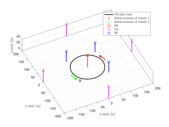
Figure 1: Vehicle trajectories and common map of the environment (1 BS, 4 VAs, and 4 SPs). Two vehicles are initially located at opposite sides of $[0,0,0]~{}\mathrm{m}$, and move along with counterclockwise. Two vehicles have observed same objects (i.e., explored area) when $k$ is about 40.

VI-A Simulation Setup

We consider a three dimensional (3D) vehicular network where two moving vehicles are on a circular road with a BS, four VAs, and four SPs as shown in Fig. 1. Such a scenario is sufficiently representative to demonstrate the efficacy of the proposed PHD filter and map fusion, though actual performance in localization and mapping will depend on the chosen scenario. The details of the scenario are shown and available in [43]. During $K=40$ time steps, the vehicle states are evolved with the dynamics model (1) as discussed in Section III-A, with

$$\bm{\upsilon}(\mathbf{s}^{(n)}_{k-1})=\mathbf{s}^{(n)}_{k-1}+\left[\begin{array}[]{c}\frac{\zeta^{(n)}_{k-1}}{\rho^{(n)}_{k-1}}\left(\sin(\alpha^{(n)}_{k-1}+\rho^{(n)}_{k-1}\Delta)-\sin\alpha^{(n)}_{k-1}\right)\\ \frac{\zeta^{(n)}_{k-1}}{\rho^{(n)}_{k-1}}\left(-\cos(\alpha^{(n)}_{k-1}+\rho^{(n)}_{k-1}\Delta)+\cos\alpha^{(n)}_{k-1}\right)\\ 0\\ \rho^{(n)}_{k-1}\Delta\\ \mathbf{0}_{3}\end{array}\right],$$ (43)

where $\mathbf{0}_{\psi}$ denotes a column vector of $\psi$ zeros, $\Delta$ is the sampling time and $\mathbf{q}_{k}$ denotes the process noise, modeled as zero-mean Gaussian with covariance $\mathbf{Q}=\mathrm{diag}[\sigma_{x}^{2},\sigma_{y}^{2},0,\sigma^{2}_{\alpha},\mathbf{0}_{2},\sigma^{2}_{B}]$. The vehicles are initialized as $\mathbf{s}^{(1)}_{0}=[70.7285~{}\text{m},0~{}\text{m},0~{}\text{m},\pi/2~{}\text{rad},22.22~{}\text{m/s},\pi/10~{}\text{rad/s},300~{}\text{m}]^{\text{T}}$ and $\mathbf{s}^{(2)}_{0}=[-70.7285~{}\text{m}\mathchar 44\relax\penalty 00~{}\text{m}\mathchar 44\relax\penalty 00~{}\text{m}\mathchar 44\relax\penalty 0\pi/2~{}\text{rad}\mathchar 44\relax\penalty 0-22.22~{}\text{m/s}\mathchar 44\relax\penalty 0\pi/10~{}\text{rad/s}\mathchar 44\relax\penalty 0300~{}\text{m}]^{\text{T}}$. The time interval $\Delta$ is set to $0.5$ s. The process noise standard deviations are set to $\sigma_{x}=0.2$ m, $\sigma_{y}=0.2$ m, $\sigma_{\alpha}=0.001$ rad, and $\sigma_{B}=0.2$ m. The initial prior of the vehicle state follows zero-mean Gaussian distribution with $0.3$ m standard deviation for both x and y location, $0.3$ rad for the vehicle heading, $0.3$ m the bias. The longitudinal velocity $\zeta^{(n)}_{k}$, rotational velocity $\rho^{(n)}_{k}$ are assumed to be known. The measurement covariance matrix $\bm{\Sigma}^{(n)}_{k,l}$ is diagonal, and is set to $\text{diag}(10^{-2}~{}\text{m}^{2},10^{-4}~{}\text{rad}^{2},10^{-4}~{}\text{rad}^{2},10^{-4}~{}\text{rad}^{2})$. To mitigate the effect of the errors in the CKF (due to the non-invertible nonlinearity), we replace the measurement $\bm{\Sigma}^{(n)}_{k,l}$ with $\bm{\Sigma}_{\textrm{PHD}}=9\times\bm{\Sigma}^{(n)}_{k,l}$ in (50) for the birth process, and in the CKF update of Algorithm 1 for the map correction. A BS is located at $[0,0,40]^{\text{T}}$ m. Four VAs are located at $[200,0,40]^{\text{T}}$ m, $[-200,0,40]^{\text{T}}$ m, $[0,200,40]^{\text{T}}$ m, $[0,-200,40]^{\text{T}}$ m. Four SPs are located at $[65,65,z_{\text{SP}}]^{\text{T}}$ m, $[-65,65,z_{\text{SP}}]^{\text{T}}$ m, $[-65,-65,z_{\text{SP}}]^{\text{T}}$ m, and $[65,-65,z_{\text{SP}}]^{\text{T}}$ m, where $z_{\text{SP}}\sim\mathcal{U}(0,40)$. The SPs are only visible when the distance between the SP and vehicle is within the FoV range $r_{\text{FoV}}=50~{}\text{m}$, while VAs are always visible. The detection probability $p_{\text{D}}$ is set to 0.9 within the FOV. In the Gaussian representation of the birth process (18), we consider the birth weight $\gamma_{b,k}^{i,j(\mathbf{z})}(m)=1.5\times 10^{-5}$ for $m=\{\textrm{VA,SP}\}$. For the clutter intensity $c(\mathbf{z})$, we consider the average of the number of clutter measurements (following Poisson distribution) $\lambda=1$, and the maximum sensing range $R_{\max}=200$ m, so $c(\mathbf{z})=\lambda/(4R_{\max}\pi^{4})$. We utilized the pruning and merging in [37, Table II], and also used its parameter notations as follows: truncation threshold $T$; merging threshold $U$; and maximum allowable number of Gaussians $J_{\max}$. We considered $T=10^{-4}$, $U=49$, and $J_{\max}=50$. The object detection parameters are set to as follows: the VA detection threshold $T_{\text{VA}}=0.7$; the SP detection threshold $T_{\text{SP}}=0.55$. We consider an asynchronous map fusion where each vehicle communicates with the BS every 4 time steps, with vehicle 1 starting at time 10 and vehicle 2 at time 12. Each vehicle’s state was represented by $I=2000$ particles, and simulation results were obtained by averaging over $N_{\mathrm{mc}}=20$ Monte Carlo runs (we observed no significant performance differences when increasing $N_{\mathrm{mc}}$ from 10 to 20). Complete source code is available at https://github.com/HyowonKim-P1/5GmmWavePHDFilterMapFusion.

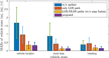
Figure 2: MAEs and RMSE bars of the vehicle states (vehicle location, clock bias, and heading).

VI-B Performance Metric

To demonstrate the efficacy of the method and support the contributions of this paper described in Section I. The performances of the vehicle state estimation and the mapping of the environment are evaluated, over all Monte Carlo runs during the steady-state operation, which was determined to be after $k=20$. For the vehicle state estimation, we compute the mean absolute error (MAE) on each component (location, clock bias, heading), along with root mean square error (RMSE) bars. For the mapping, we compute the average of the generalized optimal subpattern assignment (GOSPA) distance [44], as follows (removing the time index $k$ and the source type index $m$). We denote $\mathcal{L}=\{(\mathbf{x}_{1},m_{1}),\ldots,(\mathbf{x}_{M},m_{M})\}$ and $\hat{\mathcal{L}}=\{(\hat{\mathbf{x}}_{1},\hat{m}_{1}),\ldots,(\hat{\mathbf{x}}_{\hat{M}},\hat{m}_{\hat{M}})\}$ by the set of sources (of type $m$ at time $k$) and its estimated set, respectively. The FoV was not considered in the GOSPA distance metric in order to evaluate the map fusion performance. Then, the GOSPA is defined as

$$d^{(q_{c},q_{a},q_{p})}_{\text{GOSPA}}=\bigg{(}\min\limits_{\mathcal{M}\in\Pi_{|\hat{\mathcal{L}}|}}\sum_{e=1}^{M}d^{q_{c}}(\hat{\mathbf{x}}_{e},\hat{\mathbf{x}}_{\mathcal{M}(e)})+\frac{q_{c}^{q_{p}}}{q_{a}}(\hat{M}-M)\bigg{)}^{\frac{1}{q_{p}}},$$ (44)

where $\Pi_{\star}$ indicates the permutations of set $\star$, cut off distance $q_{c}=20$, $q_{a}=2$, power parameter $q_{p}=2$, and $d^{q_{c}}(\mathbf{x}_{e},\hat{\mathbf{x}}_{\mathcal{M}(e)})=\min(\lVert\hat{\mathbf{x}_{e}}-\hat{\mathbf{x}}_{\mathcal{M}(e)}\rVert,q_{c})$.

VI-C Results and Discussions

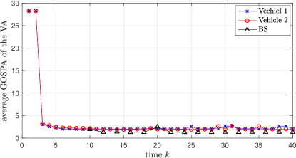
(a)

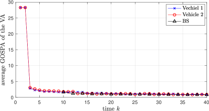
(b)

Figure 3: Average GOSPA of the VA for (a) map fusion per vehicle and uplink transmission to the BS (b) map fusion per vehicle and uplink transmission to the BS as well as downlink transmission to the vehicles.

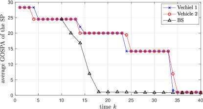
(a)

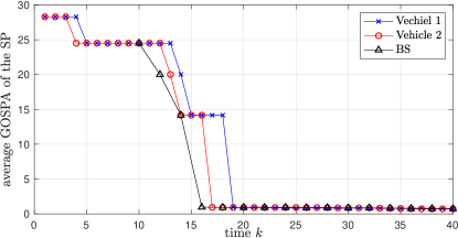
(b)

Figure 4: Average GOSPA of the SP for (a) map fusion per vehicle and uplink transmission to the BS (b) map fusion per vehicle and uplink transmission to the BS as well as downlink transmission to the vehicles.

VI-C1 Vehicle tracking

Fig. 2 shows the MAE and RMSE bars of the estimated vehicle location, clock bias, and heading with respect to (w.r.t.) the four cases as follows: i) only performing the vehicle state prediction without the update step; ii) using only the measurement from the LOS path; iii) proposed PHD filter for positioning and mapping per vehicle from Section IV; and iv) proposed PHD filtering and map fusion from Section V. In case i), the accuracy of the estimated vehicle state gradually increases and demonstrates the need for measurements in the considered scenario. Case ii) can be considered a best-case, without any objects in the environment and a clear LOS at all times. We see that the performance is significantly improved compared to case i). In case iii), the performance is much better than case ii) showing the benefit of NLOS information, even with unknown source association. In case iv), despite the reduced map diversity (see Section V-C) the performance is not reduced compared to case iii), but there are only marginal performance gains either. This is due to the specific scenario, where the vehicles independently are able to localize themselves well. In addition, since the VAs are always visible for both vehicles and can be mapped accurately, the main cooperative localization gain can come from the SPs. Since SPs have variable detection probability, they provide only limited information for the vehicles’ positions.

VI-C2 Mapping

Fig. 3 shows the average GOSPA of the VA map, with Fig. 3a considering the case of the local PHD filter and map fusion at the BS, but no downlink transmission, while Fig. 3b presents the performance of the proposed PHD filter and map fusion with downlink transmission. Comparing Fig. 3a and Fig. 3b, there is only a small, little or no benefit the downlink transmissions, as both vehicles have all VAs in their FoV at all time. This is in contrast to the SP map, where Fig. 4 reports the GOSPA results. In Fig. 4a, we see that the GOSPA per vehicle goes down as they move in the environment. The GOSPA at the BS is reduced faster, as it can benefit from the information of all vehicles. In Fig. 4b, we note that when the BS sends back the map to the vehicles over the downlink, each vehicle can benefit from the measurements of the other vehicle, so that the GOSPA is reduced faster on the vehicle maps as well.

VII Conclusions

It is expected that the framework of cooperative positioning and mapping with the proposed multiple-model PHD filter and map fusion is essential for vehicular positioning. In this paper, we proposed a multiple-model PHD filter and map fusion for cooperative positioning and mapping in vehicular networks with 5G mmWave communication links. The environment comprises a single BS, multiple vehicles, and different types of objects (small scattering objects and large reflecting surfaces). The challenges of the mapping such as the number of objects, object type, and their position were dealt with the proposed PHD filter. In addition, asynchronous map transmission to the BS is solved by the proposed map fusion method. From the results, it is confirmed that our PHD filter can handle the challenges of the mapping and vehicle state estimation simultaneously. We also confirmed that the proposed map fusion using map information of other vehicles significantly improves the mapping performance.

Appendix A Geometric Relations

In the relation between the observations (3), the state of the vehicle and the map depend on the origin of the measurement. We distinguish between 3 different cases.

A-A Source is the BS

For the LOS path between BS and vehicle, we have the following relations: $\tau=\|\mathbf{x}_{\text{BS}}-\mathbf{v}_{k}\|/c+B$, where $c$ denotes the speed of light; $\phi_{0}^{\textrm{az}}=\arctan\left({y_{k}}/{x_{k}}\right)$, $\phi_{0}^{\textrm{el}}=\arcsin\left(({z_{k}-z_{\textrm{BS}}})/({\|\mathbf{v}_{k}-\mathbf{x}_{\mathrm{BS}}\|})\right)$, where we assume $\operatorname{arctan2}$ is used; We remind that the DOA is measured in the local frame of reference of the vehicle, so that the vehicle orientation must be accounted for: $\theta_{0}^{\textrm{az}}=\pi+\arctan\left({y_{k}}/{x_{k}}\right)-\alpha_{k}$, $\theta_{0}^{\textrm{el}}=\arcsin\left(({z_{\textrm{BS}}-z_{k}})/({\|\mathbf{x}_{\mathrm{BS}}-\mathbf{v}_{k}\|})\right)$, since the DOA elevation measurement does not depend on the vehicle orientation.

A-B Source is a reflecting surface

Each reflecting surface can be parameterized by a fixed virtual anchor (VA) location $\mathbf{x}_{\mathrm{VA}}$, obtained by mirroring the BS with respect to the surface. Between a virtual anchor $\mathbf{x}_{\text{VA}}$ and the user’s position $\mathbf{v}_{k}$, the incidence point of the specular reflection on the reflecting surface is given by the point where the straight line between the VA and vehicle crosses the reflecting surface

$$\mathbf{x}_{s}=\mathbf{x}_{\text{VA}}+\frac{(\mathbf{f}-\mathbf{x}_{\text{VA}})^{\mathrm{T}}\mathbf{u}}{(\mathbf{v}_{k}-\mathbf{x}_{\text{VA}})^{\mathrm{T}}\mathbf{u}}(\mathbf{v}_{k}-\mathbf{x}_{\text{VA}}).$$ (45)

Here, $\mathbf{u}=(\mathbf{x}_{\text{BS}}-\mathbf{x}_{\text{VA}})/\|(\mathbf{x}_{\text{BS}}-\mathbf{x}_{\text{VA}})\|$ and $\mathbf{f}=(\mathbf{x}_{\text{BS}}+\mathbf{x}_{\text{VA}})/2$. Note that this allows to find explicit expressions of $\mathbf{x}_{s}$ that only depend on $\mathbf{x}_{\text{VA}}$, $\mathbf{x}_{\text{BS}}$, and $\mathbf{v}_{k}$ (not shown). Conversely, the location of a VA can be expressed as a function of the incidence point

$$\mathbf{x}_{\mathrm{VA}}=\mathbf{v}_{k}+(\|\mathbf{v}_{k}-\mathbf{x}_{s}\|+\|\mathbf{x}_{\mathrm{BS}}-\mathbf{x}_{s}\|)\frac{\mathbf{x}_{s}-\mathbf{v}_{k}}{\|\mathbf{x}_{s}-\mathbf{v}_{k}\|}.$$ (46)

Next, we state the relations between the channel parameters $\tau$, $\bm{\theta}=[\theta^{\text{el}},\theta^{\text{az}}]^{\mathrm{T}}$, and $\bm{\phi}=[\phi^{\text{el}},\phi^{\text{az}}]^{\mathrm{T}}$ and the system state: $\tau=\|\mathbf{x}_{\mathrm{VA}}-\mathbf{v}_{k}\|/c+B$. This is equivalent to $\tau=\|\mathbf{x}_{\mathrm{BS}}-\mathbf{x}_{s}\|/c+\|\mathbf{x}_{s}-\mathbf{v}_{k}\|/c+B$; $\phi^{\textrm{az}}=\arctan\left({y_{\textrm{s}}}/{x_{\textrm{s}}}\right)$ and $\phi^{\textrm{el}}=\arcsin\left(({z_{\textrm{s}}-z_{\textrm{BS}}})/({\|\mathbf{x}_{\textrm{s}}-\mathbf{x}_{\mathrm{BS}}\|})\right)$; and $\theta^{\textrm{az}}=\arctan\left(({y_{\textrm{VA}}-y_{k}})/({x_{\textrm{VA}}-x_{k}})\right)-\alpha_{k}$ and $\theta^{\textrm{el}}=\arcsin\left(({z_{\textrm{VA}}-z_{k}})/({\|\mathbf{x}_{\textrm{VA}}-\mathbf{v}_{k}\|})\right)$.

A-C Source is a small object

For small objects (SPs), the relations are largely a special case of the VAs. We here only note the differences, considering an SP with location $\mathbf{x}_{\text{SP}}$: $\tau=\|\mathbf{x}_{\mathrm{SP}}-\mathbf{x}_{\mathrm{BS}}\|/c+\|\mathbf{x}_{\mathrm{SP}}-\mathbf{v}_{k}\|/c+B$; $\phi^{\textrm{az}}=\arctan\left({y_{\textrm{SP}}}/{x_{\textrm{SP}}}\right)$ and $\phi^{\textrm{el}}=\arcsin\left(({z_{\textrm{SP}}-z_{\textrm{BS}}})/({\|\mathbf{x}_{\textrm{SP}}-\mathbf{x}_{\mathrm{BS}}\|})\right)$; and $\theta^{\textrm{az}}=\arctan\left(({y_{\textrm{SP}}-y_{k}})/({x_{\textrm{SP}}-x_{k}})\right)-\alpha_{k}$ and $\theta^{\textrm{el}}=\arcsin\left(({z_{\textrm{SP}}-z_{k}})/({\|\mathbf{x}_{\textrm{SP}}-\mathbf{v}_{k}\|})\right)$.

Appendix B Proof of Expected Likelihood (15)

From (8), we find $f(\mathcal{X}|\mathbf{s}_{0:k}^{i},\mathcal{Z}_{1:k-1})\propto\prod_{(\mathbf{x},m)\in\mathcal{X}}D_{k|k-1}^{i}(\mathbf{x},m)$ under a PPP prior approximation, while with $\mathcal{Z}_{k}=\{\mathbf{z}_{1},\ldots,\mathbf{z}_{|\mathcal{Z}_{k}|}\}$, the function $f(\mathcal{Z}_{k}|\mathcal{X},\mathbf{s}_{0:k}^{i},\mathcal{Z}_{1:k-1})$ can be expressed as [38, eq. (13)]

$$f(\mathcal{Z}_{k}|\mathcal{X},\mathbf{s}_{0:k}^{i},\mathcal{Z}_{1:k-1})=\sum_{\mathcal{U}\uplus\mathcal{X}_{1}\ldots\uplus\mathcal{X}_{|\mathcal{Z}_{k}|}=\mathcal{X}}\prod_{(\mathbf{x},m)\in\mathcal{U}}(1-p_{\text{D}}^{i}(\mathbf{x},m))\times\prod_{r=1}^{|\mathcal{Z}_{k}|}\ell(\mathbf{z}_{r}|\mathcal{X}_{r},\mathbf{s}_{k}^{i}),$$ (47)

where $\uplus$ denotes the disjoint union and [38, eq. (14)]

$$\ell(\mathbf{z}_{r}|\mathcal{X}_{r},\mathbf{s}_{k}^{i})=\begin{cases}p_{\text{D}}^{i}(\mathbf{x},\mathbf{s}_{k}^{i},m)f(\mathbf{z}_{r}|\mathbf{x},\mathbf{s}_{k}^{i},m)&\mathcal{X}_{r}=\{(\mathbf{x},m)\},\\ c(\mathbf{z}_{r})&X_{r}=\emptyset,\\ 0&\text{else}.\end{cases}$$ (48)

Introducing a PPP density $q(\mathcal{U})\propto\prod_{(\mathbf{x},m)\in\mathcal{U}}(1-p_{\text{D}}^{i}(\mathbf{x},m))D_{k|k-1}^{i}(\mathbf{x},m)$ and making use of the fact that $\int\sum_{\mathcal{X}\uplus\mathcal{Y}=\mathcal{U}}f(\mathcal{X})g(\mathcal{Y})\delta\mathcal{U}=\int f(\mathcal{X})\delta\mathcal{X}\int g(\mathcal{Y})\delta\mathcal{Y},$ we immediately find that

$$f(\mathcal{Z}_{k}|\mathbf{s}_{0:k}^{i},\mathcal{Z}_{1:k-1}) =\int f(\mathcal{Z}_{k}|\mathcal{X},\mathbf{s}_{0:k}^{i},\mathcal{Z}_{1:k-1})f(\mathcal{X}|\mathbf{s}_{0:k}^{i},\mathcal{Z}_{1:k-1})\delta\mathcal{X}$$

$$\propto\prod_{r=1}^{|\mathcal{Z}_{k}|}\int\ell(\mathbf{z}_{r}|\mathcal{X}_{r},\mathbf{s}_{k}^{i})D_{k|k-1}^{i}(\mathcal{X}_{r})\delta\mathcal{X}_{r}$$ (49)

$$=\prod_{\mathbf{z}\in\mathcal{Z}_{k}}(c(\mathbf{z})+\sum_{m}\int p_{\text{D}}^{i}(\mathbf{x},\mathbf{s}_{k}^{i},m)f(\mathbf{z}|\mathbf{x},\mathbf{s}_{k}^{i},m)D_{k|k-1}^{i}(\mathbf{x},m)\text{d}\mathbf{x}),$$

where the last step follows from substitution of (48) and the definition of set integrals (6).

Appendix C Implementation of Birth Process

Here, we introduce the detailed implementation of the birth process (18). The mean $\mathbf{x}^{i,j(\mathbf{z})}_{b,k}(m)$ and covariance $\mathbf{P}^{i,j(\mathbf{z})}_{b,k}(m)$ corresponding to each measurement $\mathbf{z}$ are inversely estimated by using sigma point principle of the CKF [40], details of which are described in Appendix C-A For propagating the cubature points, the inverse of the nonlinear function in (4) is required, which in general is not defined (since a vehicle state gives rise to a noise-free measurement, but a noisy measurement may not correspond to a vehicle state). Thus, the cubature points are propagated using a simple optimization method, described in Appendix C-B. For simplification, all indices are dropped except for the source type $m$.

C-A Mean and Covariance Estimation

The mean $\mathbf{x}(m)$ and covariance $\mathbf{P}(m)$ are approximated by the following steps:

1. Factorize the covariance matrix of the measurement noise (i.e., $\bm{\Sigma}^{(n)}_{k,l}$ of (4))

   $$\bm{\Sigma}=\mathbf{G}\mathbf{G}^{\mathrm{T}}.$$ (50)

2. Evaluate the cubature point $(c=1,...,2d_{\mathbf{z}})$

   $$\mathbf{z}_{c}=\mathbf{G}\delta_{\mathbf{z},c}+\mathbf{z},$$ (51)

   where $d_{\mathbf{z}}=\dim({\mathbf{z}})$ and $\delta_{\mathbf{z},c}=\sqrt{d_{\mathbf{z}}}[1]_{\mathbf{z},c}$. $[1]_{\mathbf{z},c}$ is defined as the $c$-th column vector of the matrix $[\mathbf{I}_{d_{\mathbf{z}},d_{\mathbf{z}}},-\mathbf{I}_{d_{\mathbf{z}},d_{\mathbf{z}}}]\in\mathbb{R}^{d_{\mathbf{z}}\times 2d_{\mathbf{z}}}$, where $\mathbf{I}_{d_{\mathbf{z}},d_{\mathbf{z}}}\in\mathbb{R}^{d_{\mathbf{z}}\times d_{\mathbf{z}}}$ is the identity matrix.

3. Evaluate the propagated cubature point $\mathbf{x}_{c}(m)\approx\mathbf{h}^{-1}(\mathbf{z}_{c}|\mathbf{s},m)$ with the iterative maximum-likelihood estimation (explained further in Appendix C-B).

4. Evaluate birth mean $\mathbf{x}(m)=\frac{1}{2d_{\mathbf{z}}}\sum_{c=1}^{2d_{\mathbf{z}}}\mathbf{x}_{c}(m)$ and covariance $\mathbf{P}(m)=\frac{1}{2d_{\mathbf{z}}}\sum_{c=1}^{2d_{\mathbf{z}}}\mathbf{x}_{c}(m){\mathbf{x}_{c}{(m)}}^{\mathrm{T}}-\mathbf{x}{(m)}{\mathbf{x}{(m)}}^{\mathrm{T}}$.

C-B Simple Optimization Problem for Propagated Cubature Point

For estimating the propagated cubature point $\mathbf{x}_{c}{(m)}$ of step 3) in Appendix C-A, we formulate an optimization problem as

$$\operatorname*{minimize}_{\mathbf{x}}\big{(}\mathbf{h}(\mathbf{x},\mathbf{s},m)-\mathbf{z}_{c}\big{)}^{\mathrm{T}}\bm{\Sigma}^{-1}\big{(}\mathbf{h}(\mathbf{x},\mathbf{s},m)-\mathbf{z}_{c}\big{)},$$ (52)

where $\mathbf{h}(\mathbf{x},\mathbf{s},m)$ is the observation function for the source type $m$ with the source location $\mathbf{x}$ and vehicle state $\mathbf{s}$, and $\mathbf{z}_{c}\in\mathbb{R}^{d_{z}}$ is the evaluated cubature point in (51). Note that the used function $\mathbf{h}(\cdot)$ are determined with respect to the source type $m$, which were described in Appendix A. However, (52) does not admit a closed-form solution, and an optimal point is determined in a iterative manner. The optimum point at the iteration $\epsilon+1$ is designed as $\bar{\mathbf{x}}_{\epsilon+1}{(m)}=(1-\eta)\bar{\mathbf{x}}_{\epsilon}{(m)}+\eta\tilde{\mathbf{x}}_{\epsilon+1}{(m)}$, where the design parameter $\eta$ is set to 0.2, and the initial point $\bar{\mathbf{x}}_{0}$ is obtained by geometric relations in Appendix A. $\tilde{\mathbf{x}}_{\epsilon+1}$ is calculated as $\tilde{\mathbf{x}}_{\epsilon+1}=\operatorname*{argmin}_{\mathbf{x}}{\mathbf{A}(\mathbf{x},m)}^{\mathrm{T}}\bm{\Sigma}^{-1}\mathbf{A}(\mathbf{x},m)$, where $\mathbf{A}(\mathbf{x},m)$ is denoted by $\mathbf{A}(\mathbf{x},m)=\mathbf{H}(\bar{\mathbf{x}}_{\epsilon},\mathbf{s},m)(\mathbf{x}-\bar{\mathbf{x}}_{\epsilon})+\mathbf{h}(\bar{\mathbf{x}}_{\epsilon},\mathbf{s},m)-\mathbf{z}_{c}$, where $\mathbf{H}(\bar{\mathbf{x}}_{\epsilon},\mathbf{s},m)\in\mathbb{R}^{5\times 3}$ is a Jacobian matrix, and is calculated by the finite difference method [45]. The difference is set to $10^{-3}$. The iterative method is performed until the cost (52) increases, and then $\mathbf{x}_{c}$ is determined.

Appendix D Pseudo-code for Map Update

The pseudo-code is provided in Algorithms 1–3.

Algorithm 1 Map Correction

Input: $\{D^{i}_{k|k-1}(\mathbf{x},m)\}_{i=1}^{I}~{}~{}\forall m,$ where $D^{i}_{k|k-1}(\mathbf{x},m)$ $=$ $\{\gamma^{i,j}_{k|k-1}(m),\mathbf{x}^{i,j}_{k|k-1}(m),\mathbf{P}^{i,j}_{k|k-1}(m)\}_{j=1}^{J^{i,(m)}_{k|k-1}}$, $\{\mathbf{s}_{k|k-1}^{i},\omega_{k|k-1}^{i}\}_{i=1}^{I},\mathcal{Z}_{k}$.
Output: $\{D^{i}_{k|k}(\mathbf{x},m)\}_{i=1}^{I}~{}~{}\forall m,$ where $D^{i}_{k|k}(\mathbf{x},m)=\{\gamma^{i,j}_{k|k}(m),\mathbf{x}^{i,j}_{k|k}(m),\mathbf{P}^{i,j}_{k|k}(m)\}_{j=1}^{J^{i,(m)}_{k|k}}$.

1:for $i=1$ to $I$ do (particle sample)

2:    Compute PHD update components by CKF (described in Algorithm 2)

3:    PHD update (described in Algorithm 3)

4:end for

Algorithm 2 Compute PHD update components by CKF

1:for $m=\{\text{BS,VA,SP}\}$ do (source type)

2:    for $j=1$ to $J^{i}_{k|k-1}(m)$ do

3:        $\mathbf{P}^{i,j}_{k|k-1}(m)=\mathbf{G}^{i,j}_{k}(m){\mathbf{G}^{i,j}_{k}(m)}^{\text{T}}$

4:        for $c=1$ to $2d_{\mathbf{x}}$ do

5:           $\mathbf{X}^{i,j}_{c,k}(m)=\mathbf{x}^{i,q}_{k|k-1}(m)+\mathbf{G}^{i,j}_{k}(m)\delta_{\mathbf{x},c}$, $\mathbf{Z}_{c,k}^{i,j}(m)=\mathbf{h}_{k}(\mathbf{x}^{i,j}_{k|k-1}(m),\mathbf{s}^{i}_{k},m)$

6:        end for

7:        ${\mathbf{Z}}^{i,j}_{k}(m)=\frac{1}{2d_{\mathbf{x}}}\sum_{c=1}^{2d_{\mathbf{x}}}\mathbf{Z}^{i,j}_{c,k}(m)$

8:        $\mathbf{S}^{i,j}_{\mathbf{z}\mathbf{z},k}(m)=\frac{1}{2d_{\mathbf{x}}}\sum_{c=1}^{2d_{\mathbf{x}}}\mathbf{Z}_{c,k}^{i,j}(m){\mathbf{Z}_{c,k}^{i,j}(m)}^{\text{T}}-{\mathbf{Z}}^{i,j}_{k}(m){{\mathbf{Z}}^{i,j}_{k}(m)}^{\text{T}}+\bm{\Sigma}_{k,l}$

9:        if $m=\{\text{VA,SP}\}$ then

10:           ${\mathbf{X}}^{i,j}_{k}(m)=\frac{1}{2d_{\mathbf{x}}}\sum_{c=1}^{2d_{\mathbf{x}}}\mathbf{X}^{i,j}_{c,k}(m)$

11:           $\mathbf{S}^{i,j}_{\mathbf{x}\mathbf{z},k}(m)=\frac{1}{2d_{\mathbf{x}}}\sum_{c=1}^{2d_{\mathbf{x}}}\mathbf{X}_{c,k}^{i,j}(m){\mathbf{Z}_{c,k}^{i,j}(m)}^{\text{T}}-{\mathbf{X}}^{i,j}_{k}(m){{\mathbf{Z}}^{i,j}_{k}(m)}^{\text{T}}$

12:           $\mathbf{K}^{i,j}_{k}(m)=\mathbf{S}^{i,j}_{\mathbf{x}\mathbf{z},k}(m){\mathbf{S}^{i,j}_{\mathbf{z}\mathbf{z},k}(m)}^{-1}$

13:           $\mathbf{P}^{i,j}_{k|k}(m)=\mathbf{P}^{i,j}_{k|k-1}(m)-\mathbf{K}^{i,j}_{k}(m)\mathbf{S}^{i,j}_{\mathbf{z}\mathbf{z},k}(m){\mathbf{K}^{i,j}_{k}(m)}^{\text{T}}$

14:        end if

15:    end for

16:    $q=0$

17:    for $\mathbf{z}\in\mathcal{Z}_{k}$ do

18:        $q=q+1$

19:        for $j=1$ to $J^{i}_{k|k-1}(m)$ do

20:           if $j=j(\mathbf{z})$ then

21:               $\mu^{i,qJ^{i}_{k|k-1}(m)+j}_{k}(m)=\gamma^{i,j}_{k|k-1}(m)$

22:           else ($j\neq j(\mathbf{z})$)

23:               $\mu^{i,qJ^{i}_{k|k-1}(m)+j}_{k}(m)=p^{i,j}_{D,k}(m)\gamma^{i,j}_{k|k-1}(m)\mathcal{N}(\mathbf{z};\mathbf{h}_{k}(\mathbf{x}^{i,j}_{k|k-1}(m),\mathbf{s}_{k}^{i},m),\mathbf{S}_{\mathbf{z}\mathbf{z},k}^{i,j}(m))$

24:           end if

25:        end for

26:    end for

27:end for

Algorithm 3 PHD update

for $m=\{\text{VA,SP}\}$ do (source type)

    for $j=1$ to $J^{i}_{k|k-1}(m)$ do (missed detections)

        if $j$ is a birth then

           $\gamma^{i,j}_{k|k}(m)=0$, $\mathbf{x}^{i,j}_{k|k}(m)=\mathbf{x}^{i,j}_{k|k-1}(m)$, $\mathbf{P}^{i,j}_{k|k}(m)=\mathbf{P}^{i,j}_{k|k-1}(m)$

        else ($j$ is not a birth)

           $\gamma^{i,j}_{k|k}(m)=\{1-p^{i,j}_{D,k}(m)\}\gamma^{i,j}_{k|k-1}(m)$, $\mathbf{x}^{i,j}_{k|k}(m)=\mathbf{x}^{i,j}_{k|k-1}(m)$, $\mathbf{P}^{i,j}_{k|k}(m)=\mathbf{P}^{i,j}_{k|k-1}(m)$

        end if

    end for

    $q=0$;

    for $\mathbf{z}\in\mathcal{Z}_{k}$ do (detections)

        $q=q+1$

        for $j=1$ to $J^{i}_{k|k-1}(m)$ do

           if $j=j(\mathbf{z})$ then

               $\mathbf{x}^{i,qJ^{i}_{k|k-1}(m)+j}_{k|k}(m)=\mathbf{x}^{i,j}_{k|k-1}(m)$, $\mathbf{P}^{i,qJ^{i}_{k|k-1}(m)+j}_{k|k}(m)=\mathbf{P}^{i,j}_{k|k-1}(m)$

           else ($j\neq j(\mathbf{z})$)

               $\mathbf{x}^{i,qJ^{i}_{k|k-1}(m)+j}_{k|k}(m)=\mathbf{x}^{i,j}_{k|k-1}(m)+\mathbf{K}^{i,j}_{k}(m)(\mathbf{z}-{\mathbf{Z}_{k}}^{i,j}(m))$

               $\mathbf{P}^{i,qJ^{i}_{k|k-1}(m)+j}_{k|k}(m)=\mathbf{P}^{i,j}_{k|k}(m)$

           end if

           $\gamma^{i,qJ^{i}_{k|k-1}(m)+j}_{k|k}(m)=\mu^{i,qJ^{i}_{k|k-1}(m)+j}_{k}(m)/(c(\mathbf{z})+\sum_{m^{\prime}=\{\text{BS,VA,SP}\}}\sum_{j^{\prime}=1}^{J^{i}_{k|k-1}(m^{\prime})}$       $\mu^{i,qJ^{i}_{k|k-1}(m^{\prime})+j^{\prime}}_{k}(m^{\prime}))$

        end for

    end for

    $J^{i}_{k|k}(m)=(q+1)J^{i}_{k|k-1}(m)$

end for

$\mathbf{x}^{i,j}_{k|k}(\text{BS})=\mathbf{x}^{i,j}_{k|k-1}(\text{BS}),\mathbf{P}^{i,j}_{k|k}(\text{BS})=\mathbf{P}^{i,j}_{k|k-1}(\text{BS}),\gamma^{i,j}_{k|k}(\text{BS})=1,J^{i}_{k|k}(\text{BS})=1$

References

- [1] H. Wymeersch, G. Seco-Granados, G. Destino, D. Dardari, and F. Tufvesson, “5G mm-Wave positioning for vehicular networks,” IEEE Wireless Commun., vol. 24, no. 6, pp. 80–86, Dec. 2018.
- [2] A. Shahmansoori, G. E. Garcia, G. Destino, G. Seco-Granados, and H. Wymeersch, “Position and orientation estimation through millimeter-wave MIMO in 5G systems,” IEEE Trans. Wireless Commun., vol. 17, no. 3, pp. 1822–1835, Mar. 2018.
- [3] K. Witrisal et al., “High-accuracy localization for assisted living: 5G systems will turn multipath channels from foe to friend,” IEEE Signal Process. Mag., vol. 33, no. 2, pp. 59–70, Mar. 2016.
- [4] J. Palacios, G. Bielsa, P. Casari, and J. Widmer, “Single-and multiple-access point indoor localization for millimeter-wave networks,” IEEE Trans. Wireless Commun., vol. 18, no. 3, pp. 1927–1942, Feb. 2019.
- [5] H. Wymeersch, N. Garcia, H. Kim, G. Seco-Granados, S. Kim, F. Wen, and M. Fröhle, “5G mmWave downlink vehicular positioning,” in Proc. IEEE Global Commun. Conf. (GLOBECOM), Abu Dhabi, UAE, Dec. 2018, pp. 206–212.
- [6] H. Durrant-Whyte and T. Bailey, “Simultaneous localization and mapping: Part I,” IEEE Robot. Autom. Mag., vol. 13, no. 2, pp. 99–110, Jun. 2006.
- [7] T. Bailey and H. Durrant-Whyte, “Simultaneous localization and mapping (SLAM): Part II,” IEEE Robot. Autom. Mag., vol. 13, no. 3, pp. 108–117, Sep. 2006.
- [8] A. Yassin, Y. Nasser, A. Y. Al-Dubai, and M. Awad, “MOSAIC: Simultaneous localization and environment mapping using mmWave without a-priori knowledge,” IEEE Access, vol. 6, pp. 68 932–68 947, Nov. 2018.
- [9] M. Aladsani, A. Alkhateeb, and G. C. Trichopoulos, “Leveraging mmWave imaging and communications for simultaneous localization and mapping,” in Proc. 2019 IEEE Int. Conf. Acoust., Speech Signal Process. (ICASSP), Brighton, UK, May 2019, pp. 4539–4543.
- [10] J. Palacios, P. Casari, and J. Widmer, “JADE: Zero-knowledge device localization and environment mapping for millimeter wave systems,” in Proc. IEEE Int. Conf. Comput. Commun. (INFOCOM), Atlanta, GA, USA, May 2017, pp. 1–9.
- [11] J. Palacios, G. Bielsa, P. Casaril, and J. Widmer, “Communication-driven localization and mapping for millimeter wave networks,” in Proc. IEEE Int. Conf. Comput. Commun. (INFOCOM), Honolulu, HI, USA, Apr. 2018, pp. 2402–2410.
- [12] R. Mendrzik, H. Wymeersch, G. Bauch, and Z. Abu-Shaban, “Harnessing NLOS components for position and orientation estimation in 5G millimeter wave MIMO,” IEEE Trans. Wireless Commun., vol. 18, no. 1, pp. 93–107, 2018.
- [13] H. Kim, H. Wymeersch, N. Garcia, G. Seco-Granados, and S. Kim, “5G mmWave vehicular tracking,” in Proc. IEEE 52nd Asilomar Conf. Signals, Syst., Comput., Pacific Grove, CA, USA, Oct. 2018, pp. 541–547.
- [14] R. Mahler, “Multitarget Bayes filtering via first-order multi target moments,” IEEE Trans. Aerosp. Electron. Syst., vol. 39, no. 4, pp. 1152–1178, Oct. 2003.
- [15] J. Mullane, B.-N. Vo, M. D. Adams, and B.-T. Vo, “A random-finite-set approach to Bayesian SLAM,” IEEE Trans. Robot., vol. 27, no. 2, pp. 268–282, Apr. 2011.
- [16] K. Y. Leung, F. Inostroza, and M. Adams, “An improved weighting strategy for Rao-Blackwellized Probability Hypothesis Density simultaneous localization and mapping,” in Proc. 13th Int. Conf. Control, Autom. and Inf. Sci. (ICCAIS), Kwangju, Korea, Oct. 2013, pp. 103–110.
- [17] G. Battistelli, L. Chisci, and A. Laurenzi, “Random set approach to distributed multivehicle SLAM,” IFAC-PapersOnLine, vol. 50, no. 1, pp. 2457 – 2464, 2017, 20th IFAC World Congress.
- [18] H. Deusch, “Random Finite Set-Based Localization and SLAM for Highly Automated Vehicles,” Ph.D. dissertation, Universität Ulm, 2015.
- [19] H. Deusch, S. Reuter, and K. Dietmayer, “The labeled multi-Bernoulli SLAM filter,” IEEE Signal Process. Lett., vol. 22, no. 10, pp. 1561–1565, Oct. 2015.
- [20] M. Fatemi, K. Granström, L. Svensson, F. Ruiz, and L. Hammarstrand, “Poisson multi-Bernoulli mapping using Gibbs sampling,” IEEE Trans. Signal Process., vol. 65, no. 11, pp. 2814–2827, Jun. 2017.
- [21] T. Li, J. M. Corchado, and S. Sun, “On generalized covariance intersection for distributed PHD filtering and a simple but better alternative,” in Proc. 20th Int. Conf. Inf. Fusion (FUSION), Xi’an, China, Jul. 2017, pp. 1–8.
- [22] T. Li, V. Elvira, H. Fan, and J. M. Corchado, “Local-diffusion-based distributed SMC-PHD filtering using sensors with limited sensing range,” IEEE Sensors J., vol. 19, no. 4, pp. 1580–1589, 2018.
- [23] L. Gao, G. Battistelli, and L. Chisci, “Multiobject fusion with minimum information loss,” arXiv preprint arXiv:1903.04239, 2019.
- [24] S. Pasha, B.-N. Vo, H. Tuan, and W.-K. Ma, “A Gaussian mixture PHD filter for jump Markov system models,” IEEE Trans. Aerosp. Electron. Syst., vol. 45, no. 3, pp. 919–936, Jul. 2009.
- [25] R. Mendrzik, H. Wymeersch, and G. Bauch, “Joint localization and mapping through millimeter wave MIMO in 5G systems-extended version,” arXiv preprint arXiv:1804.04417, 2018.
- [26] F. Meyer, T. Kropfreiter, J. L. Williams, R. Lau, F. Hlawatsch, P. Braca, and M. Z. Win, “Message passing algorithms for scalable multitarget tracking,” Proc. IEEE, vol. 106, no. 2, pp. 221–259, 2018.
- [27] H. Blom and Y. Bar-Shalom, “The interacting multiple model algorithm for systems with Markovian switching coefficients,” IEEE Trans. Autom. Control, vol. 33, no. 8, pp. 780–783, Aug. 1988.
- [28] K. Granström and C. Lundquist, “On the use of multiple measurement models for extended target tracking,” in Proc. 16th Int. Conf. Inf. Fusion (FUSION), Istanbul, Turkey, Jul. 2013.
- [29] K. Granström, S. Reuter, D. Meissner, and A. Scheel, “A multiple model PHD approach to tracking of cars under an assumed rectangular shape,” in Proc. 17th Int. Conf. Inf. Fusion (FUSION), Salamanca, Spain, Jul. 2014.
- [30] R. Mahler, “On multitarget jump-Markov filters,” in Proc. 15th Int. Conf. Inf. Fusion (FUSION), Singapore, Jul. 2012, pp. 149–156.
- [31] S. Li, G. Battistelli, L. Chisci, W. Yi, B. Wang, and L. Kong, “Multi-sensor multi-object tracking with different fields-of-view using the lmb filter,” in Proc. 21st Int. Conf. Inf. Fusion (FUSION), Cambridge, U.K., Jul. 2018, pp. 1201–1208.
- [32] G. Li, G. Battistelli, W. Yi, and L. Kong, “Distributed multi-sensor multi-view fusion based on generalized covariance intersection,” arXiv preprint arXiv:1903.06985, 2019.
- [33] S. Thrun, W. Burgard, and D. Fox, Probabilistic Robotics (Intelligent Robotics and Autonomous Agents Series). MIT Press, 2005.
- [34] X. Rong-Li and V. Jilkov, “Survey of maneuvering target tracking: Part I. Dynamic models,” IEEE Trans. Aerosp. Electron. Syst., vol. 39, no. 4, pp. 1333–1364, Oct. 2003.
- [35] R. W. Heath, N. González-Prelcic, S. Rangan, W. Roh, and A. M. Sayeed, “An overview of signal processing techniques for millimeter wave MIMO systems,” IEEE J. Sel. Topics Signal Process., vol. 10, no. 3, pp. 436–453, Apr. 2016.
- [36] J. L. Williams, “Marginal multi-bernoulli filters: RFS derivation of MHT, JIPDA, and association-based MeMBer,” IEEE Transactions on Aerospace and Electronic Systems, vol. 51, no. 3, pp. 1664–1687, Jul. 2015.
- [37] B.-N. Vo and W.-K. Ma, “The Gaussian mixture probability hypothesis density filter,” IEEE Trans. Signal Process., vol. 54, no. 11, pp. 4091–4104, Nov. 2006.
- [38] Á. F. García-Fernández, J. L. Williams, K. Granström, and L. Svensson, “Poisson multi-Bernoulli mixture filter: Direct derivation and implementation,” IEEE Trans. Aerosp. Electron. Syst., vol. 54, no. 4, pp. 1883–1901, Aug. 2018.
- [39] B. Ristic, D. Clark, B. N. Vo, and B. T. Vo, “Adaptive target birth intensity for PHD and CPHD filters,” IEEE Transactions on Aerospace and Electronic Systems, vol. 48, no. 2, pp. 1656–1668, 2012.
- [40] I. Arasaratnam and S. Haykin, “Cubature Kalman filters,” IEEE Trans. Autom. Control, vol. 54, no. 6, pp. 1254–1269, Jun. 2009.
- [41] R. P. Mahler, “Optimal/robust distributed data fusion: a unified approach,” in Signal Processing, Sensor Fusion, and Target Recognition IX, vol. 4052, 2000, pp. 128–139.
- [42] D. W. Bunn, “A Bayesian approach to the linear combination of forecasts,” Journal of the Operational Research Society, vol. 26, no. 2, pp. 325–329, 1975.
- [43] H. Kim, K. K. Granstrom, L. Gao, G. Battistelli, S. Kim, and H. Wymeersch, “5G mmWave cooperative positioning and mapping using multi-model PHD filter and map fusion,” IEEE Dataport, 2019. [Online]. Available: http://dx.doi.org/10.21227/hyfa-fa96
- [44] A. S. Rahmathullah, A. F. García Fernández, and L. Svensson, “Generalized optimal sub-pattern assignment metric,” in Proc. 20th Int. Conf. Inf. Fusion (FUSION), Xian, China, Jul. 2017, pp. 1–8.
- [45] G. D. Smith, Numerical Solution of Partial Differential Equations: Finite Difference Methods. Oxford University Press, 1985.