Stability analysis of hierarchical tensor methods for time-dependent PDEs

Abstract

In this paper we address the question of whether it is possible to integrate time-dependent high-dimensional PDEs with hierarchical tensor methods and explicit time stepping schemes. To this end, we develop sufficient conditions for stability and convergence of tensor solutions evolving on tensor manifolds with constant rank. We also argue that the applicability of PDE solvers with explicit time-stepping may be limited by time-step restriction dependent on the dimension of the problem. Numerical applications are presented and discussed for variable coefficients linear hyperbolic and parabolic PDEs.

1 Introduction

Computing the solution of high-dimensional linear PDEs has become central to many new areas of application such as random media [47], optimal transport [54], random dynamical systems [51, 52], mean field games [9], machine learning, and functional-differential equations [50]. In an abstract setting these problems involve the computation of a function $u(t,{\bf x})$ governed by an autonomous evolution equation

$$\frac{\partial u}{\partial t}={\cal L}u,\qquad u(0,{\bf x})=u_{0}({\bf x}),$$ (1)

where $u:[0,T]\times\Omega\mapsto\mathbb{R}$ is a $d$-dimensional (time-dependent) scalar field defined in the spacial domain $\Omega\subseteq\mathbb{R}^{d}$ ($d\geq 2$), and $\cal L$ is a linear operator which may may be dependent the spacial variables, and may incorporate boundary conditions. Equation (1) is first approximated with respect to the space variables, e.g., by finite differences [46], pseudo-spectral methods [24], or Galerkin methods. To this end, let us assume for simplicity that $\Omega$ is a $d$-dimensional box, i.e., $\Omega=[0,1]^{d}$. This allows us to transform (1) into the system of ordinary differential equations

$$\frac{d{\bf u}}{dt}={\bf G}{\bf u},\qquad{\bf u}(0)={\bf u}_{0},$$ (2)

where ${\bf u}:[0,T]\rightarrow{\mathbb{R}}^{n_{1}\times n_{2}\times\cdots\times n_{d}}$ is multi-dimensional array of real numbers (the solution tensor), $\bf G$ is a finite dimensional linear operator (the discrete form of $\mathcal{L}$). The structure of $\bf G$ depends on the spacial discretization of $u(t,{\bf x})$, as well as on the tensor format utilized for $\bf u$. As is well known, any straightforward spacial discretization of (1) inevitably leads to the so-called curse of dimensionality [5]. For example, approximating $u(t,{\bf x})$ using a finite-dimensional Galerkin basis with $N$ degrees of freedom in each spacial variable yields a total number of $N^{d}$ degrees of freedom. To address the exponential growth of such degrees of freedom, the computational cost and the storage requirement, techniques such as sparse collocation [7, 11, 3, 15, 35], high-dimensional model representations (HDMR) [33, 8, 2], deep learning [4, 37, 38, 56] and hierarchical tensor methods [50, 27, 1, 6, 18, 10, 29] were recently proposed, with the most efficient one being problem-specific. For instance, if a hierarchical Tucker (HT) tensor format is utilized, then the computational complexity of approximating $u(t,{\bf x})$ roughly scales as $\mathcal{O}(d\log N)$ instead of $\mathcal{O}(N^{d})$ (tensor product discretization) [16, 31, 17, 30]. Combining the spacial discretization (2) with a discrete ODE formula for the time-stepping, such an Adams-Bashforth formula, yields a decoupling of space and time which is known as the method of lines. For instance, if we discretize (2) in time with the two-step Adams-Bashforth formula, we obtain

$${\bf u}^{k+1}={\bf u}^{k}+\frac{\Delta t}{2}{\bf G}\left(3{\bf u}^{k}-{\bf u}^{k-1}\right).$$ (3)

Of particular interest are low-rank hierarchical tensor approximations of the solution to (2). Such approximations allow us to significantly reduce the number of degrees of freedom in the representation of the solution tensor ${\bf u}(t)$, while maintaining accuracy. Low-rank tensor approximations of (2) can be constructed by using, e.g., rank-constrained temporal integration [34, 28, 13] on a (smooth) tensor manifold with constant rank [48]. Alternatively, one can utilize the fully discrete scheme (3) followed by a rank-reduction operation. To this end, suppose we are given a low-rank representation of ${\bf u}^{k}$ and ${\bf u}^{k-1}$. Computing ${\bf u}^{k+1}$ based on the scheme (3) involves addition of tensors, and the application of a linear operator. All these operations increase the tensor rank of the solution, i.e., the storage requirements. To avoid an undesirable growth of the tensor rank in time, we need to truncate ${\bf u}^{k}$ back to a tensor manifold with constant rank. This operation is essentially a nonlinear projection which can be computed, e.g., by a sequence of matricizations followed by high-order singular value decomposition (HOSVD) [16, 17, 30], or by optimization [49, 44, 45, 29, 6, 12, 43, 26].

The main objective of this paper is to study the effects of truncation onto a low-rank tensor manifold on the numerical stability of explicit linear multistep schemes such as (3). To this end, we develop a thorough analysis based on a rigorous operator framework, which allows us to determine whether rank-constrained LMM integrators are stable or not. We also argue that the applicability of PDE solvers with explicit time-stepping may be limited by time-step restriction dependent on the dimension of the spacial variable.

This paper is organized as follows. In section 2 we briefly review stability of linear multistep methods (LMM) to solve the ODE (2). To this end, we follow the excellent analysis of Reddy and Trefethen [39]. In section 3 we discuss tensor rank-reduction methods in linear multistep schemes, and study the stability of the corresponding algorithms. In section 4 we argue that the applicability of PDE solvers with explicit time-stepping may be limited by time-step restrictions dependent on the dimension of the problem. Numerical examples demonstrating the theoretical claims are presented and discussed in section 5. Finally, the main findings are summarized in section 6. We also include two brief appendices where we review classical tensor algebra and the hierarchical Tucker tensor format.

2 Explicit linear multistep methods

The numerical solution to semi-discrete form (2) can be computed with the use of any ODE solver. In preparation for an analysis of rank-truncated time stepping algorithms involving hierarchical tensors, we will follow the stability analysis of Reddy and Trefethen [39]. Their analysis follows an explicit $s$-step linear multistep method (LMM) of the form

$${{\bf u}}^{k+s}+\sum_{j=0}^{s-1}a_{j}{{\bf u}}^{k+j}=\Delta t\sum_{j=0}^{s-1}b_{j}{\bf G}{{\bf u}}^{k+j},$$ (4)

where ${\bf u}^{k}\approx{{\bf u}}(k\Delta t)$ approximates the solution to (2) at time $t_{k}=k\Delta t$ ($k=0,1,\ldots$). Upon definition of

$${\bf v}^{k+1}\begin{bmatrix}{\bf u}^{k+s}\\ {\bf u}^{k+s-1}\\ \vdots\\ {\bf u}^{k+1}\end{bmatrix}\quad\text{and}\quad{\bf L}_{\Delta t}=\begin{bmatrix}b_{s-1}\Delta t{\bf G}-a_{s-1}{\bf I}&\cdots&b_{1}\Delta t{\bf G}-a_{1}{\bf I}&b_{0}\Delta t{\bf G}-a_{0}{\bf I}\\ {\bf I}&\cdots&{\bf 0}&{\bf 0}\\ \vdots&\ddots&\vdots&\vdots\\ {\bf 0}&\cdots&{\bf I}&{\bf 0}\end{bmatrix}$$ (5)

we can write the LMM (2) in a compact form as

$${\bf v}^{k+1}={\bf L}_{\Delta t}{\bf v}^{k},$$ (6)

where ${\bf 0}$ is the zero operator and ${\bf I}$ is the identity operator. Note that this is not expressed as matrix-vector multiplication at each index, but instead is now block application of linear operators for different time indexes.

2.1 Stability analysis of explicit LMM

The semi-discrete method (2) is said to be space-stable (or stable) if for some $T>0$ the solution is bounded for $0<t<T$, for arbitrary initial conditions in some Banach space, as the number of degrees of freedom (e.g., mesh points or modes) increases. In this section we briefly review the definition of stability for explicit linear multi-step discretizations. The operator ${\bf L}_{\Delta t}$ in (5) defines a stable method under norm $||\cdot||$ if

$$\left\|\left({\bf L}_{\Delta t}\right)^{n}{\bf v}^{0}-\left({\bf L}_{\Delta t}\right)^{n}{\bf w}^{0}\right\|\leq C_{T}\left\|{\bf v}^{0}-{\bf w}^{0}\right\|$$ (7)

for any pair of initial states ${\bf v}^{0},{\bf w}^{0}$. The real number $C_{T}\geq 0$ is the Lipschitz constant of the scheme for a fixed integration time $T$. $C_{T}$ must be independent of ${\bf v}^{0}$, ${\bf w}^{0}$, the spacial resolution in $\bf G$, as well as $\Delta t$ and $n$ if $n\Delta t\leq T$. Reddy and Trefethen [39] showed that we may instead check if the scheme is power-bounded. It is easy to see by the linearity of ${\bf L}_{\Delta t}$ that the above condition is equivalent to the inequality

$$\left\|\left({\bf L}_{\Delta t}\right)^{n}{\bf z}^{0}\right\|\leq C_{T}\left\|{\bf z}^{0}\right\|,$$ (8)

where ${\bf z}^{0}={\bf v}^{0}-{\bf w}^{0}$ is arbitrary. Clearly, if ${\bf z}^{0}={\bf 0}$ then equality is achieved. So we lose no generality by imposing ${\bf z}^{0}\neq{\bf 0}$. Divide both sides by $||{\bf z}^{0}||$ to obtain

$$\frac{\left\|\left({\bf L}_{\Delta t}\right)^{n}{\bf z}^{0}\right\|}{\left\|{\bf z}^{0}\right\|}\leq C_{T}.$$ (9)

It is immediate that the inequality holds for all ${\bf z}^{0}\neq{\bf 0}$ if and only if it holds for the maximizing ${\bf z}^{0}$. Therefore, stability for LMM is equivalent to the time stepping operator being power bounded, i.e.,

$$\left\|\left({\bf L}_{\Delta t}\right)^{n}\right\|=\max_{{\bf z}\neq 0}\frac{\left\|\left({\bf L}_{\Delta t}\right)^{n}{\bf z}\right\|}{\left\|{\bf z}\right\|}\leq C_{T}.$$ (10)

If we let $||\cdot||=||\cdot||_{2}$, then the operator norm is the spectral radius. Reddy and Trefethen [39, 40] proved that power bounded property for $n\rightarrow\infty$ and fixed $\Delta t$ is equivalent to a statement about the eigenvalues of “nearby” linear operators, the so-called $\varepsilon$-eigenvalues. Specifically, given any $\varepsilon>0$, there exists $\bf E$ with $||{\bf E}||_{2}\leq\varepsilon$ satisfying

$$\left\|{\bf L}_{\Delta t}+{\bf E}\right\|_{2}\leq 1+C_{T}\varepsilon.$$ (11)

They also show that if $n\rightarrow\infty$ is changed to the condition $n\Delta t\leq T$, then there is a direct generalization of the Lax stability inequality [32]. Specifically, given any $\varepsilon>0$, there exists $\bf E$ with $||{\bf E}||_{2}\leq\varepsilon$ satisfying

$$\left\|{\bf L}_{\Delta t}+{\bf E}\right\|_{2}\leq 1+K_{T}\varepsilon+Q_{T}\Delta t\qquad\text{for all $n$ such that}\quad n\Delta t\leq T.$$ (12)

The inequality above may be interpreted as “the operator ${\bf L}_{\Delta t}$ can be perturbed in a such a way that its eigenvalues grow linearly with time step away from a slightly enlarged unit disk in the complex plane.” In their paper, the statement is made in terms of the spectral radius rather than operator norms.

3 Explicit LMM on low-rank tensor manifolds

We represent ${\bf u}^{j}$ in (4) or (6) with a hierarchical tensor format corresponding to an arbitrary binary tree. Well-known examples of such tensors are the hierarchical Tucker (HT) format [20, 16], and the tensor-train (TT) format [36]. Most algebraic operations between tensors, including tensor addition and the application of a linear operator to a tensor, increase the tensor rank. Therefore, to avoid an unbounded growth in time of tensor rank of the solution obtained by an iterative application of (4) or (6), we need truncate ${\bf u}^{k}$ back to a tensor manifold of constant rank. This operation is essentially a nonlinear projection which can be computed, e.g., by a sequence of matricizations followed by hierarchical singular value decomposition (SVD) [16, 17, 30], by Riemannian optimization [49, 44, 45, 29, 6, 12, 43, 26], or by rank-constrained temporal integration [34, 28]. Hereafter we study a simple algorithm for rank-constrained temporal integration, where we truncate ${\bf u}^{k}$ with high-order SVD. The method has the form

$${{\bf u}}^{k+s}={\mathfrak{T}}_{r}\left(\sum_{j=0}^{s-1}\Delta tb_{j}{\bf G}{\bf u}^{k+j}-a_{j}{{\bf u}}^{k+j}\right),$$ (13)

where ${\mathfrak{T}}_{r}(\cdot)$ is the rank-$r$ (nonlinear) truncation operator. Equation (13) gives us the simplest truncated tensor method for solving high dimensional linear PDE of the form (1). As before, we transform the $s$-term recurrence (13) into a 1-term recurrence as

$$\begin{bmatrix}{\bf u}^{k+s}\\ {\bf u}^{k+s-1}\\ \vdots\\ {\bf u}^{k+1}\end{bmatrix}=\begin{bmatrix}\displaystyle{\mathfrak{T}}_{r}\left(\sum_{j=0}^{s-1}\Delta tb_{j}{\bf G}{\bf u}^{k+j}-a_{j}{{\bf u}}^{k+j}\right)\\ {\bf u}^{k+s-1}\\ \vdots\\ {\bf u}^{k+1}\end{bmatrix}.$$

However, in this case we lose the operator multiplication property. I.e., we cannot write the scheme as ${\bf v}^{k+1}=\mathfrak{T}_{r}\left({\bf L}_{\Delta t}{\bf v}^{k}\right)$ unless we truncate all tensors $\{{\bf u}^{k},\ldots,{\bf u}^{k+s-1}\}$ to rank $r$. If we do so, then we have ${\mathfrak{T}}_{r}({\bf u}^{k+j})={\bf u}^{k+j}$ for all $j<s$, as well as the most recent time step $j=s$. This yields the scheme

$$\begin{bmatrix}{\bf u}^{k+s}\\ {\bf u}^{k+s-1}\\ \vdots\\ {\bf u}^{k+1}\end{bmatrix}=\begin{bmatrix}\displaystyle{\mathfrak{T}}_{r}\left(\sum_{j=0}^{s-1}\Delta tb_{j}{\bf G}{\bf u}^{k+j}-a_{j}{{\bf u}}^{k+j}\right)\\ {\mathfrak{T}}_{r}({\bf u}^{k+s-1})\\ \vdots\\ {\mathfrak{T}}_{r}({\bf u}^{k+1})\end{bmatrix},$$

which we denote more concisely as

$${\bf v}^{k+1}={\mathfrak{T}}_{r}({\bf L}_{\Delta t}{\bf v}^{k}).$$ (14)

The truncation operator removes linearity from this method, since for any two HT tensors ${\bf x}$ and ${\bf y}$ we have

$${\mathfrak{T}}_{r}({\bf x})+{\mathfrak{T}}_{r}({\bf y})\neq{\mathfrak{T}}_{r}({\bf x}+{\bf y}).$$ (15)

This can easily be seen by looking at an example where ${\bf x}=(1,0)\otimes(1,0)$, ${\bf y}=(0,\frac{1}{2})\otimes(0,1)$, and ${\mathfrak{T}}_{r}$ is the rank 1 matrix truncation operator computed using the SVD. Since $\bf x$ and $\bf y$ both have rank 1, the truncation operator does nothing and so the left side is rank 2. The right side is rank 1 by definition, therefore not equal. However, the following important property holds true

$${\mathfrak{T}}_{r}(\alpha{\bf x})=\alpha{\mathfrak{T}}_{r}({\bf x})$$ (16)

for a scalar $\alpha$. This can be shown by using the recursive definition of the high-order SVD [16]. We’ll call property (16) scalability of the rank-truncation operation.

Remark

It can be verified easily that scalable functions are a vector space and a subspace of the set of all functions ${\mathbb{R}}^{N}\mapsto{\mathbb{R}}^{M}$. This will be used to define a norm of the space of these scalable functions.

3.1 Stability analysis of LMM on low-rank tensor manifolds

We wish to establish a relationship between the LMM time stepping operator ${\bf L}_{\Delta t}$ and its rank-truncated version ${\mathfrak{T}}_{r}({\bf L}_{\Delta t}(\cdot))$. Such relationship is nontrivial, as highlighted by the following example. Suppose ${\bf L}_{\Delta t}$ is a linear contraction in a specified norm, i.e., a linear map whose Lipschitz constant is $C\in[0,1)$. Then ${\mathfrak{T}}_{r}({\bf L}(\cdot))$ need not be a contraction in that same norm. At first, this appears to be telling us to lose hope on maintaining stability after truncation. However, there are a few remarkable facts about the nature of the truncation operator ${\mathfrak{T}}_{r}$ which suggest that such operator is either neutral or can enhance stability. Firstly, if the numerical solution is always below a known rank, then the rank-truncation operator is an identity operator on that set of known rank. In this case, the classical linear stability analysis can be applied. Secondly, we will see that the relationship between ${\bf L}_{\Delta t}$ and ${\mathfrak{T}}_{r}({\bf L}_{\Delta t}(\cdot))$ defines a type of stability.

We begin our analysis by recalling the definition of seminorm of a nonlinear function ${\bf T}:{\mathbb{R}}^{N}\rightarrow{\mathbb{R}}^{M}$. The seminorm of ${\bf T}$ is the same as the norm of a linear map, but since $\bf T$ need not be continuous, we replace $\max$ with $\sup$.

$$\left\|{\bf T}\right\|=\sup_{{\bf z}\neq{\bf 0}}\frac{\left\|{\bf T}({\bf z})\right\|}{\left\|{\bf z}\right\|}.$$ (17)

It can be verified that the above definition obeys triangle inequality and absolute scalability. Moreover, for any ${\bf w}\neq{\bf 0}$ we have

$$\frac{\left\|{\bf T}({\bf w})\right\|}{\left\|{\bf w}\right\|}\leq\sup_{{\bf z}\neq{\bf 0}}\frac{\left\|{\bf T}({\bf z})\right\|}{\left\|{\bf z}\right\|}$$

by definition of supremum. Multiplying by $\left\|{\bf w}\right\|$ the denominator yields an inequality that is very similar to Cauchy-Schwartz

$${\left\|{\bf T}({\bf w})\right\|}\leq{\left\|{\bf w}\right\|}\sup_{{\bf z}\neq{\bf 0}}\frac{\left\|{\bf T}({\bf z})\right\|}{\left\|{\bf z}\right\|}=\left\|{\bf w}\right\|\left\|{\bf T}\right\|.$$ (18)

Now, suppose ${\bf T}$ satisfies the scalability property, i.e., ${\bf T}(\alpha{\bf z})=\alpha{\bf T}({\bf z})$, as with the rank truncation operator. Then we can pass the norm of $\bf z$ into the numerator.

$$\left\|{\bf T}\right\|=\sup_{{\bf z}\neq{\bf 0}}\frac{\left\|{\bf T}({\bf z})\right\|}{\left\|{\bf z}\right\|}=\sup_{{\bf z}\neq{\bf 0}}\left\|{\bf T}\left(\frac{{\bf z}}{\left\|{\bf z}\right\|}\right)\right\|=\sup_{\left\|{\bf u}\right\|={1}}\left\|{\bf T}\left({\bf u}\right)\right\|.$$

In other words, for scalable functions, we can take maximization over the unit sphere in a given norm. Additionally, the norm here is arbitrary. Now we show that the operator semi-norm defines a norm on the vector space of scalable functions. Essentially, we need to show that for scalable $\bf T$, $||{\bf T}||=0$ implies $\bf T$ is zero everywhere. To this end, a proof by contradiction is sufficient. Suppose ${\bf T}({\bf w})\neq{\bf 0}$. Then $||{\bf T}({\bf w})||>0$. Since for any $\bf v$, we have ${\bf T}({\bf 0})={\bf T}(0{\bf v})=0{\bf T}({\bf v})={\bf 0}$, we must have ${\bf w}\neq{\bf 0}$. So the ratio of $||{\bf T}({\bf w})||$ and $||{\bf w}||$ is positive. This implies that

$$0<\frac{\left\|{\bf T}({\bf w})\right\|}{\left\|{\bf w}\right\|}=\left\|{\bf T}\left(\frac{{\bf w}}{\left\|{\bf w}\right\|}\right)\right\|\leq\left\|{\bf T}\right\|=0,$$

i.e., $0<0$, a contradiction. Therefore the operator semi-norm (17) induces a norm on the vector space of scalable functions. In other words, the operator norm is well defined for scalable maps. Rather than the language of contractions, we now use the operator norm of a truncated multi-step time stepping operator to describe behavior of iterated application.

Remark

Suppose the map $\bf T$ is scalable and Lipschitz. Then for any $\bf u\neq 0$

$$\left\||{\bf T}\left({\bf u}\right)-{\bf T}\left({\bf 0}\right)\right\|\leq C\left\|{\bf u}-{\bf 0}\right\|\quad\Rightarrow\quad\frac{\left\|{\bf T}\left({\bf u}\right)\right\|}{\left\|{\bf u}\right\|}\leq C\quad\Rightarrow\quad\sup_{\left\|{\bf u}\right\|=1}\left\|{\bf T}({\bf u})\right\|\leq C$$

since ${\bf T}\left({\bf 0}\right)={\bf 0}$ ($\bf T$ is scalable). This means that the Lipschitz constant of $\bf T$ is an upper bound for the operator norm.

Up to this point, the discussion has been developed for arbitrary norms. To discuss the stability of LMM integrators on low-rank tensor manifolds (14), we consider the 2-norm in particular. This is the norm computed by squaring all entries of a tensor, summing, and then taking square root.

Remark

We recall that the singular value decomposition of a matrix $\bf x$ is differentiable with respect to $\bf x$ if the singular values are nonzero and unique. Hence, ${\mathfrak{T}}_{r}$ is Lipschitz on every compact set containing only points at which the SVD is differentiable. If the differentiability assumption is not made, the SVD is not even unique up to ordering of the singular values.

The following result characterizes the truncation operator ${\mathfrak{T}}_{r}$ as a bounded nonlinear projection.

Lemma 3.1.

The operator 2-norm of the hierarchical rank-truncation operator is 1, i.e.,

$$\sup_{{\bf x}\neq{\bf 0}}\frac{\left\|{\mathfrak{T}}_{r}({\bf x})\right\|_{2}}{\left\|{\bf x}\right\|_{2}}=1.$$ (19)

Proof. The hierarchical truncation can be computed by (see [16] and B)

$${\mathfrak{T}}_{r}({\bf x}) =\prod_{t\in{\cal T}_{d}^{p}}{\bf P}_{t}\cdots\prod_{t\in{\cal T}_{d}^{1}}{\bf P}_{t}{\bf x},$$

where every ${\bf P}_{t}$ is an orthogonal projection formed using $t$-mode matricizations of $\bf x$. The particular ${\bf P}_{t}$ are dependent on a given $\bf x$. Recall that this implies the truncation operator is nonlinear, but still scalable. Since all ${\bf P}_{t}$ are orthogonal projections, they all have the property

$$||{\bf P}_{t}{\bf v}||^{2}_{2}=\langle{\bf P}_{t}{\bf v},{\bf P}_{t}{\bf v}\rangle=\langle{\bf P}_{t}^{\top}{\bf P}_{t}{\bf v},{\bf v}\rangle=\langle{\bf P}_{t}{\bf P}_{t}{\bf v},{\bf v}\rangle=\langle{\bf P}_{t}{\bf v},{\bf v}\rangle\leq\left\|{\bf P}_{t}{\bf v}\right\|_{2}\left\|{\bf v}\right\|_{2}.$$ (20)

Dividing by $\left\|{\bf P}_{t}{\bf v}\right\|_{2}$, we have

$$\frac{\left\|{\bf P}_{t}{\bf v}\right\|_{2}}{\left\|{\bf v}\right\|_{2}}\leq 1,$$ (21)

for arbitrary $\bf v$. Therefore, the operator norm is at most 1. Now apply this to the composition of operators which defines hierarchical truncation.

$$\left\|{\mathfrak{T}}_{r}({\bf x})\right\|_{2} =\left\|\prod_{t\in{\cal T}_{d}^{p}}{\bf P}_{t}\cdots\prod_{t\in{\cal T}_{d}^{1}}{\bf P}_{t}{\bf x}\right\|_{2}$$

$$\leq\left\|\prod_{t\in{\cal T}_{d}^{p}}{\bf P}_{t}\cdots\prod_{t\in{\cal T}_{d}^{1}}{\bf P}_{t}\right\|_{2}\left\|{\bf x}\right\|_{2}$$

$$\leq\prod_{t\in{\cal T}_{d}^{p}}\left\|{\bf P}_{t}\right\|_{2}\cdots\prod_{t\in{\cal T}_{d}^{1}}\left\|{\bf P}_{t}\right\|_{2}\left\|{\bf x}\right\|_{2}$$

$$\leq\left\|{\bf x}\right\|_{2}$$

Dividing by $\left\|{\bf x}\right\|_{2}$, we get

$$\frac{\left\|{\mathfrak{T}}_{r}({\bf x})\right\|_{2}}{\left\|{\bf x}\right\|_{2}}\leq 1.$$ (22)

Equality is achieved by noting that ${\mathfrak{T}}_{r}({\mathfrak{T}}_{r}({\bf x}))={\mathfrak{T}}_{r}({\bf x})$,

$$||{\mathfrak{T}}_{r}({\mathfrak{T}}_{r}({\bf x}))||_{2} =||{\mathfrak{T}}_{r}({\bf x})||_{2},$$

$$\frac{||{\mathfrak{T}}_{r}({\mathfrak{T}}_{r}({\bf x}))||_{2}}{||{\mathfrak{T}}_{r}({\bf x})||_{2}} =1.$$

$\square$

We now have all elements to prove stability of linear multistep integrators on low-rank tensor manifolds.

Theorem 3.1.

(Stability of LMM on low-rank tensor manifolds) Suppose

$${\bf v}^{k+1}={\bf L}_{\Delta t}{\bf v}^{k}$$ (23)

defines a Lax-stable linear multistep method, i.e. $\left\|{\bf L}_{\Delta t}\right\|_{2}\leq 1+K\Delta t$. Then the rank-truncated scheme

$${\bf v}^{k+1}={\mathfrak{T}}_{r}({\bf L}_{\Delta t}{\bf v}^{k})$$ (24)

is stable as long as the LMM scheme (6) is stable.

Proof. We proceed by induction. For $k=1$ the theorem follows from inequality (18). For $k>1$ we utilize Lemma 3.1, and write

$$\left\|{\mathfrak{T}}_{r}({\bf L}_{\Delta t}{\bf v}^{k})\right\|_{2}\leq\left\|{\bf L}_{\Delta t}\right\|_{2}^{k}\left\|{\bf v}^{0}\right\|_{2}.$$ (25)

Then we recall that stability of a LMM is equivalent to

$$\left\|({\bf L}_{\Delta t})^{k}\right\|_{2}\leq C_{T}\quad\forall k\Delta t\leq T.$$ (26)

Assuming that the linear recurrence (23) is Lax-stable, we have

$$\left\|({\bf L}_{\Delta t})^{k}\right\|_{2}\leq\left\|({\bf L}_{\Delta t})\right\|_{2}^{k}\leq(1+K\Delta t)^{k}\leq e^{K\Delta t\cdot k}=e^{KT}=C_{T}.$$

Therefore,

$$\left\|{\bf v}^{k+1}\right\|_{2} =\left\|{\mathfrak{T}}_{r}({\bf L}_{\Delta t}{\bf v}^{k})\right\|_{2}$$

$$\leq\left\|{\mathfrak{T}}_{r}\right\|_{2}\left\|{\bf L}_{\Delta t}{\bf v}^{k}\right\|_{2}$$

$$\leq\left\|{\bf L}_{\Delta t}{\bf v}^{k}\right\|_{2}$$

$$=\left\|{\bf L}_{\Delta t}{\mathfrak{T}}_{r}({\bf L}_{\Delta t}{\bf v}^{k-1})\right\|_{2}$$

$$\leq\left\|{\bf L}_{\Delta t}\right\|_{2}\left\|{\mathfrak{T}}_{r}({\bf L}_{\Delta t}{\bf v}^{k-1})\right\|_{2}$$

$$\leq\left\|{\bf L}_{\Delta t}\right\|_{2}^{k}\left\|{\bf v}^{0}\right\|_{2}\qquad\qquad\qquad\text{(Inductive Hypothesis)}$$

$$\leq C_{T}\left\|{\bf v}^{0}\right\|_{2}.$$

By inductive hypothesis, the iteration remains bounded.

$\square$

Theorem 3.1 states that if LMM is stable then the rank-truncated LMM is stable. This does not exclude the possibility that the truncation operator $\mathfrak{T}_{r}$ can stabilize an unstable LMM scheme.

3.2 Consistency and convergence

The Lax-Richtmyer equivalence theorem states that if a method is consistent and stable then the numerical solution converges to the solution of the differential equation. Clearly, if the hierarchical ranks of ${\bf v}^{k}$ remain below the truncation rank and the linear scheme (23) is consistent, then the truncated scheme is convergent, i.e., the error goes to zero as the number of degrees of freedom (e.g., mesh points or modes) increases. To show this it is sufficient to notice that if the hierarchical ranks remain below the truncation rank for all time then ${\mathfrak{T}}_{r}({\bf L}_{\Delta t}{\bf v}^{k})={\bf L}_{\Delta t}{\bf v}^{k}$, i.e., the truncation operation is essentially the identity. More generally, finite-rank tensor schemes can be consistent if and only if the rank of the analytical solution is finite-rank. This happens, for example, in constant coefficient advection or diffusion problems with separable initial conditions in periodic domains. If the analytic solution is of infinite rank then to establish consistency one must find a way to raise the hierarchical ranks at a rate that depends on the discretization. This requires a problem-specific analysis that is beyond the scope of this paper.

4 Stiffness in high-dimensional PDEs

In this section, we argue that the applicability of PDE solvers with explicit time-stepping such as (6) may be limited by time-step restrictions dependent on dimension $d$. Rather than formulating a general theorem on this matter, we provide a simple example in which we compute the Lipschitz constant associated with a few common linear PDE operators. Since the Lipschitz constant corresponds directly with the time step for many ODE solvers [22, 55], this quantity provides information on what type of scheme one can use to integrate the PDE forward in time while maintaining stability. The relation between the time step and the Lipschitz constant is nontrivial, but it often happens that these quantities are inversely proportional. This is true, e.g., for implicit $s$-stages Runge-Kutta methods [22, Theorem 7.2], where the condition

$$\Delta t<\left(L\max_{i}\sum_{j=1}^{s}\left|a_{ij}\right|\right)^{-1}$$ (27)

guarantees a unique numerical solution when iterating the RK scheme. In (27), $a_{ij}$ is the Butcher tableau, and $L>0$ is the Lipschitz constant of velocity vector at the right hand side of equation (2). Since ${\bf G}$ is linear, the Lipschitz constant can be stated as

$$\left\|{\bf G}{\bf z}\right\|\leq L\left\|{\bf z}\right\|\qquad\forall{{\bf z}\in K},$$ (28)

where $\left\|\cdot\right\|$ is a suitable norm, and $K$ is the phase space domain. If we utilize the 2-norm $\|\cdot\|_{2}$, then $\left\|\bf G\right\|_{2}$ is the spectral radius of the matrix $\bf G$. It was shown in [55] via analysis and numerical examples that explicit time-stepping schemes can detect a stiff problem if the largest eigenvalue of ${\bf G}$ (an approximate local Lipschitz constant) lies on the boundary of the region of stability when scaled with step size. In a simpler setting, we can perform a Von-Neumann stability analysis [32] (when possible), to show conditional or unconditional stability of explicit time-stepping schemes. To illustrate these concepts we consider the following simple initial value problem

$$\frac{\partial u}{\partial t}=\sum_{k=1}^{d}c_{k}\frac{\partial^{2}u}{\partial x_{k}^{2}},\qquad u(0,{\bf x})=u_{0}({\bf x})$$ (29)

in the domain $\Omega=[0,2\pi]^{d}$, with periodic boundary conditions. Equation (29) is a simplified version of the PDEs derived in [50]. In that paper, implicit and explicit numerical schemes for finite-dimensional approximations of Functional Differential Equations (FDEs) are discussed in great depth. A straightforward technique to solving such problems is to approximate the solution functional in the span of a $d$-dimensional basis. This yields a $d$-dimensional linear PDE which needs to be integrated in time. It was argued in [50, §7.3.2] that explicit time stepping methods to solve such PDE need to operate with time steps that are in inverse proportionality with a power law of the dimension $d$. Hence, the larger the dimension the smaller the time step. Implicit temporal integrators can mitigate this problem, but they require the development of linear solvers on tensor manifolds with constant rank. This can be achieved, e.g., by utilizing Riemannian optimization algorithms [49, 44, 45, 23], or alternating least squares [14, 29, 43, 6].

Let us discretize the spacial derivatives in (29) with second-order centered finite differences on a tensor product evenly-spaced grid in each variable. This yields the semi-discrete form

$$\frac{d{\bf u}}{dt}=\sum_{k=1}^{d}\frac{c_{k}}{\Delta x_{k}^{2}}\left({\bf u}(t,[j_{1},\dots,j_{k+1},\dots,j_{d}])-2{\bf u}(t,[j_{1},\dots,j_{k},\dots,j_{d}])+{\bf u}(t,[j_{1},\dots,j_{k-1},\dots,j_{d}])\right),$$ (30)

where $[j_{1},\dots,,\dots,j_{d}]$ labels an entry of the tensor $\bf u$. Following the classical Von-Neumann stability analysis [32, 46, 53], we compute the discrete Fourier transform of the solution tensor

$${\bf u}(t,[j_{1},j_{2},\dots,j_{d}])=\sum_{q_{1}=0}^{n_{1}-1}\sum_{q_{2}=0}^{n_{2}-1}\cdots\sum_{q_{d}=0}^{n_{d}-1}{\widehat{\bf u}}(t,[q_{1},q_{2},\dots,q_{d}])\exp\left[{i\left(\sum_{k=1}^{d}j_{k}2\pi q_{k}\Delta x_{k}\right)}\right].$$ (31)

A substitution of (31) into (30) yields

$$\sum_{q_{1}=0}^{n_{1}-1}\sum_{q_{2}=0}^{n_{2}-1}\cdots\sum_{q_{d}=0}^{n_{d}-1}\exp\left[{i\left(\sum_{m=1}^{d}j_{m}2\pi q_{m}\Delta x_{m}\right)}\right]\frac{d\widehat{\bf u}}{dt}=$$

$$-4\sum_{q_{1}=0}^{n_{1}-1}\sum_{q_{2}=0}^{n_{2}-1}\cdots\sum_{q_{d}=0}^{n_{d}-1}\exp\left[i{\left(\sum_{m=1}^{d}j_{m}2\pi q_{m}\Delta x_{m}\right)}\right]\widehat{\bf u}\sum_{k=1}^{d}\frac{c_{k}\sin(2\pi q_{k}\Delta x_{k})^{2}}{\Delta x_{k}^{2}}.$$

We recognize that each of the terms in the spacial sum are orthogonal with respect to a standard Hermitian inner product. Hence, we can just compare the Fourier amplitudes term-by-term. This yields the complex-valued linear ODE

$$\frac{d\widehat{\bf u}}{dt}=-4\widehat{\bf u}\sum_{k=1}^{d}\frac{c_{k}}{\Delta x_{k}^{2}}\sin\left(2\pi q_{k}\Delta x_{k}\right)^{2}.$$ (32)

The solution to the ODE decays in time, and therefore it shares the same qualitative behavior with the original initial value problem (29). By approximating the temporal derivative with the explicit one-step LMM method (Euler forward), and assuming an evenly spaced grid with the same spacing in each variable we obtain

$$\widehat{\bf u}^{n+1}=\widehat{\bf u}^{n}\left[1-4\frac{\Delta t}{\Delta x^{2}}\sum_{k=1}^{d}c_{k}\left(\sin(2\pi q_{k}\Delta x_{k})\right)^{2}\right].$$ (33)

The amplification factors [32] of this ODE are real and given by

$$g=\left[1-4\frac{\Delta t}{\Delta x^{2}}\sum_{k=1}^{d}\frac{c_{k}}{\Delta x^{2}}\sin\left(2\pi q_{k}\Delta x_{k}\right)^{2}\right].$$ (34)

A necessary and sufficient condition for Lax-Richtmyer stability of (33) is $\left|g\right|\leq 1$ (see [32]). This condition is equivalent to

$$\Delta t\leq\frac{\Delta x^{2}}{\displaystyle 2d\max_{j}\{c_{j}\}}.$$ (35)

Hence, Von-Neumann stability analysis suggests that the simple one-step method (33) is conditionally stable, with stiffness that increases with with the dimension $d$. In other words, the larger $d$ the smaller $\Delta t$.

5 Numerical examples

In this section we provide demonstrative examples of truncated linear multistep tensor methods applied to variable-coefficient advection-diffusion PDEs of the form

$$\frac{\partial}{\partial t}u(t,{\bf x})=-\sum_{k=1}^{d}\frac{\partial}{\partial x_{k}}\big{(}f_{k}({\bf x})u(t,{\bf x})\big{)} +\sum_{k=1}^{d}\sum_{q=1}^{d}\frac{\partial^{2}}{\partial x_{k}\partial x_{q}}(\Gamma_{kq}({\bf x})u(t,{\bf x})),$$ (36)

where ${\bf f}({\bf x})=[f_{1}({\bf x})\ f_{2}({\bf x})\ \dots\ f_{d}({\bf x})]^{T}$ is the drift vector field and ${\bf\Gamma}({\bf x})=[\Gamma_{kq}({\bf x})]$ is the symmetric positive-definite diffusion matrix. As is well-known, the PDE (36) governs the evolution of the probability density function corresponding to an ODE driven by multiplicative white noise [41]. We approximate the solution of (36) in the spacial domain $\Omega=[0,2\pi]^{d}$ with periodic boundary conditions. In particular, we look at the growth of matrix rank in the case of a 2D hyperbolic PDE. Additionally, we provide examples of Theorem 3.1 in the case of in higher-dimensional advection-diffusion PDEs. The C++/MPI code hierarchical Tucker code we developed to study these examples is available at [42].

5.1 Two-dimensional hyperbolic PDE

Let us consider the two-dimensional hyperbolic PDE experiment with is

$$\frac{\partial}{\partial t}u(t,{\bf x}) =-\frac{\partial}{\partial x_{1}}\big{(}\sin({x_{2}})\cdot u(t,{\bf x})\big{)}-\frac{\partial}{\partial x_{2}}\big{(}\cos({x_{1}})\cdot u(t,{\bf x})\big{)}.$$ (37)

We discretize (37) in space on an evenly spaced grid with $n\times n$ points in $[0,2\pi]^{2}$. Specifically we will consider both Fourier spectral methods and second-order finite-differences discretization. In the two-dimensional setting we consider here, the semi-discrete form (2) involves two-dimensional arrays, i.e. matrices. Hence, hierarchical rank is the same as matrix rank in this case, since the rank of a matrix and its transpose coincide. Applying the two-step Adams-Bashforth method (3). yields a linear recurrence relation of the form (23), with

$${\bf L}_{\Delta t}=\begin{bmatrix}\displaystyle-\frac{\Delta t}{2}{\bf G}+{\bf I}&\displaystyle\frac{3}{2}\Delta t{\bf G}\\ {\bf I}&{\bf 0}\end{bmatrix},$$ (38)

and

$${\bf G}=-\left({\bf D}\otimes{\bf I}\right){\text{diag}}[\sin({\bf x}_{2})]+\left({\bf I}\otimes{\bf D}\right){\text{diag}}[\cos({\bf x}_{1})].$$ (39)

Here, $\sin({\bf x_{2}})$ and $\cos({\bf x_{1}})$ are vectorizations of $\sin(x_{2})$ and $\cos(x_{1})$ evaluated the 2D evenly-spaced spacial grid, and $\bm{D}$ is the first-order (one-dimensional) differentiation matrix.

In figure 1 we plot the typical behavior of the operator norm $\left\|{\bf L}^{k}_{\Delta t}\right\|$ versus $k$ for two conditionally stable schemes, namely the Fourier pseudo-spectral and the second-order centered finite-difference schemes on a $n\times n$ grid, with $n=4,8,16,32,64$. It is seen that $\left\|{\bf L}^{k}_{\Delta t}\right\|$ grows as $k^{2}$, in the case of the Fourier pseudo-spectral method, making it considerably less stable than the finite-difference method, in agreement with well-known results [25].

Second-order centered finite differences                                     Fourier pseudo-spectral collocation

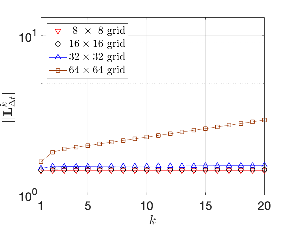
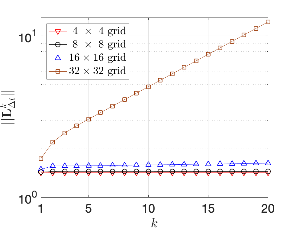
Figure 1: Two-dimensional PDE (37). Operator norm of ${\bf L}^{k}_{\Delta t}$ (see Eq. (38)) versus $k$ for two conditionally stable schemes, namely the second-order centered finite-differences and the Fourier pseudo-spectral collocation schemes on a grid with $n\times n$ evenly-spaced points in $[0,2\pi]^{2}$, with $n=4,8,16,32,64$. It is seen that that the Fourier pseudo-spectral method is less stable than the finite-difference method, in agreement with well-known results [25]. Here we set $\Delta t=0.0025$.

            Full-rank solution                              Low-rank solution

$t=1.2$

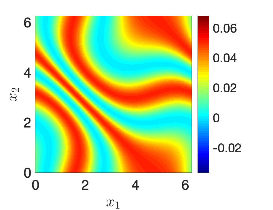
$t=2.5$

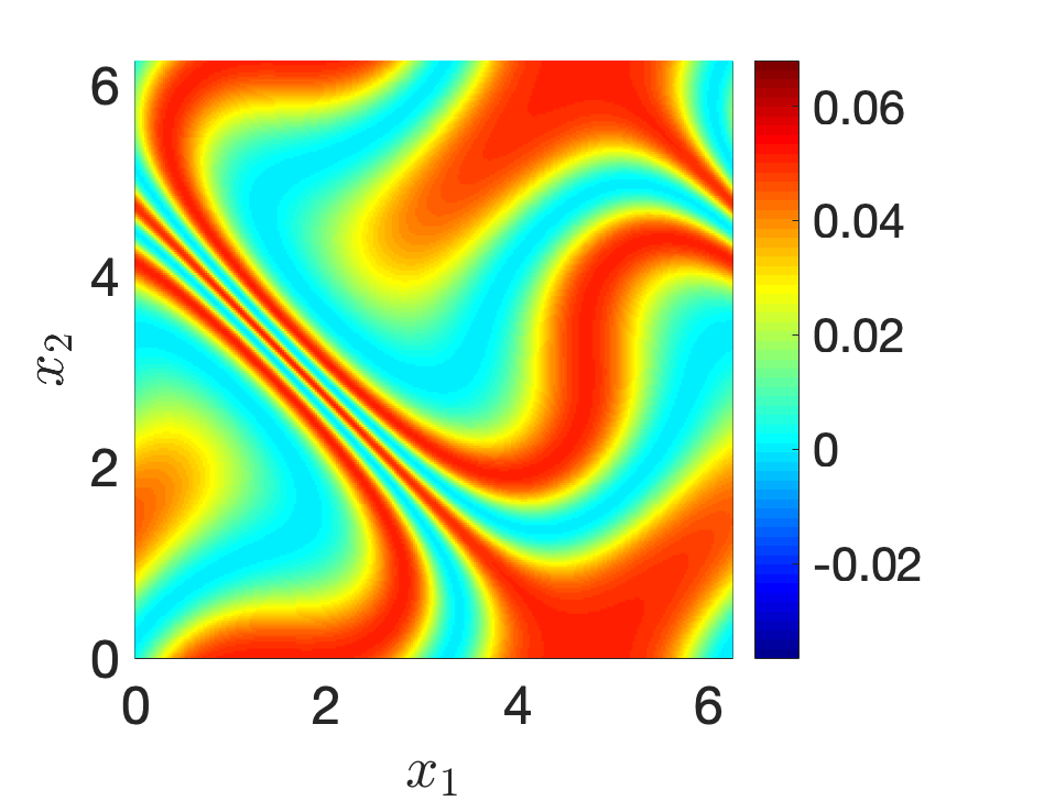
$t=3.8$

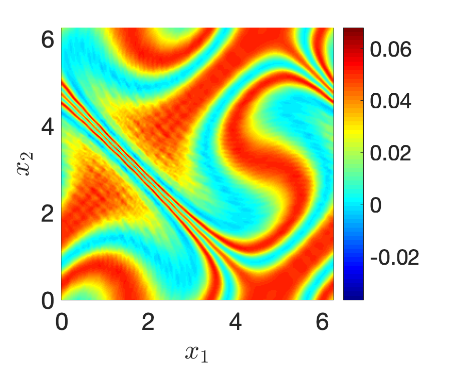
$t=5.0$

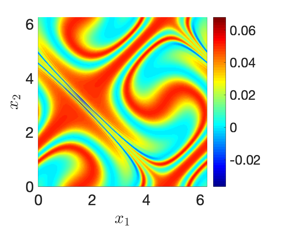
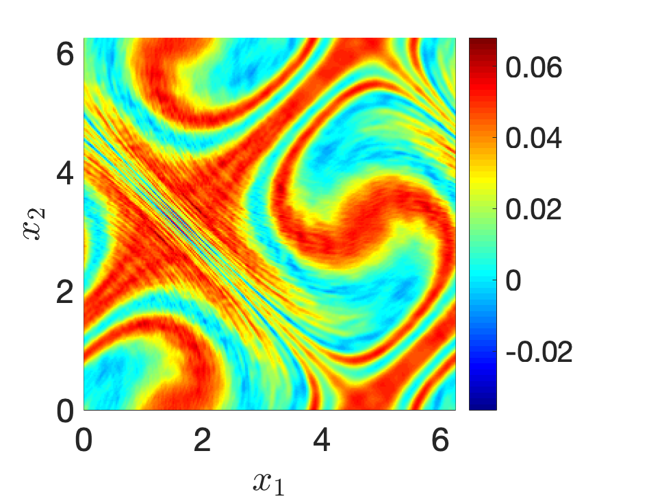
Figure 2: Numerical solution of the PDE (37) using a Fourier pseudo-spectral method on a grid with $256\times 256$ nodes. The initial condition is chosen as $u_{0}(x_{1},x_{2})=\sin^{2}(x_{1}+x_{2})/(2\pi^{2})$. Shown are the full-rank solution (left) and the low-rank tensor solution (right) we obtained by limiting the maximum rank to 64. It is seen that the two solutions are slightly different at $t=3.8$ and $t=5$, but stability is maintained as proven in Theorem 3.1.

In figure 2 we plot the numerical solution of (37) we obtained with an accurate Fourier spectral method. The initial condition is chosen as $u_{0}(x_{1},x_{2})=\sin^{2}(x_{1}+x_{2})/(2\pi^{2})$. It is seen that the low-rank tensor solution obtaining by capping the maximum rank to 64 slightly differs from the full rank solution at $t=3.8$ and $t=5$. However, but stability is maintained as proven in Theorem 3.1. In figure 3 we show that the solution rank grows in time. Such growth is determined by the fact that that solution to the hyperbolic problem (37) becomes harder to resolve as time increases (see figure 2). In particular, in figure 3 we see that just before applying the truncation operator, the rank of the iterate appears to grow at a similar rate to the tensor scheme with no truncation.

Figure 3: Tensor rank of the numerical solution to the PDE (37) versus time. The spatial derivatives are discretized using a Fourier pseudo-spectral method on a grid with $256\times 256$ nodes. Hence the maximum rank of the solution tensor is $256$. The rank-limited solution has maximum rank set to 64. Note that just before applying the truncation operator in a rank-limited scheme, the rank of the iterate appears to grow at a similar rate to the scheme with no truncation. The inaccuracies of the rank-truncated solutions shown in figure 2 at $t=3.8$ and $t=5$ are due to the fact that the solution rank is much larger than 64 at such times (compare red and blue curves).

5.2 Six-dimensional parabolic PDE

We now demonstrate a higher dimensional example which is both highly diffusive and very well approximated by a low-rank numerical solution tensor. To this end, we consider the Fokker-Planck equation (36) with $d=6$. For our numerical demonstration, we consider the following drift and diffusion coefficients

$${\bf f}({\bf x})=\begin{bmatrix}\cos(x_{2})&\sin(x_{3})&\cos(2x_{4})&\sin(2x_{5})&\cos(3x_{6})&\sin(3x_{1})\end{bmatrix}^{T}+6\begin{bmatrix}1&1&1&1&1&1\end{bmatrix}^{T},$$

$${\bf\Gamma}({\bf x})=\begin{bmatrix}5\cos^{2}(x_{6})&\sin(x_{1})&\cos(x_{2})&\sin(x_{3})&\cos(x_{4})&\sin(x_{5})\\ \sin(x_{1})&5\cos^{2}(3x_{3})&\sin(5x_{2})&\cos(2x_{1})&\sin(4x_{6})&\cos(x_{1})\\ \cos(x_{2})&\sin(5x_{2})&5\cos^{2}(3x_{5})&\sin(2x_{3})&\cos(6x_{2})&\sin(x_{6})\\ \sin(x_{3})&\cos(2x_{1})&\sin(2x_{3})&5\cos^{2}(x_{3})&\sin(x_{1})&\cos(4x_{4})\\ \cos(x_{4})&\sin(4x_{6})&\cos(6x_{2})&\sin(x_{1})&5\cos^{2}(5x_{5})&\sin(x_{6})\\ \sin(x_{5})&\cos(x_{1})&\sin(x_{6})&\cos(4x_{4})&\sin(x_{6})&5\cos^{2}(7x_{6})\end{bmatrix}+6{\bf I}.$$

The matrix of drift coefficients was chosen to encourage mixing between different variables and the diffusion coefficients were chosen so that the symmetric matrix is diagonally dominant. Therefore, $\bf\Gamma$ will always be positive definite ensuring that (36) is a bounded diffusion problem. We discretize (36) in space using the Fourier pseudo-spectral collocation method as in 5.1. Specifically, we construct an evenly-spaced grid in $[0,2\pi]^{6}$ with $31$ points in each variable. In principle this yields $31^{6}$ degrees of freedom, which require $110$ MB (Mega Bytes) of storage if a tensor product representation in double precision floating point arithmetic is utilized. However, if we employ a rank $r$ hierarchical Tucker tensor format the memory footprint is reduced to $[r(31\times 6)+4r^{3}+r^{2}]/8$ Bytes. For instance, a rank 40 hierarchical Tucker tensor format in 6 dimensions on a grid with 31 points in each variable requires only $33$ kB (kilo Bytes) of storage. By using the identity $\partial^{2}/\partial x_{k}\partial x_{q}=\partial^{2}/\partial x_{q}\partial x_{k}$, we see that we can just apply the strict upper triangle part of $\bf\Gamma$ once and then double the result. The matrix $\bf G$ at right-hand side of 2 in this case has a rather involved expression and therefore it is not reported here. We supplement (36) with the initial condition in the initial condition

$$u(0,{\bf x})=\frac{1}{\pi^{6}}\prod_{j=1}^{6}\sin(x_{j})^{2}.$$ (40)

Note that (40) is positive and it integrates to one over the hyper-cube $[0,2\pi]^{6}$, i.e., it is a probability density function. In figure 4 we plot the temporal evolution of the marginal PDF

$$u(t,x_{1})=\int_{[0,2\pi]^{5}}u(t,{\bf x})dx_{2}\cdots dx_{6}$$ (41)

It is seen that the PDE (36) is highly diffusive and it yields a solution that can well approximated by a low-rank hierarchical Tucker tensor format.

Max rank 1                                                     Max rank 5

Figure 4: Six-dimensional Fokker-Plank equation (36). Temporal snapshots of the marginal PDF $u(t,x_{1})$. It is seen that the system is highly diffusive and it yields a solution that can well approximated by a low-rank hierarchical Tucker tensor format.

In figure 5 we provide a numerical verification of our Lemma 3.1. To this end, we plot the ratio $\tau_{r}(t)=||{\mathfrak{T}}_{r}({\bf u})||_{2}/||{\bf u}||_{2}$ versus time, and verify that is always smaller than one for any choice of rank. Note that both $\tau_{1}(t)$ and $\tau_{5}(t)$ are very close to 1, which explains why the two plots in Figure 4 are visually identical.

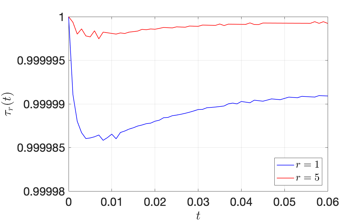
Figure 5: In Lemma 3.1, we proved that the truncation operator ${\mathfrak{T}}_{r}$ satisfies the inequality $||{\mathfrak{T}}_{r}({\bf u})||_{2}\leq||{\bf u}||_{2}$. In this figure we plot of the ratio $\tau_{r}(t)=||{\mathfrak{T}}_{r}({\bf u})||_{2}/||{\bf u}||_{2}$ versus time. We see that setting max rank equal to 5 does in fact give us an extra single digit of accuracy in the nonlinear rank projection. However,$\tau_{1}(t)$ and $\tau_{5}(t)$ are very close to 1, which explains why the two plots in Figure 4 are visually identical.

In our simulations we found that the hierarchical ranks of the HT tensor solution do not grow monotonically as in the two-dimensional advection problem (see figure 3). Instead, they reach a peak very quickly in time. This is because the solution is well approximated by a rank one tensor (see figure 5).

6 Summary

In this paper we studied stability of linear multistep methods (LMM) applied to low-rank tensor discretizations of high-dimensional linear PDEs. In particular, we analyzed the properties of the truncation operator the context of iterated maps and proved boundedness for a wide range of tensor formats. This result allowed us to conclude that LMM is stable on low-rank tensor manifolds provided that it is stable on the full-rank tensor solution. We also showed that PDE solvers with explicit time-stepping may be subject to severe time-step restriction dependent on the dimension of the problem, e.g., on the number of independent spacial variables. We provided demonstrative examples of truncated linear multistep tensor methods applied to variable coefficients linear hyperbolic and parabolic PDEs. Further extensions of the analysis we developed in this paper rely on geometric integration methods. In particular, it was recently shown by Uschmajew and Vandereycken [48] that the hierarchical Tucker tensor manifold with fixed ranks is smooth. This opens the possibility to develop rank-constrained geometric integrators [21] that preserve the structure of the manifold (see, e.g., [34, 28]).

Acknowledgements This research was supported by the U.S. Army Research Office grant W911NF1810309.

Appendix A Brief review of tensor algebra

We regard tensors [29] as elements of $\mathbb{R}^{n_{1}\times\cdots\times n_{d}}$ . Tensors are represented as multidimensional arrays and regarded as being multidimensional arrays to the same extent that linear operators or bi-linear maps may be regarded as matrices, i.e., up to a change in basis. A particular entry in a tensor ${\bf A}$ is denoted by brackets as ${\bf A}[i_{1},\dots,i_{d}]$ where $[i_{1},\dots,i_{d}]\in{\cal I}$ is an array of integers called a multi-index. The set $\cal I$ of all multi-indexes is called an index set. The tensor product is represented by the symbol $\otimes$ and computed for ${\bf A}\in\mathbb{R}^{\mathcal{I}}$, ${\bf B}\in\mathbb{R}^{\mathcal{J}}$ using the definition

$$({\bf A}\otimes{\bf B})[{i},{j}]={\bf A}[{i}\ ]{\bf B}[{j}]\quad\forall{i}\in\mathcal{I},\quad\forall{j}\in\mathcal{J}$$

Both Kronecker and tensor products result in the same array storage in column major format. Their difference only lies in what index lengths are specified, i.e., $\mathbb{R}^{n_{1}\cdot n_{1}}\simeq\mathbb{R}^{n_{1}\times n_{1}}$ within the computer when storing an element as an array.

Matricization of a tensor

A matricization is specific type of permutation on the components of ${\bf A}\in\mathbb{R}^{\mathcal{I}}$ and its indexes such that the resulting tensor is a 2-dimensional array [19], i.e. a matrix. Specifically, let $\cal D$ be an index set, $\rho\subseteq{\cal D}$ be an ordered subset which will define the rows, $\kappa={\cal D}-\rho$ be an ordered subset of all the numbers not in $\rho$, ${\bm{\sigma}}_{\rho}$ be the permutation on sets of size $d$ defined by

$$\bm{\sigma}_{\rho}(1,\dots,d)=(\rho_{1},\dots,\rho_{r},\kappa_{1},\dots,\kappa_{c})$$

where $r+c=d$ are the numbers of row indexes and column indexes, respectively. The $\rho$ mode matricization of $\bf A$ is defined by

$${\bf A}^{(\rho)}[{\rho},{\kappa}]={\bf A}[{i}],\qquad\text{where}\qquad[\rho,\kappa]=\bm{\sigma}_{\rho}(i)\quad\forall{i}\in\mathcal{I}\quad\text{(index set)}.$$

Here $\rho,\kappa$ dermine the row and column of a matrix given by applying a row or column major ordering scheme to the multi-indexes. Applying the inverse of the aforementioned permutation defines a de-matricization, i.e., a transformation back to a tensor. An important case of matricization is the vectorization which corresponds to listing all the entries of $\bf A$ in a single column vector.

$\rho$-mode product

Let ${\bf A}\in\mathbb{R}^{\mathcal{I}}$. Let ${\bf A}^{(\rho)}$ be a matricization of ${\bf A}$ with $R$ rows. Let ${\bf L}\in\mathbb{R}^{M\times R}$ be a matrix. The $\rho$-mode product between ${\bf L}$ and ${\bf A}$, denoted as ${\bf L}\circ_{\rho}{\bf A}$, is defined [16] as the tensor satisfying

$$({\bf L}\circ_{\rho}{\bf A})^{(\rho)}={\bf L}{\bf A}^{(\rho)}$$

This is the action of multiplying into the $\rho$ index or indexes and then summing. The result of the multiplication is achieved by applying the de-matricization permutation. Also note that if $\otimes$ denotes the Kronecker product, then

$${\bf L}\circ_{\lambda}(R\circ_{\rho}{\bf A})\simeq(R\otimes L){\bf A}^{(\lambda\ \cup\ \rho)}$$

so long as $\lambda\ \cap\ \rho$ is empty. Here, $\simeq$ means “up to matricization permutation”. This property is used in Algorithm 941 [30] to compute $\rho$-mode products.

Appendix B Hierarchical Tucker tensor format

The Hierarchical Tucker (HT) tensor format is a decomposition of a tensor obtained by recursively splitting a tensor space into products of pairs of spaces along a binary tree [16]. It was originally introduced by Hackbush and Kühn in [20] to mitigate the curse of dimensionality and storage requirements in the numerical representation of the solution to high-dimensional problems Hereafter we give a brief overview of the HT tensor format. The interested reader is referred to [16, 17, 19, 30]

Dimension Tree

A dimension tree $\mathcal{T}_{d}$ with $d\in\mathbb{N}$ is a tree with an array of integers associated with each node. The root node is defined as the node with the array $[1,\dots,d]$. If $t\in\mathcal{T}_{d}$ is a node on the dimension tree, then the children of $t$ must by definition have arrays which can be concatencated to form the array at $t$. If a tree node has an array with more than one element, it must have children. A node with a singleton array is called a leaf. If a node is not a leaf and not the root, it is called interior. Our definition of dimension tree a slight modification of the definition given in [16, 48, 44]. In particular, we allow for non-binary dimension trees such as that of the Tucker format [19, 16], which looks like a star network topology if the definition above is applied. Of course, a dimension tree is binary if each non-leaf node has two children called “left” and “right”. This can always be accomplished by bisecting the array at a given node. If the array has an odd number of elements, give the left child one more than the right. The HT tensor format corresponds to a binary dimension tree with a matrix (2-tensor) at its root, 3-tensors at the interior nodes, and matrices at the leaves. The 3-tensors are called transfer tensors. If the columns of a leaf matrix are a independent, said matrix is called a leaf frame.

Hierarchical size of a dimension tree

Let $\mathcal{T}_{d}$ be a dimension tree. A hierarchical size associated with $\mathcal{T}_{d}$ is a mapping from the nodes to the natural numbers $\mathbb{N}$. We denote the size at node $t\in\mathcal{T}_{d}$ by $r_{t}$. The definition of hierarchical size is meant to express number of entries stored for each multidimensional array. It corresponds to a specific notion of rank of certain matricizations when finding an estimate of a particular ${\bf A}\in{\mathbb{R}}^{\cal I}$ given a dimension tree. Greater detail is given in [16].

Memory storage format of an HT tensor

Let $\mathcal{I}=\mathcal{I}_{1}\times\dots\times\mathcal{I}_{d}$ be an index set with dimension $d$ and let $N_{\mu}=\max(\mathcal{I}_{\mu})$. Let $\mathcal{T}_{d}$ be a binary dimension tree with hierarchical sizes $r_{t}$. Let $\rho(t)$ denote the right child of $t$ and let $\lambda(t)$ denote the left child. The sizes of the tensors on $\mathcal{T}_{d}$ in the HT format are:

1. At the root node, $\mathcal{D}=\{1,\dots,d\}$, the matrix is denoted by ${\bf B}_{\mathcal{D}}$ and its size is $r_{\lambda(\mathcal{D})}\times r_{\rho(\mathcal{D})}$. We think of ${\bf B}_{\mathcal{D}}$ as being a bilinear form from $\mathbb{R}^{r_{\lambda(\mathcal{D})}}\times\mathbb{R}^{r_{\rho(\mathcal{D})}}$ to $\mathbb{R}$.

2. In the interior nodes, $t\in\mathcal{T}_{d}$, the transfer tensors are written as ${\bf B}_{t}$ and their sizes are $r_{\lambda(t)}\times r_{\rho(t)}\times r_{t}$. We think of ${\bf B}_{t}$ as a bilinear map from $\mathbb{R}^{r_{\lambda(t)}}\times\mathbb{R}^{r_{\rho(t)}}$ to $\mathbb{R}^{r_{t}}$.

3. At the leaves, $\{\mu\}\in\mathcal{T}_{d}$, the matrices are written as $U_{\mu}$ and their sizes are $N_{\mu}\times r_{\{\mu\}}$.

Note that the hierarchical sizes are not necessarily ranks of any of the tensors defined here. Further detail regarding the multilinear algebra of the HT format, including change of basis rules, is described in [48].

Hierarchical rank

Let ${\bf A}\in\mathbb{R}^{\cal I}$ be a tensor corresponding to the dimension tree ${\cal T}_{d}$. The hierarchical rank of ${\bf A}$ is the set of hierarchical sizes defined by $r_{t}=\text{rank}({\bf A}^{(t)})$ for every non-root $t\in{\cal T}_{d}$. For the root, we say the hierarchical rank $r_{t_{root}}=1$ since the matrix there can be seen as a $r_{\lambda}\times r_{\rho}\times 1$ tensor. It is shown in [16] that one can always express a tensor in the HT format using hierarchical sizes equal to the hierarchical ranks of $\bf A$.

Hierarchical truncation

Hierarchical truncation is a generalization of the notion of low-rank SVD-base matrix approximation. This operation is one of the core topics of low-rank tensor approximations [16]. Let ${\bf A}\in\mathbb{R}^{\cal I}$ be a tensor corresponding to the dimension tree ${\cal T}_{d}$, and let ${\cal T}_{d}^{l}$ denote all nodes which are in layer $l$ of the tree, i.e., the number of branch traversals it takes to reach the root. The truncation of $\bf A$ is defined as

$${\mathfrak{T}}_{r}({\bf A}) =\prod_{t\in{\cal T}_{d}^{p}}{\bf P}_{t}\cdots\prod_{t\in{\cal T}_{d}^{1}}{\bf P}_{t}{\bf A}$$

where every ${\bf P}_{t}$ is an orthogonal projection formed using $t$-mode matricizations of $\bf A$. If $\bf A$ is in the HT format, then the resulting truncated tensor may also be expressed in the HT format with hierarchical sizes defined by the matrix ranks of all ${\bf P}_{t}$.

B.1 Parallel implementation

Our complete implementation of the HTucker format in parallel is found in [42]. Each tree node is associated with a different compute node in a manner similar to [17]. Each processor also stores integers to indicate if it is, root, leaf, or interior as well as what its parent/children are. All nodes the Hierarchical Tucker tensor are stored as C++ objects which are instantiated in parallel. Each instance of an HTucker node object communicates with the other nodes on the tree through the Open MPI message passing library. Matrices and tensors are passed through the use of a memory format message encoded in long integers followed by the components of the array passed as double precision floating point numbers. Coding with the library in a driver file largely behaves the same as coding in serial, with memory handled by the package in parallel. Computation on each node is split into cases, where a core is told what to do based on if it is root, interior, or a leaf. This allows for many algorithms to be implemented easily in HTucker format, since tree traversal algorithms can be avoided by simply telling the cores to behave in one of three cases.

References

- [1] M. Bachmayr, R. Schneider, and A. Uschmajew. Tensor networks and hierarchical tensors for the solution of high-dimensional partial differential equations. Foundations of Computational Mathematics, 16(6), 2016.
- [2] J. Baldeaux and M. Gnewuch. Optimal randomized multilevel algorithms for infinite-dimensional integration on function spaces with ANOVA-type decomposition. SIAM J. Numer. Anal., 52(3):1128–1155, 2014.
- [3] V. Barthelmann, E. Novak, and K. Ritter. High dimensional polynomial interpolation on sparse grids. Advances in Computational Mechanics, 12:273–288, 2000.
- [4] C. Beck, W. E, and A. Jentzen. Machine learning approximation algorithms for high-dimensional fully nonlinear partial differential equations and second-order backward stochastic differential equations. J. Nonlinear Sci., 2019.
- [5] R. E. Bellman. Dynamic programming. Princeton University Press, 1957.
- [6] A. M. P. Boelens, D. Venturi, and D. M. Tartakovsky. Parallel tensor methods for high-dimensional linear PDEs. J. Comput. Phys., 375:519–539, 2018.
- [7] H. J. Bungartz and M. Griebel. Sparse grids. Acta Numerica, 13:147–269, 2004.
- [8] Y. Cao, Z. Chen, and M. Gunzbuger. ANOVA expansions and efficient sampling methods for parameter dependent nonlinear PDEs. Int. J. Numer. Anal. Model., 6:256–273, 2009.
- [9] R. Carmona and F. Delarue. Probabilistic theory of mean field games with applications II. Springer, 2018.
- [10] F. Chinesta, R. Keunings, and A. Leygue. The Proper generalized decomposition for advanced numerical simulations. Springer, 2014.
- [11] A. Chkifa, A. Cohen, and C. Schwab. High-dimensional adaptive sparse polynomial interpolation and applications to parametric PDEs. Found. Comput. Math., 14:601–633, 2014.
- [12] V. de Silva and L.-H. Lim. Tensor rank and ill-posedness of the best low-rank approximation problem. SIAM J. Matrix Anal. Appl., 30:1084–1127, 2008.
- [13] A. Dektor and D. Venturi. Dynamically orthogonal tensor methods for high-dimensional nonlinear pdes. ArXiv:1907.05924, pages 1–39, 2019.
- [14] A. Etter. Parallel ALS algorithm for solving linear systems in the hierarchical Tucker representation. SIAM J. Sci. Comput., 38(4):A2585–A2609, 2016.
- [15] J. Foo and G. E. Karniadakis. Multi-element probabilistic collocation method in high dimensions. J. Comput. Phys., 229:1536–1557, 2010.
- [16] L. Grasedyck. Hierarchical singular value decomposition of tensors. SIAM Journal on Matrix Analysis and Applications, 31(4):2029–2054, 2010.
- [17] L. Grasedyck and C. Löbbert. Distributed hierarchical SVD in the hierarchical Tucker format. Numer. Linear Algebra Appl., 25(6):e2174, 2018.
- [18] W. Hackbusch. Tensor spaces and numerical tensor calculus. Springer, 2012.
- [19] W. Hackbusch. Tensor Spaces and Numerical Tensor Calculus. Springer Berlin Heidelberg, 2012.
- [20] W. Hackbusch and S. Kühn. A new scheme for the tensor representation. J. Fourier Anal. Appl., 15(5):706–722, 2009.
- [21] E. Hairer, C. Lubich, and G. Wanner. Geometric numerical integration: structure-preserving algorithms for ordinary differential equations. Springer, 2006.
- [22] E. Hairer, S. P. Nørsett, and G. Wanner. Solving ordinary differential equations. 1, Nonstiff problems. Springer Verlag, 1991.
- [23] G. Heidel and V. Schulz. A Riemannian trust-region method for low-rank tensor completion. Numerical Linear Algebra with Applications, 25(6):e2175, 2018.
- [24] J. S. Hesthaven, S. Gottlieb, and D. Gottlieb. Spectral methods for time-dependent problems. Cambridge University Press, 2007.
- [25] J. S. Hesthaven, S. Gottlieb, and D. Gottlieb. Spectral methods for time-dependent problems. Cambridge University Press, 2007.
- [26] L. Karlsson, D. Kressner, and A. Uschmajew. Parallel algorithms for tensor completion in the CP format. Parallel compting, 57:222–234, 2016.
- [27] B. N. Khoromskij. Tensor numerical methods for multidimensional PDEs: theoretical analysis and initial applications. In CEMRACS 2013–modelling and simulation of complex systems: stochastic and deterministic approaches, volume 48 of ESAIM Proc. Surveys, pages 1–28. EDP Sci., Les Ulis, 2015.
- [28] O. Koch and C. Lubich. Dynamical tensor approximation. SIAM J. Matrix Anal. Appl., 31(5):2360–2375, 2010.
- [29] T. Kolda and B. W. Bader. Tensor decompositions and applications. SIREV, 51:455–500, 2009.
- [30] D. Kressner and C. Tobler. Algorithm 941: htucker – a Matlab toolbox for tensors in hierarchical Tucker format. ACM Transactions on Mathematical Software, 40(3):1–22, 2014.
- [31] L. D. Lathauwer, B. D. Moor, and J. Vandewalle. A multilinear singular value decomposition. SIAM J. Matrix Anal. Appl., 21(4):1253–1278, 2000.
- [32] P. Lax and R. D. Richtmyer. Survery of the stability of linear finite difference equations. Communications on pure and applied mathematics, 9:267–293, 1956.
- [33] G. Li and H. Rabitz. Regularized random-sampling high dimensional model representation (RS-HDMR). Journal of Mathematical Chemistry, 43(3):1207–1232, 2008.
- [34] C. Lubich, B. Vandereycken, and A. Walach. Time integration of rank-constrained Tucker tensors. SIAM J. Numer. Anal., 56(3):1273–1290, 2018.
- [35] A. Narayan and J. Jakeman. Adaptive Leja sparse grid constructions for stochastic collocation and high-dimensional approximation. SIAM J. Sci. Comput., 36(6):A2952–A2983, 2014.
- [36] I. V. Oseledets. Tensor-train decomposition. SIAM J. Sci. Comput., 33(5):2295––2317, 2011.
- [37] M. Raissi and G. E. Karniadakis. Hidden physics models: Machine learning of nonlinear partial differential equations. J. Comput. Phys., 357:125–141, 2018.
- [38] M. Raissi, P. Perdikaris, and G. E. Karniadakis. Physics-informed neural networks: A deep learning framework for solving forward and inverse problems involving nonlinear partial differential equations. J. Comput. Phys., 378:606–707, 2019.
- [39] S. C. Reddy and L. N. Trefethen. Lax stability of fully discrete spectral methods via stability region and pseudo-eigenvalues. Computer methods in applied mechanics and engineering, 80:147–164, 1990.
- [40] S. C. Reddy and L. N. Trefethen. Stability of the method of lines. Numer. Math., 62:235–267, 1992.
- [41] H. Risken. The Fokker-Planck equation: methods of solution and applications. Springer-Verlag, second edition, 1989. Mathematics in science and engineering, vol. 60.
- [42] A. Rodgers. htucker-mpi. https://github.com/akrodger/htucker-mpi, 2019.
- [43] T. Rohwedder and A. Uschmajew. On local convergence of alternating schemes for optimization of convex problems in the tensor train format. SIAM J. Numer. Anal., 51(2):1134–1162, 2013.
- [44] C. Da Silva and F. J. Herrmann. Optimization on the hierarchical Tucker manifold – Applications to tensor completion. Linear Algebra and its Applications, 481:131–173, 2015.
- [45] S. T. Smith. Optimization techniques on Riemannian manifolds. Fields Institute Communications, 3:113–136, 1994.
- [46] J. C. Strikwerda. Finite difference schemes and partial differential equations. SIAM, second edition, 2004.
- [47] S. Torquato. Random heterogeneous materials, microstructure and macroscopic properties. Springer, 2002.
- [48] A. Uschmajew and B. Vandereycken. The geometry of algorithms using hierarchical tensors. Linear Algebra Appl., 439(1):133–166, 2013.
- [49] B. Vandereycken. Low-rank matrix completion by Riemannian optimization. SIAM J. Optim., 23(2):1214–1236, 2013.
- [50] D. Venturi. The numerical approximation of nonlinear functionals and functional differential equations. Physics Reports, 732:1–102, 2018.
- [51] D. Venturi and G. E. Karniadakis. Convolutionless Nakajima-Zwanzig equations for stochastic analysis in nonlinear dynamical systems. Proc. R. Soc. A, 470(2166):1–20, 2014.
- [52] D. Venturi, T. P. Sapsis, H. Cho, and G. E. Karniadakis. A computable evolution equation for the joint response-excitation probability density function of stochastic dynamical systems. Proc. R. Soc. A, 468(2139):759–783, 2012.
- [53] R. Le Veque. Finite Difference Methods for Ordinary and Partial Differential Equations. Society for Industrial and Applied Mathematics, 2007.
- [54] C. Villani. Optimal transport: old and new. Springer, 2009.
- [55] G. Wanner and E. Hairer. Solving ordinary differential equations II. Springer, 1996.
- [56] Y. Zhu, N. Zabaras, P.-S. Koutsourelakis, and P. Perdikaris. Physics-constrained deep learning for high-dimensional surrogate modeling and uncertainty quantification without labeled data. J. Comput. Phys., 394:56–81, 2019.