SPGNet: Semantic Prediction Guidance for Scene Parsing

Abstract

Multi-scale context module and single-stage encoder-decoder structure are commonly employed for semantic segmentation. Multi-scale context module aggregates feature responses from a large spatial extent, while the single-stage encoder-decoder structure encodes the high-level semantic information in the encoder path and recovers the boundary information in the decoder path. In contrast, multi-stage encoder-decoder networks have been widely used in human pose estimation and shown superior performance than their single-stage counterpart. However, few efforts have been attempted to bring this effective design to semantic segmentation. In this work, we propose a Semantic Prediction Guidance (SPG) module which learns to re-weight the local features through the guidance from pixel-wise semantic prediction. We find that by carefully re-weighting features across stages, a two-stage encoder-decoder network coupled with our proposed SPG module can significantly outperform its one-stage counterpart with similar parameters and computations. Finally, we report experimental results on the semantic segmentation benchmark Cityscapes, in which our SPGNet attains 81.1% on the test set using only ‘fine’ annotations.

1 Introduction

(a) Squeeze-and-Excite [25].

(b) Gather-and-Excite [24].

(c) Our proposed Supervise-and-Excite.

Figure 1: Three different frameworks for re-weighting local features. Dotted square areas with lighter color in (a) and (b) denote average pooling operations.

Semantic segmentation [21], as a step towards scene understanding [56, 31, 69, 55], is a challenging problem in computer vision. It refers to the task of assigning semantic labels, such as person and sky, to every pixel within an image. Recently, Deep Convolutional Neural Networks (DCNNs) [32, 30] have significantly improved the performance of semantic segmentation systems.

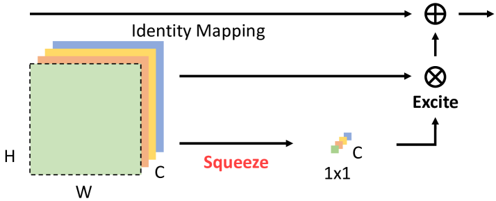
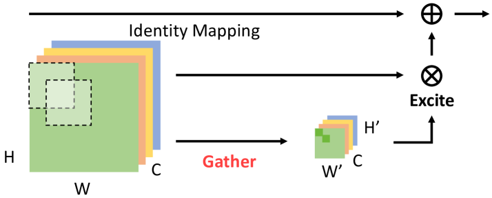
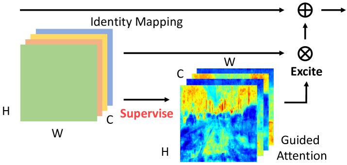
In particular, DCNNs, deployed in a fully convolutional manner [50, 40], have attained remarkable results on several semantic segmentation benchmarks [16, 14, 77]. We observe two key design components shared among state-of-the-art semantic segmentation systems. First, multi-scale context module, exploiting the large spatial information, enriches the local features. Typical examples include DeepLab [7] which adopts several parallel atrous convolutions [22, 44] with different rates and PSPNet [75] which performs pooling operations at different grid scales. Recently, SENets [25] and GENets [24] employ the ‘squeeze-and-excite’ (Figure 1 (a)) or more general ‘gather-and-excite’ framework (Figure 1 (b)) and obtain remarkable results on image classification task. Motivated by this, we propose a simple yet effective attention module, called Semantic Prediction Guidance (SPG), which learns to re-weight the local feature map values via the guidance from pixel-wise semantic prediction. Unlike the ‘gather-and-excite’ module [25, 24] (where context information is gathered from a large spatial extent and local features are excited accordingly), our SPG module adopts the ‘supervise-and-excite’ framework (Figure 1 (c)). Specifically, we inject the semantic supervision to the feature maps followed by a simple $1\times 1$ convolution with sigmoid activation function (i.e., ‘supervise’ step). The resulting feature maps, called “Guided Attention”, are used as a guidance to re-weight the other transformed feature maps correspondingly (i.e., ‘excite’ step). We further add an ‘identity’ mapping in the module, similar to the residual block [20]. Additionally, our learned “Guided Attention” allows us to visually explain the “re-weighting” mechanism in our SPG module.

Another important design component is the encoder-decoder structure, where high-level semantic information is captured in the encoder path while the detailed low-level boundary information is recovered in the decoder path. The systems [43, 48, 3, 36, 46, 45, 1, 74, 65, 11, 62], employing the single-stage encoder-decoder structure (i.e., the encoder-decoder structure is stacked only once), have demonstrated outstanding performance on several semantic segmentation benchmarks. On the other hand, the multi-stage encoder-decoder models [61, 5, 41, 42, 68, 28, 33], also known as stacked hourglass networks [42], refine the keypoint estimation iteratively by propagating information across stages for the task of human pose estimation. Interestingly, we observe that the multi-stage encoder-decoder structure is seldom explored in the context of semantic segmentation, except [19, 51]. In this work, we revisit the multi-stage encoder-decoder networks on the Cityscapes dataset [14]. We find that by carefully selecting features across stages, a two-stage encoder-decoder network coupled with our proposed SPG module can significantly outperform its one-stage counterpart with similar parameters and computations.

On Cityscapes test set [14], our proposed SPGNet outperforms the strong baseline DenseASPP [66] when only exploiting the ‘fine’ annotations. Our overall mIoU is slightly behind the concurrent work DANet [18] but detailed class-wise mIoU reveals that our model is better than DANet in 14 out of 19 semantic classes. Furthermore, our SPGNet requires only $22.7\%$ computation of DANet [18].

To summarize our main contributions:

• We propose a simple yet effective attention module, called SPG, which adopts a ‘supervise-and-excite’ framework.

• We explore multi-stage encoder-decoder networks on semantic segmentation task. Incorporating our proposed SPG module to the multi-stage encoder-decoder networks further improves the performance.

• We demonstrate the effectiveness of our SPGNet on the challenging Cityscapes dataset. Our model outperforms the strong baseline DenseASPP [66], and is better than DANet [18] in 14 out of 19 semantic classes. Our SPGNet strikes a better accuracy/speed trade-off, requiring only $22.7\%$ computation of DANet.

• We provide detailed ablation studies along with the visualization of our learned attention maps. We also discuss the effectiveness of employing multi-stage encoder-decoder networks on semantic segmentation.

Figure 2: The overall structure of SPGNet. Only two stages are shown for simplicity and it can be easily generalized to more stages. (a) Our encoder-decoder design. (b) Upsample module. (c) Cross stage feature aggregation [33]. GAP: global average pooling [39]. Residual Block: same bottleneck module used in ResNet [20]. Upsample: bilinear upsampling by x2. SPG: semantic prediction guidance module.

2 Related Works

Semantic Segmentation: Most state-of-the-art semantic segmentation models are based on FCN [50, 40]. The detailed object boundary information is usually missing due to the pooling or convolutions with striding operations within the network. To alleviate the problem, one could apply the atrous convolution [22, 50, 44, 7] to extract dense feature maps. However, it is computationally expensive to extract output feature maps that are 8 or even 4 times smaller than the input resolution using state-of-the-art network backbones [30, 52, 54, 20]. On the other hand, the encoder-decoder structures [43, 48, 3, 36, 46, 45, 1, 19, 74, 65, 11, 62, 27] capture the context information in the encoder path and recover high resolution features in the decoder path. Additionally, contextual information has also been explored. ParseNet [39] exploits the global context information, while PSPNet [75] uses spatial pyramid pooling at several grid scales. DeepLab [8, 9, 38, 67] uses several parallel atrous convolution with different rates in the Atrous Spatial Pyramid Pooling module, while DPC [6] applies neural architecture search [78] for the context module. Finally, our proposed Semantic Prediction Guidance (SPG) bears a similarity to the Layer Cascade method [34] which treats each pixel differently. Instead of classifying easy pixels in the early stages within the network, our SPG module weights each pixel according to the predictions in the first stage of our stacked network.

Multi-Stage Networks: Multi-stage networks [61, 5, 41, 42, 68, 28, 33, 53, 59] have been widely used and explored in human pose estimation. Multi-stage networks aim to iteratively refine estimation. To maximally utilize the capacity of each stage, CPM [61] and Stacked Hourglass [42] propagate not only features to the next stage, but also remap predicted heatmaps into feature space by a 1x1 convolution and concatenate with feature maps. MSPN [33] further optimizes feature flow across stages by propagating intermediate features of encoder-decoder of previous stage to the next stage. MSPN [33] demonstrates superior performance over single stage counterpart with similar parameters and computations. On the other hand, Stacked Deconvolutional Network [19] uses multiple deconvolution networks for semantic segmentation. However, it only passes features across stages and neglects predictions of every stage. Additionally, Zhou et al. [77] propose a cascade segmentation module. In this work, we find predictions can be served as a special attention to propagate useful features across stages.

Attention Module: Attention mechanism has been widely used recently in multiple computer vision tasks. Chen et al. [10] learn an attention module to merge multi-scale features. Kong and Fowlkes [29] propose a gating module that adaptively selects features pooled with different field sizes. Recently, the self-attention module [57] has been explored by several works [23, 60, 18, 13, 26] for computer vision tasks. In contrast, our proposed SPG module is more similar to the other works that employ the ‘squeeze-and-excite’ or ‘gather-and-excite’ framework. In particular, Squeeze-and-Excitation Networks (SENets) [25] squeeze the features across spatial dimensions to aggregate the information for re-weighting feature channels. Hu et al. [24] generalize SENets with ‘gather-and-excite’ operations where long-range spatial information is gathered to re-weight (or ‘excite’) the local features. Motivated by this, our proposed SPG module employs the ‘supervise-and-excite’ framework, where our local features are guided by the semantic supervision. Additionally, EncNet [72] also adds supervision to their global feature. However, our supervision is pixel-level instead of image-level.

3 Methods

3.1 Overall Architecture

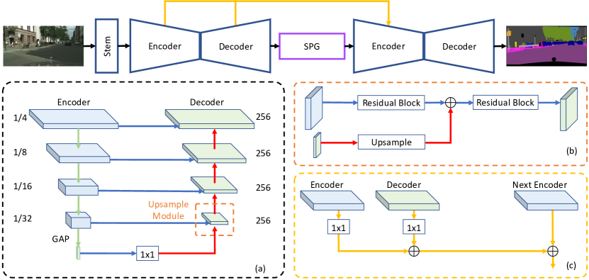
Figure 2 shows our proposed SPGNet, which consists of multiple stages and each stage is based on an encoder-decoder architecture: encoder produces dense feature maps at multiple scales and also an image-level feature vector using global average pooling (GAP). Decoder starts with this feature vector and gradually recovers spatial resolution by combining corresponding encoder feature map using an upsample module, described in Sec 3.3.

Our SPGNet stacks multiple stages, where earlier decoder output is fed into a semantic prediction guidance (SPG) module (detailed in Sec 3.4) to generate input feature for the next stage. In addition, we employ Cross Stage Feature Aggregation [33] to enhance latter stage encoders by taking advantage of earlier stage encoder / decoder features, as shown in Figure 2(c). The decoder output in the final stage is bilinearly upsampled to input image resolution, generating per-pixel semantic prediction results.

The multi-stage design of SPGNet is inspired by Stacked Hourglass [42] for human pose estimation. Our method differs from Stacked Hourglass in 1) we carefully design the encoder-decoder architecture in each stage instead of using a symmetric hourglass network, and 2) latter stage input is generated from SPG module rather than simply passing the features combined with predictions from previous stage.

3.2 Encoder / Decoder Design

Hourglass networks [42] assign equal computation to both encoder and decoder, making it unavailable to use pre-trained weights on ImageNet [15]. In contrast, Feature Pyramid Networks (FPN) [37] use well-designed classification networks for encoder and design a simple decoder consisting of only nearest-neighbor interpolations to upsample decoder feature maps. Our encoder-decoder design principles follow FPN (e.g., all the feature maps in the decoder contain 256 channels), but we employ two more components to make it more efficient and effective. First, we incorporate a global average pooling [39] after the output of encoder to generate the $1\times 1$ image-level features followed by another $1\times 1$ convolution to transform its feature channels to 256. Second, instead of using a single nearest-neighbor interpolation, we design an efficient upsample module, as described in the next section.

3.3 Upsample module

As illustrated in Figure 2(a, b), our decoder adopts upsample module to recover feature map resolution step-by-step. Specifically, each module in the decoder takes two input feature maps, one from encoder and one from previous layer output. The input from encoder is first transformed by a residual block to reduce the dimension to output channel of the decoder. Then, the input from previous layer output is bilinear upsampled and added to the transformed encoder output. Instead of passing this merged feature directly to next upsample module, we further add another residual block to better fuse features from two different sources.

3.4 Semantic Prediction Guidance

Figure 3: Our Semantic Prediction Guidance (SPG) module.

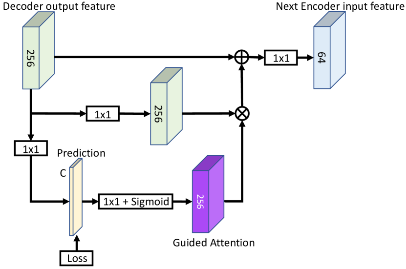
Using contextual information to re-weight feature channels [25, 24] has brought significant improvements to image classification task. This process usually includes a ‘gather’ step which collects information over a large spatial region. In contrast, in our multi-stage encoder-decoder network, the output features generated from each stage already contain information from multiple scales. This inspires us to design a simple yet effective SPG module (Figure 3) which treats the features from earlier stage as ‘gathered’ information. Specifically, the previous stage decoder output feature $x_{d}\in\mathbb{R}^{H\times W\times D}$ is first fed into a $1\times 1$ convolution to produce per-class logits $x_{l}\in\mathbb{R}^{H\times W\times C}$, where $H$ and $W$ are decoder output height and width, $D$ is the number of channels used in the decoder and $C$ is the number of semantic classes in the dataset. We then produce a per-pixel, per-channel Guided Attention mask $m\in\mathbb{R}^{H\times W\times D}$ from $x_{l}$ via a simple $1\times 1$ convolution followed by sigmoid activation. This Guided Attention will be element-wise multiplied to a transformed decoder feature map, generated from $1\times 1$ convolution on top of $x_{d}$, resulting in an attention-augmented feature map. Similar to residual block, this feature map is added back to decoder output feature $x_{d}$, followed by another $1\times 1$ convolution to produce input feature to the next stage encoder. During training, we minimize the loss of last-stage semantic prediction and per-class logits $x_{l}$ in all previous stages.

Our proposed SPG module differs from SENets [25] and GENets [24] on using supervised semantic predictions to guide the ‘excite’ step. We further verified having explicit supervision improves model performance. The benefit of our proposed SPG module are twofold: the ‘gather’ step is implicitly folded into the encoder-decoder architecture, which allows SPG module to be computationally efficient (about $1\%$ increase in FLOPs) and have a small memory footprint ($2.3\%$ higher peak memory usage). Meanwhile, using semantic prediction makes SPG module more explainable. See Section 4.5 for visualization.

4 Experiments

4.1 Dataset

We perform experiments on the Cityscapes dataset [14], which contains 19 classes. There are 5,000 images with high quality annotation (called “fine”), divided into 2,975/500/1,525 images for training, validation and testing. We only use the “fine” annotation in this paper.

4.2 Implementation Details

Networks. We employ ResNet [20] in the encoder module. The “Stem” in Figure 2 consists of a $7\times 7$ convolution with stride $=2$ followed by a $3\times 3$ max pooling with stride $=2$. We replace BatchNorm layers with synchronized Inplace-ABN [49], and adopt bilinear interpolation in all the upsampling operations.

Training settings. We use mini-batch SGD momentum optimizer with batch size 8, initial learning rate 0.01, momentum 0.9 and weight decay 0.0001. Following prior works [39], we use the “poly” learning rate schedule where the learning rate is scaled by $(1-\frac{\text{iter}}{\text{iter}_{\text{max}}})^{0.9}$. For data augmentation, we employ random scale between [0.5, 2.0] with a step size of 0.25, random flip and random crop. We train the model for $80,000$ iterations on “train”set for ablation study. To evaluate our model on the “test” set, we train the model on the concatenation of “train” and “val” set.

4.3 Comparison with State-of-the-Arts

Method	Backbone	mIoU ($\%$)	#Params	#FLOPs†
RefineNet [36]	ResNet-$101$	$73.6$	-	-
DUC-HDC [58]	ResNet-$101$	$77.6$	$65.0$M	$2234.3$B
SAC [73]	ResNet-$101$	$78.1$	-	-
DepthSeg [29]	ResNet-$101$	$78.2$	-	-
PSPNet [75]	ResNet-$101$	$78.4$	$65.7$M	$2117.3$B
BiSeNet [70]	ResNet-$101$	$78.9$	$51.6$M	$429.5$B
DFN [71]	ResNet-$101$	$79.3$	$112.0$M	$2239.6$B
PSANet [76]	ResNet-$101$	$80.1$	-	-
DenseASPP [66]	DenseNet-$161$	$80.6$	$35.4$M	$1240.1$B
DANet [18]	ResNet-$101$	$81.5$	$66.5$M	$2878.9$B
SPGNet (Ours)	$2\times$ ResNet-$50$	$\bf{81.1}$	$59.8$M	$654.8$B

• #FLOPs take all matrix multiplication into account.

Table 1: Comparison to state-of-the-art on Cityscapes test set.

Methods Mean IoU road sidewalk building wall fence pole traffic light traffic sign vegetation terrain sky person rider car truck bus train motorcycle bicycle DenseASPP [66] 80.6 98.7 87.1 93.4 60.7 62.7 65.6 74.6 78.5 93.6 72.5 95.4 86.2 71.9 96.0 78.0 90.3 80.7 69.7 76.8 DANet [18] 81.5 98.6 86.1 93.5 56.1 63.3 69.7 77.3 81.3 93.9 72.9 95.7 87.3 72.9 96.2 76.8 89.4 86.5 72.2 78.2 SPGNet (ours) 81.1 98.8 87.6 93.8 56.5 61.9 71.9 80.0 82.1 94.1 73.5 96.1 88.7 74.9 96.5 67.3 84.8 81.8 71.1 79.4

Table 2: Per-class results on Cityscapes test set. SPGNet outperforms existing top approaches in 13 out of 19 classes.

In Table 1, we report our Cityscape “test” set result. We only use “fine” annotations and thus compare with the other state-of-art models that adopt the same setting in the table. Similar to other models, we use the multi-scale inputs (scales = $\{0.75,1.0,1.25,1.5,1.75,2.0\}$) during inference. We also report the model parameters and computation FLOPs (w.r.t., a single $1024\times 2048$ input size).

Our best SPGNet model variant employs a 2-stage encoder-decoder structures with ResNet-50 as encoder backbone and decoder channels $=256$. Our model outperforms most top-performing approaches on Cityscapes with much less computation. Notably, most state-of-the-art methods are mainly based on systems using atrous convolutions to preserve feature maps resolution, which however requires a large amount of computation (as indicated by #FLOPs in Table 1). On the contrary, our proposed SPGNet, built on top of an efficient encoder-decoder structure, strikes a better trade-off between accuracy and speed.

To be concrete, the computation of our SPGNet is almost half of DenseASPP, the previous published state-of-the-art model using only fine annotations, but our performance is $0.5\%$ mIoU better. We also compare our SPGNet with another concurrent work DANet [18]. Our computation is around $22.7\%$ of DANet with only $0.4$ mIoU degradation.

We further compare per-class results with the top-2 performing approaches in Table 2. Surprisingly, our SPGNet outperforms DenseASPP in 15 out of 19 classes and DANet in 14 out of 19 classes. The main degradation of our overall mIoU comes from the “truck” class which is $10.7$ IoU worse than DenseASPP and $9.5$ IoU worse than DANet. We think it is because there are only few “truck” annotations in Cityscapes and our SPGNet requires supervision for learning the guided attention.

4.4 Ablation Studies

Here, we provide ablation studies on Cityscapes val set.

Effect of SPG module.

#Stage	SPG	Id.	Sup.	mIoU ($\%$)	#Params	#FLOPs
$1$	-	-	-	$74.48$	$11.7$M	$107.6$B
$2$	✗	-	-	$76.31$	$23.9$M	$215.5$B
$2$	✓(sum)	✓	✓	$76.96$	$23.9$M	$218.0$B
$2$	✓(softmax)	✓	✓	$77.17$	$23.9$M	$218.0$B
$2$	✓(sigmoid)	✓	✓	77.67	$23.9$M	$218.0$B
$2$	✓(sigmoid)	✗	✓	$77.24$	$23.9$M	$218.0$B
$2$	✓(sigmoid)	✓	✗	$77.12$	$23.9$M	$218.0$B

Table 3: Cityscapes ablation studies of proposed SPG on validation set. All models use ResNet-18 in encoder. Id.: Adding the identity mapping path in SPG. Sup.: Adding the semantic supervision in SPG. Employing sigmoid activation, identity mapping path, and supervision in our SPG with 2 stages attains the best performance.

We perform ablation studies on the SPG design in Table 3. The baseline is a simple 2-stage encoder-decoder network by directly passing the 1st stage decoder features to the 2nd stage encoder. This baseline model uses the Cross-Stage Feature Aggregation (CSFA) [33] which is slightly better than the case without CSFA by 0.18%. We first verify whether passing semantic prediction together with the decoder features to next stage is helpful. We transform the predictions from the 1st stage decoder output by applying a $1\times 1$ convolution. The sum of the transformed predictions and the 1st stage decoder output is passed to the next stage (denoted as SPG (sum)). It achieves $76.96\%$ mIoU which is $0.65\%$ mIoU better than the baseline. Additionally, our proposed SPG module uses the transformed semantic predictions to ‘excite’ the decoder features. We explore two ways for excitation: one is by applying softmax on the spatial dimension $\text{H}\times\text{W}$ (SPG (softmax)) and the other is using sigmoid (SPG(sigmoid)). The SPG (softmax) scheme improves the baseline by $0.86\%$ mIoU while the SPG (sigmoid) scheme achieves the best mIoU of $77.67\%$ ($1.36\%$ mIoU better than the baseline). Comparing results of SPG (sigmoid) scheme ($77.67\%$ mIoU) with SPG (sum) scheme ($76.96\%$ mIoU), it shows the importance of using ‘Excite’ to re-weight features. Finally, we investigate the effect of adding the identity mapping path and the supervision in SPG module. Dropping the identity mapping path in Figure 3 degrades the performance from $77.67\%$ to $77.24\%$, while removing the supervision on learning the guided attention decreases the performance to $77.12\%$ in which our SPG module degenerates to a special case of ‘gather-and-excite’ (where the features are ‘gathered‘ from the 1st-stage decoder output).

SPG module vs SE/GE module.

Module	Supervise	mIoU ($\%$)
SE [25]	✗	$77.09$
GE [24]	✗	$77.22$
SPG (Ours)	✓	77.67

Table 4: Cityscapes val ablation studies on Supervise-and-Excite. All models use ResNet-18 in encoder. Our proposed Supervise-and-Excite has advantage over Squeeze/Gather-and-Excite.

To demonstrate the gain of SPG module comes from supervision, we compare SPG module with its unsupervised counterpart, i.e. SE [25] and GE [24] modules. Using SE and GE modules achieves 77.09 mIoU and 77.22 mIoU respectively, both results are better than the baseline 76.31 mIoU and using GE is slightly better than SE which is consistent with the findings in [24]. However, they are still worse than using our proposed supervise-and-excite (i.e. SGP with 77.67 mIoU). The additional gain mainly comes from adding supervision in supervise-and-excite.

More stages.

#Stage	mIoU ($\%$)	#Params	#FLOPs
$1$	$74.48$	$11.7$M	$107.6$B
$2$	77.67	$23.9$M	$218.0$B
$3$	$77.66$	$36.2$M	$328.5$B

Table 5: Cityscapes ablation studies on validation set. All models use ResNet-18 in encoder. SPG with 2 stages is the optimal choice.

We experiment the effect of using more stages and the results are shown in Table 5. Similar to the situation in pose estimation that performance gets saturated as the number of stages increases. But in our case the performance saturates very quickly and achieves optimal with 2 stages. It is possible that by carefully balancing the loss weights among stages the performance might be better for models with more than 2 stages. However, for simplicity, we focus on models with only 2 stages in this paper.

Effect of encoder combination.

Encoder combination	mIoU ($\%$)	#Params	#FLOPs
ResNet-$18$ + ResNet-$18$	$77.67$	$23.9$M	$218.0$B
ResNet-$18$ + ResNet-$50$	$78.34$	$38.4$M	$336.0$B
ResNet-$50$ + ResNet-$18$	$78.83$	$38.0$M	$329.9$B
ResNet-$50$ + ResNet-$50$	$79.81$	$55.6$M	$467.6$B

Table 6: Cityscapes val ablation studies of encoder combination (ResNet-18 and ResNet-50). In our two-stage SPGNet, it is effective to employ a deeper backbone in the 1st encoder module.

Our two-stage SPGNet could potentially employ two different backbones in each encoder module. As shown in Table 6, although employing ResNet-$18$+ResNet-$50$ (i.e., ResNet-18 in the 1st encoder and ResNet-50 in the 2nd encoder) and ResNet-$50$+ResNet-$18$ have similar parameters and computation, using deeper model in the first stage outperforms the other one. We think it is crucial to “encode” the features in the early stage with a stronger backbone. Adopting R-$50$+R-$50$ achieves the best performance. For simplicity, we only adopt the same network backbones in all the encoder modules in this paper.

Encoder depth.

Backbone	#Stage	Channel	mIoU ($\%$)	#Params	#FLOPs
ResNet-18	$1$	128	$74.48$	$11.7$M	$107.6$B
ResNet-50	$1$	128	$77.80$	$24.7$M	$212.9$B
ResNet-101	$1$	128	$78.72$	$43.7$M	$371.7$B
ResNet-152	$1$	128	$78.33$	$59.4$M	$530.1$B
ResNet-18	$2$	128	$77.67$	$23.9$M	$218.0$B
ResNet-50	$2$	128	$79.81$	$55.6$M	$467.6$B
ResNet-101	$2$	128	80.04	$93.5$M	$785.3$B

Table 7: Cityscapes val ablation studies on encoder depth. Using deeper encoder in general has better performance.

In Table 7, we study the effect of adopting different backbones in the encoder module(s). We observe that using deeper encoder improves the result and using ResNet-50 in a 2-stage SPGNet achieves a good trade-off between #Params, #FLOPs and performance.

Hard example mining.

Backbone	#Stage	Channel	OHEM	mIoU ($\%$)
ResNet-50	$2$	128	✗	$79.81$
ResNet-50	$2$	128	✓	80.10
ResNet-101	$2$	128	✗	$80.04$
ResNet-101	$2$	128	✓	80.85

Table 8: Cityscapes val ablation studies on On-line Hard Example Mining (OHEM). SPG benefits from OHEM.

We study the effects of on-line hard example (or pixel) mining (OHEM) [63, 4, 67] in Table 8. We apply OHEM to all stages (i.e., the decoder output in each stage) in our SPGNet. As shown in the table, using OHEM consistently improves the performance.

Decoder channels.

Backbone	Channel	mIoU ($\%$)	#Params	#FLOPs
ResNet-50	128	$80.10$	$55.6$M	$467.6$B
ResNet-50	256	80.91	$59.8$M	$654.8$B
ResNet-101	128	$80.85$	$93.5$M	$785.3$B
ResNet-101	256	$80.42$	$97.8$M	$972.4$B

Table 9: Cityscapes val ablation studies on decoder channel. All models are #Stage=2 and use OHEM in training.

We experiment on the effect of decoder channels in Table 9. Employing ResNet-50 as the encoder backbone and decoder channels $=256$ achieves the best validation mIoU.

Flip and multi-scale test. We further add flip and multi-scale test to the best model (ResNet-50 with 2 stages, in Table 9). By adding scales = $\{0.75,1.0,1.25,1.5,1.75,2.0\}$, the performance further improves from 80.91 to 81.86.

Figure 4: Method to visualize guided attention.

Image	Prediction	Car	Person	Building	Pole

Figure 5: Visualization of guided attention for 4 general classes. Guided attention focuses on the boundary of co-occurred objects/things.

Image	Prediction	Person	Rider

Figure 6: Visualization of guided attention for Person/Rider. Guided attention is capable of differentiating semantically similar classes.

Image	Prediction	Truck	Bus	Train

Figure 7: Visualization of guided attention for Truck/Bus/Train. Our failure cases where guided attention confuses among Truck/Bus/Train.

4.5 Visualization of Guided Attention

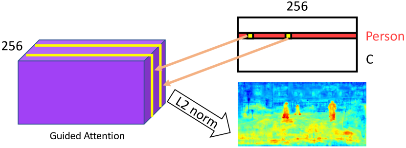
In this section, we visualize the learned Guided Attention in our best model variant (a stack of two encoder-decoder structures with ResNet-50 as encoder backbone). The Guided Attention maps (with 256 channels) is obtained by applying a $1\times 1$ convolution with sigmoid activation to the prediction in the 1st stage decoder output. Therefore, we have a convolution weight matrix with size $C\times 256$ (Figure 4 top-right), where $C$ is the number of semantic classes on the dataset. To visualize the attention for class $c$, we would like to know which channels among the 256 channels in the Guided Attention map that the class $c$ contributes most. Therefore, for class $c$, we extract the corresponding $1\times 256$ convolution weight vector (Figure 4 red row in matrix) from the $C\times 256$ matrix. In the vector, we then select the indexes of the top $15$ largest weights (Figure 4 yellow elements in vector), which is used to index the corresponding channels in the Guided Attention maps (Figure 4 yellow slices from the purple Guided Attention maps), i.e., those channels in the Guided Attention maps have the largest responses for the class $c$. Then, we visualize the attention by taking $l_{2}$ norm of the selected channels.

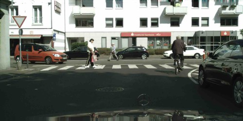
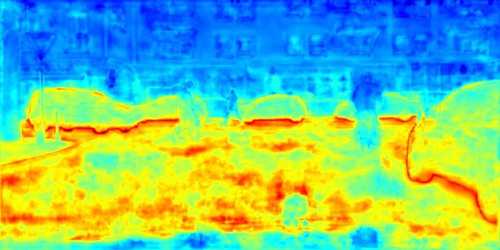
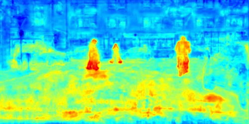
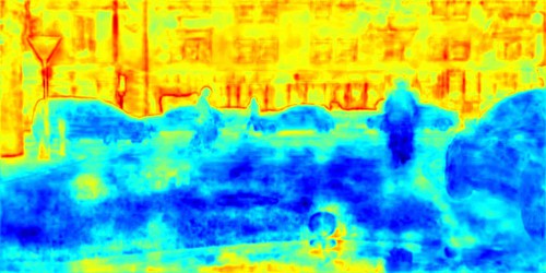
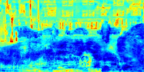
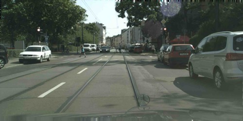
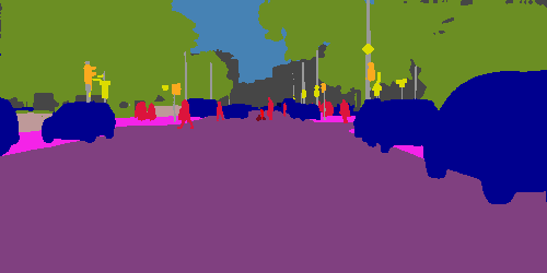
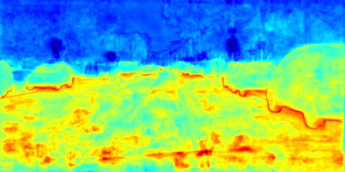
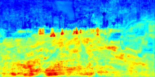
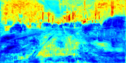
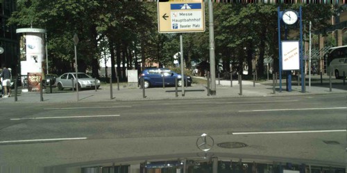
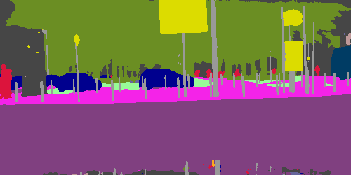
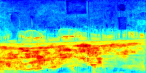
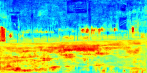
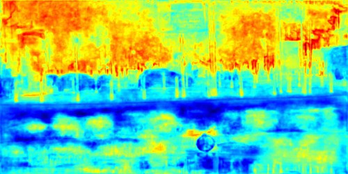
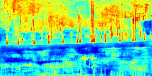
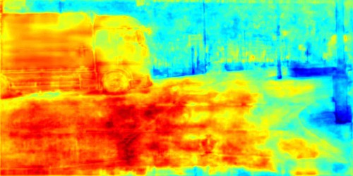
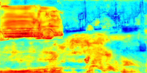
General classes. We visualize the learned Guided Attention for four representative classes in Figure 5. ‘Car’ and ‘Person’ are most common ‘thing’ classes in the Cityscapes dataset. ‘Building’ is a common ‘stuff’ class and ‘Pole’ is a common thin ‘stuff’ in Cityscapes. The activations are normalized between 0 (blue color) and 1 (red color).

From Figure 5, we observe several interesting behaviors:

• The guided attention learns localization of objects. The activations for ‘thing’ align quite well with the actual position of those objects.

• Guided attention focus on object co-occurrence. For example, ‘Car’ and ‘Person’ objects are usually on the road and the attentions for these classes learn to focus on both corresponding instances and road.

• Guided attention can find small objects. For example, there are multiple thin ‘Poles’ in the third row of Figure 5 and guided attention can find most of them.

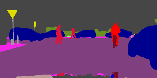
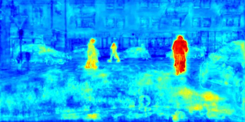
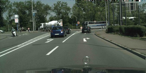
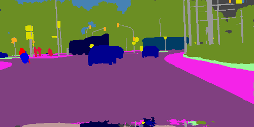
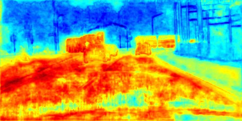
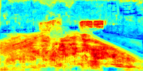
Semantically similar classes. We find guided attention is also capable of differentiating semantically similar classes. In Figure 6, we visualize the attention for two semantically similar classes: ‘Person’ and ‘Rider’. The attention for ‘Rider’ mainly fires for the rider instance on the right, and it does not fire for the two person instances on the left of the image. Our guided attention makes the features, passed to the next stage, more discriminative to semantically similar classes through the injected supervision, allowing our SPGNet to achieve better results on both ‘Person’ and ‘Rider’ classes than other state-of-the-art models, as shown in Table. 2.

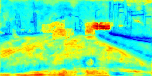
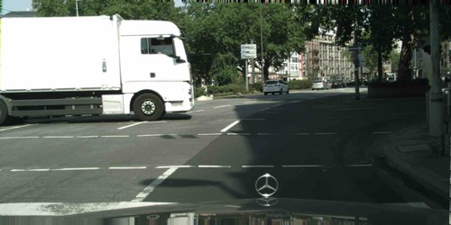
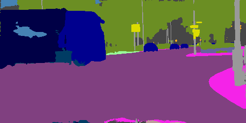
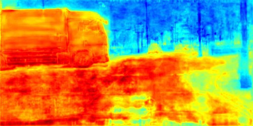
Failure cases. Our SPGNet confuses among ‘Truck’, ‘Bus’ and ‘Train’. We visualize the attentions for these classes in Figure 7. We observe that the Guided Attention maps for these classes usually activate together on the same object. It potentially produces features that are less discriminative to those classes, resulting in our worse performance on ‘Truck’, ‘Bus’ and ‘Train’, as shown in Table. 2.

4.6 Generalization to Other Datasets

Method	Extra data	Multi-scale	mIoU ($\%$)
Liang et al. [35]	✗	✓	63.57
Xia et al. [64]	✓	✓	64.39
Fang et al. [17]	✓	✓	67.60
DPC [6]	✗	✓	71.34
SPGNet (Ours)	✗	✗	67.23
SPGNet (Ours)	✗	✓	68.36

Table 10: Pascal Person-Part validation set performance.

To demonstrate that our model can be generalized to other datasets, we perform more experiments on the PASCAL VOC 2012 [16] and PASCAL Person-Part [12]. For both datasets, we follow the settings in [11] to train the model with a crop size of $513\times 513$, batch size of 28 for 30,000 iterations.

PASCAL VOC 2012: The SPGNet with a stack of 2 ResNet-50 achieves 77.33 mIoU. The performance of SPGNet is comparable with the current state-of-the-art ResNet-101 DeepLabV3+ [11] which achieves 77.37 mIoU with encoder stride=32 for a fair comparison.

PASCAL Person-Part: Table 10 shows comparison with state-of-the-art results on Pascal Person-Part. Our SPGNet with a stack of 2 ResNet-50 achieves 67.23 mIoU with a single scale input, and 68.36 mIoU with multi-scale inputs. Note that our SPGNet does not require extra MPII training data [2], as used in [64, 17].

5 Conclusion

We have proposed the SPGNet which demonstrates state-of-the-art performance for semantic segmentation on Cityscapes. Our proposed SPG module employs the ‘supervise-and-excite’ framework, where the local features are reweighted via the guidance from semantic prediction. The Guided Attention maps within the SPG module allows us to visually interpret the corresponding reweighting mechanism. Our experimental results show that a two-stage encoder-decoder network paired with our SPG module can significantly outperform its one-stage counterpart with similar parameters and computations. Finally, we plan to explore a more computationally efficient encoder-decoder structure for semantic segmentation in the future.

Acknowledgments

This work is in part supported by IBM-Illinois Center for Cognitive Computing Systems Research (C3SR) - a research collaboration as part of the IBM AI Horizons Network and Intelligence Advanced Research Projects Activity (IARPA) via contract D17PC00341, ARC DECRA DE190101315. The U.S. Government is authorized to reproduce and distribute reprints for Governmental purposes notwithstanding any copyright annotation thereon. Disclaimer: The views and conclusions contained herein are those of the authors and should not be interpreted as necessarily representing the official policies or endorsements, either expressed or implied, of IARPA, DOI/IBC, or the U.S. Government. The authors thank Samuel Rota Bulò and Peter Kontschieder for the valuable discussion about the global pooling kernel size.

Appendix A Extra Ablation Studies

We provide extra ablation studies on Cityscapes val set.

Effect of upsample module.

Upsample Module	mIoU ($\%$)	#Params	#FLOPs
FPN-style [37]	$70.01$	$11.5$M	$118.6$B
Ours	71.50	$11.6$M	$107.5$B

Table 11: Cityscapes val ablation studies on upsample module. All models use ResNet-18 in encoder. Our proposed upsample module requires fewer FLOPs and attains a better performance than the FPN-style upsample module.

We perform experiments to demonstrate the effectiveness of our proposed upsample module. We compare the decoder equipped with our proposed upsample module against the one using FPN-style upsample module [37] (i.e., bilinear upsample + residual blocks vs. nearest-neighbor upsample + single convolutions). In these experiments, we use ResNet-18 for encoder and we do not use global average pooling. For a fair comparison, we follow [37] to implement FPN decoder module and only use the largest resolution feature maps for prediction. We also add synchronized Inplace-ABN after all convolutions in our FPN implementation. Decoder channels are set to $128$ for both cases. Results are shown in Table 11. FPN-style upsample module and our proposed module have similar parameters but our upsample module requires $10$B fewer FLOPs than the FPN-style module, thanks to the bottleneck design in residual blocks. Furthermore, using our upsample module, the performance is almost $1.5$ mIoU better than the FPN-style upsample module.

Effect of global pooling.

GAP	Test Strategy	mIoU ($\%$)	#Params	#FLOPs
✗	-	$71.50$	$11.6$M	$107.5$B
✓	GAP	$72.87$	$11.7$M	$107.6$B
✓	TILED	$74.33$	$11.7$M	$8(\text{tiles})\times 30.6$B
✓	AP	74.48	$11.7$M	$107.6$B

Table 12: Cityscapes val ablation studies on global average pooling. All models use ResNet-18 in encoder. Adding global average pooling (GAP) is beneficial. Replacing GAP with average pooling (AP) is important during inference.

We experiment with the effect of Global Average Pooling (GAP) by using a single-stage encoder-decoder with ResNet-18 as encoder backbone. The GAP operation is deployed after the encoder features. The decoder module uses 128 channels.

We compare three strategies during inference:

1. GAP: Use global average pooling during inference on the $1024\times 2048$ image [39].

2. TILED: Crop overlapping patches within the image that have the same size as training crop size (e.g. $769\times 769$), and use $\frac{1}{3}$ overlap between patches (e.g., overlap with 256 pixels) [75].

3. AP: Replace global average pooling with an average pooling whose kernel size is the same as training crop size divided by the stride of that feature maps [47].

As shown in Table 12, we observe that using global average pooling (GAP) only improves the performance slightly by 1.3% due to the asymmetric setting during training and inference (i.e., train with crop size $769\times 769$ but inference with image size $1024\times 2048$). The TILED strategy resolves this problem by employing the same pooling kernel size during training and inference. However, it introduces extra computation since it requires processing redundant pixels within the overlapped regions among patches. Furthermore, it requires some heuristics to resolve the conflicts within the overlapped regions (e.g., average the predictions in the overlapped regions), which may lead to sub-optimal merging. On the other hand, the AP strategy is more efficient than the TILED strategy and performs slightly better, since no overlapped regions are processed.

References

- [1] Md Amirul Islam, Mrigank Rochan, Neil DB Bruce, and Yang Wang. Gated feedback refinement network for dense image labeling. In CVPR, 2017.
- [2] Mykhaylo Andriluka, Leonid Pishchulin, Peter Gehler, and Bernt Schiele. 2d human pose estimation: New benchmark and state of the art analysis. In CVPR, 2014.
- [3] Vijay Badrinarayanan, Alex Kendall, and Roberto Cipolla. Segnet: A deep convolutional encoder-decoder architecture for image segmentation. IEEE TPAMI, 2017.
- [4] Samuel Rota Bulò, Gerhard Neuhold, and Peter Kontschieder. Loss maxpooling for semantic image segmentation. In CVPR, 2017.
- [5] Zhe Cao, Tomas Simon, Shih-En Wei, and Yaser Sheikh. Realtime multi-person 2d pose estimation using part affinity fields. In CVPR, 2017.
- [6] Liang-Chieh Chen, Maxwell D. Collins, Yukun Zhu, George Papandreou, Barret Zoph, Florian Schroff, Hartwig Adam, and Jonathon Shlens. Searching for efficient multi-scale architectures for dense image prediction. In NIPS, 2018.
- [7] Liang-Chieh Chen, George Papandreou, Iasonas Kokkinos, Kevin Murphy, and Alan L Yuille. Semantic image segmentation with deep convolutional nets and fully connected crfs. In ICLR, 2015.
- [8] Liang-Chieh Chen, George Papandreou, Iasonas Kokkinos, Kevin Murphy, and Alan L Yuille. Deeplab: Semantic image segmentation with deep convolutional nets, atrous convolution, and fully connected crfs. IEEE TPAMI, 2017.
- [9] Liang-Chieh Chen, George Papandreou, Florian Schroff, and Hartwig Adam. Rethinking atrous convolution for semantic image segmentation. arXiv preprint arXiv:1706.05587, 2017.
- [10] Liang-Chieh Chen, Yi Yang, Jiang Wang, Wei Xu, and Alan L Yuille. Attention to scale: Scale-aware semantic image segmentation. In CVPR, 2016.
- [11] Liang-Chieh Chen, Yukun Zhu, George Papandreou, Florian Schroff, and Hartwig Adam. Encoder-decoder with atrous separable convolution for semantic image segmentation. In ECCV, 2018.
- [12] Xianjie Chen, Roozbeh Mottaghi, Xiaobai Liu, Sanja Fidler, Raquel Urtasun, and Alan Yuille. Detect what you can: Detecting and representing objects using holistic models and body parts. In CVPR, pages 1971–1978, 2014.
- [13] Yunpeng Chen, Yannis Kalantidis, Jianshu Li, Shuicheng Yan, and Jiashi Feng. A^ 2-nets: Double attention networks. In NIPS, 2018.
- [14] Marius Cordts, Mohamed Omran, Sebastian Ramos, Timo Rehfeld, Markus Enzweiler, Rodrigo Benenson, Uwe Franke, Stefan Roth, and Bernt Schiele. The cityscapes dataset for semantic urban scene understanding. In CVPR, 2016.
- [15] Jia Deng, Wei Dong, Richard Socher, Li-Jia Li, Kai Li, and Li Fei-Fei. Imagenet: A large-scale hierarchical image database. In CVPR, 2009.
- [16] M. Everingham, L. Van Gool, C. K. I. Williams, J. Winn, and A. Zisserman. The pascal visual object classes (voc) challenge. IJCV, 2010.
- [17] Hao-Shu Fang, Guansong Lu, Xiaolin Fang, Jianwen Xie, Yu-Wing Tai, and Cewu Lu. Weakly and semi supervised human body part parsing via pose-guided knowledge transfer. arXiv preprint arXiv:1805.04310, 2018.
- [18] Jun Fu, Jing Liu, Haijie Tian, Yong Li, Yongjun Bao, Zhiwei Fang, and Hanqing Lu. Dual attention network for scene segmentation. In CVPR, 2019.
- [19] Jun Fu, Jing Liu, Yuhang Wang, Jin Zhou, Changyong Wang, and Hanqing Lu. Stacked deconvolutional network for semantic segmentation. IEEE TIP, 2019.
- [20] Kaiming He, Xiangyu Zhang, Shaoqing Ren, and Jian Sun. Deep residual learning for image recognition. In CVPR, 2016.
- [21] Xuming He, Richard S. Zemel, and Miguel Á. Carreira-Perpiñán. Multiscale conditional random fields for image labeling. In CVPR, 2004.
- [22] Matthias Holschneider, Richard Kronland-Martinet, Jean Morlet, and Ph Tchamitchian. A real-time algorithm for signal analysis with the help of the wavelet transform. In Wavelets: Time-Frequency Methods and Phase Space, pages 289–297. 1989.
- [23] Han Hu, Jiayuan Gu, Zheng Zhang, Jifeng Dai, and Yichen Wei. Relation networks for object detection. In CVPR, 2018.
- [24] Jie Hu, Li Shen, Samuel Albanie, Gang Sun, and Andrea Vedaldi. Gather-excite: Exploiting feature context in convolutional neural networks. In NIPS, 2018.
- [25] Jie Hu, Li Shen, and Gang Sun. Squeeze-and-excitation networks. In CVPR, 2018.
- [26] Zilong Huang, Xinggang Wang, Lichao Huang, Chang Huang, Yunchao Wei, and Wenyu Liu. Ccnet: Criss-cross attention for semantic segmentation. In ICCV, 2019.
- [27] Jianbo Jiao, Yunchao Wei, Zequn Jie, Honghui Shi, Rynson WH Lau, and Thomas S Huang. Geometry-aware distillation for indoor semantic segmentation. In CVPR, 2019.
- [28] Lipeng Ke, Ming-Ching Chang, Honggang Qi, and Siwei Lyu. Multi-scale structure-aware network for human pose estimation. In ECCV, 2018.
- [29] Shu Kong and Charless C Fowlkes. Recurrent scene parsing with perspective understanding in the loop. In CVPR, 2018.
- [30] Alex Krizhevsky, Ilya Sutskever, and Geoffrey E Hinton. Imagenet classification with deep convolutional neural networks. In NIPS, 2012.
- [31] L’ubor Ladickỳ, Paul Sturgess, Karteek Alahari, Chris Russell, and Philip HS Torr. What, where and how many? combining object detectors and crfs. In ECCV, 2010.
- [32] Yann LeCun, Bernhard Boser, John S Denker, Donnie Henderson, Richard E Howard, Wayne Hubbard, and Lawrence D Jackel. Backpropagation applied to handwritten zip code recognition. Neural computation, 1(4):541–551, 1989.
- [33] Wenbo Li, Zhicheng Wang, Binyi Yin, Qixiang Peng, Yuming Du, Tianzi Xiao, Gang Yu, Hongtao Lu, Yichen Wei, and Jian Sun. Rethinking on multi-stage networks for human pose estimation. arXiv preprint arXiv:1901.00148, 2019.
- [34] Xiaoxiao Li, Ziwei Liu, Ping Luo, Chen Change Loy, and Xiaoou Tang. Not all pixels are equal: Difficulty-aware semantic segmentation via deep layer cascade. In CVPR, 2017.
- [35] Xiaodan Liang, Liang Lin, Xiaohui Shen, Jiashi Feng, Shuicheng Yan, and Eric P Xing. Interpretable structure-evolving lstm. In CVPR, 2017.
- [36] Guosheng Lin, Anton Milan, Chunhua Shen, and Ian Reid. Refinenet: Multi-path refinement networks for high-resolution semantic segmentation. In CVPR, 2017.
- [37] Tsung-Yi Lin, Piotr Dollár, Ross Girshick, Kaiming He, Bharath Hariharan, and Serge Belongie. Feature pyramid networks for object detection. In CVPR, 2017.
- [38] Chenxi Liu, Liang-Chieh Chen, Florian Schroff, Hartwig Adam, Wei Hua, Alan Yuille, and Li Fei-Fei. Auto-deeplab: Hierarchical neural architecture search for semantic image segmentation. arXiv preprint arXiv:1901.02985, 2019.
- [39] Wei Liu, Andrew Rabinovich, and Alexander C Berg. Parsenet: Looking wider to see better. arXiv:1506.04579, 2015.
- [40] Jonathan Long, Evan Shelhamer, and Trevor Darrell. Fully convolutional networks for semantic segmentation. In IEEE TPAMI, 2015.
- [41] Alejandro Newell, Zhiao Huang, and Jia Deng. Associative embedding: End-to-end learning for joint detection and grouping. In NIPS, 2017.
- [42] Alejandro Newell, Kaiyu Yang, and Jia Deng. Stacked hourglass networks for human pose estimation. In ECCV, 2016.
- [43] Hyeonwoo Noh, Seunghoon Hong, and Bohyung Han. Learning deconvolution network for semantic segmentation. In ICCV, 2015.
- [44] George Papandreou, Iasonas Kokkinos, and Pierre-Andre Savalle. Modeling local and global deformations in deep learning: Epitomic convolution, multiple instance learning, and sliding window detection. In CVPR, 2015.
- [45] Chao Peng, Xiangyu Zhang, Gang Yu, Guiming Luo, and Jian Sun. Large kernel matters–improve semantic segmentation by global convolutional network. In CVPR, 2017.
- [46] Tobias Pohlen, Alexander Hermans, Markus Mathias, and Bastian Leibe. Full-resolution residual networks for semantic segmentation in street scenes. In CVPR, 2017.
- [47] Lorenzo Porzi, Samuel Rota Bulo, Aleksander Colovic, and Peter Kontschieder. Seamless scene segmentation. In CVPR, 2019.
- [48] Olaf Ronneberger, Philipp Fischer, and Thomas Brox. U-net: Convolutional networks for biomedical image segmentation. In MICCAI. Springer, 2015.
- [49] Samuel Rota Bulò, Lorenzo Porzi, and Peter Kontschieder. In-place activated batchnorm for memory-optimized training of dnns. In CVPR, 2018.
- [50] Pierre Sermanet, David Eigen, Xiang Zhang, Michaël Mathieu, Rob Fergus, and Yann LeCun. Overfeat: Integrated recognition, localization and detection using convolutional networks. arXiv preprint arXiv:1312.6229, 2013.
- [51] Sohil Shah, Pallabi Ghosh, Larry S Davis, and Tom Goldstein. Stacked u-nets: a no-frills approach to natural image segmentation. arXiv preprint arXiv:1804.10343, 2018.
- [52] Karen Simonyan and Andrew Zisserman. Very deep convolutional networks for large-scale image recognition. In ICLR, 2015.
- [53] Yuhang Song, Chao Yang, Yeji Shen, Peng Wang, Qin Huang, and C-C Jay Kuo. Spg-net: Segmentation prediction and guidance network for image inpainting. arXiv preprint arXiv:1805.03356, 2018.
- [54] Christian Szegedy, Wei Liu, Yangqing Jia, Pierre Sermanet, Scott Reed, Dragomir Anguelov, Dumitru Erhan, Vincent Vanhoucke, and Andrew Rabinovich. Going deeper with convolutions. In CVPR, 2015.
- [55] Joseph Tighe and Svetlana Lazebnik. Finding things: Image parsing with regions and per-exemplar detectors. In CVPR, 2013.
- [56] Zhuowen Tu, Xiangrong Chen, Alan L Yuille, and Song-Chun Zhu. Image parsing: Unifying segmentation, detection, and recognition. IJCV, 2005.
- [57] Ashish Vaswani, Noam Shazeer, Niki Parmar, Jakob Uszkoreit, Llion Jones, Aidan N Gomez, Łukasz Kaiser, and Illia Polosukhin. Attention is all you need. In NIPS, 2017.
- [58] Panqu Wang, Pengfei Chen, Ye Yuan, Ding Liu, Zehua Huang, Xiaodi Hou, and Garrison Cottrell. Understanding convolution for semantic segmentation. In WACV, 2018.
- [59] Tiantian Wang, Ali Borji, Lihe Zhang, Pingping Zhang, and Huchuan Lu. A stagewise refinement model for detecting salient objects in images. In ICCV, 2017.
- [60] Xiaolong Wang, Ross Girshick, Abhinav Gupta, and Kaiming He. Non-local neural networks. In CVPR, 2018.
- [61] Shih-En Wei, Varun Ramakrishna, Takeo Kanade, and Yaser Sheikh. Convolutional pose machines. In CVPR, 2016.
- [62] Zbigniew Wojna, Vittorio Ferrari, Sergio Guadarrama, Nathan Silberman, Liang-Chieh Chen, Alireza Fathi, and Jasper Uijlings. The devil is in the decoder: Classification, regression and gans. IJCV, pages 1–13, 2019.
- [63] Zifeng Wu, Chunhua Shen, and Anton van den Hengel. Bridging category-level and instance-level semantic image segmentation. arXiv:1605.06885, 2016.
- [64] Fangting Xia, Peng Wang, Xianjie Chen, and Alan L Yuille. Joint multi-person pose estimation and semantic part segmentation. In CVPR, 2017.
- [65] Tete Xiao, Yingcheng Liu, Bolei Zhou, Yuning Jiang, and Jian Sun. Unified perceptual parsing for scene understanding. In ECCV, 2018.
- [66] Maoke Yang, Kun Yu, Chi Zhang, Zhiwei Li, and Kuiyuan Yang. Denseaspp for semantic segmentation in street scenes. In CVPR, 2018.
- [67] Tien-Ju Yang, Maxwell D Collins, Yukun Zhu, Jyh-Jing Hwang, Ting Liu, Xiao Zhang, Vivienne Sze, George Papandreou, and Liang-Chieh Chen. Deeperlab: Single-shot image parser. arXiv preprint arXiv:1902.05093, 2019.
- [68] Wei Yang, Shuang Li, Wanli Ouyang, Hongsheng Li, and Xiaogang Wang. Learning feature pyramids for human pose estimation. In ICCV, 2017.
- [69] Jian Yao, Sanja Fidler, and Raquel Urtasun. Describing the scene as a whole: Joint object detection, scene classification and semantic segmentation. In CVPR, 2012.
- [70] Changqian Yu, Jingbo Wang, Chao Peng, Changxin Gao, Gang Yu, and Nong Sang. Bisenet: Bilateral segmentation network for real-time semantic segmentation. In ECCV, 2018.
- [71] Changqian Yu, Jingbo Wang, Chao Peng, Changxin Gao, Gang Yu, and Nong Sang. Learning a discriminative feature network for semantic segmentation. In CVPR, 2018.
- [72] Hang Zhang, Kristin Dana, Jianping Shi, Zhongyue Zhang, Xiaogang Wang, Ambrish Tyagi, and Amit Agrawal. Context encoding for semantic segmentation. In CVPR, 2018.
- [73] Rui Zhang, Sheng Tang, Yongdong Zhang, Jintao Li, and Shuicheng Yan. Scale-adaptive convolutions for scene parsing. In ICCV, 2017.
- [74] Zhenli Zhang, Xiangyu Zhang, Chao Peng, Xiangyang Xue, and Jian Sun. Exfuse: Enhancing feature fusion for semantic segmentation. In ECCV, 2018.
- [75] Hengshuang Zhao, Jianping Shi, Xiaojuan Qi, Xiaogang Wang, and Jiaya Jia. Pyramid scene parsing network. In CVPR, 2017.
- [76] Hengshuang Zhao, Yi Zhang, Shu Liu, Jianping Shi, Chen Change Loy, Dahua Lin, and Jiaya Jia. Psanet: Point-wise spatial attention network for scene parsing. In ECCV, 2018.
- [77] Bolei Zhou, Hang Zhao, Xavier Puig, Sanja Fidler, Adela Barriuso, and Antonio Torralba. Scene parsing through ade20k dataset. In CVPR, 2017.
- [78] Barret Zoph and Quoc V. Le. Neural architecture search with reinforcement learning. In ICLR, 2017.