Once-for-All: Train One Network and Specialize it for Efficient Deployment
Abstract
We address the challenging problem of efficient inference across many devices and resource constraints, especially on edge devices. Conventional approaches either manually design or use neural architecture search (NAS) to find a specialized neural network and train it from scratch for each case, which is computationally prohibitive (causing emission as much as 5 cars’ lifetime Strubell et al. (2019)) thus unscalable. In this work, we propose to train a once-for-all (OFA) network that supports diverse architectural settings by decoupling training and search, to reduce the cost. We can quickly get a specialized sub-network by selecting from the OFA network without additional training. To efficiently train OFA networks, we also propose a novel progressive shrinking algorithm, a generalized pruning method that reduces the model size across many more dimensions than pruning (depth, width, kernel size, and resolution). It can obtain a surprisingly large number of sub-networks () that can fit different hardware platforms and latency constraints while maintaining the same level of accuracy as training independently. On diverse edge devices, OFA consistently outperforms state-of-the-art (SOTA) NAS methods (up to 4.0% ImageNet top1 accuracy improvement over MobileNetV3, or same accuracy but 1.5 faster than MobileNetV3, 2.6 faster than EfficientNet w.r.t measured latency) while reducing many orders of magnitude GPU hours and emission. In particular, OFA achieves a new SOTA 80.0% ImageNet top-1 accuracy under the mobile setting (600M MACs). OFA is the winning solution for the 3rd Low Power Computer Vision Challenge (LPCVC), DSP classification track and the 4th LPCVC, both classification track and detection track. Code and 50 pre-trained models (for many devices & many latency constraints) are released at https://github.com/mit-han-lab/once-for-all.
1 Introduction
Deep Neural Networks (DNNs) deliver state-of-the-art accuracy in many machine learning applications. However, the explosive growth in model size and computation cost gives rise to new challenges on how to efficiently deploy these deep learning models on diverse hardware platforms, since they have to meet different hardware efficiency constraints (e.g., latency, energy). For instance, one mobile application on App Store has to support a diverse range of hardware devices, from a high-end Samsung Note10 with a dedicated neural network accelerator to a 5-year-old Samsung S6 with a much slower processor. With different hardware resources (e.g., on-chip memory size, #arithmetic units), the optimal neural network architecture varies significantly. Even running on the same hardware, under different battery conditions or workloads, the best model architecture also differs a lot.

Given different hardware platforms and efficiency constraints (defined as deployment scenarios), researchers either design compact models specialized for mobile (Howard et al., 2017; Sandler et al., 2018; Zhang et al., 2018) or accelerate the existing models by compression (Han et al., 2016; He et al., 2018) for efficient deployment. However, designing specialized DNNs for every scenario is engineer-expensive and computationally expensive, either with human-based methods or NAS. Since such methods need to repeat the network design process and retrain the designed network from scratch for each case. Their total cost grows linearly as the number of deployment scenarios increases, which will result in excessive energy consumption and emission (Strubell et al., 2019). It makes them unable to handle the vast amount of hardware devices (23.14 billion IoT devices till 2018111https://www.statista.com/statistics/471264/iot-number-of-connected-devices-worldwide/) and highly dynamic deployment environments (different battery conditions, different latency requirements, etc.).
This paper introduces a new solution to tackle this challenge – designing a once-for-all network that can be directly deployed under diverse architectural configurations, amortizing the training cost. The inference is performed by selecting only part of the once-for-all network. It flexibly supports different depths, widths, kernel sizes, and resolutions without retraining. A simple example of Once-for-All (OFA) is illustrated in Figure 1 (left). Specifically, we decouple the model training stage and the neural architecture search stage. In the model training stage, we focus on improving the accuracy of all sub-networks that are derived by selecting different parts of the once-for-all network. In the model specialization stage, we sample a subset of sub-networks to train an accuracy predictor and latency predictors. Given the target hardware and constraint, a predictor-guided architecture search (Liu et al., 2018) is conducted to get a specialized sub-network, and the cost is negligible. As such, we reduce the total cost of specialized neural network design from O(N) to O(1) (Figure 1 middle).
However, training the once-for-all network is a non-trivial task, since it requires joint optimization of the weights to maintain the accuracy of a large number of sub-networks (more than 1019 in our experiments). It is computationally prohibitive to enumerate all sub-networks to get the exact gradient in each update step, while randomly sampling a few sub-networks in each step will lead to significant accuracy drops. The challenge is that different sub-networks are interfering with each other, making the training process of the whole once-for-all network inefficient. To address this challenge, we propose a progressive shrinking algorithm for training the once-for-all network. Instead of directly optimizing the once-for-all network from scratch, we propose to first train the largest neural network with maximum depth, width, and kernel size, then progressively fine-tune the once-for-all network to support smaller sub-networks that share weights with the larger ones. As such, it provides better initialization by selecting the most important weights of larger sub-networks, and the opportunity to distill smaller sub-networks, which greatly improves the training efficiency. From this perspective, progressive shrinking can be viewed as a generalized network pruning method that shrinks multiple dimensions (depth, width, kernel size, and resolution) of the full network rather than only the width dimension. Besides, it targets on maintaining the accuracy of all sub-networks rather than a single pruned network.
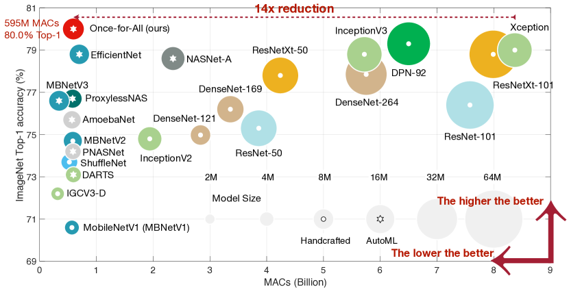
We extensively evaluated the effectiveness of OFA on ImageNet with many hardware platforms (CPU, GPU, mCPU, mGPU, FPGA accelerator) and efficiency constraints. Under all deployment scenarios, OFA consistently improves the ImageNet accuracy by a significant margin compared to SOTA hardware-aware NAS methods while saving the GPU hours, dollars, and emission by orders of magnitude. On the ImageNet mobile setting (less than 600M MACs), OFA achieves a new SOTA 80.0% top1 accuracy with 595M MACs (Figure 2). To the best of our knowledge, this is the first time that the SOTA ImageNet top1 accuracy reaches 80% under the mobile setting.
2 Related Work
Efficient Deep Learning.
Many efficient neural network architectures are proposed to improve the hardware efficiency, such as SqueezeNet (Iandola et al., 2016), MobileNets (Howard et al., 2017; Sandler et al., 2018), ShuffleNets (Ma et al., 2018; Zhang et al., 2018), etc. Orthogonal to architecting efficient neural networks, model compression (Han et al., 2016) is another very effective technique for efficient deep learning, including network pruning that removes redundant units (Han et al., 2015) or redundant channels (He et al., 2018; Liu et al., 2017), and quantization that reduces the bit width for the weights and activations (Han et al., 2016; Courbariaux et al., 2015; Zhu et al., 2017).
Neural Architecture Search.
Neural architecture search (NAS) focuses on automating the architecture design process (Zoph & Le, 2017; Zoph et al., 2018; Real et al., 2019; Cai et al., 2018a; Liu et al., 2019). Early NAS methods (Zoph et al., 2018; Real et al., 2019; Cai et al., 2018b) search for high-accuracy architectures without taking hardware efficiency into consideration. Therefore, the produced architectures (e.g., NASNet, AmoebaNet) are not efficient for inference. Recent hardware-aware NAS methods (Cai et al., 2019; Tan et al., 2019; Wu et al., 2019) directly incorporate the hardware feedback into architecture search. Hardware-DNN co-design techniques (Jiang et al., 2019b; a; Hao et al., 2019) jointly optimize neural network architectures and hardware architectures. As a result, they can improve inference efficiency. However, given new inference hardware platforms, these methods need to repeat the architecture search process and retrain the model, leading to prohibitive GPU hours, dollars, and emission. They are not scalable to a large number of deployment scenarios. The individually trained models do not share any weight, leading to large total model size and high downloading bandwidth.
Dynamic Neural Networks.
To improve the efficiency of a given neural network, some work explored skipping part of the model based on the input image. For example, Wu et al. (2018); Liu & Deng (2018); Wang et al. (2018) learn a controller or gating modules to adaptively drop layers; Huang et al. (2018) introduce early-exit branches in the computation graph; Lin et al. (2017) adaptively prune channels based on the input feature map; Kuen et al. (2018) introduce stochastic downsampling point to reduce the feature map size adaptively. Recently, Slimmable Nets (Yu et al., 2019; Yu & Huang, 2019b) propose to train a model to support multiple width multipliers (e.g., 4 different global width multipliers), building upon existing human-designed neural networks (e.g., MobileNetV2 0.35, 0.5, 0.75, 1.0). Such methods can adaptively fit different efficiency constraints at runtime, however, still inherit a pre-designed neural network (e.g., MobileNet-v2), which limits the degree of flexibility (e.g., only width multiplier can adapt) and the ability in handling new deployment scenarios where the pre-designed neural network is not optimal. In this work, in contrast, we enable a much more diverse architecture space (depth, width, kernel size, and resolution) and a significantly larger number of architectural settings ( v.s. 4 (Yu et al., 2019)). Thanks to the diversity and the large design space, we can derive new specialized neural networks for many different deployment scenarios rather than working on top of an existing neural network that limits the optimization headroom. However, it is more challenging to train the network to achieve this flexibility, which motivates us to design the progressive shrinking algorithm to tackle this challenge.
3 Method
3.1 Problem Formalization
Assuming the weights of the once-for-all network as and the architectural configurations as , we then can formalize the problem as
| (1) |
where denotes a selection scheme that selects part of the model from the once-for-all network to form a sub-network with architectural configuration . The overall training objective is to optimize to make each supported sub-network maintain the same level of accuracy as independently training a network with the same architectural configuration.
3.2 Architecture Space
Our once-for-all network provides one model but supports many sub-networks of different sizes, covering four important dimensions of the convolutional neural networks (CNNs) architectures, i.e., depth, width, kernel size, and resolution. Following the common practice of many CNN models (He et al., 2016; Sandler et al., 2018; Huang et al., 2017), we divide a CNN model into a sequence of units with gradually reduced feature map size and increased channel numbers. Each unit consists of a sequence of layers where only the first layer has stride 2 if the feature map size decreases (Sandler et al., 2018). All the other layers in the units have stride 1.
We allow each unit to use arbitrary numbers of layers (denoted as elastic depth); For each layer, we allow to use arbitrary numbers of channels (denoted as elastic width) and arbitrary kernel sizes (denoted as elastic kernel size). In addition, we also allow the CNN model to take arbitrary input image sizes (denoted as elastic resolution). For example, in our experiments, the input image size ranges from 128 to 224 with a stride 4; the depth of each unit is chosen from {2, 3, 4}; the width expansion ratio in each layer is chosen from {3, 4, 6}; the kernel size is chosen from {3, 5, 7}. Therefore, with 5 units, we have roughly different neural network architectures and each of them can be used under 25 different input resolutions. Since all of these sub-networks share the same weights (i.e., ) (Cheung et al., 2019), we only require 7.7M parameters to store all of them. Without sharing, the total model size will be prohibitive.
3.3 Training the Once-for-all Network

Naïve Approach.
Training the once-for-all network can be cast as a multi-objective problem, where each objective corresponds to one sub-network. From this perspective, a naïve training approach is to directly optimize the once-for-all network from scratch using the exact gradient of the overall objective, which is derived by enumerating all sub-networks in each update step, as shown in Eq. (1). The cost of this approach is linear to the number of sub-networks. Therefore, it is only applicable to scenarios where a limited number of sub-networks are supported (Yu et al., 2019), while in our case, it is computationally prohibitive to adopt this approach.
Another naïve training approach is to sample a few sub-networks in each update step rather than enumerate all of them, which does not have the issue of prohibitive cost. However, with such a large number of sub-networks that share weights, thus interfere with each other, we find it suffers from significant accuracy drop. In the following section, we introduce a solution to address this challenge, i.e., progressive shrinking.
Progressive Shrinking.
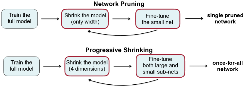
The once-for-all network comprises many sub-networks of different sizes where small sub-networks are nested in large sub-networks. To prevent interference between the sub-networks, we propose to enforce a training order from large sub-networks to small sub-networks in a progressive manner. We name this training scheme as progressive shrinking (PS). An example of the training process with PS is provided in Figure 3 and Figure 4, where we start with training the largest neural network with the maximum kernel size (e.g., 7), depth (e.g., 4), and width (e.g., 6). Next, we progressively fine-tune the network to support smaller sub-networks by gradually adding them into the sampling space (larger sub-networks may also be sampled). Specifically, after training the largest network, we first support elastic kernel size which can choose from {3, 5, 7} at each layer, while the depth and width remain the maximum values. Then, we support elastic depth and elastic width sequentially, as is shown in Figure 3. The resolution is elastic throughout the whole training process, which is implemented by sampling different image sizes for each batch of training data. We also use the knowledge distillation technique after training the largest neural network (Hinton et al., 2015; Ashok et al., 2018; Yu & Huang, 2019b). It combines two loss terms using both the soft labels given by the largest neural network and the real labels.
Compared to the naïve approach, PS prevents small sub-networks from interfering large sub-networks, since large sub-networks are already well-trained when the once-for-all network is fine-tuned to support small sub-networks. Regarding the small sub-networks, they share the weights with the large ones. Therefore, PS allows initializing small sub-networks with the most important weights of well-trained large sub-networks, which expedites the training process. Compared to network pruning (Figure 4), PS also starts with training the full model, but it shrinks not only the width dimension but also the depth, kernel size, and resolution dimensions of the full model. Additionally, PS fine-tunes both large and small sub-networks rather than a single pruned network. As a result, PS provides a much more powerful once-for-all network that can fit diverse hardware platforms and efficiency constraints compared to network pruning. We describe the details of the PS training flow as follows:


-
•
Elastic Kernel Size (Figure 5 left). We let the center of a 7x7 convolution kernel also serve as a 5x5 kernel, the center of which can also be a 3x3 kernel. Therefore, the kernel size becomes elastic. The challenge is that the centering sub-kernels (e.g., 3x3 and 5x5) are shared and need to play multiple roles (independent kernel and part of a large kernel). The weights of centered sub-kernels may need to have different distribution or magnitude as different roles. Forcing them to be the same degrades the performance of some sub-networks. Therefore, we introduce kernel transformation matrices when sharing the kernel weights. We use separate kernel transformation matrices for different layers. Within each layer, the kernel transformation matrices are shared among different channels. As such, we only need extra parameters to store the kernel transformation matrices in each layer, which is negligible.
-
•
Elastic Depth (Figure 5 right). To derive a sub-network that has layers in a unit that originally has layers, we keep the first D layers and skip the last layers, rather than keeping any layers as done in current NAS methods (Cai et al., 2019; Wu et al., 2019). As such, one depth setting only corresponds to one combination of layers. In the end, the weights of the first D layers are shared between large and small models.
-
•
Elastic Width (Figure 6). Width means the number of channels. We give each layer the flexibility to choose different channel expansion ratios. Following the progressive shrinking scheme, we first train a full-width model. Then we introduce a channel sorting operation to support partial widths. It reorganizes the channels according to their importance, which is calculated based on the L1 norm of a channel’s weight. Larger L1 norm means more important. For example, when shrinking from a 4-channel-layer to a 3-channel-layer, we select the largest 3 channels, whose weights are shared with the 4-channel-layer (Figure 6 left and middle). Thereby, smaller sub-networks are initialized with the most important channels on the once-for-all network which is already well trained. This channel sorting operation preserves the accuracy of larger sub-networks.
3.4 Specialized Model Deployment with Once-for-all Network
Having trained a once-for-all network, the next stage is to derive the specialized sub-network for a given deployment scenario. The goal is to search for a neural network that satisfies the efficiency (e.g., latency, energy) constraints on the target hardware while optimizing the accuracy. Since OFA decouples model training from neural architecture search, we do not need any training cost in this stage. Furthermore, we build neural-network-twins to predict the latency and accuracy given a neural network architecture, providing a quick feedback for model quality. It eliminates the repeated search cost by substituting the measured accuracy/latency with predicted accuracy/latency (twins).
Specifically, we randomly sample 16K sub-networks with different architectures and input image sizes, then measure their accuracy on 10K validation images sampled from the original training set. These [architecture, accuracy] pairs are used to train an accuracy predictor to predict the accuracy of a model given its architecture and input image size222Details of the accuracy predictor is provided in Appendix A.. We also build a latency lookup table (Cai et al., 2019) on each target hardware platform to predict the latency. Given the target hardware and latency constraint, we conduct an evolutionary search (Real et al., 2019) based on the neural-network-twins to get a specialized sub-network. Since the cost of searching with neural-network-twins is negligible, we only need 40 GPU hours to collect the data pairs, and the cost stays constant regardless of #deployment scenarios.
4 Experiments
In this section, we first apply the progressive shrinking algorithm to train the once-for-all network on ImageNet (Deng et al., 2009). Then we demonstrate the effectiveness of our trained once-for-all network on various hardware platforms (Samsung S7 Edge, Note8, Note10, Google Pixel1, Pixel2, LG G8, NVIDIA 1080Ti, V100 GPUs, Jetson TX2, Intel Xeon CPU, Xilinx ZU9EG, and ZU3EG FPGAs) with different latency constraints.
4.1 Training the Once-for-all Network on ImageNet
Training Details.
We use the same architecture space as MobileNetV3 (Howard et al., 2019). For training the full network, we use the standard SGD optimizer with Nesterov momentum 0.9 and weight decay . The initial learning rate is 2.6, and we use the cosine schedule (Loshchilov & Hutter, 2016) for learning rate decay. The full network is trained for 180 epochs with batch size 2048 on 32 GPUs. Then we follow the schedule described in Figure 3 to further fine-tune the full network333Implementation details can be found in Appendix B.. The whole training process takes around 1,200 GPU hours on V100 GPUs. This is a one-time training cost that can be amortized by many deployment scenarios.
Results.
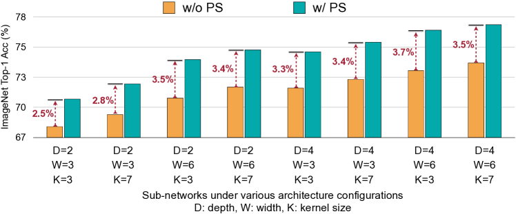
Figure 7 reports the top1 accuracy of sub-networks derived from the once-for-all networks that are trained with our progressive shrinking (PS) algorithm and without PS respectively. Due to space limits, we take 8 sub-networks for comparison, and each of them is denoted as “(D = , W = , K = )”. It represents a sub-network that has layers for all units, while the expansion ratio and kernel size are set to and for all layers. PS can improve the ImageNet accuracy of sub-networks by a significant margin under all architectural settings. Specifically, without architecture optimization, PS can achieve 74.8% top1 accuracy using 226M MACs under the architecture setting (D=4, W=3, K=3), which is on par with MobileNetV3-Large. In contrast, without PS, it only achieves 71.5%, which is 3.3% lower.
4.2 Specialized Sub-networks for Different Hardware and Constraints
We apply our trained once-for-all network to get different specialized sub-networks for diverse hardware platforms: from the cloud to the edge. On cloud devices, the latency for GPU is measured with batch size 64 on NVIDIA 1080Ti and V100 with Pytorch 1.0+cuDNN. The CPU latency is measured with batch size 1 on Intel Xeon E5-2690 v4+MKL-DNN. On edge devices, including mobile phones, we use Samsung, Google and LG phones with TF-Lite, batch size 1; for mobile GPU, we use Jetson TX2 with Pytorch 1.0+cuDNN, batch size of 16; for embedded FPGA, we use Xilinx ZU9EG and ZU3EG FPGAs with Vitis AI444https://www.xilinx.com/products/design-tools/vitis/vitis-ai.html, batch size 1.
| Model | ImageNet | MACs | Mobile | Search cost | Training cost | Total cost | ||
| Top1 (%) | latency | (GPU hours) | (GPU hours) | GPU hours | e (lbs) | AWS cost | ||
| MobileNetV2 [31] | 72.0 | 300M | 66ms | 0 | 150 | 6k | 1.7k | $18.4k |
| MobileNetV2 #1200 | 73.5 | 300M | 66ms | 0 | 1200 | 48k | 13.6k | $146.9k |
| NASNet-A [44] | 74.0 | 564M | - | 48,000 | - | 1,920k | 544.5k | $5875.2k |
| DARTS [25] | 73.1 | 595M | - | 96 | 250 | 14k | 4.0k | $42.8k |
| MnasNet [33] | 74.0 | 317M | 70ms | 40,000 | - | 1,600k | 453.8k | $4896.0k |
| FBNet-C [36] | 74.9 | 375M | - | 216 | 360 | 23k | 6.5k | $70.4k |
| ProxylessNAS [4] | 74.6 | 320M | 71ms | 200 | 300 | 20k | 5.7k | $61.2k |
| SinglePathNAS [8] | 74.7 | 328M | - | 288 + 24 | 384 | 17k | 4.8k | $52.0k |
| AutoSlim [38] | 74.2 | 305M | 63ms | 180 | 300 | 12k | 3.4k | $36.7k |
| MobileNetV3-Large [15] | 75.2 | 219M | 58ms | - | 180 | 7.2k | 1.8k | $22.2k |
| OFA w/o PS | 72.4 | 235M | 59ms | 40 | 1200 | 1.2k | 0.34k | $3.7k |
| OFA w/ PS | 76.0 | 230M | 58ms | 40 | 1200 | 1.2k | 0.34k | $3.7k |
| OFA w/ PS #25 | 76.4 | 230M | 58ms | 40 | 1200 + 25 | 2.2k | 0.62k | $6.7k |
| OFA w/ PS #75 | 76.9 | 230M | 58ms | 40 | 1200 + 75 | 4.2k | 1.2k | $13.0k |
| OFA w/ PS #75 | 80.0 | 595M | - | 40 | 1200 + 75 | 4.2k | 1.2k | $13.0k |

Comparison with NAS on Mobile Devices.
Table 1 reports the comparison between OFA and state-of-the-art hardware-aware NAS methods on the mobile phone (Pixel1). OFA is much more efficient than NAS when handling multiple deployment scenarios since the cost of OFA is constant while others are linear to the number of deployment scenarios (). With = 40, the total emissions of OFA is 16 fewer than ProxylessNAS, 19 fewer than FBNet, and 1,300 fewer than MnasNet (Figure 8). Without retraining, OFA achieves 76.0% top1 accuracy on ImageNet, which is 0.8% higher than MobileNetV3-Large while maintaining similar mobile latency. We can further improve the top1 accuracy to 76.4% by fine-tuning the specialized sub-network for 25 epochs and to 76.9% by fine-tuning for 75 epochs. Besides, we also observe that OFA with PS can achieve 3.6% better accuracy than without PS.
OFA under Different Computational Resource Constraints.
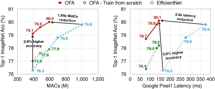
Figure 9 summarizes the results of OFA under different MACs and Pixel1 latency constraints. OFA achieves 79.1% ImageNet top1 accuracy with 389M MACs, being 2.8% more accurate than EfficientNet-B0 that has similar MACs. With 595M MACs, OFA reaches a new SOTA 80.0% ImageNet top1 accuracy under the mobile setting (600M MACs), which is 0.2% higher than EfficientNet-B2 while using 1.68 fewer MACs. More importantly, OFA runs much faster than EfficientNets on hardware. Specifically, with 143ms Pixel1 latency, OFA achieves 80.1% ImageNet top1 accuracy, being 0.3% more accurate and 2.6 faster than EfficientNet-B2. We also find that training the searched neural architectures from scratch cannot reach the same level of accuracy as OFA, suggesting that not only neural architectures but also pre-trained weights contribute to the superior performances of OFA.
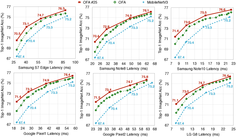
Figure 10 reports detailed comparisons between OFA and MobileNetV3 on six mobile devices. Remarkably, OFA can produce the entire trade-off curves with many points over a wide range of latency constraints by training only once (green curve). It is impossible for previous NAS methods (Tan et al., 2019; Cai et al., 2019) due to the prohibitive training cost.
OFA for Diverse Hardware Platforms.
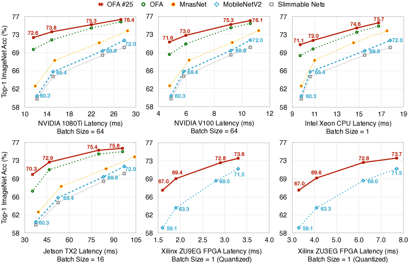
Besides the mobile platforms, we extensively studied the effectiveness of OFA on six additional hardware platforms (Figure 11) using the ProxylessNAS architecture space (Cai et al., 2019). OFA consistently improves the trade-off between accuracy and latency by a significant margin, especially on GPUs which have more parallelism. With similar latency as MobileNetV2 0.35, “OFA #25” improves the ImageNet top1 accuracy from MobileNetV2’s 60.3% to 72.6% (+12.3% improvement) on the 1080Ti GPU. Detailed architectures of our specialized models are shown in Figure 14. It reveals the insight that using the same model for different deployment scenarios with only the width multiplier modified has a limited impact on efficiency improvement: the accuracy drops quickly as the latency constraint gets tighter.

OFA for Specialized Hardware Accelerators.
There has been plenty of work on NAS for general-purpose hardware, but little work has been focused on specialized hardware accelerators. We quantitatively analyzed the performance of OFA on two FPGAs accelerators (ZU3EG and ZU9EG) using Xilinx Vitis AI with 8-bit quantization, and discuss two design principles.
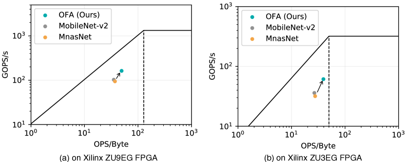
Principle 1: memory access is expensive, computation is cheap. An efficient CNN should do as much as computation with a small amount of memory footprint. The ratio is defined as the arithmetic intensity (OPs/Byte). The higher OPs/Byte, the less memory bounded, the easier to parallelize. Thanks to OFA’s diverse choices of sub-network architectures () (Section 3.3), and the OFA model twin that can quickly give the accuracy/latency feedback (Section 3.4), the evolutionary search can automatically find a CNN architecture that has higher arithmetic intensity. As shown in Figure 12, OFA’s arithmetic intensity is 48%/43% higher than MobileNetV2 and MnasNet (MobileNetV3 is not supported by Xilinx Vitis AI). Removing the memory bottleneck results in higher utilization and GOPS/s by 70%-90%, pushing the operation point to the upper-right in the roofline model (Williams et al., 2009), as shown in Figure 13. (70%-90% looks small in the log scale but that is significant).
Principle 2: the CNN architecture should be co-designed with the hardware accelerator’s cost model. The FPGA accelerator has a specialized depth-wise engine that is pipelined with the point-wise engine. The pipeline throughput is perfectly matched for 3x3 kernels. As a result, OFA’s searched model only has 3x3 kernel (Figure 14, a) on FPGA, despite 5x5 and 7x7 kernels are also in the search space. Additionally, large kernels sometimes cause “out of BRAM” error on FPGA, giving high cost. On Intel Xeon CPU, however, more than 50% operations are large kernels. Both FPGA and GPU models are wider than CPU, due to the large parallelism of the computation array.

|
| (a) 4.1ms latency on Xilinx ZU3EG (batch size = 1). |

|
| (b) 10.9ms latency on Intel Xeon CPU (batch size = 1). |

|
| (c) 14.9ms latency on NVIDIA 1080Ti (batch size = 64). |
5 Conclusion
We proposed Once-for-All (OFA), a new methodology that decouples model training from architecture search for efficient deep learning deployment under a large number of hardware platforms. Unlike previous approaches that design and train a neural network for each deployment scenario, we designed a once-for-all network that supports different architectural configurations, including elastic depth, width, kernel size, and resolution. It reduces the training cost (GPU hours, energy consumption, and emission) by orders of magnitude compared to conventional methods. To prevent sub-networks of different sizes from interference, we proposed a progressive shrinking algorithm that enables a large number of sub-network to achieve the same level of accuracy compared to training them independently. Experiments on a diverse range of hardware platforms and efficiency constraints demonstrated the effectiveness of our approach. OFA provides an automated ecosystem to efficiently design efficient neural networks with the hardware cost model in the loop.
Acknowledgments
We thank NSF Career Award #1943349, MIT-IBM Watson AI Lab, Google-Daydream Research Award, Samsung, Intel, Xilinx, SONY, AWS Machine Learning Research Award for supporting this research. We thank Samsung, Google and LG for donating mobile phones. We thank Shuang Wu and Lei Deng for drawing the Figure 2.
References
- Ashok et al. (2018) Anubhav Ashok, Nicholas Rhinehart, Fares Beainy, and Kris M Kitani. N2n learning: Network to network compression via policy gradient reinforcement learning. In ICLR, 2018.
- Cai et al. (2018a) Han Cai, Tianyao Chen, Weinan Zhang, Yong Yu, and Jun Wang. Efficient architecture search by network transformation. In AAAI, 2018a.
- Cai et al. (2018b) Han Cai, Jiacheng Yang, Weinan Zhang, Song Han, and Yong Yu. Path-level network transformation for efficient architecture search. In ICML, 2018b.
- Cai et al. (2019) Han Cai, Ligeng Zhu, and Song Han. ProxylessNAS: Direct neural architecture search on target task and hardware. In ICLR, 2019. URL https://arxiv.org/pdf/1812.00332.pdf.
- Cheung et al. (2019) Brian Cheung, Alex Terekhov, Yubei Chen, Pulkit Agrawal, and Bruno Olshausen. Superposition of many models into one. In NeurIPS, 2019.
- Courbariaux et al. (2015) Matthieu Courbariaux, Yoshua Bengio, and Jean-Pierre David. Binaryconnect: Training deep neural networks with binary weights during propagations. In NeurIPS, 2015.
- Deng et al. (2009) Jia Deng, Wei Dong, Richard Socher, Li-Jia Li, Kai Li, and Li Fei-Fei. Imagenet: A large-scale hierarchical image database. In CVPR, 2009.
- Guo et al. (2019) Zichao Guo, Xiangyu Zhang, Haoyuan Mu, Wen Heng, Zechun Liu, Yichen Wei, and Jian Sun. Single path one-shot neural architecture search with uniform sampling. arXiv preprint arXiv:1904.00420, 2019.
- Han et al. (2015) Song Han, Jeff Pool, John Tran, and William Dally. Learning both weights and connections for efficient neural network. In NeurIPS, 2015.
- Han et al. (2016) Song Han, Huizi Mao, and William J Dally. Deep compression: Compressing deep neural networks with pruning, trained quantization and huffman coding. In ICLR, 2016.
- Hao et al. (2019) Cong Hao, Xiaofan Zhang, Yuhong Li, Sitao Huang, Jinjun Xiong, Kyle Rupnow, Wen-mei Hwu, and Deming Chen. Fpga/dnn co-design: An efficient design methodology for 1ot intelligence on the edge. In 2019 56th ACM/IEEE Design Automation Conference (DAC), pp. 1–6. IEEE, 2019.
- He et al. (2016) Kaiming He, Xiangyu Zhang, Shaoqing Ren, and Jian Sun. Deep residual learning for image recognition. In CVPR, 2016.
- He et al. (2018) Yihui He, Ji Lin, Zhijian Liu, Hanrui Wang, Li-Jia Li, and Song Han. Amc: Automl for model compression and acceleration on mobile devices. In ECCV, 2018.
- Hinton et al. (2015) Geoffrey Hinton, Oriol Vinyals, and Jeff Dean. Distilling the knowledge in a neural network. arXiv preprint arXiv:1503.02531, 2015.
- Howard et al. (2019) Andrew Howard, Mark Sandler, Grace Chu, Liang-Chieh Chen, Bo Chen, Mingxing Tan, Weijun Wang, Yukun Zhu, Ruoming Pang, Vijay Vasudevan, et al. Searching for mobilenetv3. In ICCV 2019, 2019.
- Howard et al. (2017) Andrew G Howard, Menglong Zhu, Bo Chen, Dmitry Kalenichenko, Weijun Wang, Tobias Weyand, Marco Andreetto, and Hartwig Adam. Mobilenets: Efficient convolutional neural networks for mobile vision applications. arXiv preprint arXiv:1704.04861, 2017.
- Huang et al. (2017) Gao Huang, Zhuang Liu, Laurens Van Der Maaten, and Kilian Q Weinberger. Densely connected convolutional networks. In CVPR, 2017.
- Huang et al. (2018) Gao Huang, Danlu Chen, Tianhong Li, Felix Wu, Laurens van der Maaten, and Kilian Q Weinberger. Multi-scale dense networks for resource efficient image classification. In ICLR, 2018.
- Iandola et al. (2016) Forrest N Iandola, Song Han, Matthew W Moskewicz, Khalid Ashraf, William J Dally, and Kurt Keutzer. Squeezenet: Alexnet-level accuracy with 50x fewer parameters and¡ 0.5 mb model size. arXiv preprint arXiv:1602.07360, 2016.
- Jiang et al. (2019a) Weiwen Jiang, Lei Yang, Edwin Sha, Qingfeng Zhuge, Shouzhen Gu, Yiyu Shi, and Jingtong Hu. Hardware/software co-exploration of neural architectures. arXiv preprint arXiv:1907.04650, 2019a.
- Jiang et al. (2019b) Weiwen Jiang, Xinyi Zhang, Edwin H-M Sha, Lei Yang, Qingfeng Zhuge, Yiyu Shi, and Jingtong Hu. Accuracy vs. efficiency: Achieving both through fpga-implementation aware neural architecture search. In Proceedings of the 56th Annual Design Automation Conference 2019, pp. 1–6, 2019b.
- Kuen et al. (2018) Jason Kuen, Xiangfei Kong, Zhe Lin, Gang Wang, Jianxiong Yin, Simon See, and Yap-Peng Tan. Stochastic downsampling for cost-adjustable inference and improved regularization in convolutional networks. In CVPR, 2018.
- Lin et al. (2017) Ji Lin, Yongming Rao, Jiwen Lu, and Jie Zhou. Runtime neural pruning. In NeurIPS, 2017.
- Liu et al. (2018) Chenxi Liu, Barret Zoph, Maxim Neumann, Jonathon Shlens, Wei Hua, Li-Jia Li, Li Fei-Fei, Alan Yuille, Jonathan Huang, and Kevin Murphy. Progressive neural architecture search. In ECCV, 2018.
- Liu et al. (2019) Hanxiao Liu, Karen Simonyan, and Yiming Yang. Darts: Differentiable architecture search. In ICLR, 2019.
- Liu & Deng (2018) Lanlan Liu and Jia Deng. Dynamic deep neural networks: Optimizing accuracy-efficiency trade-offs by selective execution. In AAAI, 2018.
- Liu et al. (2017) Zhuang Liu, Jianguo Li, Zhiqiang Shen, Gao Huang, Shoumeng Yan, and Changshui Zhang. Learning efficient convolutional networks through network slimming. In ICCV, 2017.
- Loshchilov & Hutter (2016) Ilya Loshchilov and Frank Hutter. Sgdr: Stochastic gradient descent with warm restarts. arXiv preprint arXiv:1608.03983, 2016.
- Ma et al. (2018) Ningning Ma, Xiangyu Zhang, Hai-Tao Zheng, and Jian Sun. Shufflenet v2: Practical guidelines for efficient cnn architecture design. In ECCV, 2018.
- Real et al. (2019) Esteban Real, Alok Aggarwal, Yanping Huang, and Quoc V Le. Regularized evolution for image classifier architecture search. In AAAI, 2019.
- Sandler et al. (2018) Mark Sandler, Andrew Howard, Menglong Zhu, Andrey Zhmoginov, and Liang-Chieh Chen. Mobilenetv2: Inverted residuals and linear bottlenecks. In CVPR, 2018.
- Strubell et al. (2019) Emma Strubell, Ananya Ganesh, and Andrew McCallum. Energy and policy considerations for deep learning in nlp. In ACL, 2019.
- Tan et al. (2019) Mingxing Tan, Bo Chen, Ruoming Pang, Vijay Vasudevan, Mark Sandler, Andrew Howard, and Quoc V Le. Mnasnet: Platform-aware neural architecture search for mobile. In Proceedings of the IEEE Conference on Computer Vision and Pattern Recognition, pp. 2820–2828, 2019.
- Wang et al. (2018) Xin Wang, Fisher Yu, Zi-Yi Dou, Trevor Darrell, and Joseph E Gonzalez. Skipnet: Learning dynamic routing in convolutional networks. In ECCV, 2018.
- Williams et al. (2009) Samuel Williams, Andrew Waterman, and David Patterson. Roofline: An insightful visual performance model for floating-point programs and multicore architectures. Technical report, Lawrence Berkeley National Lab.(LBNL), Berkeley, CA (United States), 2009.
- Wu et al. (2019) Bichen Wu, Xiaoliang Dai, Peizhao Zhang, Yanghan Wang, Fei Sun, Yiming Wu, Yuandong Tian, Peter Vajda, Yangqing Jia, and Kurt Keutzer. Fbnet: Hardware-aware efficient convnet design via differentiable neural architecture search. In CVPR, 2019.
- Wu et al. (2018) Zuxuan Wu, Tushar Nagarajan, Abhishek Kumar, Steven Rennie, Larry S Davis, Kristen Grauman, and Rogerio Feris. Blockdrop: Dynamic inference paths in residual networks. In CVPR, 2018.
- Yu & Huang (2019a) Jiahui Yu and Thomas Huang. Autoslim: Towards one-shot architecture search for channel numbers. arXiv preprint arXiv:1903.11728, 2019a.
- Yu & Huang (2019b) Jiahui Yu and Thomas Huang. Universally slimmable networks and improved training techniques. In ICCV, 2019b.
- Yu et al. (2019) Jiahui Yu, Linjie Yang, Ning Xu, Jianchao Yang, and Thomas Huang. Slimmable neural networks. In ICLR, 2019.
- Zhang et al. (2018) Xiangyu Zhang, Xinyu Zhou, Mengxiao Lin, and Jian Sun. Shufflenet: An extremely efficient convolutional neural network for mobile devices. In CVPR, 2018.
- Zhu et al. (2017) Chenzhuo Zhu, Song Han, Huizi Mao, and William J Dally. Trained ternary quantization. In ICLR, 2017.
- Zoph & Le (2017) Barret Zoph and Quoc V Le. Neural architecture search with reinforcement learning. In ICLR, 2017.
- Zoph et al. (2018) Barret Zoph, Vijay Vasudevan, Jonathon Shlens, and Quoc V Le. Learning transferable architectures for scalable image recognition. In CVPR, 2018.
Appendix A Details of the Accuracy Predictor
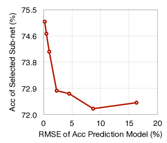
We use a three-layer feedforward neural network that has 400 hidden units in each layer as the accuracy predictor. Given a model, we encode each layer in the neural network into a one-hot vector based on its kernel size and expand ratio, and we assign zero vectors to layers that are skipped. Besides, we have an additional one-hot vector that represents the input image size. We concatenate these vectors into a large vector that represents the whole neural network architecture and input image size, which is then fed to the three-layer feedforward neural network to get the predicted accuracy. In our experiments, this simple accuracy prediction model can provide very accurate predictions. At convergence, the root-mean-square error (RMSE) between predicted accuracy and estimated accuracy on the test set is only 0.21%. Figure 15 shows the relationship between the RMSE of the accuracy prediction model and the final results (i.e., the accuracy of selected sub-networks). We can find that lower RMSE typically leads to better final results.
Appendix B Implementation Details of Progressive Shrinking
After training the full network, we first have one stage of fine-tuning to incorporate elastic kernel size. In this stage (i.e., ), we sample one sub-network in each update step. The network is fine-tuned for 125 epochs with an initial learning rate of 0.96. All other training settings are the same as training the full network.
Next, we have two stages of fine-tuning to incorporate elastic depth. We sample two sub-networks and aggregate their gradients in each update step. The first stage (i.e., ) takes 25 epochs with an initial learning rate of 0.08 while the second stage (i.e., ) takes 125 epochs with an initial learning rate of 0.24.
Finally, we have two stages of fine-tuning to incorporate elastic width. We sample four sub-networks and aggregate their gradients in each update step. The first stage (i.e., ) takes 25 epochs with an initial learning rate of 0.08 while the second stage (i.e., ) takes 125 epochs with an initial learning rate of 0.24.