Manifestations of Projection-Induced Memory: General Theory and the Tilted Single File

Abstract

Over the years the field of non-Markovian stochastic processes and anomalous diffusion evolved from a specialized topic to mainstream theory, which transgressed the realms of physics to chemistry, biology and ecology. Numerous phenomenological approaches emerged, which can more or less successfully reproduce or account for experimental observations in condensed matter, biological and/or single-particle systems. However, as far as their predictions are concerned these approaches are not unique, often build on conceptually orthogonal ideas, and are typically employed on an ad hoc basis. It therefore seems timely and desirable to establish a systematic, mathematically unifying and clean approach starting from more fine-grained principles. Here we analyze projection-induced ergodic non-Markovian dynamics, both reversible as well as irreversible, using spectral theory. We investigate dynamical correlations between histories of projected and latent observables that give rise to memory in projected dynamics, and rigorously establish conditions under which projected dynamics is Markovian or renewal. A systematic metric is proposed for quantifying the degree of non-Markovianity. As a simple, illustrative but non-trivial example we study single file diffusion in a tilted box, which, for the first time, we solve exactly using the coordinate Bethe ansatz. Our results provide a solid foundation for a deeper and more systematic analysis of projection-induced non-Markovian dynamics and anomalous diffusion.

1 Keywords:

Fokker-Planck equation, spectral theory, projection operator method, occupation time, single file diffusion, Bethe ansatz, free energy landscape

2 Introduction

Over the past decades the field of anomalous diffusion and non-Markovian dynamics grew to a mainstream physical topic [1, 2, 3, 4, 5, 6, 7, 8, 9, 10] backed up by a surge of experimental observations [11, 12, 13, 14, 15, 16] (the list of works is anything but exhaustive). From a theoretical point of view the description of anomalous and non-Markovian phenomena is not universal [1] and can be roughly (and judiciously) classified according to the underlying phenomenology: (i) renewal continuous-time random walk and fractional Fokker-Planck approaches [1, 2, 17, 3, 18], (ii) diffusion in disordered media [19, 20, 21, 22, 23, 24, 25, 26, 27], (iii) generalized Langevin equation descriptions [28, 29, 30, 31, 32, 33, 34, 35, 36], (iv) spatially heterogeneous diffusion [37, 38, 39, 40, 41, 42, 43], and more recently also (v) the so-called diffusing diffusivity models [44, 45, 46, 47, 48, 49, 50].

From a more general first-principles perspective non-Markovian dynamics in physical systems are always a result of the projection of nominally deterministic and/or Markovian high-dimensional dynamics to a lower-dimensional subspace [51, 52, 53, 54, 55, 56, 57, 58, 59, 60]. The projection in general induces a dependence of the dynamics on the initial conditions of the latent degrees of freedom, i.e. those being integrated out, thereby leading to memory [51, 54, 56, 55] and possibly (depending on the system) also to anomalous diffusion [61, 62, 63, 64, 65, 66, 67, 68].

Hallmarks of broken Markovianity are the non-validity of the Chapman-Kolmogorov equation, and on the level of individual trajectories correlations between histories of projected observables and latent degrees of freedom [67]. The advantage of such an approach is a deeper understanding and complete control over the origin and nature of memory effects. The drawback, however, is the inherent difficulty of integrating out exactly degrees of freedom in a microscopic model, such that in practice this seems to be only possible for the simplest models, e.g. harmonic systems (e.g. [69]), comb-models (e.g. [70, 71, 72]) or simple obstruction models [61, 62, 63, 64, 65, 66, 67], to name but a few.

Here, instead of focusing on the analysis of evolution equations for projected dynamics [51, 54, 56, 55] we focus on the consequences of the projection – both in a general setting as well as by means of a simplistic yet non-trivial model of single file diffusion in a tilted box. Using spectral theory we first present a rigorous and quite general analysis of the problem and establish conditions, under which the projection in fact leads to Markovian or renewal-type dynamics. We then apply these general results to the analysis of tagged particle diffusion in a single file confined in a tilted box. We obtain an exact solution of the full many-body and projected tagged particle propagators using the coordinate Bethe ansatz, and provide exact results for tagged particle local time statistics and correlations between tagged particle histories. Finally, to asses the degree of non-Markovianity induced by the projection, we compute the Kullback-Leibler divergence between the exact tagged particle propagator and the propagator of Markovian diffusion in the respective free energy landscape, i.e. in the so-called free energy landscape perspective. Our results provide a deeper understanding of projection-induced memory and anomalous diffusion and highlight important pitfalls in applications of free energy landscape-ideas in absence of a time-scale separation.

3 Theory

3.1 Notation and Mathematical Preliminaries

Although all presented result hold identically for discrete-state jump dynamics governed by a Markovian master equation we will throughout be interested in projections of continuous (in space as well as time) Markovian diffusion in a continuous domain $\Omega\in\mathbb{R}^{d}$ in a vector field $\mathbf{F}(\mathbf{x}):\mathbb{R}^{d}\to\mathbb{R}^{d}$ (not necessarily a potential field), which is either nominally confining (in this case $\Omega$ is open) or is accompanied by corresponding reflecting boundary conditions at $\partial\Omega$ (in this case $\Omega$ is closed) thus guaranteeing the existence of an invariant measure and hence ergodicity. The dynamics are governed by the (forward) Fokker-Planck operator $\hat{\mathcal{L}}:V\to V$ or its adjoint (or backward) operator $\hat{\mathcal{L}}^{\dagger}:W\to W$, where $V$ is a complete normed linear vector space with elements $f\in C^{2}(\mathbb{R}^{d})$ and $W$ is its dual space. In particular,

$$\hat{\mathcal{L}}=\nabla\cdot\mathbf{D}\nabla-\nabla\cdot\mathbf{F}(\mathbf{x}),\qquad\hat{\mathcal{L}}^{\dagger}=\nabla\cdot\mathbf{D}\nabla+\mathbf{F}(\mathbf{x})\cdot\nabla,$$ (1)

where $\mathbf{D}$ is the symmetric positive-definite diffusion matrix. $\hat{\mathcal{L}}$ propagates measures $\mu_{t}(\mathbf{x})$ in time, which will throughout be assumed to posses well-behaved probability density functions $P(\mathbf{x},t)$, i.e. $d\mu_{t}(\mathbf{x})=P(\mathbf{x},t)d\mathbf{x}$ (thereby posing some restrictions of $\mathbf{F}(\mathbf{x})$). Moreover, we assume that $\mathbf{F}(\mathbf{x})$ admits the following decomposition into a potential (irrotational) field $-\mathbf{D}\nabla\varphi(\mathbf{x})$ and a non-conservative component $\bm{\vartheta}(\mathbf{x})$, $\mathbf{F}(\mathbf{x})=-\mathbf{D}\nabla\varphi(\mathbf{x})+\bm{\vartheta}(\mathbf{x})$ with the two fields being mutually orthogonal $\nabla\varphi(\mathbf{x})\cdot\bm{\vartheta}(\mathbf{x})=0$ [73]. By insertion into Eq. (1) one can now easily check that $\hat{\mathcal{L}}\mathrm{e}^{-\varphi(\mathbf{x})}=0$, such that the steady-state solution of the Fokker-Planck equation by construction does not depend on the non-conservative part $\bm{\vartheta}(\mathbf{x})$. Before proceeding we first establish the decomposition of the drift field $\mathbf{F}(\mathbf{x})$ of the full dynamics, which with the knowledge of $\varphi(\mathbf{x})$ can be shown to have the form

$$\mathbf{F}(\mathbf{x})=-\mathbf{D}\nabla\varphi(\mathbf{x})+\mathrm{e}^{\varphi(\mathbf{x})}\mathbf{j}_{\text{ss}}(\mathbf{x}),$$ (2)

$\mathbf{j}_{\text{ss}}(\mathbf{x})$ denoting the steady-state probability current and $\bm{\vartheta}(\mathbf{x})\equiv\mathrm{e}^{\varphi(\mathbf{x})}\mathbf{j}_{\text{ss}}(\mathbf{x})$ being incompressible. The proof follows straightforwardly. We take $\bm{\vartheta}(\mathbf{x})=\mathbf{F}(\mathbf{x})+\mathbf{D}\nabla\varphi(\mathbf{x})$ and use $\varphi(\mathbf{x})$ to determine the steady-state current $\mathbf{j}_{\text{ss}}(\mathbf{x})=(\bm{\vartheta}(\mathbf{x})-\mathbf{D}\nabla\varphi(\mathbf{x}))\mathrm{e}^{-\varphi(\mathbf{x})}+\mathbf{D}\nabla\mathrm{e}^{-\varphi(\mathbf{x})}$, such that immediately $\bm{\vartheta}(\mathbf{x})=\mathrm{e}^{\varphi(\mathbf{x})}\mathbf{j}_{\text{ss}}(\mathbf{x})$ and in turn follows $\mathbf{F}(\mathbf{x})$ in Eq. (2). To check for incompressibility we note that $\mathbf{j}_{\text{ss}}(\mathbf{x})$ is by definition divergence free and so $\nabla\cdot\bm{\vartheta}(\mathbf{x})=\mathrm{e}^{\varphi(\mathbf{x})}(\mathbf{j}_{\text{ss}}(\mathbf{x})\cdot\nabla\varphi(\mathbf{x}))\equiv\bm{\vartheta}(\mathbf{x})\cdot\nabla\varphi(\mathbf{x})=0$, i.e. $\mathrm{e}^{\varphi(\mathbf{x})}\mathbf{j}_{\text{ss}}(\mathbf{x})$ is divergence-free, as claimed.

We define the forward and backward propagators by $\hat{U}(t)=\mathrm{e}^{\hat{\mathcal{L}}t}$ and $\hat{U}^{\dagger}(t)=\mathrm{e}^{\hat{\mathcal{L}}^{\dagger}t}$ such that $\hat{\mathcal{L}}$ and $\hat{\mathcal{L}}^{\dagger}$ are generators of a semi-group $\hat{U}(t+t^{\prime})=\hat{U}(t)\hat{U}(t^{\prime})$ and $\hat{U}^{\dagger}(t+t^{\prime})=\hat{U}^{\dagger}(t)\hat{U}^{\dagger}(t^{\prime})$, respectively. For convenience we introduce the bra-ket notation with the ’ket’ $|f\rangle$ representing a vector in $V$ (or $W$, respectively) written in position basis as $f(\mathbf{x})\equiv\langle\mathbf{x}|f\rangle$, and the ’bra’ $\langle g|$ as the integral $\int d\mathbf{x}g^{\dagger}$. The scalar product is defined as $\langle g|f\rangle=\int d\mathbf{x}g^{\dagger}(\mathbf{x})f(\mathbf{x})$. Therefore we have, in operator notation, the following evolution equation for the conditional probability density function starting from an initial condition $|p_{0}\rangle$: $|p_{t}\rangle=\mathrm{e}^{\hat{\mathcal{L}}t}|p_{0}\rangle$ and, since the process is ergodic, $\lim_{t\to\infty}\mathrm{e}^{\hat{\mathcal{L}}t}|p_{0}\rangle=|\mathrm{ss}\rangle$ defining the equilibrium or non-equilibrium steady state. In other words, $\hat{\mathcal{L}}|\mathrm{ss}\rangle=0$ and $\langle\mathrm{ss}|\hat{\mathcal{L}}^{\dagger}=0$, as a result of the duality. We also define the (typically non-normalizable) ’flat’ state $|\text{--}\rangle$, such that $\langle\mathbf{x}|\text{--}\rangle=1$ and $\langle\text{--}|p_{t}\rangle=1$. Hence, $\partial_{t}\langle\text{--}|p_{t}\rangle=0$ and $\langle\text{--}|\hat{\mathcal{L}}=0$ and $\hat{\mathcal{L}}^{\dagger}|\text{--}\rangle=0$. We define the Green’s function of the process as the conditional probability density function for a localized initial condition $\langle\mathbf{x}|p_{0}\rangle=\delta(\mathbf{x}-\mathbf{x}_{0})$ as

$$G(\mathbf{x},t|\mathbf{x}_{0},0)=\langle\mathbf{x}|\hat{U}(t)|\mathbf{x}_{0}\rangle\equiv\langle\mathbf{x}_{0}|\hat{U}^{\dagger}(t)|\mathbf{x}\rangle,$$ (3)

such that the conditional probability density starting from a general initial condition $|p_{0}\rangle$ becomes $P(\mathbf{x},t|p_{0},0)=\langle\mathbf{x}|\hat{U}(t)|p_{0}\rangle\equiv\int d\mathbf{x}_{0}p_{0}(\mathbf{x}_{0})G(\mathbf{x},t|\mathbf{x}_{0},0)$. Moreover, as $\mathbf{F}(\mathbf{x})$ is assumed to be sufficiently confining (i.e. $\lim_{\mathbf{x}\to\infty}P(\mathbf{x},t)=0,\forall t$ sufficiently fast), such that $\hat{\mathcal{L}}$ corresponds to a coercive and densely defined operator on $V$ (and $\hat{\mathcal{L}}^{\dagger}$ on $W$, respectively) [74, 75, 76]. Finally, $\hat{\mathcal{L}}$ is throughout assumed to be normal, i.e. $\hat{\mathcal{L}}^{\dagger}\hat{\mathcal{L}}-\hat{\mathcal{L}}\hat{\mathcal{L}}^{\dagger}=0$, where for reversible system (i.e. those obeying detailed balance) we have $\hat{\mathcal{L}}\hat{\mathcal{L}}^{\dagger}=\hat{\mathcal{L}}^{\dagger}\hat{\mathcal{L}}=0$. Because any normal compact operator is diagonalizable [77], we can expand $\hat{\mathcal{L}}$ (and $\hat{\mathcal{L}}^{\dagger}$) in a complete bi-orthonormal set of left $\langle\psi^{L}_{k}|$ and right $|\psi^{R}_{k}\rangle$ ($\langle\psi^{R}_{k}|$ and $|\psi^{L}_{k}\rangle$, respectively) eigenstates

$$\hat{\mathcal{L}}|\psi^{R}_{k}\rangle=-\lambda_{k}|\psi^{R}_{k}\rangle,\qquad\hat{\mathcal{L}}^{\dagger}|\psi^{L}_{k}\rangle=-\alpha_{k}|\psi^{L}_{k}\rangle,$$ (4)

with $\text{Re}(\lambda_{k})\geq 0$, and according to our definition of the scalar product we have

$$\langle\psi^{L}_{k}|\hat{\mathcal{L}}|\psi^{R}_{k}\rangle=-\lambda_{k}\langle\psi^{L}_{k}|\psi^{R}_{k}\rangle=\left(\langle\psi^{R}_{k}|\hat{\mathcal{L}}^{\dagger}|\psi^{L}_{k}\rangle\right)^{\dagger}=-\alpha_{k}^{\dagger}\langle\psi^{R}_{k}|\psi^{L}_{k}\rangle$$ (5)

and hence the spectra of $\hat{\mathcal{L}}$ and $\hat{\mathcal{L}}^{\dagger}$ are complex conjugates, $\alpha_{k}=\lambda_{k}^{\dagger}$. Moreover, $\lambda_{0}=0$, $|\psi^{R}_{0}\rangle=|\mathrm{ss}\rangle$, $\langle\psi^{L}_{0}|=\langle\text{--}|$, and $\langle\psi^{L}_{k}|\psi^{R}_{l}\rangle=\delta_{kl}$. Finally, we also have the resolution of identity $\mathbf{1}=\sum_{k}|\psi^{R}_{k}\rangle\langle\psi^{L}_{k}|$ and the propagator $\hat{U}(t)=\sum_{k}|\psi^{R}_{k}\rangle\langle\psi^{L}_{k}|\mathrm{e}^{-\lambda_{k}t}$. It follows that the spectral expansion of the Green’s function reads

$$G(\mathbf{x},t|\mathbf{x}_{0},0)=\sum_{k}\psi^{R}_{k}(\mathbf{x})\psi_{k}^{L\dagger}(\mathbf{x}_{0})\mathrm{e}^{-\lambda_{k}t}\equiv\sum_{k}\psi^{L}_{k}(\mathbf{x}_{0})\psi_{k}^{R\dagger}(\mathbf{x})\mathrm{e}^{-\lambda_{k}^{\dagger}t},$$ (6)

We now define, $\hat{\mathcal{P}}_{\mathbf{x}}(\bm{\Gamma};\mathbf{q})$, a (potentially oblique) projection operator into a subspace of random variables – a mapping $\mathbf{q}=\bm{\Gamma}(\mathbf{x}):\mathbb{R}^{d}\to\mathbb{R}^{a}$ to a subset of coordinates $\mathbf{q}$ lying in some orthogonal system in Euclidean space, $\mathbf{q}\in\Xi(\mathbb{R}^{a})\subset\Omega(\mathbb{R}^{d})$ with $a<d$. For example, the projection operator applied to some function $R(\mathbf{x})\in V$ gives

$$\hat{\mathcal{P}}_{\mathbf{x}}(\bm{\Gamma};\mathbf{q})R(\mathbf{x})=\int_{\Omega}d\mathbf{x}\delta(\bm{\Gamma}(\mathbf{x})-\mathbf{q})R(\mathbf{x}).$$ (7)

The spectral expansion of $\hat{\mathcal{L}}$ (and $\hat{\mathcal{L}}^{\dagger}$) in the bi-orthogonal Hilbert space alongside the projection operator $\hat{\mathcal{P}}_{\mathbf{x}}(\bm{\Gamma};\mathbf{q})$ will now allow us to define and analyze projection-induced non-Markovian dynamics.

3.2 General Results

3.2.1 Non-Markovian Dynamics and (non)Existence of a Semigroup

Using the projection operator $\hat{\mathcal{P}}_{\mathbf{x}}(\bm{\Gamma};\mathbf{q})$ defined in Eq. (7) we can define the (in general) non-Markovian Green’s function of the projected dynamics as the conditional probability density of projected dynamics starting from a localized initial condition $\mathbf{q}_{0}$

$$Q_{p_{0}}(\mathbf{q},t|\mathbf{q}_{0},0)=\frac{Q_{p_{0}}(\mathbf{q},t,\mathbf{q}_{0},0)_{p_{0}}}{Q_{p_{0}}^{0}(\mathbf{q}_{0})}\equiv\frac{\hat{\mathcal{P}}_{\mathbf{x}}(\Gamma;\mathbf{q})\hat{\mathcal{P}}_{\mathbf{x}_{0}}(\Gamma;\mathbf{q}_{0})G(\mathbf{x},t|\mathbf{x}_{0},0)p_{0}(\mathbf{x}_{0})}{\hat{\mathcal{P}}_{\mathbf{x}_{0}}(\Gamma;\mathbf{q}_{0})p_{0}(\mathbf{x}_{0})},$$ (8)

which demonstrates that the time evolution of projected dynamics starting from a fixed condition $\mathbf{q}_{0}$ depends on the initial preparation of the full system $p_{0}(\mathbf{x}_{0})$ as denoted by the subscript. This is a first signature of the non-Markovian and non-stationary nature of projected dynamics and was noted upon also in [55]. Obviously, $\int_{\Xi}d\mathbf{q}Q_{p_{0}}(\mathbf{q},t|\mathbf{q}_{0},0)=1$ for any initial condition $\mathbf{q}_{0}$. We will refer to $\mathbf{q}$ as the projected degrees of freedom, whereas those integrated out will be called latent. For the sake of simplicity we will here mostly limit our discussion to a stationary preparation of the system, i.e. $p_{0}(\mathbf{x}_{0})=p_{\text{ss}}(\mathbf{x}_{0})=\langle\mathbf{x}_{0}|\mathrm{ss}\rangle$. In order to avoid duplicating results we will explicitly carry out the calculation with the spectral expansion of $\hat{\mathcal{L}}$ but note that equivalent results are obtained using $\hat{\mathcal{L}}^{\dagger}$. Using the spectral expansion Eq. (6) and introducing $\Psi_{kl}(\mathbf{q})$, the elements of an infinite-dimensional matrix

$$\Psi_{kl}(\mathbf{q})=\langle\psi^{L}_{k}|\delta(\bm{\Gamma}(\mathbf{x})-\mathbf{q})|\psi^{R}_{l}\rangle$$ (9)

we find from Eq. (8)

$$Q_{p_{\text{ss}}}(\mathbf{q},t|\mathbf{q}_{0},0)=\sum_{k}\Psi_{0k}(\mathbf{q})(\Psi_{k0}(\mathbf{q}_{0})/\Psi_{00}(\mathbf{q}_{0}))\mathrm{e}^{-\lambda_{k}t}$$ (10)

with $\Psi_{00}(\mathbf{q}_{0})=Q_{p_{\text{ss}}}^{0}(\mathbf{q}_{0})$. If one would to identify $\Psi_{0k}(\mathbf{q})=\Psi^{R}_{0k}(\mathbf{q})$ and $\Psi_{00}(\mathbf{q}_{0})^{-1}\Psi_{0k}(\mathbf{q})=\Psi^{L}_{0k}(\mathbf{q})$, Eq. (10) at first sight looks deceivingly similar to the Markovian Green’s function in Eq. (6). Moreover, a hallmark of Markovian dynamics is that it obeys the Chapman-Kolmogorov equation and indeed, since $\langle\psi^{L}_{k}|\psi^{R}_{l}\rangle=\delta_{kl}$, we find from the spectral expansion Eq. (6) directly for any $0<t^{\prime}<t$ that

$$\int_{\Omega}d\mathbf{x}^{\prime}G(\mathbf{x},t|\mathbf{x}^{\prime},t^{\prime})G(\mathbf{x}^{\prime},t^{\prime}|\mathbf{x}_{0},0)=\sum_{k,l}\psi^{R}_{k}(\mathbf{x})\langle\psi^{L}_{k}|\psi^{R}_{l}\rangle\psi^{L\dagger}_{l}(\mathbf{x}_{0})\mathrm{e}^{-\lambda_{k}(t-t^{\prime})-\lambda_{l}t^{\prime}}\equiv G(\mathbf{x},t|\mathbf{x}_{0},0).$$ (11)

For non-Markovian dynamics with a stationary $p_{0}(\mathbf{x})$ it is straightforward to prove the following

Proposition 1: Let the full system be prepared in a steady state, $p_{0}(\mathbf{x})=p_{\mathrm{ss}}(\mathbf{x})$, and let non-Markovian Green’s function be defined by Eq. (8). We take $\Psi_{kl}(\mathbf{q})$ as defined in Eq. (9) and define a scalar product with respect to a Lebesgue measure $w$ as $\langle f|g\rangle_{w}\equiv\int d\mathbf{x}w(\mathbf{x})f^{\dagger}(\mathbf{x})g(\mathbf{x})$. Then Green’s function of the projected process will obey the Chapman-Kolmogorov equation if and only if $\langle\Psi_{l0}|\Psi_{k0}\rangle_{\Psi_{00}^{-1}}=0,\forall k,l$.

We need to prove if and under which conditions

$$\int_{\Xi}d\mathbf{q}^{\prime}Q_{p_{\text{ss}}}(\mathbf{q},t|\mathbf{q}^{\prime},t^{\prime})Q_{p_{\text{ss}}}(\mathbf{q}^{\prime},t^{\prime}|\mathbf{q}_{0},0)$$ (12)

can be equal to $Q_{p_{\text{ss}}}(\mathbf{q},t|\mathbf{q}_{0},0)$. As this will generally not be the case this essentially means that the projected dynamics is in general non-Markovian. The proof is established by noticing that $\Psi_{kl}(\mathbf{q}^{\prime})=\Psi_{lk}^{\dagger}(\mathbf{q}^{\prime})$ such that $\langle\Psi_{l0}|\Psi_{k0}\rangle_{\Psi_{00}^{-1}}\equiv\int_{\Xi}d\mathbf{q}^{\prime}\Psi_{00}(\mathbf{q}^{\prime})^{-1}\Psi_{0l}(\mathbf{q}^{\prime})\Psi_{k0}(\mathbf{q}^{\prime})$ $\Psi_{00}(\mathbf{q})^{-1}d\mathbf{q}$. As a result Eq. (12) can be written analogously to the first equality in Eq. (11) as

$$\sum_{k,l}\Psi_{0k}(\mathbf{q})\langle\Psi_{l0}|\Psi_{k0}\rangle_{\Psi_{00}^{-1}}(\Psi_{0l}^{\dagger}(\mathbf{q}_{0})/\Psi_{00}(\mathbf{q}_{0}))\mathrm{e}^{-\lambda_{k}(t-t^{\prime})-\lambda_{l}t^{\prime}}.$$ (13)

But since the projection mixes all excited eigenstates with $k>0$ (to a $k$-dependent extent) with the left and right ground states (see Eq. (9)), the orthogonality between $\Psi_{00}(\mathbf{q})^{-1/2}\Psi_{0l}(\mathbf{q})$ and $\Psi_{00}(\mathbf{q})^{-1/2}\Psi_{k0}(\mathbf{q})$ is in general lost, and $\langle\Psi_{l0}|\Psi_{k0}\rangle_{\Psi_{00}^{-1}}\neq 0$ for $k\neq l$ as claimed above. The Chapman-Kolmogorov equation can hence be satisfied if and only if $\langle\Psi_{l0}|\Psi_{k0}\rangle_{\Psi_{00}^{-1}}=0$ for all $k\neq l$. $\blacksquare$

However, even if $\langle\Psi_{l0}|\Psi_{k0}\rangle_{\Psi_{00}^{-1}}=0,\forall k\neq l$ this does not guarantee that the projected process is actually Markovian (see [78, 79] for observations made in the consideration of specific model examples). The computation of higher-order probability densities is necessary in order to check for Markovianity.

3.2.2 When is the Projected Dynamics Markovian or Renewal?

A) Projected Dynamics is Markovian

A particularly useful aspect of the present spectral-theoretic approach is its ability to establish rigorous conditions for the emergence of (exactly) Markovian and (exactly) renewal-type dynamics from a microscopic, first principles point of view. Note that in this section we assume a general, non-stationary preparation of the system (i.e. $p_{0}(\mathbf{x}_{0})\neq p_{\text{ss}}(\mathbf{x}_{0})$). By inspection of Eqs. (9) and (10) one can establish that:

Theorem 2: The necessary and sufficient condition for the projected dynamics to be Markovian if is that the projection $\hat{\mathcal{P}}_{\mathbf{\mathbf{x}}}(\bm{\Gamma};\mathbf{q})$ (whatever its form) nominally projects into the nullspace of latent dynamics. In other words, the latent and projected dynamics remain decoupled and orthogonal for all times. This means that (i) there exists a bijective map $\mathbf{y}=f(\mathbf{x})$ to a decomposable coordinate system $\mathbf{y}=(\mathbf{q},\mathbf{q}^{\prime\prime})$, in which the forward generator decomposes to $\hat{\mathcal{L}}=\hat{\mathcal{L}}_{p}+\hat{\mathcal{L}}_{l}$, where $\hat{\mathcal{L}}_{p}$ only acts and depends on the projected degrees of freedom $\mathbf{q}\in\Xi(\mathbb{R}^{a})\subset\Omega(\mathbb{R}^{d})$ with $a<d$ and $\hat{\mathcal{L}}_{l}$ only acts and depends on the latent coordinates $\mathbf{q}^{\prime\prime}\in\Xi^{c}(\mathbb{R}^{d})\subset\Omega(\mathbb{R}^{d})$ (with , $\Xi\cap\Xi^{\prime\prime}=\emptyset$, $\Omega=\Xi\cup\Xi^{\prime\prime}$), (ii) the boundary conditions on $\partial\Xi$ and $\partial\Xi^{c}$ are decoupled, and (iii) the projection operator $\hat{\mathcal{P}}_{\mathbf{\mathbf{y}}}(\cdot;\mathbf{q})=\int d\mathbf{q}^{\prime\prime}$ onto the subset of coordinates $\mathbf{q}\in\Xi(\mathbb{R}^{a})\subset\Omega$ corresponds to an integral over the subset of latent coordinates $\mathbf{q}^{\prime\prime}\in\Xi^{c}(\mathbb{R}^{d-a})\subset\Omega$, which does not mix projected and latent degrees of freedom, or alternatively $\hat{\mathcal{L}}_{l}p_{0}(\mathbf{q}_{0},\mathbf{q}_{0}^{\prime\prime})=0$.

The proof is rather straightforward and follows from the fact that if (and only if) the projected dynamics is Markovian it must be governed as well by a formal (Markovian) Fokker-Planck generator $\hat{\mathcal{L}}_{p}$ as in Eq. (1), in which the projected and latent degrees of freedom are separable $\hat{\mathcal{L}}=\hat{\mathcal{L}}_{p}+\hat{\mathcal{L}}_{l}$, and that the full Hilbert space is a direct sum of Hilbert spaces of the $V=V_{p}\oplus V_{l}$, that is $\hat{\mathcal{L}}:V\to V$, $\hat{\mathcal{L}}_{p}:V_{p}\to V_{p}$ and $\hat{\mathcal{L}}_{l}:V_{l}\to V_{l}$ and $V_{p}\cap V_{l}=\emptyset$. This also requires that there is no boundary condition coupling vectors from $V_{p}$ and $V_{l}$. In turn this implies assertion (i) above. If $\hat{\mathcal{P}}_{\mathbf{y}}(\cdot;\mathbf{q})$ is such that it does not mix eigenfunctions in $V_{p}$ and $V_{l}$ (i.e. it only involves vectors from $V_{p}$) then because of bi-orthonormality and the fact that $\langle\text{--}|\hat{\mathcal{L}}=0$ the projected Green’s function in full space $Q(\mathbf{q},t|\mathbf{q}_{0})$ for $\mathbf{q}\in\Xi(\mathbb{R}^{a})$ will be identical to the full Green’s function in the isolated domain $G(\mathbf{x},t|\mathbf{x}_{0})$ for $\mathbf{x}\in\Xi(\mathbb{R}^{a})$ and the non-mixing condition is satisfied. The effect is the same if the latent degrees of freedom already start in a steady state, $\hat{\mathcal{L}}_{l}p_{0}(\mathbf{q}_{0},\mathbf{q}_{0}^{\prime\prime})=0$. This establishes sufficiency. However, as soon as the projection mixes the two Hilbert spaces $V_{p}$ and $V_{l}$, the generator of projected dynamics will pick up contributions from $\hat{\mathcal{L}}_{l}$ and will, upon integrating out the latent degrees of freedom, not be Markovian. This completes the proof. $\blacksquare$

B) Projected Dynamics is Renewal

We can also rigorously establish sufficient conditions for the projected dynamics to poses the renewal property. Namely, the physical notion of a waiting time or a random change of time-scale (see, e.g. [2, 3]) can as well be attributed a microscopic origin. The idea of a random waiting time (or a random change of time scale) nominally implies a period of time and thereby the existence of some sub-domain, during which and within the latent degrees evolve while the projected dynamics does not change. For this to be the case the latent degrees of freedom must be perfectly orthogonal to the projected degrees of freedom, both in the two domains as well as on their boundaries (a prominent simple example is the so-called comb model [70, 71, 72]). Moreover, the projected degrees of freedom evolve only when the latent degrees of freedom reside in some subdomain $\Upsilon\subset\Xi^{c}(\mathbb{R}^{d-a})$. In turn, this means that the dynamics until a time $t$ ideally partitions between projected and latent degrees of freedom, which are coupled solely by the fact that the total time spent in each must add to $t$, which effects the waiting time. In a comb-setting the motion along the backbone occurs only when the particle is in the center of the orthogonal plane. In the context of a low-dimensional projection of ergodic Markovian dynamics, we can in fact prove the following general theorem:

Theorem 3: Let there exists a bijective map $\mathbf{y}=f(\mathbf{x})$ to a decomposable coordinate system $\mathbf{y}=(\mathbf{q},\mathbf{q}^{\prime\prime})$ as in A) with the projected $\mathbf{q}\in\Xi(\mathbb{R}^{a})$ and latent degrees of freedom $\mathbf{q}^{\prime\prime}\in\Xi^{c}(\mathbb{R}^{d-a})\equiv\Omega(\mathbb{R}^{d})\setminus\Xi(\mathbb{R}^{a})$. Furthermore, let $\Upsilon\subset\Xi^{c}(\mathbb{R}^{d-a})$ and let $\mathbbm{1}_{\Upsilon}(\mathbf{q}^{\prime\prime})$ denote the indicator function of the region $\Upsilon$ (i.e. $\mathbbm{1}_{\Upsilon}(\mathbf{q}^{\prime\prime})=1$ if $\mathbf{q}^{\prime\prime}\in\Upsilon$ and zero otherwise). Moreover, let the full system be prepared in an initial condition $p_{0}(\mathbf{q},\mathbf{q}^{\prime\prime})$. Then a sufficient condition for renewal-type dynamics is (i) that the forward generator in $(\mathbf{q},\mathbf{q}^{\prime\prime})$ decomposes $\hat{\mathcal{L}}=\mathbbm{1}_{\Upsilon}(\mathbf{q}^{\prime\prime})\hat{\mathcal{L}}_{p}+\hat{\mathcal{L}}_{l}$, and where $\hat{\mathcal{L}}_{p}$ only acts and depends on $\mathbf{q}$ and $\hat{\mathcal{L}}_{l}$ only acts and depends on $\mathbf{q}^{\prime\prime}$, and (ii) the boundary conditions do not cause a coupling of latent and projected degrees of freedom (as in the Markov case above).

The proof can be established by an explicit construction of the exact evolution equation for the projected variables. Let $G_{l}(\mathbf{q}^{\prime\prime},t|\mathbf{q}^{\prime\prime}_{0})$ denote the Green’s functions of the Markovian problem for the latent degrees of freedom, $G_{l}(\mathbf{q}^{\prime\prime},t|\mathbf{q}^{\prime\prime}_{0})=\langle\mathbf{q}^{\prime\prime}|\mathrm{e}^{\hat{\mathcal{L}}_{l}t}|\mathbf{q}^{\prime\prime}_{0}\rangle=\sum_{k}\langle\mathbf{q}^{\prime\prime}|\psi^{l,R}_{k}\rangle\langle\psi^{l,L}_{k}|\mathbf{q}_{0}^{\prime\prime}\rangle\mathrm{e}^{-\lambda_{k}^{l}t}$ and let $\tilde{g}(s)=\int_{0}^{\infty}\mathrm{e}^{-st}g(t)dt$ denoted the Laplace transform of a function $g(t)$. The projection operator in this case corresponds to $\hat{\mathcal{P}}_{\mathbf{q}^{\prime\prime}}(\cdot;\mathbf{q})=\int_{\Xi^{c}}d\mathbf{q}^{\prime\prime}$. We introduce the shorthand notation $\overline{p}_{0}(\mathbf{q})=\int_{\Xi^{c}}d\mathbf{q}_{0}^{\prime\prime}p_{0}(\mathbf{q}_{0},\mathbf{q}_{0}^{\prime\prime})$ and define the conditional initial probability density $p_{0}(\mathbf{q}_{0}^{\prime\prime}|\mathbf{q}_{0})=p_{0}(\mathbf{q}_{0},\mathbf{q}_{0}^{\prime\prime})/\overline{p}_{0}(\mathbf{q}_{0})$. The Green’s function of projected dynamics becomes $Q_{p_{0}}(\mathbf{q},t|\mathbf{q}_{0})=\int_{\Xi^{c}}d\mathbf{q}^{\prime\prime}\int_{\Xi^{c}}d\mathbf{q}_{0}^{\prime\prime}G(\mathbf{q},\mathbf{q}^{\prime\prime},t|\mathbf{q}_{0},\mathbf{q}^{\prime\prime}_{0})p_{0}(\mathbf{q}_{0},\mathbf{q}^{\prime\prime}_{0})/\overline{p}_{0}(\mathbf{q}_{0})$. We then have the following lemma:

Lemma 4: Under the specified assumptions $Q(\mathbf{q},t|\mathbf{q}_{0})$ exactly obeys the renewal-type non-Markovian Fokker-Planck equation

$$\partial_{t}Q_{p_{0}}(\mathbf{q},t|\mathbf{q}_{0})=\int_{0}^{t}d\tau K_{p_{0}}(t-\tau)\hat{\mathcal{L}}_{p}Q_{p_{0}}(\mathbf{q},\tau|\mathbf{q}_{0}),$$ (14)

with the memory kernel

$$K_{p_{0}}(t) = (\delta(t)+\partial_{t})\int_{\Upsilon}d\mathbf{q}^{\prime\prime}\int_{\Xi^{c}}d\mathbf{q}^{\prime\prime}_{0}p_{0}(\mathbf{q}_{0}^{\prime\prime}|\mathbf{q}_{0})\langle\mathbf{q}^{\prime\prime}|\mathrm{e}^{\hat{\mathcal{L}}_{l}t}|\mathbf{q}^{\prime\prime}_{0}\rangle$$ (15)

$$= \sum_{k}\left(\int_{\Xi^{c}}d\mathbf{q}_{0}^{\prime\prime}\psi^{l,L\dagger}_{k}(\mathbf{q}^{\prime\prime}_{0})p_{0}(\mathbf{q}_{0}^{\prime\prime}|\mathbf{q}_{0})\right)\left(\int_{\Upsilon}d\mathbf{q}^{\prime\prime}\psi^{l,R}_{k}(\mathbf{q}^{\prime\prime})\right)(\delta(t)-\lambda_{k}^{l}\mathrm{e}^{-\lambda_{k}^{l}t})$$

that is independent of $\mathbf{q}$ . Moreover, $Q(\mathbf{q},t|\mathbf{q}_{0})>0$ for all $t>0$ and for all $\mathbf{q},\mathbf{q}_{0}\in\Xi$.

To prove the lemma we Laplace transform equation ($t\to u$) $\partial_{t}G(\mathbf{q},\mathbf{q}^{\prime\prime},t|\mathbf{q}_{0},\mathbf{q}^{\prime\prime}_{0})=\hat{\mathcal{L}}G(\mathbf{q},\mathbf{q}^{\prime\prime},t|\mathbf{q}_{0},\mathbf{q}^{\prime\prime}_{0})$ and realize that the structure of $\hat{\mathcal{L}}$ implies that its solution with initial condition $\delta(\mathbf{q}-\mathbf{q}_{0})\delta(\mathbf{q}^{\prime\prime}-\mathbf{q}^{\prime\prime}_{0})$ in Laplace space factorizes $\tilde{G}(\mathbf{q},\mathbf{q}^{\prime\prime},u|\mathbf{q}_{0},\mathbf{q}^{\prime\prime}_{0})=f_{u}(\mathbf{q}|\mathbf{q}_{0})g_{u}(\mathbf{q}^{\prime\prime}|\mathbf{q}_{0}^{\prime\prime})$ with $g_{u}$ and $f_{u}$ to be determined. Note that $\int_{\Xi}d\mathbf{q}\int_{\Xi^{c}}d\mathbf{q}^{\prime\prime}\tilde{G}(\mathbf{q},\mathbf{q}^{\prime\prime},u|\mathbf{q}_{0},\mathbf{q}^{\prime\prime}_{0})=\int_{\Xi}d\mathbf{q}f_{u}(\mathbf{q}|\mathbf{q}_{0})\int_{\Xi^{c}}d\mathbf{q}^{\prime\prime}g_{u}(\mathbf{q}^{\prime\prime}|\mathbf{q}_{0}^{\prime\prime})=u^{-1}$ and we can chose, without any loss of generality that $\int_{\Xi}d\mathbf{q}f_{u}(\mathbf{q}|\mathbf{q}_{0})=1$. Plugging in the factorized ansatz and rearranging leads to

$$g_{u}(\mathbf{q}^{\prime\prime}|\mathbf{q}^{\prime\prime}_{0})\left(uf_{u}(\mathbf{q}|\mathbf{q}_{0})-\mathbbm{1}_{\Upsilon}(\mathbf{q}^{\prime\prime})\hat{\mathcal{L}}_{p}f_{u}(\mathbf{q}|\mathbf{q}_{0})\right)-f_{u}(\mathbf{q}|\mathbf{q}_{0})\hat{\mathcal{L}}_{l}g_{u}(\mathbf{q}^{\prime\prime}|\mathbf{q}^{\prime\prime}_{0})-\delta(\mathbf{q}-\mathbf{q}_{0})\delta(\mathbf{q}^{\prime\prime}-\mathbf{q}_{0}^{\prime\prime})=0.$$ (16)

Noticing that $\int_{\Xi}d\mathbf{q}\hat{\mathcal{L}}_{p}f(\mathbf{q}|\mathbf{q}_{0})=0$ as a result of the divergence theorem (as we assumed that $\mathbf{F}(\mathbf{x})$ is strongly confining implying that the current vanishes at the boundaries) we obtain, upon integrating Eq. (16) over $\mathbf{q}$

$$ug_{u}(\mathbf{q}^{\prime\prime}|\mathbf{q}^{\prime\prime}_{0})-\delta(\mathbf{q}^{\prime\prime}-\mathbf{q}_{0}^{\prime\prime})-\hat{\mathcal{L}}_{l}g_{u}(\mathbf{q}^{\prime\prime}|\mathbf{q}^{\prime\prime}_{0})=0,$$ (17)

implying that $g_{u}(\mathbf{q}^{\prime\prime}|\mathbf{q}_{0}^{\prime\prime})=\tilde{G}_{l}(\mathbf{q}^{\prime\prime},u|\mathbf{q}_{0}^{\prime\prime})$. As $\tilde{G}_{l}(\mathbf{q}^{\prime\prime},u|\mathbf{q}_{0}^{\prime\prime})$ is the Laplace image of a Markovian Green’s function we use $\int_{\Xi^{c}}d\mathbf{q}^{\prime\prime}\tilde{G}_{l}(\mathbf{q}^{\prime\prime},u|\mathbf{q}_{0}^{\prime\prime})=u^{-1}$ in order to deduce that $\tilde{Q}_{p_{0}}(\mathbf{q},u|\mathbf{q}_{0})=f_{u}(\mathbf{q}|\mathbf{q}_{0})/u$. The final step involves using the identified functions $f_{u}$ and $g_{u}$ in Eq. (16), multiplying with $p_{0}(\mathbf{q}_{0}^{\prime\prime}|\mathbf{q}_{0})$, integrating over $\mathbf{q}^{\prime\prime}$ and $\mathbf{q}_{0}^{\prime\prime}$ while using the divergence theorem implying $\int_{\Xi^{c}}d\mathbf{q}^{\prime\prime}\hat{\mathcal{L}}_{l}\tilde{G}_{l}(\mathbf{q}^{\prime\prime},u|\mathbf{q}_{0}^{\prime\prime})=0$ (as before) to obtain

$$u\tilde{Q}_{p_{0}}(\mathbf{q},u|\mathbf{q}_{0})-\delta(\mathbf{q}-\mathbf{q}_{0})=\left(u\int_{\Upsilon}d\mathbf{q}^{\prime\prime}\int_{\Xi^{c}}d\mathbf{q}_{0}^{\prime\prime}\tilde{G}_{l}(\mathbf{q}^{\prime\prime},u|\mathbf{q}_{0}^{\prime\prime})p_{0}(\mathbf{q}_{0}^{\prime\prime}|\mathbf{q}_{0})\right)\hat{\mathcal{L}}_{p}\tilde{Q}_{p_{0}}(\mathbf{q},u|\mathbf{q}_{0}).$$ (18)

Finally, since the Laplace transform of $\partial_{t}g(t)+\delta(t)g(0)$ corresponds to $u\tilde{g}(u)$, taking the inverse Laplace transform of Eq. (18) finally leads to Eqs. (14) and 15) and completes the proof of the lemma, since now we can take $Q_{p_{0}}(\mathbf{q},t|\mathbf{q}_{0})>0$ by definition because Eq. (14) is an identity of Eq. (1) integrated over $\mathbf{q}^{\prime\prime}$. Moreover, the rate of change of the Green’s function $Q_{p_{0}}(\mathbf{q},t|\mathbf{q}_{0})$ in Eq. (14) depends, at any instance $t$, position $\mathbf{q}$ and for any initial condition $\mathbf{q}_{0}$ only on the current position $\mathbf{q}$ and a waiting time (or random time-change) encoded in the memory kernel $K(t)$; $Q_{p_{0}}(\mathbf{q},t|\mathbf{q}_{0})$ is the Green’s function of a renewal process. This completes the proof of sufficiency. $\blacksquare$

Furthermore, for the situation where the full system is prepared in a stationary state, i.e. $p_{0}(\mathbf{x})=p_{\mathrm{s}}(\mathbf{x})$, we have the following corollary:

Corollary 5: Let the system and projection be defined as in Theorem 3. If the full system is prepared such that the latent degrees of freedom are in a stationary state $p_{0}(\mathbf{q}_{0},\mathbf{q}^{\prime\prime}_{0})$, such that $\hat{\mathcal{L}}_{l}p_{0}(\mathbf{q}^{\prime\prime}_{0}|\mathbf{q}_{0})=0,\forall\mathbf{q}_{0}\in\Xi$ and hence also $\overline{p}_{0}(\mathbf{q}_{0}^{\prime\prime})=\overline{p}_{\mathrm{ss}}(\mathbf{q}_{0}^{\prime\prime})$, then $p_{0}(\mathbf{q}^{\prime\prime}_{0}|\mathbf{q}_{0})=\psi^{l,R}_{0}(\mathbf{q}^{\prime\prime}_{0})$ and consequently $K_{p_{0}}=\delta(t)\int_{\Upsilon}d\mathbf{q}_{0}^{\prime\prime}\overline{p}_{\mathrm{ss}}(\mathbf{q}_{0}^{\prime\prime})$, and therefore the projected dynamics is Markovian. Moreover, if the system is prepared such that the latent degrees of freedom are not in a stationary state, i.e. $p_{0}(\mathbf{q}_{0}|\mathbf{q}^{\prime\prime}_{0})\neq\overline{p}_{\mathrm{ss}}(\mathbf{q}_{0}^{\prime\prime}),\forall\mathbf{q}_{0}$, there exists a finite time $t_{M}>0$ after which the dynamics will be arbitrarily close to being Markovian.

The proof of the first part follows from the bi-orthogonality of eigenfunctions of latent dynamics $\langle\psi^{l,R}_{k}|\psi^{l,R}_{0}\rangle=\delta_{k,0}$, rendering all terms in Eq. (15) in Lemma 4 identically zero except for $k=0$ with $\lambda_{k}^{l}=0$. The second part is established by the fact that for times $t_{M}\gg 1/\lambda_{1}^{l}$, with $\lambda_{1}^{l}$ being the largest (i.e. least negative) non-zero eigenvalue, all terms but the $k=0$ term in Eq. (15) in Lemma 4 become arbitrarily small. $\blacksquare$

Having established sufficiency, we now also comment on necessity of the conditions (i) and (ii) above for renewal dynamics. It is clear that the splitting of $\hat{\mathcal{L}}$ into $\hat{\mathcal{L}}_{p}$ and $\hat{\mathcal{L}}_{l}$, where $\hat{\mathcal{L}}_{l}$ does not act nor depend on projected variables, is also necessary condition for renewal. This can be established by contradiction as loosening these assumptions leads to dynamics that is not renewal. This can be understood intuitively, because it must hold that the latent degrees of freedom remain entirely decoupled from the projected ones (but not vice versa) and that the motion along both is mutually orthogonal. To illustrate this think of the paradigmatic comb model (see schematic in Fig.1) [70, 71, 72] and realize that renewal will be violated as soon as we tilt the side-branches for some angle from being orthogonal to the backbone.

Figure 1: Schematics of a generalized comb model. For the sake of clarity only a couple of side-branches are shown, whereas the model is to be understood in the sense of densely populated side-branches. (top) As long as the projected $q$ and latent $q^{\prime\prime}$ degree of freedom remain orthogonal, the projected dynamics will be of renewal-type. However, as soon as this ceases to be the case the projected dynamics will not be renewal.

However, since it is difficult to establish the most general class of admissible functions $h(\mathbf{q}^{\prime\prime})$ used in $\hat{\mathcal{L}}=h(\mathbf{q}^{\prime\prime})\hat{\mathcal{L}}_{p}+\hat{\mathcal{L}}_{l}$, we are not able to prove necessity. Based on the present analysis it seems somewhat difficult to systematically relax the assumptions for projected dynamics to be renewal without assuming, in addition, some sort of spatial discretization. We therefore hypothesize that the sufficient conditions stated in Theorem 3, potentially with some additional assumptions on $h(\mathbf{q}^{\prime\prime})$ are also necessary conditions. Notably, however, microscopic derivations of non-Markovian master equations of the form given in Eq. (14) often start in discretized space or ad hoc introduce a random change in time scale (see e.g. [2, 17, 80]).

3.2.3 Markovian Approximation and the Degree of non-Markovianity

In order to quantify the degree of non-Markovianity induced by the projection we propose to compare the full non-Markovian dynamics with projected dynamics evolving under a complete time-scale separation, i.e. under the assumption of all latent degrees of freedom being in the stationary state. To do so we proceed as follows. The projected coordinates $\mathbf{q}$ are now assumed to represent a subset of another $d$-dimensional orthogonal system in Euclidean space $\mathbf{q^{\prime}}\in\mathbb{R}^{d}$, and we assume the map $\mathbf{q}^{\prime}(\mathbf{x})$ is bijective. We denote the conditional probability density in this system by $G^{\prime}(\mathbf{q}^{\prime},t|\mathbf{q}^{\prime}_{0},0)$. The underlying physical idea is that an observer can only see the projected dynamics, which since it is non-Markovian stems from a projection but not necessarily onto Cartesian coordinates. Therefore, from a physical perspective not too much generality seems to be lost with this assumption.

As a concrete example one can consider the non-spherically symmetric Fokker-Planck process in a sphere, corresponding to the full Markovian parent system projected onto angular variables (either one or both). This way one first transforms from $\mathbf{x}\in\mathbb{R}^{3}$ to spherical coordinates $\mathbf{q}^{\prime}=(r,\phi,\theta)$ and then, e.g. projects on the the lines $\mathbf{q}=\phi\in[0,2\pi)$.

Since the transformation of the Fokker-Planck equation under a general change of coordinates is well-known [81] the task is actually simple. Under the complete map $\mathbf{q}^{\prime}=\bm{\Gamma}(\mathbf{x})$ with $\bm{\Gamma}:\mathbb{R}^{d}\to\mathbb{R}^{d}$ the forward Fokker-Planck operator in Eq. (1) transforms as $\hat{\mathcal{L}}^{\prime}=\nabla_{\mathbf{q}^{\prime}}\otimes\nabla_{\mathbf{q}^{\prime}}:\mathbf{\tilde{D}}(\mathbf{q}^{\prime})-\nabla_{\mathbf{q}^{\prime}}\cdot\mathbf{\tilde{F}}(\mathbf{q^{\prime}})$, where $\otimes$ and $:$ denote, respectively, the tensor and double-dot product, and the transformed drift field and diffusion tensor can be written as

$$(\mathbf{\tilde{F}}(\mathbf{q^{\prime}}))_{k}=\sum_{i=1}^{d}\frac{\partial q^{\prime}_{k}}{\partial x_{i}}\mathbf{F}_{i}+\sum_{i,j=1}^{d}D_{ij}\frac{\partial^{2}q_{k}}{\partial x_{i}\partial x_{j}},\quad(\mathbf{\tilde{D}}(\mathbf{q}^{\prime}))_{kl}=\sum_{i,j=1}^{d}D_{ij}\frac{\partial q^{\prime}_{k}}{\partial x_{i}}\frac{\partial q^{\prime}_{l}}{\partial x_{j}}.$$ (19)

We note that unless the mapping is linear, the old diffusion matrix affects the new drift vector and the diffusion matrix picks up a spatial dependence. For an excellent account of the transformation properties in the more general case of a position dependent diffusion matrix (i.e. $\mathbf{D}\to\mathbf{D}(\mathbf{x})$) we refer the reader to [82]. We now want to marginalize over the remaining (i.e. non-projected) coordinates $\mathbf{q}^{\prime\prime}\in\Omega\setminus\Xi$ but beforehand make the Markovian approximation $G^{\prime}(\mathbf{q}^{\prime},t|\mathbf{q}_{0},0)\approx Q_{M}(\mathbf{q},t|\mathbf{q}_{0})p_{\text{ss}}(\mathbf{q}^{\prime\prime})$. Then we have $\hat{\mathcal{L}}^{\prime}G^{\prime}(\mathbf{q}^{\prime},t|\mathbf{q}_{0},0)\approx p_{\text{ss}}(\mathbf{q}^{\prime\prime})\hat{\mathcal{L}}^{\prime}Q_{M}(\mathbf{q},t|\mathbf{q}_{0})$, implying that the operator $\hat{\mathcal{L}}^{\prime}$ approximately splits into one part operating on the projected coordinates alone, $\hat{\mathcal{L}}^{\prime}_{M}$, and one operating only on the latent stationary coordinates, $\hat{\mathcal{L}}^{\prime\prime}$, for which $\hat{\mathcal{L}}^{\prime\prime}p_{\text{ss}}(\mathbf{q}^{\prime\prime})=0$. The physical idea behind the Markovian approximation is that the latent degrees of freedom relax infinitely fast compared to the projected ones. Therefore, we can straightforwardly average the Fokker-Planck operator over the stationary latent coordinates $\mathbf{q}^{\prime\prime}$, $\langle\hat{\mathcal{L}}_{M}^{\prime}\rangle_{\mathbf{q}^{\prime\prime}}$, where we have defined the latent averaging operation $\langle\cdot\rangle_{\mathbf{q}^{\prime\prime}}\equiv\int d\mathbf{q}^{\prime\prime}p_{\text{ss}}(\mathbf{q}^{\prime\prime})\cdot$. Note that the remaining dependence of $\hat{\mathcal{L}}^{\prime}$ on the latent stationary coordinates $\mathbf{q}^{\prime\prime}$ is only due to $\mathbf{\tilde{F}}(\mathbf{q^{\prime}})$ and $\mathbf{\tilde{D}}(\mathbf{q}^{\prime})$. The averaged drift field and diffusion matrix now become

$$\langle\mathbf{\tilde{F}}(\mathbf{q})\rangle_{k}=\sum_{i=1}^{d}\left\langle\frac{\partial q^{\prime}_{k}}{\partial x_{i}}\mathbf{F}_{i}\right\rangle_{\mathbf{q}^{\prime\prime}}+\sum_{i,j=1}^{d}D_{ij}\left\langle\frac{\partial^{2}q_{k}}{\partial x_{i}\partial x_{j}}\right\rangle_{\mathbf{q}^{\prime\prime}},\quad\langle\mathbf{\tilde{D}}(\mathbf{q})\rangle_{kl}=\sum_{i,j=1}^{d}D_{ij}\left\langle\frac{\partial q^{\prime}_{k}}{\partial x_{i}}\frac{\partial q^{\prime}_{l}}{\partial x_{j}}\right\rangle_{\mathbf{q}^{\prime\prime}}.$$ (20)

We can further decompose the effective drift field into a conservative and a non-conservative part

$$\left\langle\frac{\partial q^{\prime}_{k}}{\partial x_{i}}\mathbf{F}_{i}\right\rangle_{\mathbf{q}^{\prime\prime}}=-\left\langle\frac{\partial q^{\prime}_{k}}{\partial x_{i}}\left(\mathbf{D}\nabla\varphi\right)_{i}\right\rangle_{\mathbf{q}^{\prime\prime}}+\left\langle\mathrm{e}^{\varphi}\frac{\partial q^{\prime}_{k}}{\partial x_{i}}(\mathbf{j}_{\text{ss}})_{i}\right\rangle_{\mathbf{q}^{\prime\prime}},$$ (21)

which establishes the Markovian approximation also for a broad class of irreversible systems. The approximate effective Fokker-Planck operator for the projected dynamics in turn reads

$$\langle\hat{\mathcal{L}}^{\prime}\rangle_{\mathbf{q}^{\prime\prime}}=\nabla_{\mathbf{q}}\otimes\nabla_{\mathbf{q}}:\langle\mathbf{\tilde{D}}(\mathbf{q})\rangle_{\mathbf{q}^{\prime\prime}}-\nabla_{\mathbf{q}}\cdot\langle\mathbf{\tilde{F}}(\mathbf{q})\rangle_{\mathbf{q}^{\prime\prime}}.$$ (22)

By design the kernel of $\langle\hat{\mathcal{L}}^{\prime}\rangle_{\mathbf{q}^{\prime\prime}}$ is equal to $p_{\text{ss}}(\mathbf{q})\equiv\hat{\mathcal{P}}_{\mathbf{x}}(\bm{\Gamma};\mathbf{q})p_{\text{ss}}(\mathbf{x})$, hence $\langle\hat{\mathcal{L}}^{\prime}\rangle_{\mathbf{q}^{\prime\prime}}$ governs the relaxation towards the steady-state density (not necessarily equilibrium) evolving from some initial state $\mathbf{q}_{0}$ in the Markovian approximation with the corresponding Green’s function $Q_{M}(\mathbf{q},t|\mathbf{q}_{0},0)\equiv\langle\mathbf{q}|\mathrm{e}^{\langle\hat{\mathcal{L}}^{\prime}\rangle_{\mathbf{q}^{\prime\prime}}t}|\mathbf{q}_{0}\rangle$.

In order to quantify the departure of the exact dynamics from the corresponding Markovian behavior we propose to evaluate the Kullback-Leibler divergence between the Green’s functions of the exact and Markovian propagator as a function of time

$$\mathcal{D}_{t}(Q||Q_{M})=\int_{\Xi}d\mathbf{q}Q(\mathbf{q},t|\mathbf{q}_{0},0)\ln\left(\frac{Q(\mathbf{q},t|\mathbf{q}_{0},0)}{Q_{M}(\mathbf{q},t|\mathbf{q}_{0},0)}\right).$$ (23)

By definition $\mathcal{D}_{t}(Q||Q_{M})\geq 0$ and since the non-Markovian behavior of the exact projected dynamics is transient with a life-time $\lambda_{1}^{-1}$, we have that $\lim_{t\to\infty}\mathcal{D}_{t}(Q||Q_{M})=0$. Our choice of quantifying the departure of the exact dynamics from the corresponding Markovian behavior is not unique. The Kullback-Leibler divergence introduced here can hence be used to quantify how fast the correlation of the latent degrees of freedom with the projected degrees of freedom dies out. Notably, in a related manner the Kullback-Leibler divergence was also used in the context of stochastic thermodynamics in order to disprove the hypothesis about the monotonicity of the entropy production as a general time evolution principle [83].

3.2.4 Functionals of Projected Dynamics

In order to gain deeper insight into the origin and manifestation of non-Markovian behavior it is instructive to focus on the statistics of time-average observables, that is functionals of projected dynamics. As in the previous sections we assume that the full system was prepared in a (potentially non-equilibrium current-carrying) steady state. To that end we have, using Feynman-Kac theory, recently proven a theorem connecting any bounded additive functional $\Phi_{t}[\mathbf{q}(\tau)]=t^{-1}\int_{0}^{t}Z(\mathbf{q}(\tau))d\tau$ (with a function $Z:\Xi(\mathbb{R}^{a})\to\mathbb{R}$ locally strictly bounded in $\Xi$) of projected dynamics $\mathbf{q}(\tau)$ of a parent Markovian diffusion $\mathbf{x}(t)$ to the eigenspectrum of the Markov generator of the full dynamics $\hat{\mathcal{L}}$ or $\hat{\mathcal{L}}^{\dagger}$ [67]. The central quantity of the theory is $\theta_{t}(\mathbf{s})$, the so-called local time fraction spent by a trajectory $\mathbf{q}(\tau)$ in a infinitesimal volume element $d\mathbf{s}$ centered at $\mathbf{s}$ up until a time $t$ enabling

$$\theta_{t}(\mathbf{s})=t^{-1}\int_{0}^{t}d\tau\mathbbm{1}_{\mathbf{s}}(\mathbf{q}(\tau))\quad\to\quad\Phi_{t}[\mathbf{q}(\tau)]=\int_{\Xi}d\mathbf{s}Z(\mathbf{s})\theta_{t}(\mathbf{s}),$$ (24)

where the indicator function $\mathbbm{1}_{\mathbf{s}}(\mathbf{q})=1$ if $\mathbf{q}=\mathbf{s}$ and zero otherwise. We are here interested in the fluctuations of $\theta_{t}(\mathbf{s})$ and correlation functions between the local time fraction of a projected observable $\mathbf{q}(t)$ at a point $\mathbf{s}$ and $\theta^{\prime\prime}(\mathbf{s}^{\prime})$, the local time some latent (hidden) observable $\mathbf{q}^{\prime\prime}(t)$ a the point $\mathbf{s}^{\prime}$:

$$\sigma^{2}_{t}(\mathbf{s})=\langle\theta^{2}_{t}(\mathbf{s})\rangle-\langle\theta_{t}(\mathbf{s})\rangle^{2},\quad\mathcal{C}_{t}(\mathbf{s};\mathbf{s}^{\prime})=\langle\theta_{t}(\mathbf{s})\theta^{\prime\prime}_{t}(\mathbf{s}^{\prime})\rangle-\langle\theta_{t}(\mathbf{s})\rangle\langle\theta^{\prime\prime}_{t}(\mathbf{s}^{\prime})\rangle,$$ (25)

where $\langle\cdot\rangle$ now denotes the average over all forward paths starting from the steady state $|\mathbf{q}_{0}\rangle=|\mathrm{ss}\rangle$ (and ending anywhere, i.e. $\langle\mathbf{q}|=\langle\text{--}|$), or, using the backward approach, all paths starting in the flat state $|\mathbf{q}\rangle=|\text{--}\rangle$ and propagating backward in time towards the steady state $\langle\mathbf{q}_{0}|=\langle\mathrm{ss}|$. We note that any correlation function of a general additive bounded functional $\Phi^{i}_{t}[\mathbf{q}(\tau)]$ of the form $\langle\Phi^{i}_{t}[\mathbf{q}(\tau)]\Phi^{j}_{t}[\mathbf{q}^{\prime\prime}(\tau)]\rangle$ (as well as the second moment of $\Phi^{i}_{t}[\mathbf{q}(\tau)]$) follows directly from the local time fraction, namely, $\langle\Phi^{i}_{t}[\mathbf{q}(\tau)]\Phi^{j}_{t}[\mathbf{q}^{\prime\prime}(\tau)]\rangle=\int_{\Xi}\int_{\Xi}d\mathbf{s}d\mathbf{s}^{\prime}Z_{i}(\mathbf{s})Z_{j}(\mathbf{s}^{\prime})\langle\theta_{t}(\mathbf{s})\theta^{\prime\prime}_{t}(\mathbf{s}^{\prime})\rangle$. For details of the theory and corresponding proofs please see [67], here we will simply state the main theorem:

Let the Green’s function of the full parent dynamics $\mathbf{x}(t)$ be given by Eq. (6) and the local time fraction $\theta_{t}(\mathbf{s})$ by Eq. (24), then the variance and and correlation function defined in Eq. (25) is given exactly as

$$\sigma^{2}_{t}(\mathbf{s}) = 2\sum_{k>0}\frac{\langle\text{--}|\mathbbm{1}_{\mathbf{s}}|\psi^{R}_{k}\rangle\langle\psi^{L}_{k}|\mathbbm{1}_{\mathbf{s}}|\mathrm{ss}\rangle}{\lambda_{k}t}\left(1-\frac{1-\mathrm{e}^{-\lambda_{k}t}}{\lambda_{k}t}\right)$$

$$\mathcal{C}_{t}(\mathbf{s};\mathbf{s}^{\prime}) = \sum_{k>0}\frac{\langle\text{--}|\mathbbm{1}_{\mathbf{s}}|\psi^{R}_{k}\rangle\langle\psi^{L}_{k}|\mathbbm{1}^{\prime\prime}_{\mathbf{s}^{\prime}}|\mathrm{ss}\rangle+\langle\text{--}|\mathbbm{1}^{\prime\prime}_{\mathbf{s}^{\prime}}|\psi^{R}_{k}\rangle\langle\psi^{L}_{k}|\mathbbm{1}_{\mathbf{s}}|\mathrm{ss}\rangle}{\lambda_{k}t}\left(1-\frac{1-\mathrm{e}^{-\lambda_{k}t}}{\lambda_{k}t}\right),$$ (26)

and analogous equations are obtained using the backward approach [67].

The usefulness of Eq. (26) can be understood as follows. By varying $\mathbf{s}$ and $\mathbf{s}^{\prime}$ one can establish directly the regions in space responsible for the build-up (and subsequent decay) of memory in projected dynamics and simultaneously monitor the fluctuations of the time spent of a projected trajectory in said regions. Note that because the full process is assumed to be ergodic, the statistics of $\theta_{t}(\mathbf{s})$ will be asymptotically Gaussian obeying the large deviation principle. This concludes our general results. In the following section we apply the theoretical framework to the analysis of projected dynamics in a strongly-correlated stochastic many-body system, namely to tagged particle dynamics in a single file confined to a tilted box.

4 Single File Diffusion in a Tilted Box

We now apply the theory developed in the previous section (here we use the backward approach) to the paradigmatic single file diffusion in a unit interval but here with a twist, namely, the diffusing particles experience a constant force. In particular, the full state-space is spanned by the positions of all $N$-particles defining the state vector $\mathbf{x}_{0}=(x_{0,1},\ldots,x_{0,N})^{T}\in[0,1]^{N}$ and diffusion coefficients of all particles are assumed to be equal and the thermal (white) fluctuations due to the bath are assumed to be independent, i.e. $\mathbf{D}=D\mathbf{1}$. In addition to being confined in a unit interval, all particles experience the same constant force $\mathbf{F}(\mathbf{x}_{0})=-\beta DF$ with $\beta=(k_{B}T)^{-1}$ is the inverse thermal energy. The evolution of the Green’s function is governed by the Fokker-Planck equation Eq. (1) equipped with the external and internal (i.e. non-crossing) reflecting boundary conditions for the backward generator $\hat{\mathcal{L}}^{\dagger}=\sum_{i=1}^{N}D(\partial^{2}_{x_{0,i}}-\beta F\partial_{x_{0,i}})$:

$$\partial_{x_{0,1}}G(\mathbf{x},t|\mathbf{x}_{0})|_{x_{0,1}=0}=\partial_{x_{0,N}}G(\mathbf{x},t|\mathbf{x}_{0})|_{x_{0,N}=1}=0,\quad\lim_{x_{0,i}\to x_{0,j}}(\partial_{x_{0,i+1}}-\partial_{x_{0,i}})G(\mathbf{x},t|\mathbf{x}_{0})=0,$$ (27)

where we adopted the notation in Eq. (6). The boundary conditions in Eq. (27) restrict the domain to a hypercone $\mathbf{x}_{0}\in\Xi$ such that $x_{0,i}\leq x_{0,i+1}$ for $i=1,\ldots,N-1$. The dynamics is reversible, hence the steady state current vanishes and all eigenvalues and eigenfunctions are real. Moreover, for systems obeying detailed balance $\varphi(\mathbf{x})$ corresponds to the density of the Boltzmann-Gibbs measure and it is known that $|\psi^{L}_{k}\rangle\equiv\mathrm{e}^{-\varphi(\mathbf{x})}|\psi^{R}_{k}\rangle$. The single file backward generator already has a separated form $\hat{\mathcal{L}}^{\dagger}=\sum_{i=1}^{N}\mathcal{L}^{\dagger}_{i}$ and the coupling between particles enters solely through the non-crossing boundary condition Eq. (27) and is hence Bethe-integrable [84]. However, because the projected and latent degrees of freedom are coupled through the boundary conditions Eq. (27) the tagged particle dynamics is not of renewal type.

4.1 Diagonalization of the Generator with the Coordinate Bethe Ansatz

Specifically, the backward generator $\hat{\mathcal{L}}^{\dagger}$ can be diagonalized exactly using the coordinate Bethe ansatz (see e.g. [67]). To that end we first require the solution of the separated (i.e. single particle) eigenvalue problem $\mathcal{L}^{\dagger}_{i}|\psi^{L}_{k_{i}}\rangle=-\lambda_{k_{i}}|\psi^{L}_{k_{i}}\rangle$ under the imposed external boundary conditions. Since $\varphi(x_{0,i})=Fx_{0,i}+const$ we find that $p_{\text{ss}}(x_{0,i})=\beta F\mathrm{e}^{-\beta Fx_{0,i}}(1-\mathrm{e}^{-\beta F})^{-1}$ and because of the confinement we also have $\lambda_{0,i}=0$ as well as $\psi^{L}_{0_{i}}(x_{0,i})\equiv\langle x_{0,i}|\psi^{L}_{0_{i}}\rangle=1$ and $\psi^{R}_{0_{i}}(x_{0,i})\equiv\langle\psi^{R}_{0_{i}}|x_{0,i}\rangle=p_{\text{ss}}(x_{0,i})$. We are here interested in the role of particle number $N$ and not of the magnitude of the force $F$, therefore we will henceforth set, for the sake of simplicity, $\beta F=D=1$. The excited separated eigenvalues and eigenfunctions then read

$$\lambda_{k_{i}}=\pi^{2}k_{i}^{2}+\frac{1}{4},\quad\psi^{L}_{k_{i}}(x_{0,i})=\frac{\mathrm{e}^{x_{0,i}/2}}{(2\pi^{2}k_{i}^{2}+1/2)^{1/2}}\left(\sin(k_{i}\pi x_{0,i})-2k_{i}\pi\cos(k_{i}\pi x_{0,i})\right),\quad\forall k_{i}\in\mathbb{Z}^{+},$$ (28)

with $\psi^{R}_{k_{i}}(x_{0,i})=\mathrm{e}^{-x_{0,i}}\psi^{L}_{k_{i}}(x_{0,i})$. It is straightforward to check that $\langle\psi^{R}_{k_{i}}|\psi^{L}_{l_{i}}\rangle=\delta_{k_{i},l_{i}}$. Denoting by $\mathbf{k}=(k_{i},k_{2},\ldots,k_{N})$ the $N$-tuple of all single-state indices $k_{i}$ one can show by direct substitution that the many-body eigenvalues are given by $\lambda_{\mathbf{k}}=\sum_{i=1}^{N}\lambda_{k_{i}}$ and the corresponding orthonormal many-body eigenfunctions that obey the non-crossing internal boundary conditions Eq. (27) have the form

$$\bm{\psi}^{L}_{\mathbf{0}}(\mathbf{x}_{0}) = 1,\quad\bm{\psi}^{R}_{\mathbf{0}}(\mathbf{x}_{0})=N!\prod_{i=1}^{N}\frac{\mathrm{e}^{-x_{0,i}}}{1-\mathrm{e}^{-1}}$$

$$\bm{\psi}^{L}_{\mathbf{k}}(\mathbf{x}_{0}) = \sum_{\{k_{i}\}}\prod_{i=1}^{N}\psi^{L}_{k_{i}}(x_{0,i}),\qquad\bm{\psi}^{R}_{\mathbf{k}}(\mathbf{x}_{0})=\mathbf{m}_{\mathbf{k}}!\sum_{\{k_{i}\}}\prod_{i=1}^{N}\psi^{R}_{k_{i}}(x_{0,i}),$$ (29)

where $\sum_{\{k_{i}\}}$ denotes the sum over all permutations of the elements of the $N$-tuple $\mathbf{k}$ and $\mathbf{m}_{\mathbf{k}}!=\prod_{i}m_{k_{i}}!$ is the respective multiplicity of the eigenstate with $m_{k_{i}}$ corresponding to the number of times a particular value of $k_{i}$ appears in the tuple. It can be checked by explicit computation that the eigenfunctions defined in Eq. (29) form a complete bi-orthonormal set, that is $\langle\psi^{R}_{\mathbf{k}}|\psi^{L}_{\mathbf{l}}\rangle=\delta_{\mathbf{k},\mathbf{l}}$ and $\sum_{\mathbf{k}}\bm{\psi}^{L}_{\mathbf{k}}(\mathbf{x}_{0})\bm{\psi}^{R}_{\mathbf{k}}(\mathbf{x})=\delta(\mathbf{x}-\mathbf{x}_{0})$.

4.2 Projection-Induced non-Markovian Tagged Particle Dynamics

In the case of single file dynamics the physically motivated projection corresponds to the dynamics of a tagged particle upon integrating out the dynamics of the remaining particles. As before, we assume that the full system is prepared in a steady state. The projection operator for the dynamics of the $j$-th particle is therefore defined as

$$\hat{\mathcal{P}}_{\mathbf{x}}(\delta;q_{j})=\int_{\Xi}d\mathbf{x}\delta(x_{j}-q_{j})=\left[\hat{O}\prod_{i=1}^{N}\int_{0}^{1}dx_{i}\right]\delta(x_{j}-q_{j}),$$ (30)

where the operator $\hat{O}$ orders the integration limits $\int_{0}^{1}dx_{N}\int_{0}^{x_{N}}dx_{N-1}\cdots\int_{0}^{x_{2}}dx_{1}$ since the domain $\Xi$ is a hypercone. Here, the projection is from $\mathbb{R}^{N}$ to $\mathbb{R}$. Integrals of this kind are easily solvable with the so-called ’extended phase-space integration’ [62, 85]. The non-Markovian Green’s function is defined as

$$Q(q_{j},t|q_{0,j})=\frac{\hat{\mathcal{P}}_{\mathbf{x}}(\delta;q_{j})\hat{\mathcal{P}}_{\mathbf{x}_{0}}(\delta;q_{0,j})G(\mathbf{x},t|\mathbf{x}_{0})p_{\text{ss}}(\mathbf{x}_{0})}{\hat{\mathcal{P}}_{\mathbf{x}_{0}}(\delta;q_{0,j})p_{\text{ss}}(\mathbf{x}_{0})}$$ (31)

and can be computed exactly according to Eq. (9) to give

$$Q(q_{j},t|q_{0,j})=\Psi_{\mathbf{00}}(q_{0,j})^{-1}\sum_{\mathbf{k}}\Psi_{\mathbf{0k}}(q_{j})\Psi_{\mathbf{k0}}(q_{0,j})\mathrm{e}^{-\lambda_{\mathbf{k}}t},$$ (32)

where the sum is over all Bethe eigenstates and where, introducing the number of left and right neighbors, $N_{L}=(N-j+1)$ and $N_{R}=j-1$ respectively, all terms can be made explicit and read

$$\Psi_{\mathbf{00}}(q_{j}) = \frac{N!}{N_{L}!N_{R}!(1-\mathrm{e}^{-1})^{N}}\mathrm{e}^{-q_{j}}(1-\mathrm{e}^{-q_{j}})^{N_{L}}(\mathrm{e}^{-q_{j}}-\mathrm{e}^{-1})^{N_{R}}$$

$$\Psi_{\mathbf{k0}}(q_{j}) = \frac{N!}{N_{L}!N_{R}!(1-\mathrm{e}^{-1})^{N}}\sum_{\{k_{i}\}}T(q_{j})\prod_{i=1}^{j-1}L(q_{j})\prod_{i=j+1}^{N}R(q_{j})$$ (33)

and $\Psi_{\mathbf{0k}}(q_{j})\equiv\Psi^{\dagger}_{\mathbf{k}0}(q_{j})=\frac{\mathbf{m}_{\mathbf{k}}!}{N!}\Psi_{\mathbf{k}0}(q_{j})$. In Eq. (33) we have introduced the auxiliary functions

$$T(q_{j}) = \delta_{\lambda_{j},0}\mathrm{e}^{-q_{j}}+(1-\delta_{\lambda_{j},0})\frac{\mathrm{e}^{-q_{j}/2}}{\sqrt{2}\pi\lambda_{j}}\left(\sin(\lambda_{j}\pi q_{j})-2\lambda_{j}\pi\cos(\lambda_{j}\pi q_{j})\right)$$

$$L(q_{j}) = \delta_{\lambda_{j},0}(1-\mathrm{e}^{-q_{j}})-2(1-\delta_{\lambda_{j},0})\frac{\mathrm{e}^{-q_{j}/2}\sin(\lambda_{j}\pi q_{j})}{\sqrt{2}\pi\lambda_{j}}$$

$$R(q_{j}) = \delta_{\lambda_{j},0}(\mathrm{e}^{-q_{j}}-\mathrm{e}^{-1})+2(1-\delta_{\lambda_{j},0})\frac{\mathrm{e}^{-q_{j}/2}\sin(\lambda_{j}\pi q_{j})}{\sqrt{2}\pi\lambda_{j}}$$ (34)

To the best of our knowledge, equations (32) to (34) delivering the exact non-Markovian Green’s function for the dynamics of the $j$-th particle in a tilted single file of $N$ particles, have not yet been derived before. Note that one can also show that $\int_{0}^{1}dq_{j}\Psi_{\mathbf{0k}}(q_{j})\Psi_{\mathbf{l0}}(q_{j})\neq 0$ and hence the Chapman-Kolmogorov equation is violated in agreement with Eq. (12) confirming that the tagged particle diffusion is indeed non-Markovian on time-scales $t\lesssim\lambda_{\mathbf{1}}^{-1}$.

4.3 Markovian Approximation and Degree of Broken Markovianity

Since the projection leaves the coordinates untransformed the effective Markovian approximation in Eq. (22) is particularly simple and corresponds to diffusion in the presence of an effective force deriving from the free energy of the tagged particle upon integrating out all the remaining particles assumed to be in equilibrium $\langle F(q_{j})\rangle_{\mathbf{x}^{\prime\prime}}=-\langle\beta DF\delta(x_{j}-q_{j})\rangle_{\mathbf{x}^{\prime\prime}}$ or, since $-\beta DFp_{\text{ss}}(\mathbf{x})=\partial_{x_{j}}p_{\text{ss}}(\mathbf{x})$, explicitly defined as

$$\langle F(q_{j})\rangle_{\mathbf{x}^{\prime\prime}}=\frac{\int_{\Xi}d\mathbf{x}\delta(x_{j}-q_{j})\partial_{x_{j}}p_{\text{ss}}(\mathbf{x})}{\int_{\Xi}d\mathbf{x}\delta(x_{j}-q_{j})p_{\text{ss}}(\mathbf{x})}\equiv\frac{\partial_{q_{j}}\int_{\Xi}d\mathbf{x}\delta(x_{j}-q_{j})p_{\text{ss}}(\mathbf{x})}{\int_{\Xi}d\mathbf{x}\delta(x_{j}-q_{j})p_{\text{ss}}(\mathbf{x})}.$$ (35)

Upon taking as before $D=\beta F=1$, and noticing that $\Psi_{\mathbf{00}}(q_{j})=\int_{\Xi}d\mathbf{x}\delta(x_{j}-q_{j})p_{\text{ss}}(\mathbf{x})$ we find

$$\langle\hat{\mathcal{L}}\rangle_{\mathbf{q}^{\prime\prime}}=\partial^{2}_{q_{j}}+\partial_{q_{j}}\left\{\partial_{q_{j}}\ln\Psi_{\mathbf{00}}(q_{j})\right\},\quad\langle\hat{\mathcal{L}}^{\dagger}\rangle_{\mathbf{q}^{\prime\prime}}=\partial^{2}_{q_{j}}-\left\{\partial_{q_{j}}\ln\Psi_{\mathbf{00}}(q_{j})\right\}\partial_{q_{j}}$$ (36)

where the curly bracket $\{\cdot\}$ denotes that the operator inside the bracket only acts within the bracket. The Markovian approximation of the Green’s function thus becomes $Q_{M}(q_{j},t|q_{0,j})=\langle q_{0,j}|\mathrm{e}^{\langle\hat{\mathcal{L}}^{\dagger}\rangle_{\mathbf{x}^{\prime\prime}}t}|q_{j}\rangle$ and is to be compared to the exact non-Markovian Green’s function (32) via the Kullback-Leibler divergence in Eq. (23).

Our focus here is to asses how the ’degree’ of the projection, i.e. $d=N$, $a=1$ and thus $d-a=N-1$ – the number of latent degrees of freedom (here positions of non-tagged particles) being integrated out affects the time-dependence of the Kullback-Leibler divergence. Since the Markovian generator cannot be diagonalized analytically we used a finite element numerical method cross-checked with Brownian dynamics simulations to calculate $Q_{M}(q_{j},t|q_{0,j})$. The corresponding Kullback-Leibler divergence (23) was in turn calculated by means of a numerical integration. We present results for the time dependence $\mathcal{D}_{t}(Q||Q_{M})$ in two different representations, the absolute (dimensionless) time $t$ and in units of the average number of collisions $\tilde{t}=t/N^{2}$, tagging the third particle ($j=3$). The reason to adopt this second choice as the natural physical time-scale is that collisions in fact establish the effective dynamics and hence a typical collision time sets the natural time-scale.

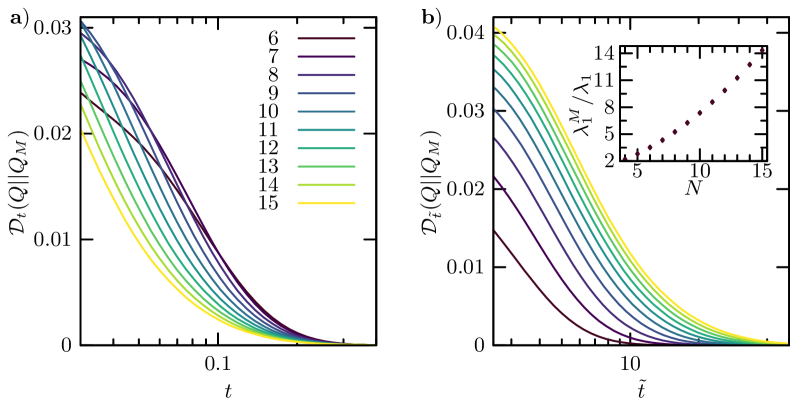
Figure 2: The Kullback-Leibler divergence between the exact non-Markovian Green’s function $Q(q_{3},t|q_{0,3})$ and the Markovian approximation $Q_{M}(q_{3},t|q_{0,3})$ as a function of time (measured in units of collision time) for increasing values of particle numbers $N$: a) results shown on the absolute (dimensionless) time-scale and b) on the natural time-scale, that is, expressed in units of collision time $\tilde{t}$. Inset: $\lambda_{1}^{M}$, the slowest relaxation rate of $Q_{M}(q_{3},t|q_{0,3})$ compared to the corresponding eigenvalue $\lambda_{1}$ of the exact $Q(q_{3},t|q_{0,3})$.

The results $\mathcal{D}_{t}(Q||Q_{M})$ are shown in Fig. 2. From Fig. 2 we confirm that the Markovianity is broken transiently (on time-scales $t\lesssim\lambda_{\mathbf{1}}^{-1}$, which holds for any ergodic dynamics in the sense of generating an invariant measure. Notably, the relaxation time $\lambda_{\mathbf{1}}$ does not depend on $N$ and is hence equal for all cases considered here. Moreover, as expected, the magnitude of broken Markovianity increases with the ’degree’ of the projection (here with the particle number $N$), as is best seen on a natural time-scale (see Fig. 2b). Conversely, on the absolute time-scale the relaxation rate of the Markovian approximation, describing diffusion on a free energy landscape $f(q_{3})=-\beta\ln\Psi_{\mathbf{00}}(q_{3})$, which can be defined as

$$\lambda^{M}_{1}=-\lim_{t\to\infty}t^{-1}\ln(Q_{M}(q_{j},t|q_{0,j})-\Psi_{\mathbf{00}}(q_{j}))$$ (37)

increases with increasing $N$ (see inset in Fig. 2b). Therefore, while both have by construction the same invariant measure, the Markovian approximation overestimates the rate of relaxation. This highlights the pitfall in using free energy landscape ideas in absence of a time-scale separation.

4.4 Tagged Particle Local Times Probing the Origin of Broken Markovianity

In order to gain deeper insight into the origin and physical meaning of memory emerging from integrating out latent degrees of freedom we inspect how a given tagged particle explores the configuration space starting from a stationary (equilibrium) initial condition. To that end we first compute the variance of local time of a tagged particle, $\theta_{t}(q_{j})$ in Eq. (24), given in the general form in Eq. (25), which applied to tagged particle diffusion in a tilted single file reads:

$$\sigma^{2}_{t}(q_{j})=2\sum_{\mathbf{k}}\frac{\Psi_{\mathbf{0k}}(q_{j})\Psi_{\mathbf{k0}}(q_{j})}{\lambda_{\mathbf{k}}t}\left(1-\frac{1-\mathrm{e}^{-\lambda_{\mathbf{k}}t}}{\lambda_{\mathbf{k}}t}\right)$$ (38)

where $\Psi_{\mathbf{k0}}(q_{j})$ is given by Eq. (33) and $\Psi_{\mathbf{0k}}(q_{j})=\frac{\mathbf{m}_{\mathbf{k}}!}{N!}\Psi_{\mathbf{k0}}(q_{j})$. Note that since the process in ergodic we have $\langle\theta_{t}(q_{j})\rangle=\Psi_{\mathbf{00}}(q_{j})$, and because the projected dynamics becomes asymptotically Gaussian (i.e. the correlations between $\theta_{t}(q_{j})$ at different $t$ gradually decorrelate) we also have the large deviation $\lim_{t\to\infty}t\sigma^{2}_{t}(q_{j})=2\sum_{\mathbf{k}}\lambda_{\mathbf{k}}^{-1}\Psi_{\mathbf{0k}}(q_{j})\Psi_{\mathbf{k0}}(q_{j})\neq f(t)$. Moreover, because of detailed balance the large deviation principle represents an upper bound to fluctuations of time-average observables $\sigma^{2}_{t}(q_{j})\leq 2\sum_{\mathbf{k}}\frac{\Psi_{\mathbf{0k}}(q_{j})\Psi_{\mathbf{k0}}(q_{j})}{\lambda_{\mathbf{k}}t},\forall t$.

In order to gain more intuition we inspect the statistics of $\theta_{t}(q_{j})$ for a single file of four particles (see Fig. 3) at different lengths of trajectory $t$ (plotted here on the absolute time-scale). In Fig. 3 we show $\langle\theta_{t}(q_{j})\rangle$ with full lines, and the region bounded by the standard deviation $\pm\sigma_{t}(q_{j})$ with the shaded area.

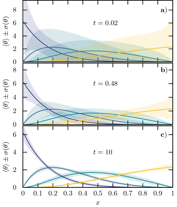
Figure 3: Statistics of tagged particle local time for all members of a single file of four particles starting from stationary initial conditions; $\langle\theta_{t}(q_{j})\rangle$ is represented by full lines and the region bounded by the standard deviation $\pm\sigma_{t}(q_{j})$ with the corresponding shaded area. The color code is: $j=1$ violet, $j=2$ blue, $j=3$, green and $j=4$ yellow. The relaxation time corresponds to $\lambda_{\mathbf{1}}^{-1}\simeq 0.1$. Therefore, panel a) depicts fluctuations on a time scale much shorter that $\lambda_{\mathbf{1}}^{-1}$, whereas b) and c) already belong deeply into the ergodic large deviation regime.

The scatter of $\theta_{t}(q_{j})$ is largest near the respective free energy minima.

To understand further how this coupling to non-relaxed latent degrees of freedom arises we inspect the correlations between tagged particle histories

$$\mathcal{C}_{t}(q_{i};q_{j})=\sum_{\mathbf{k}}\frac{\Psi_{\mathbf{0k}}(q_{i})\Psi_{\mathbf{k0}}(q_{j})+\Psi_{\mathbf{0k}}(q_{j})\Psi_{\mathbf{k0}}(q_{i})}{\lambda_{k}t}\left(1-\frac{1-\mathrm{e}^{-\lambda_{k}t}}{\lambda_{k}t}\right),$$ (39)

where as before $\lim_{t\to\infty}t\mathcal{C}_{t}(q_{i};q_{j})\equiv\overline{\mathcal{C}}_{t}(q_{i};q_{j})=\sum_{\mathbf{k}}\lambda_{\mathbf{k}}^{-1}(\Psi_{\mathbf{0k}}(q_{i})\Psi_{\mathbf{k0}}(q_{j})+\Psi_{\mathbf{0k}}(q_{j})\Psi_{\mathbf{k0}}(q_{i}))\neq f(t)$ as a manifestation of the central limit theorem, since $\theta_{t}(q_{i})$ and $\theta_{t}(q_{j})$ asymptotically decorrelate. In other words, taking $\mathcal{C}_{t}(q_{i};q_{i})\equiv\sigma^{2}_{t}(q_{i})$, the complete large deviation statistics of $\theta_{t}(q_{i})$ (i.e. on ergodically long time-scales) is a $N$-dimensional Gaussian with covariance matrix $t^{-1}\overline{\mathcal{C}}_{t}(q_{i};q_{j})$.

To visualize these results we present in Figs. 4 and 5 two-tag nearest neighbor and next-nearest correlations, $\mathcal{C}_{t}(q_{1};q_{3})$ and as $\mathcal{C}_{t}(q_{2};q_{3})$ respectively, for a single file of $N=4$ and $N=7$ particles at two different trajectory lengths.

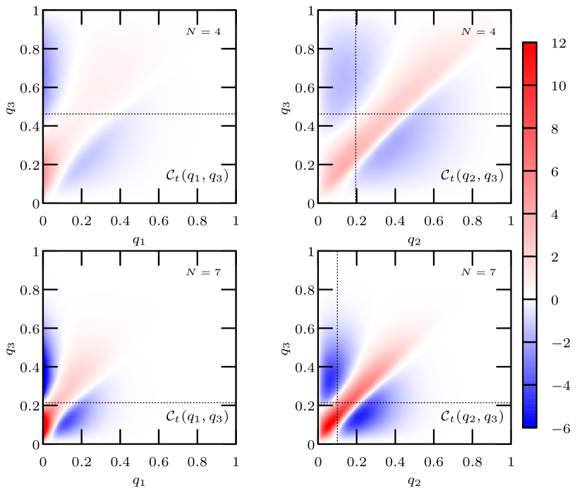
Figure 4: Two-tag local time correlations $\mathcal{C}_{t}(q_{1};q_{3})$ (left) and $\mathcal{C}_{t}(q_{2};q_{3})$ (right) for a single file of $N=4$ (top) and $N=7$ (bottom) particles for a (very short) trajectory length $t=0.01$. The relaxation time corresponds to $\lambda_{\mathbf{1}}^{-1}\simeq 0.1$. The dashed lines denote the positions of the two free energy minima.

We find that, alongside the fact that correlations intuitively increase with the $N$, both the magnitude and the sign of $\mathcal{C}_{t}$ depend on which particles we tag and even more so, where we tag these particles. Along the (upward shifted) diagonal $\mathcal{C}_{t}$ is positive, implying the two tagged particles along a stochastic many-body trajectory effectively (in the sense of the local time) move together, such that if one particle spends more time in a given region, so will the other. At fixed $F$ (here assumed to be equal to 1) the magnitude of the upward shift depends on which particles we tag as well as on $N$. This intuitive idea is backed up mathematically by realizing that the lowest excited Bethe-eigenfunctions correspond to collective (’in phase’) motion (see Eqs. (28) and (29)). Furthermore, defining the free energy minima of the tagged particles with $q^{\text{min}}_{i}$ and $q^{\text{min}}_{i}$ (see dashed lines in Figs. 4 and 5) we would expect, if the particles were to explore their respective free energy minima, a peak localized at $(q^{\text{min}}_{i},q^{\text{min}}_{i})$ (i.e. at the crossing of dashed line in Figs. 4 and 5) . We find, however, that this is not the case, all together implying that the tagged particles do not, along a many-body trajectory, explore their respective free energy minima. Instead, as mentioned above, they move collectively close to each other. The collective dynamics is therefore non-trivial and the tagged particle dynamics cannot be, at least for $t\lesssim\lambda_{1}^{-1}$ coarse grained to a Markovian diffusion on $-\beta\ln\Psi_{\mathbf{00}}(q_{j})$, the free energy landscape of the tagged particle $j$. Conversely, the fact that all correlations (positive and negative) die our as $q_{i,j}\to 1$ is a straightforward consequence of the tilting of the confining box.

Focusing now on the dependence on the length of the trajectory we see at very short time (much shorter than the relaxation time) the correlations are stronger, and that positive correlations peak further away from the two respective tagged particle free energy minima (compare Figs. 4 and 5). In addition, the maximum of $\mathcal{C}_{t}(q_{i};q_{j})$ appears to be somewhat more localized at longer (nearly ergodic) times (see 5). In addition, the tagged particle dynamics seem to be localized more strongly near the free energy minimum if we tag the first particle and if $N$ is larger, presumably because of a faster relaxation due to the presence of the wall effecting more frequent collisions with the wall, during which the particle eventually loses memory.

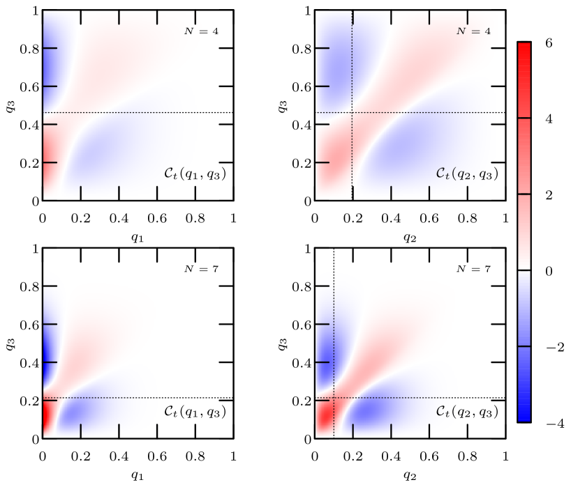
Figure 5: Two-tag local time correlations $\mathcal{C}_{t}(q_{1};q_{3})$ (left) and $\mathcal{C}_{t}(q_{2};q_{3})$ (right) for a single file of $N=4$ (top) and $N=7$ (bottom) particles for a trajectory length comparable to the relaxation time $t=0.12\simeq\lambda_{\mathbf{1}}^{-1}$. The relaxation time corresponds to $\lambda_{\mathbf{1}}^{-1}\simeq 0.1$. The dashed lines denote the positions of the two free energy minima.

5 Summary and Outlook

Non-Markovian dynamics and anomalous diffusion are particularly ubiquitous and important in biophysical systems [1, 2, 3, 4, 5, 6, 7, 8, 9, 10, 11, 12, 13, 14, 15, 16]. There, however, it appears that the quite many non-Markovian observations are described theoretically by phenomenological approaches with ad hoc memory kernels, which in specific cases can lead to mathematically unsound or even unphysical behavior [80]. It therefore seems timely and useful to provide a theoretical perspective of non-Markovian dynamics starting from more fine-grained principles and considering a projection to some effective lower-dimensional configuration space.

The ideas presented here are neither new nor completely general. Projection-operator concepts date back to the original works by Zwanzig, Mori, Nakajima, van Kampen, Hänggi and other pioneers. However, these seminal contributions focused mostly on the analysis of non-Markovian evolution equations, whereas here we provide a thorough analysis of the manifestations of the projection on the level of Green’s functions with the aim to somewhat relieve the need for choosing a particular model based solely on physical intuition. Furthermore, we rigorously establish conditions under which the projected dynamics become Markovian and renewal-type, and derive Markovian approximations to projected generators. As a diagnostic tool we propose a novel framework for the assessment of the degree of broken Markovianity as well as for the elucidation of the origins of non-Markovian behavior.

An important remark concerns the transience of broken Markovianity, which is a consequence of the fact that we assumed that the complete dynamics is ergodic. First we note that (i) for any finite observation of length $t$ it is de facto not possible to discern whether the observation (and the dynamics in general) will be ergodic or not on a time scale $\tau>t$. (ii) All physical observations are (trivially) finite. (iii) In a nominally ergodic dynamics on any finite time scale $t$, where the dynamics starting from some non-stationary initial condition $\mathbf{x}_{0}$ has not yet reached the steady state (in the language of this work $t<\lambda_{1}^{-1}$), it is not possible to observe the effect of a sufficiently distant confining boundary $\partial\Omega(\mathbf{x})$ (potentially located at infinity if the drift field $\mathbf{F}(\mathbf{x})$ is sufficiently confining) that would assure ergodicity (in the language of this work $\forall t\ll\lambda_{1}^{-1}$ such that $G(\bm{l}_{\mathrm{min}},t|\mathbf{x}_{0},0)\simeq 0$ where $|\bm{l}_{\mathrm{min}}|\equiv\mathrm{min}_{\mathbf{x}}|\mathbf{x}_{0}-\partial\Omega(\mathbf{x})|$). Therefore no generality is lost in our work by assuming that the complete dynamics is nominally ergodic, even in a rigorous treatment of so-called weakly non-ergodic dynamics with diverging mean waiting times (see e.g. [1, 6]) or generalized Langevin dynamics with diverging correlation times (see e.g. [29, 30, 31, 32, 33, 34]) on finite time-scales. As a corollary, in the description of such dynamics on any finite time-scale it is a priori by no means necessary to assume that the dynamics is non-ergodic or has a diverging correlation time. This does not imply, however, that the assumption of diverging mean waiting times or diverging correlation times cannot render the analysis of specific models simpler.

Notably, our work considers parent dynamics with a potentially broken time-reversal symmetry and hence includes the description of projection-induced non-Markovian dynamics in non-equilibrium (i.e. irreversible) systems. In the latter case the relaxation process of the parent microscopic process might not be monotonic (i.e. may oscillate), and it will be very interesting to explore the manifestations and importance of these oscillations in projected non-Markovian dynamics.

In the context of renewal dynamics our work builds on firm mathematical foundations of Markov processes and therefore provides mathematically and physically consistent explicit (but notably not necessarily the most general) memory kernels derived from microscopic (or fine-grained) principles, which can serve for the development, assessment and fine-tuning of empirical memory kernels that are used frequently in the theoretical modeling of non-Markovian phenomena (e.g. power-law, exponential, stretched exponential etc; [2, 80]). In particular, power-law kernels are expected to emerge as transients in cases, where the latent degrees of freedom relax over multiple time-scales with a nearly continuous and self-similar spectrum. Conversely, the quite strongly restrictive conditions imposed on the microscopic (parent) dynamics that lead to renewal dynamics, which we reveal here, suggest that renewal type transport in continuous space (e.g. continuous-time random walks [1, 2]) might not be the most abundant processes underlying projection-induced non-Markovian dynamics in physical systems, but are more likely to arise due to some disorder averaging. In general, it seems natural that coarse graining involving some degree of spatial discretization should underly renewal type ideas.

From a more general perspective beyond the theory of anomalous diffusion our results are relevant for the description and understanding of experimental observables $a(\mathbf{q})$ coupled to projected dynamics $\mathbf{q}(t)$ in presence of slow latent degrees of freedom (e.g. a FRET experiment measuring the distance within a protein or a DNA molecule [86]), as well as for exploring stochastic thermodynamic properties of projected dynamics with slow hidden degrees of freedom [87, 88, 89]. An important field of applications of the spectral-theoretic ideas developed here is the field of statistical kinetics in the context of first passage concepts (e.g. [90, 91, 92]), where general results for non-Markovian dynamics are quite sparse [93, 94, 95, 49, 96, 97, 98, 99] and will be the subject of our future studies.

Conflict of Interest Statement

The authors declare that the research was conducted in the absence of any commercial or financial relationships that could be construed as a potential conflict of interest.

Author Contributions

AL and AG conceived the research, performed the research, and wrote and reviewed the paper.

Funding

The financial support from the German Research Foundation (DFG) through the Emmy Noether Program ‘GO 2762/1-1’ (to AG), and an IMPRS fellowship of the Max Planck Society (to AL) are gratefully acknowledged.

References

- Metzler and Klafter [2000a] Metzler R, Klafter J. The random walk’s guide to anomalous diffusion: a fractional dynamics approach. Physics Reports 339 (2000a) 1 – 77. https://doi.org/10.1016/S0370-1573(00)00070-3.
- Metzler and Klafter [2004] Metzler R, Klafter J. The restaurant at the end of the random walk: recent developments in the description of anomalous transport by fractional dynamics. J. Phys. A.: Math. Gen. 37 (2004) R161–R208. https://doi.org/10.1088/0305-4470/37/31/R01.
- Sokolov and Klafter [2005] Sokolov IM, Klafter J. From diffusion to anomalous diffusion: A century after Einstein’s Brownian motion. Chaos 15 (2005) 026103. https://doi.org/10.1063/1.1860472.
- Klages et al. [2008] Klages R, Radons G, Sokolov IM. Anomalous Transport: Foundations and Applications (Weinheim: Wiley‐VCH Verlag GmbH and Co.) (2008).
- Godec et al. [2014a] Godec A, Bauer M, Metzler R. Collective dynamics effect transient subdiffusion of inert tracers in flexible gel networks. New Journal of Physics 16 (2014a) 092002. 10.1088/1367-2630/16/9/092002.
- Metzler et al. [2014] Metzler R, Jepn JH, Cherstvy AG, Barkai E. Anomalous diffusion models and their properties: non-stationarity, non-ergodicity, and ageing at the centenary of single particle tracking. Phys. Chem. Chem. Phys. 16 (2014) 24128–24164. 10.1039/C4CP03465A.
- Höfling and Franosch [2013] Höfling F, Franosch T. Anomalous transport in the crowded world of biological cells. Reports on Progress in Physics 76 (2013) 046602. 10.1088/0034-4885/76/4/046602.
- Sokolov [2012] Sokolov IM. Models of anomalous diffusion in crowded environments. Soft Matter 8 (2012) 9043–9052. 10.1039/C2SM25701G.
- Metzler et al. [2016] Metzler R, Jeon JH, Cherstvy AG. Non-Brownian diffusion in lipid membranes: Experiments and simulations. Biochimica et Biophysica Acta (BBA) - Biomembranes 1858 (2016) 2451 – 2467. https://doi.org/10.1016/j.bbamem.2016.01.022. Biosimulations of lipid membranes coupled to experiments.
- Oliveira et al. [2019] Oliveira FA, Ferreira RMS, Lapas LC, Vainstein MH. Anomalous diffusion: A basic mechanism for the evolution of inhomogeneous systems. Frontiers in Physics 7 (2019) 18. 10.3389/fphy.2019.00018.
- Woringer and Darzacq [2018] Woringer M, Darzacq X. Protein motion in the nucleus: from anomalous diffusion to weak interactions. Biochemical Society Transactions (2018). 10.1042/BST20170310.
- Dix and Verkman [2008] Dix JA, Verkman AS. Crowding effects on diffusion in solutions and cells. Annual Review of Biophysics 37 (2008) 247–263. 10.1146/annurev.biophys.37.032807.125824. PMID: 18573081.
- Krapf [2015] Krapf D. Chapter five - mechanisms underlying anomalous diffusion in the plasma membrane. Kenworthy AK, editor, Lipid Domains (Academic Press), Current Topics in Membranes, vol. 75 (2015), 167 – 207. https://doi.org/10.1016/bs.ctm.2015.03.002.
- Golding and Cox [2006] Golding I, Cox EC. Physical nature of bacterial cytoplasm. Phys. Rev. Lett. 96 (2006) 098102. 10.1103/PhysRevLett.96.098102.
- Jeon et al. [2016] Jeon JH, Javanainen M, Martinez-Seara H, Metzler R, Vattulainen I. Protein crowding in lipid bilayers gives rise to non-gaussian anomalous lateral diffusion of phospholipids and proteins. Phys. Rev. X 6 (2016) 021006. 10.1103/PhysRevX.6.021006.
- Rienzo et al. [2014] Rienzo CD, Piazza V, Gratton E, Beltram F, Cardarelli F. Probing short-range protein Brownian motion in the cytoplasm of living cells. Nature Comminications 5 (2014) 5891. 10.1038/ncomms6891.
- Metzler and Klafter [2007] Metzler R, Klafter J. Anomalous Stochastic Processes in the Fractional Dynamics Framework: Fokker-Planck Equation, Dispersive Transport, and Non-Exponential Relaxation (John Wiley and Sons, Ltd) (2007), 223 . 10.1002/9780470141762.ch3.
- Lomholt et al. [2013] Lomholt MA, Lizana L, Metzler R, Ambjörnsson T. Microscopic origin of the logarithmic time evolution of aging processes in complex systems. Phys. Rev. Lett. 110 (2013) 208301. 10.1103/PhysRevLett.110.208301.
- Bouchaud and Georges [1990] Bouchaud JP, Georges A. Anomalous diffusion in disordered media: Statistical mechanisms, models and physical applications. Physics Reports 195 (1990) 127 – 293. https://doi.org/10.1016/0370-1573(90)90099-N.
- Bouchaud et al. [1990] Bouchaud J, Comtet A, Georges A, Doussal PL. Classical diffusion of a particle in a one-dimensional random force field. Annals of Physics 201 (1990) 285 – 341. https://doi.org/10.1016/0003-4916(90)90043-N.
- Sinai [1982] Sinai YG. The limiting behavior of a one-dimensional random walk in a random medium. Theory Prob. Appl. 27 (1982) 285 – 341. https://doi.org/10.1137/1127028.
- Oshanin et al. [2013] Oshanin G, Rosso A, Schehr G. Anomalous fluctuations of currents in sinai-type random chains with strongly correlated disorder. Phys. Rev. Lett. 110 (2013) 100602. 10.1103/PhysRevLett.110.100602.
- Dean et al. [2014] Dean DS, Gupta S, Oshanin G, Rosso A, Schehr G. Diffusion in periodic, correlated random forcing landscapes. Journal of Physics A: Mathematical and Theoretical 47 (2014) 372001. 10.1088/1751-8113/47/37/372001.
- Radons [2004] Radons G. Anomalous transport in disordered dynamical systems. Physica D: Nonlinear Phenomena 187 (2004) 3 – 19. https://doi.org/10.1016/j.physd.2003.09.001. Microscopic Chaos and Transport in Many-Particle Systems.
- Godec et al. [2014b] Godec A, Chechkin AV, Barkai E, Kantz H, Metzler R. Localisation and universal fluctuations in ultraslow diffusion processes. Journal of Physics A: Mathematical and Theoretical 47 (2014b) 492002. 10.1088/1751-8113/47/49/492002.
- Krüsemann et al. [2014] Krüsemann H, Godec A, Metzler R. First-passage statistics for aging diffusion in systems with annealed and quenched disorder. Phys. Rev. E 89 (2014) 040101. 10.1103/PhysRevE.89.040101.
- Krüsemann et al. [2015] Krüsemann H, Godec A, Metzler R. Ageing first passage time density in continuous time random walks and quenched energy landscapes. Journal of Physics A: Mathematical and Theoretical 48 (2015) 285001. 10.1088/1751-8113/48/28/285001.
- Coffey et al. [1996] Coffey WT, Kalmykov YP, Waldron JT. The Langevin Equation (WORLD SCIENTIFIC) (1996). 10.1142/2256.
- Jeon and Metzler [2010] Jeon JH, Metzler R. Fractional Brownian motion and motion governed by the fractional Langevin equation in confined geometries. Phys. Rev. E 81 (2010) 021103. 10.1103/PhysRevE.81.021103.
- Lutz [2001] Lutz E. Fractional Langevin equation. Phys. Rev. E 64 (2001) 051106. 10.1103/PhysRevE.64.051106.
- Deng and Barkai [2009] Deng W, Barkai E. Ergodic properties of fractional Brownian-Langevin motion. Phys. Rev. E 79 (2009) 011112. 10.1103/PhysRevE.79.011112.
- Metzler and Klafter [2000b] Metzler R, Klafter J. Subdiffusive transport close to thermal equilibrium: From the Langevin equation to fractional diffusion. Phys. Rev. E 61 (2000b) 6308–6311. 10.1103/PhysRevE.61.6308.
- Kou and Xie [2004] Kou SC, Xie XS. Generalized Langevin equation with fractional gaussian noise: Subdiffusion within a single protein molecule. Phys. Rev. Lett. 93 (2004) 180603. 10.1103/PhysRevLett.93.180603.
- Burov and Barkai [2008] Burov S, Barkai E. Critical exponent of the fractional Langevin equation. Phys. Rev. Lett. 100 (2008) 070601. 10.1103/PhysRevLett.100.070601.
- Goychuk [2012] Goychuk I. Viscoelastic Subdiffusion: Generalized Langevin Equation Approach (John Wiley and Sons, Ltd) (2012), 187 . 10.1002/9781118197714.ch5.
- Dubkov et al. [2009] Dubkov AA, Hänggi P, Goychuk I. Non-linear Brownian motion: the problem of obtaining the thermal Langevin equation for a non-gaussian bath. Journal of Statistical Mechanics: Theory and Experiment 2009 (2009) P01034. 10.1088/1742-5468/2009/01/p01034.
- Cherstvy et al. [2013] Cherstvy AG, Chechkin AV, Metzler R. Anomalous diffusion and ergodicity breaking in heterogeneous diffusion processes. New Journal of Physics 15 (2013) 083039. 10.1088/1367-2630/15/8/083039.
- Cherstvy and Metzler [2014] Cherstvy AG, Metzler R. Nonergodicity, fluctuations, and criticality in heterogeneous diffusion processes. Phys. Rev. E 90 (2014) 012134. 10.1103/PhysRevE.90.012134.
- Massignan et al. [2014] Massignan P, Manzo C, Torreno-Pina JA, García-Parajo MF, Lewenstein M, Lapeyre GJ. Nonergodic subdiffusion from Brownian motion in an inhomogeneous medium. Phys. Rev. Lett. 112 (2014) 150603. 10.1103/PhysRevLett.112.150603.
- Guérin and Dean [2015] Guérin T, Dean DS. Force-induced dispersion in heterogeneous media. Phys. Rev. Lett. 115 (2015) 020601. 10.1103/PhysRevLett.115.020601.
- Godec and Metzler [2015a] Godec A, Metzler R. Optimization and universality of Brownian search in a basic model of quenched heterogeneous media. Phys. Rev. E 91 (2015a) 052134. 10.1103/PhysRevE.91.052134.
- Vaccario et al. [2015] Vaccario G, Antoine C, Talbot J. First-passage times in -dimensional heterogeneous media. Phys. Rev. Lett. 115 (2015) 240601. 10.1103/PhysRevLett.115.240601.
- Godec and Metzler [2016] Godec A, Metzler R. First passage time distribution in heterogeneity controlled kinetics: going beyond the mean first passage time. Sci. Rep. 6 (2016) 20349. 10.1038/srep20349.
- Chubynsky and Slater [2014] Chubynsky MV, Slater GW. Diffusing diffusivity: A model for anomalous, yet Brownian, diffusion. Phys. Rev. Lett. 113 (2014) 098302. 10.1103/PhysRevLett.113.098302.
- Chechkin et al. [2017] Chechkin AV, Seno F, Metzler R, Sokolov IM. Brownian yet non-gaussian diffusion: From superstatistics to subordination of diffusing diffusivities. Phys. Rev. X 7 (2017) 021002. 10.1103/PhysRevX.7.021002.
- Godec and Metzler [2017a] Godec A, Metzler R. First passage time statistics for two-channel diffusion. Journal of Physics A: Mathematical and Theoretical 50 (2017a) 084001. 10.1088/1751-8121/aa5204.
- Sposini et al. [2018] Sposini V, Chechkin AV, Seno F, Pagnini G, Metzler R. Random diffusivity from stochastic equations: comparison of two models for Brownian yet non-gaussian diffusion. New Journal of Physics 20 (2018) 043044. 10.1088/1367-2630/aab696.
- Lanoiselée and Grebenkov [2018] Lanoiselée Y, Grebenkov DS. A model of non-gaussian diffusion in heterogeneous media. Journal of Physics A: Mathematical and Theoretical 51 (2018) 145602. 10.1088/1751-8121/aab15f.
- Grebenkov [2019] Grebenkov DS. A unifying approach to first-passage time distributions in diffusing diffusivity and switching diffusion models. Journal of Physics A: Mathematical and Theoretical 52 (2019) 174001. 10.1088/1751-8121/ab0dae.
- Lanoiselee et al. [2018] Lanoiselee Y, Moutal N, Grebenkov DS. Diffusion-limited reactions in dynamic heterogeneous media. Nature Comminications 9 (2018) 4398. 10.1088/1751-8121/ab0dae.
- Zwanzig [1960] Zwanzig R. Ensemble method in the theory of irreversibility. The Journal of Chemical Physics 33 (1960) 1338–1341. 10.1063/1.1731409.
- Nordholm and Zwanzig [1975] Nordholm S, Zwanzig R. A systematic derivation of exact generalized Brownian motion theory. Journal of Statistical Physics 13 (1975) 347–371. 10.1007/BF01012013.
- Mori [1965] Mori H. Transport, Collective Motion, and Brownian Motion*). Progress of Theoretical Physics 33 (1965) 423–455. 10.1143/PTP.33.423.
- Grabert et al. [1977] Grabert H, Talkner P, Hänggi P. Microdynamics and time-evolution of macroscopic non-Markovian systems. Zeitschrift für Physik B Condensed Matter 26 (1977) 389–395. 10.1007/BF01570749.
- Hänggi and Thomas [1977] Hänggi P, Thomas H. Time evolution, correlations, and linear response of non-Markov processes. Zeitschrift für Physik B Condensed Matter 26 (1977) 85–92. 10.1007/BF01313376.
- Grabert et al. [1978] Grabert H, Talkner P, Hänggi P, Thomas H. Microdynamics and time-evolution of macroscopic non-Markovian systems. ii. Zeitschrift für Physik B Condensed Matter 29 (1978) 273–280. 10.1007/BF01321192.
- Hynes et al. [1975] Hynes J, Kapral R, Weinberg M. Microscopic theory of Brownian motion: Mori friction kernel and Langevin-equation derivation. Physica A: Statistical Mechanics and its Applications 80 (1975) 105 – 127. https://doi.org/10.1016/0378-4371(75)90162-4.
- Haken [1975] Haken H. Cooperative phenomena in systems far from thermal equilibrium and in nonphysical systems. Rev. Mod. Phys. 47 (1975) 67–121. 10.1103/RevModPhys.47.67.
- Ferrario and Grigolini [1979] Ferrario M, Grigolini P. The non‐Markovian relaxation process as a “contraction” of a multidimensional one of Markovian type. Journal of Mathematical Physics 20 (1979) 2567–2572. 10.1063/1.524019.
- Grigolini [1988] Grigolini P. A fokker–planck equation for canonical non‐Markovian systems: A local linearization approach. The Journal of Chemical Physics 89 (1988) 4300–4308. 10.1063/1.454812.
- Harris [1965] Harris TE. Diffusion with “collisions” between particles. Journal of Applied Probability 2 (1965) 323–338. 10.2307/3212197.
- Lizana and Ambjörnsson [2008] Lizana L, Ambjörnsson T. Single-file diffusion in a box. Phys. Rev. Lett. 100 (2008) 200601. 10.1103/PhysRevLett.100.200601.
- Barkai and Silbey [2009] Barkai E, Silbey R. Theory of single file diffusion in a force field. Phys. Rev. Lett. 102 (2009) 050602. 10.1103/PhysRevLett.102.050602.
- Sanders et al. [2014] Sanders LP, Lomholt MA, Lizana L, Fogelmark K, Metzler R, Ambjörnsson T. Severe slowing-down and universality of the dynamics in disordered interacting many-body systems: ageing and ultraslow diffusion. New Journal of Physics 16 (2014) 113050. 10.1088/1367-2630/16/11/113050.
- Illien et al. [2013] Illien P, Bénichou O, Mejía-Monasterio C, Oshanin G, Voituriez R. Active transport in dense diffusive single-file systems. Phys. Rev. Lett. 111 (2013) 038102. 10.1103/PhysRevLett.111.038102.
- Bertrand et al. [2018] Bertrand T, Illien P, Bénichou O, Voituriez R. Dynamics of run-and-tumble particles in dense single-file systems. New Journal of Physics 20 (2018) 113045. 10.1088/1367-2630/aaef6f.
- Lapolla and Godec [2018] Lapolla A, Godec A. Unfolding tagged particle histories in single-file diffusion: exact single- and two-tag local times beyond large deviation theory. New Journal of Physics 20 (2018) 113021. 10.1088/1367-2630/aaea1b.
- Godec and Metzler [2015b] Godec A, Metzler R. Signal focusing through active transport. Phys. Rev. E 92 (2015b) 010701. 10.1103/PhysRevE.92.010701.
- Deutch and Silbey [1971] Deutch JM, Silbey R. Exact generalized Langevin equation for a particle in a harmonic lattice. Phys. Rev. A 3 (1971) 2049–2052. 10.1103/PhysRevA.3.2049.
- Havlin et al. [1987] Havlin S, Kiefer JE, Weiss GH. Anomalous diffusion on a random comblike structure. Phys. Rev. A 36 (1987) 1403–1408. 10.1103/PhysRevA.36.1403.
- Pottier [1994] Pottier N. Analytic study of a model of diffusion on random comb-like structures. Il Nuovo Cimento D 16 (1994) 1223–1230. 10.1007/BF02458804.
- Berezhkovskii et al. [2014] Berezhkovskii AM, Dagdug L, Bezrukov SM. From normal to anomalous diffusion in comb-like structures in three dimensions. The Journal of Chemical Physics 141 (2014) 054907. 10.1063/1.4891566.
- Qian [2013] Qian H. A decomposition of irreversible diffusion processes without detailed balance. Journal of Mathematical Physics 54 (2013) 053302. 10.1063/1.4803847.
- Helffer and Nier [2005] Helffer B, Nier F. Hypoelliptic Estimates and Spectral Theory for Fokker-Planck Operators and Witten Laplacians (Heidelberg: Springer, Berlin, Heidelberg) (2005). 10.1007/b104762.
- Chupin [2010] Chupin L. Fokker-Planck equation in bounded domain. Ann. Inst. Fourier. 60 (2010) 217. 10.5802/aif.2521.
- Reed and Simon [1972] Reed M, Simon B. Methods of Modern Mathematical Physics I: Functional Analysis (New York: Academic Press) (1972). 10.1016/B978-0-12-585001-8.X5001-6.
- Conway [1985] Conway JB. A Course in Functional Analysis (New York: Springer-Verlag New York) (1985). 10.1007/978-1-4757-3828-5.
- Feller [1959] Feller W. Non-Markovian processes with the semigroup property. Ann. Math. Statist. 30 (1959) 1252–1253. 10.1214/aoms/1177706110.
- Hanggi et al. [1978] Hanggi P, Thomas H, Grabert H, Talkner P. Note on time evolution of non-Markov processes. Journal of Statistical Physics 18 (1978) 155–159. 10.1007/BF01014306.
- Sokolov [2002] Sokolov IM. Solutions of a class of non-Markovian fokker-planck equations. Phys. Rev. E 66 (2002) 041101. 10.1103/PhysRevE.66.041101.
- Risken and Haken [1989] Risken H, Haken H. The Fokker-Planck Equation: Methods of Solution and Applications Second Edition (Springer) (1989).
- Polettini [2013] Polettini M. Generally covariant state-dependent diffusion. Journal of Statistical Mechanics: Theory and Experiment 2013 (2013) P07005. 10.1088/1742-5468/2013/07/p07005.
- Polettini and Esposito [2013] Polettini M, Esposito M. Nonconvexity of the relative entropy for Markov dynamics: A fisher information approach. Phys. Rev. E 88 (2013) 012112. 10.1103/PhysRevE.88.012112.
- Korepin et al. [1993] Korepin VE, Bogoliubov NM, Izergin AG. Quantum Inverse Scattering Method and Correlation Functions. Cambridge Monographs on Mathematical Physics (Cambridge University Press) (1993). 10.1017/CBO9780511628832.
- Lizana and Ambjörnsson [2009] Lizana L, Ambjörnsson T. Diffusion of finite-sized hard-core interacting particles in a one-dimensional box: Tagged particle dynamics. Phys. Rev. E 80 (2009) 051103. 10.1103/PhysRevE.80.051103.
- Gopich and Szabo [2012] Gopich IV, Szabo A. Theory of the energy transfer efficiency and fluorescence lifetime distribution in single-molecule fret. Proceedings of the National Academy of Sciences 109 (2012) 7747–7752. 10.1073/pnas.1205120109.
- Seifert [2012] Seifert U. Stochastic thermodynamics, fluctuation theorems and molecular machines. Reports on Progress in Physics 75 (2012) 126001. 10.1088/0034-4885/75/12/126001.
- Mehl et al. [2012] Mehl J, Lander B, Bechinger C, Blickle V, Seifert U. Role of hidden slow degrees of freedom in the fluctuation theorem. Phys. Rev. Lett. 108 (2012) 220601. 10.1103/PhysRevLett.108.220601.
- Uhl et al. [2018] Uhl M, Pietzonka P, Seifert U. Fluctuations of apparent entropy production in networks with hidden slow degrees of freedom. Journal of Statistical Mechanics: Theory and Experiment 2018 (2018) 023203. 10.1088/1742-5468/aaa78b.
- Hartich and Godec [2018] Hartich D, Godec A. Duality between relaxation and first passage in reversible Markov dynamics: rugged energy landscapes disentangled. New Journal of Physics 20 (2018) 112002. 10.1088/1367-2630/aaf038.
- Hartich and Godec [2019a] Hartich D, Godec A. Interlacing relaxation and first-passage phenomena in reversible discrete and continuous space Markovian dynamics. Journal of Statistical Mechanics: Theory and Experiment 2019 (2019a) 024002. 10.1088/1742-5468/ab00df.
- Hartich and Godec [2019b] Hartich D, Godec A. Extreme value statistics of ergodic Markov processes from first passage times in the large deviation limit. Journal of Physics A: Mathematical and Theoretical 52 (2019b) 244001. 10.1088/1751-8121/ab1eca.
- Hänggi and Talkner [1981] Hänggi P, Talkner P. Non-Markov processes: The problem of the mean first passage time. Zeitschrift für Physik B Condensed Matter 45 (1981) 79–83. 10.1007/BF01294279.
- Balakrishnan et al. [1988] Balakrishnan V, Van den Broeck C, Hänggi P. First-passage times of non-Markovian processes: The case of a reflecting boundary. Phys. Rev. A 38 (1988) 4213–4222. 10.1103/PhysRevA.38.4213.
- McKane et al. [1990] McKane AJ, Luckock HC, Bray AJ. Path integrals and non-Markov processes. i. general formalism. Phys. Rev. A 41 (1990) 644–656. 10.1103/PhysRevA.41.644.
- Reimann et al. [1999] Reimann P, Schmid GJ, Hänggi P. Universal equivalence of mean first-passage time and kramers rate. Phys. Rev. E 60 (1999) R1–R4. 10.1103/PhysRevE.60.R1.
- Godec and Metzler [2017b] Godec A, Metzler R. First passage time statistics for two-channel diffusion. Journal of Physics A: Mathematical and Theoretical 50 (2017b) 084001. 10.1088/1751-8121/aa5204.
- Bray et al. [2013] Bray AJ, Majumdar SN, Schehr G. Persistence and first-passage properties in nonequilibrium systems. Advances in Physics 62 (2013) 225–361. 10.1080/00018732.2013.803819.
- Guerin et al. [2016] Guerin T, Levernier N, Benichou O, Voituriez R. Mean first-passage times of non-Markovian random walkers in confinement. Nature 534 (2016).