A unified analytical theory of heteropolymers for sequence-specific phase behaviors of polyelectrolytes and polyampholytes

Abstract

The physical chemistry of liquid-liquid phase separation (LLPS) of polymer solutions bears directly on the assembly of biologically functional droplet-like bodies from proteins and nucleic acids. These biomolecular condensates include certain extracellular materials, and intracellular compartments that are characterized as “membraneless organelles”. Analytical theories are a valuable, computationally efficient tool for addressing general principles. LLPS of neutral homopolymers are quite well described by theory; but it has been a challenge to develop general theories for the LLPS of heteropolymers involving charge-charge interactions. Here we present a theory that combines a random-phase-approximation treatment of polymer density fluctuations and an account of intrachain conformational heterogeneity based upon renormalized Kuhn lengths to provide predictions of LLPS properties as a function of pH, salt, and charge patterning along the chain sequence. Advancing beyond more limited analytical approaches, our LLPS theory is applicable to a wide variety of charged sequences ranging from highly charged polyelectrolytes to neutral or nearly neutral polyampholytes. This theory should be useful in high-throughput screening of protein and other sequences for their LLPS propensities and can serve as a basis for more comprehensive theories that incorporate non-electrostatic interactions. Experimental ramifications of our theory are discussed.

I Introduction

Mesoscopic compartmentalization undergirded by liquid-liquid phase separation (LLPS) of intrinsically disordered proteins or regions (IDPs or IDRs) and nucleic acids is now recognized as a versatile means for biomolecular organization and regulation Brangwynne et al. (2009); Li et al. (2012); Kato et al. (2012); Nott et al. (2015); Molliex et al. (2015); Pak et al. (2016). Some of these phase-separated droplet-like compartments are intracellular bodies—such as stress granules, P-granules and nucleoli—that may be characterized as “membraneless organelles”. Outside the cell, biomolecular LLPS can be biologically useful as well, as in the formation of certain extracellular materials. Collectively referred to as biomolecular condensates, these phase-separated bodies participate in many vital functions, as highlighted by their recently elucidated roles in endocytosis Bergeron-Sandoval et al. (2018), silencing chromatin Larson et al. (2017), transcription Plys and Kingston (2018); Cho et al. (2018); Sabari et al. (2018), and translation Tsang et al. (2019). The repertoire of relevant discoveries is rapidly expanding Shin and Brangwynne (2017); Banani et al. (2017); Boeynaems et al. (2018). LLPS of globular proteins, for example lens protein solutions, have also been observed and are of biological importance Broide et al. (1991); Asherie, Lomakin, and Benedek (1996); San Biagio et al. (1999); Zhou and Pang (2018); Qin and Zhou (2016); Cinar et al. (2019a).

Recent bioinformatics analyses suggest that IDPs and IDRs comprise a significant fraction of the proteomes of higher organisms, and that functional LLPS is likely ubiquitous Forman-Kay, Kriwacki, and Seydoux (2018). The propensity for an IDP or IDR to phase separate is governed by its amino acid sequence and modulated by solution/environmental conditions (temperature, hydrostatic pressure Cinar et al. (2019b), pH, ionic strength Brady et al. (2017); Alberti (2017), etc) as well as their interactions with other biopolymers such as RNA. Thus, any “big-picture” survey of the physical basis of biomolecular condensates requires not only consideration of many different sequences but a large variety of environmental conditions. Adding to this combinatorial complexity is that even for a given wildtype sequence, postranslational modifications, mutations, and splicing Nott et al. (2015); Monahan et al. (2017) can lead to diverse LLPS propensities. In this context, analytical theories are the most computationally efficient tool for large-scale exploration of sequence-dependent biomolecular LLPS. Although explicit-chain simulations provide more energetic and structural details Dignon et al. (2018a); Das et al. (2018a); Dignon et al. (2018b) and field-theory simulations afford more numerical accuracy McCarty et al. (2019); Danielsen et al. (2019a, b), currently the number of sequences that can be simulated by these approaches is limited because of their high computational cost. Moreover, analytical theories are valuable for insights into physical principles that are less manifest in simulation studies. With this in mind, we build on recent success in using analytical theories to account for sequence-dependent biomolecular condensates under certain limited conditions Brangwynne, Tompa, and Pappu (2015); Lin, Forman-Kay, and Chan (2018) so as to develop improved theories that are more generally applicable.

Building sequence-specific theories of LLPS will also have implications in phase separation of block polyamphoytes and its comparison with complex coacervation between oppositely charged homopolyelectrolytes, a topic of intense research in polymer physics deJong and Kruyt (1929); Overbeek and Voorn (1957); Spruijt et al. (2010); Chollakup et al. (2010); Perry et al. (2014); Perry and Sing (2015); Srivastava and Tirrell (2016); Lytle, Radhakrishna, and Sing (2016); Lytle and Sing (2017); Radhakrishna et al. (2017); Dubin and Stewart (2018); Zhang et al. (2018); Adhikari, Leaf, and Muthukumar (2018); Li et al. (2018); Madinya et al. (2019). Diblock polyampholytes with repeat units of a polycation segment followed by a polyanion segment can be envisioned to be equivalent to two oppositely charged homopolyelectrolytes. For this reason LLPS of block polyampholytes – a limiting case of our theory – is often termed self-coacervation Danielsen et al. (2019b, a) and shares features similar to complex cocervation of a polycation and polyanion Madinya et al. (2019). Experiments and simulation have also reported differences between the phase diagrams of block polyampholytes and homopolyelectrolyte coacervation. The observed differences can be explained by the presence of ‘charge pattern interfaces’ where two segments of oppositely charged blocks merge in polyampholytes. Homopolyelectrolytes, on the other hand, lack such connectivities, thus leading to different types of salt localization in comparison to block polyampholytes Madinya et al. (2019). Application of a general sequence-based analytical theory of polyampholyte LLPS will further advance these comparisons between complex coacervation and self-coacervation. Future effort in theory development is needed in this direction. Thus, our framework should be useful not only for high-throughput analyses of the LLPS propensities of naturally occurring biological sequences but also for the design of artificial biological and non-biological heteropolymers with desired LLPS properties Chang et al. (2017); Dzuricky, Roberts, and Chilkoti (2018); Lytle et al. (2019).

Inasmuch as sequence-specific analytical theories for biomolecular condensates are concerned, a recent multiple-chain formulation based on the traditional random phase approximation (RPA) Mahdi and Olvera de la Cruz (2000); Ermoshkin and Olvera de la Cruz (2003) has been applied to study the dependence of LLPS of IDPs on the charge patterns along their chain sequences Lin, Forman-Kay, and Chan (2016). This approach accounts for the experimental difference in LLPS propensity between the Ddx4 helicase IDR and its charge-scrambled mutant Lin, Forman-Kay, and Chan (2016); Lin et al. (2017a). It also provides insight into a possible anti-correlation between multiple-chain LLPS propensity and single-chain conformational dimensions Lin and Chan (2017) as well as the degree of demixing of different charge sequences under LLPS conditions Lin et al. (2017b). As an initial step, these advances are useful. As a heteropolymer theory, however, traditional RPA Mahdi and Olvera de la Cruz (2000); Ermoshkin and Olvera de la Cruz (2003) is known to have two main shortcomings. First, the density of monomers of the polymer chains in solution is assumed to be roughly homogeneous as density fluctuations are neglected beyond second order in RPA. A rigorous treatment proposed by Edwards and Muthukumar has shown the importance of including density fluctuations to higher orders Muthukumar (1996, 2018, 2017). Nonetheless, a recent comparison of field-theory simulation and RPA indicates that RPA is reasonably accurate for intermediate to high monomer densities for the cases considered, and that significant deviations between RPA and field theory simulation occur only for volume fraction $<0.02$ that of the highest condensed-phase simulated McCarty et al. (2019). Second, traditional RPA neglects the fact that monomer-monomer interactions can cause conformational variation of individual chains by computing the single-chain structure factor using a Gaussian chain with no intrachain interaction. This limitation, which applies to homopolymers as well as heteropolymers, is particularly acute for the latter. Indeed, experimental and computational studies have shown that single-chain conformational heterogeneities and dimensions are sensitive to sequence specific interactions Hofmann et al. (2012); Das and Pappu (2013); Schuler et al. (2016); Konig et al. (2015); Soranno et al. (2014); Sizemore et al. (2015). Regarding this shortcoming, recently an improved analytical approach was developed at the single-chain level by replacing the Kuhn length $l$ (termed “bare” Kuhn length) of the Gaussian chain by a set of renormalized Kuhn lengths, $l_{1}$, that embodies the sequence-specific interactions approximately Sawle and Ghosh (2015); Firman and Ghosh (2018); Huihui, Firman, and Ghosh (2018). Renormalized structure factors have also been exploited to improve homopolymer LLPS theories for polyelectrolytes Shen and Wang (2017, 2018).

Noting that the first shortcoming described above is likely limited only to regimes of extremely low polymer concentrations, here we first focus on rectifying the second shortcoming by combining the earlier, traditional sequence-dependent RPA theory Lin, Forman-Kay, and Chan (2016); Lin et al. (2017a) with the sequence-dependent single-chain theory that utilizes a renormalized Gaussian (rG) chain formulation Sawle and Ghosh (2015); Firman and Ghosh (2018); Huihui, Firman, and Ghosh (2018) for a better account of conformational heterogeneity. We refer to this theory as rG-RPA. As a control, we also study a simpler theory, analogous to our earlier formulation Lin, Forman-Kay, and Chan (2016); Lin et al. (2017a), that invokes a Gaussian chain with fixed Kuhn length. Following Shen and Wang Shen and Wang (2018), we refer to this $l_{1}=l$ theory as fG-RPA. Extensive comparisons of rG-RPA and fG-RPA predictions on various systems indicate that rG-RPA represents a significant improvement over fG-RPA. As will be detailed below, the superiority of rG-RPA is most notable in its ability to account for the LLPSs of both polyampholytes and polyelectrolytes whereas fG-RPA is inadequate for polyelectrolytic polymers.

II Theory

We consider an overall neutral solution of ${n_{p}}$ charged polymers, each consisting of $N$ monomers (residues), and small ions including ${n_{s}}$ salt ions and ${n_{c}}$ counterions with charge numbers $z_{s}$ and $z_{c}$ respectively. The charge pattern of a polymer is given by an $N$-dimensional vector $|\sigma\rangle=[\sigma_{1},\sigma_{2},...,\sigma_{N}]^{\rm T}$, where $\sigma_{\tau}$ is the charge on the $\tau$th monomer; and $q_{c}\equiv(\sum_{\tau}\sigma_{\tau})/N$ is the net charge per monomer. For simplicity, we consider the case with only one species of positive and one species of negative ions; their numbers are denoted as ${n_{+}}$ and ${n_{-}}$ respectively. Moreover, “salt” is identified as the small ions that carry charges of the same sign as the polymers, whereas “counterions” are the small ions carrying charges opposite to that of the polymers. Thus, ${n_{s}}={n_{+}}$ if $q_{c}>0$ and ${n_{s}}={n_{-}}$ if $q_{c}<0$; and $|q_{c}|{n_{p}}N+z_{s}{n_{s}}=z_{c}{n_{c}}$ for solution neutrality. The densities ($\rho$) of monomers, salt ions, and counterions are, respectively, $\rho_{m}={n_{p}}N/\Omega$, $\rho_{s}={n_{s}}/\Omega$, and $\rho_{c}={n_{c}}/\Omega$, where $\Omega$ is solution volume. Although only a simple system with at most two species of small ions is analyzed here for conceptual clarity, our theory can be readily expanded to account for multiple species of small ions.

Details of our formulation are given in the Appendix. Here we provide the key steps in the derivation. Let $F$ be the total free energy of the system. Then $f\equiv Fl^{3}/(k_{\rm B}T\Omega)$ is free energy in units of $k_{\rm B}T$ per volume $l^{3}$, where $l$ is the bare Kuhn length, $k_{\rm B}$ is Boltzmann constant and $T$ is absolute temperature. In our theory,

$$f=-s+f_{\rm ion}+f_{\rm p}+f_{\rm 0}\;,$$ (1)

where $s$ is mixing entropy, $f_{\rm ion}$ and $f_{\rm p}$ are interactions among the small ions and involving the polymers, respectively, that arise from density fluctuations and $f_{\rm 0}$ is the mean-field excluded volume interaction, all expressed in the same units as $f$. The mixing entropy, which accounts for the configurational freedom of the solutes, takes the Flory-Huggins form, viz.,

$$-s=\frac{\phi_{m}}{N}\ln\phi_{m}+\phi_{s}\ln\phi_{s}+\phi_{c}\ln\phi_{c}+\phi_{w}\ln\phi_{w}\;,$$ (2)

where $\phi_{m}$, $\phi_{s}$, $\phi_{c}$, and $\phi_{w}=1\!-\!\phi_{m}\!-\!\phi_{s}\!-\!\phi_{c}$ are volume fractions ($\phi=\rho l^{3}$), respectively, of polymers, salt ions, counterions, and solvent (water for IDP systems). Following Muthukumar, the charge of each small ion is taken to be distributed over a finite volume comparable to that of a monomer. The corresponding interaction free energy among the small ions is Muthukumar (2002)

$$f_{\rm ion}=-\frac{1}{4\pi}\left[\ln(1+\kappa l)-\kappa l+\frac{1}{2}(\kappa l)^{2}\right]\;,$$ (3)

where $1/\kappa=1/\sqrt{4\pi l_{\!B}(z_{s}^{2}\rho_{s}+z_{c}^{2}\rho_{c})}$ is the Debye screening length, $l_{\!B}$ being Bejurrm length. Polymers interact via a $\kappa$-dependent screened Coulomb potential and a uniform excluded-volume repulsion with strength $v_{2}$. The origin of this repulsive term is to be understood as an effective interaction between polymer and solvent. By setting $v_{2}$ repulsive we imply the polymer is in a good solvent. These interactions are contained in the expression

$$\mathscr{U}_{p}[{\bf R}]=\frac{1}{2}\sum_{\alpha,\beta=1}^{n_{p}}\sum_{\tau,\mu=1}^{N}\left[\frac{\sigma_{\tau}\sigma_{\mu}e^{-\kappa|{\bf R}_{\alpha,\tau}-{\bf R}_{\beta,\mu}|}}{|{\bf R}_{\alpha,\tau}-{\bf R}_{\beta,\mu}|}+v_{2}\delta^{3}\left({\bf R}_{\alpha,\tau}-{\bf R}_{\beta,\mu}\right)\right]\;,$$ (4)

where ${\bf R}_{\alpha,\tau}$ is the position of the $\tau$th monomer in the $\alpha$th polymer. The $\mathscr{U}_{p}$ form facilitates the formulation in terms of density fields below. For this purpose, the divergent self-interaction terms in $\mathscr{U}_{p}$ are either regularized subsequently or inconsequential because they do not contribute to phase-separation properties. Chain connectivity of the polymers are enforced by the potential

$$\mathscr{T}[{\bf R}]=\frac{3}{2l^{2}}\sum_{\alpha=1}^{{n_{p}}}\sum_{\tau=1}^{N-1}\left({\bf R}_{\alpha,\tau+1}-{\bf R}_{\alpha,\tau}\right)^{2}\;.$$ (5)

Thus, aside from a combinatorial factor that has already been included in Eq. 2, the partition function involving the polymers is given by

$${\cal Z}_{p}=\int\prod_{\alpha=1}^{{n_{p}}}\prod_{\tau=1}^{N}d{\bf R}_{\alpha,\tau}e^{-\mathscr{T}[{\bf R}]-\mathscr{U}_{p}[{\bf R}]}\;.$$ (6)

Now, by applying the Hubbard-Stratonovich transformation and converting real-space to ${\bf k}$-space variables, we convert the coordinate-space partition function in Eq. 6 to a ${\bf k}$-space partition function McCarty et al. (2019); Danielsen et al. (2019a) involving a charge-density field $\psi$ and a matter-density field $\varw$, viz.,

$${\cal Z}_{p}={\cal Z}_{0}{\cal Z}_{p}^{\prime}\;,\quad{\cal Z}_{p}^{\prime}=\int\prod_{{\bf k}\neq{\bf 0}}\sqrt{\frac{\nu_{k}}{v_{2}}}\frac{d\psi_{\bf k}d\varw_{\bf k}}{2\pi\Omega}e^{-\mathscr{H}[\psi,\varw]}\;,$$ (7)

where ${\cal Z}_{0}=\exp[-v_{2}(N{n_{p}})^{2}/2\Omega]$ is the factor for ${\bf k}={\bf 0}$,

$$\mathscr{H}[\psi,\varw]=\frac{1}{2\Omega}\sum_{{\bf k}\neq{\bf 0}}\left[\nu_{k}\psi_{-{\bf k}}\psi_{{\bf k}}+\frac{\varw_{-{\bf k}}\varw_{{\bf k}}}{v_{2}}\right]-{n_{p}}\ln{\cal Q}_{p}[\psi,\varw]\;,$$ (8)

$\nu_{k}\equiv k^{2}/(4\pi l_{\!B})+(z_{s}^{2}\rho_{s}+z_{c}^{2}\rho_{c})$, $k\equiv|{\bf k}|$, ${\cal Q}_{p}[\psi,\varw]=\int\mathscr{D}[{\bf R}]\exp(-{\cal H}_{p}[\psi,\varw])$ is the single-polymer partition function with $\mathscr{D}[{\bf R}]\equiv\prod_{\tau=1}^{N}d{\bf R}_{\tau}$ (the chain label $\alpha$ in ${\bf R}$ is dropped since the integration here is only over one chain), and

$${\cal H}_{p}[\psi,\varw]=\frac{3}{2l^{2}}\sum_{\tau=1}^{N-1}\left({\bf R}_{\tau+1}\!-\!{\bf R}_{\tau}\right)^{2}+\frac{i}{\Omega}\sum_{{\bf k}\neq{\bf 0}}\sum_{\tau=1}^{N}(\sigma_{\tau}\psi_{\bf k}+\varw_{\bf k})e^{-i{\bf k}\cdot{\bf R}_{\tau}}\;.$$ (9)

The total interaction free energy involving the polymers in the unit of Eq. 1 is $-(l^{3}/\Omega)\ln{\cal Z}_{p}$, which we express as the sum of a density-fluctuation contribution $f_{\rm p}=-(l^{3}/\Omega)\ln{\cal Z}_{p}^{\prime}$ and a mean-field contribution $f_{\rm 0}=-(l^{3}/\Omega)\ln{\cal Z}_{0}=\frac{1}{2}v_{2}\rho_{m}^{2}$. The $f_{\rm 0}$ term involves neither small ions nor electrostatic interactions because the excluded volumes of the small ions are not considered beyond the incompressibility condition in Eq. 2 and the solution system as a whole is neutral.

We evaluate ${\cal Z}_{p}^{\prime}$ in Eq. 7 perturbatively by expanding $\mathscr{H}[\psi,\varw]$ to second order in density:

$$\mathscr{H}[\psi,\varw]\approx\frac{1}{2\Omega}\sum_{{\bf k}\neq{\bf 0}}\left\langle\psi_{-{\bf k}}\;\varw_{-{\bf k}}\right|\left(\begin{array}[]{cc}\nu_{k}+\rho_{m}\xi_{\bf k}&\rho_{m}\zeta_{\bf k}\\ \rho_{m}\zeta_{\bf k}&{v_{2}}^{-1}+\rho g_{\bf k}\end{array}\right)\left|\begin{array}[]{c}\psi_{\bf k}\\ \varw_{\bf k}\end{array}\right\rangle\;,$$ (10)

where $g_{\bf k}$, $\xi_{\bf k}$, and $\zeta_{\bf k}$ are monomer density-monomer density, charge-charge, and monomer density-charge correlation functions in ${\bf k}$-space, $\langle\dots|$ and $|\dots\rangle$ are, respectively, row and column vectors. ${\cal Z}_{p}^{\prime}$ can then be calculated as a Gaussian integral to yield

$$f_{\rm p}=-\frac{l^{3}\ln{\cal Z}_{p}^{\prime}}{\Omega}=\frac{l^{3}}{2}\int\frac{d^{3}k}{(2\pi)^{3}}\ln\left[1+\rho_{m}\left(\frac{\xi_{\bf k}}{\nu_{k}}+v_{2}g_{\bf k}\right)+\frac{v_{2}}{\nu_{k}}\rho_{m}^{2}\left(\xi_{\bf k}g_{\bf k}-\zeta_{\bf k}^{2}\right)\right]\;.$$ (11)

Evaluation of $g_{\bf k}$, $\xi_{\bf k}$, and $\zeta_{\bf k}$ requires knowledge of the single-polymer ${\cal Q}_{p}$ (Eq. 8), which in general depends on the sequence charge pattern. fG-RPA makes the simplifying assumption that ${\cal Q}_{p}$ is that of Gaussian chains with a fixed $l$, i.e., assumes that the second term in Eq. 9 vanishes. As introduced above, here we use a renormalized Kuhn length $l_{1}=xl$ to better account for the effects of interactions on ${\cal Q}_{p}$ by making the improved approximation

$${\cal Q}_{p}\approx\int\mathscr{D}[{\bf R}]e^{-{\cal H}_{p}^{0}}\>\>;\>\>{\cal H}_{p}^{0}=\frac{3}{2l^{2}x}\sum_{\tau=1}^{N-1}\left({\bf R}_{\tau+1}-{\bf R}_{\tau}\right)^{2}\;.$$ (12)

Accordingly, the correlation functions in Eq. 11 are computed using $l_{1}$ instead of $l$:

$$g_{\bf k}\to g_{k}^{x}=\frac{1}{N}\langle 1|\hat{G}^{x}_{k}|1\rangle\;,\quad\xi_{\bf k}\to\xi_{k}^{x}=\frac{1}{N}\langle\sigma|\hat{G}^{x}_{k}|\sigma\rangle\;,\quad\zeta_{\bf k}\to\zeta_{k}^{x}=\frac{1}{N}\langle\sigma|\hat{G}^{x}_{k}|1\rangle\;,$$ (13)

where $\hat{G}^{x}_{k}$ is the $N\times N$ correlation matrix of the renormalized Gaussian chain with $[\hat{G}^{x}_{k}]_{\tau\mu}=\exp[-(kl)^{2}x|\tau-\mu|/6]$, $\langle 1|$ and $|1\rangle$ are $N$-dimensional vectors with all elements equal to $1$.

As emphasized above, the single $x$ variable here for end-to-end distance serves to provide an approximate account of sequence specific effects in single-chain conformations. A more accurate formalism that may be pursued in the future is to consider $x$ as a function of specific residue pairs, i.e. $x$ $\rightarrow$ $x(\tau,\mu)$, so as to provide a structure factor that applies to all length scales as in the approach of Shen and WangShen and Wang (2017).

A variational approach similar to that in Sawle and Ghosh Sawle and Ghosh (2015) is applied to obtain a sequence-specific $x$ by first expressing ${\cal H}_{p}$ in Eq. 9 as ${\cal H}_{p}={\cal H}_{p}^{0}+{\cal H}_{p}^{1}$ where ${\cal H}_{p}^{0}$ is given by Eq. 12 and ${\cal H}_{p}^{1}$ is the discrepany in using the renormalized ${\cal H}_{p}^{0}$ to approximate ${\cal H}_{p}$. In general, a partially optimized solution for $x$ may be obtained by minimizing the differences in averaged physical quantities computed using ${\cal H}_{p}$ versus those computed using ${\cal H}_{p}^{0}$, i.e., minimizing contributions from ${\cal H}_{p}^{1}$. To simplify this calculation, we use, as in Ref. (68), the polymer squared end-to-end distance $|{\bf R}_{N}-{\bf R}_{1}|^{2}$ as the physical quantity for the partial optimization of $x$. The derivation proceeds largely as before Sawle and Ghosh (2015), except the monomer-monomer interaction potential in Ref. (68) is now replaced by the effective field-field correlation function Muthukumar (1996)

$$U_{\rm eff}({\bf k})\equiv\sum_{\tau,\mu=1}^{N}\Big{[}\sigma_{\tau}\sigma_{\mu}\left\langle\psi_{-{\bf k}}\psi_{{\bf k}}\right\rangle+\left\langle\varw_{-{\bf k}}\varw_{{\bf k}}\right\rangle+(\sigma_{\tau}\!+\!\sigma_{\mu})\left\langle\psi_{-{\bf k}}\varw_{{\bf k}}\right\rangle\Big{]}\;,$$ (14)

where $\langle\dots\rangle$ represents averaging over field configurations. This analysis, the details of which are given in the appendix, leads to an equation that allows us to determine $x$:

$$1-\frac{1}{x}-\frac{Nl^{2}}{18(N-1)}\int\!\!\frac{d^{3}k}{(2\pi)^{3}}\frac{k^{2}\Xi_{k}^{x}}{\det\Delta_{k}^{x}}=0,$$ (15)

where $\Delta_{k}^{x}$ is the $2\times 2$ matrix in Eq. 10 with $g_{\bf k}$, $\xi_{\bf k}$, and $\zeta_{\bf k}$ replaced by their renormalized $g_{k}^{x}$, $\xi_{k}^{x}$, and $\zeta_{k}^{x}$ in Eq. 13. In the numerator of the integrand in Eq. 15,

$$\Xi_{k}^{x}=\frac{\bar{\xi}_{k}^{x}}{v_{2}}+\nu_{k}\bar{g}_{k}^{x}+\rho\left(\bar{\xi}_{k}^{x}g_{k}^{x}+\xi_{k}^{x}\bar{g}_{k}^{x}-2\zeta_{k}^{x}\bar{\zeta}_{k}^{x}\right),$$ (16)

where

$$\bar{\xi}_{k}^{x}=\frac{1}{N}\langle\sigma|\hat{L}_{2}\hat{G}^{x}_{k}|\sigma\rangle\;,\quad\bar{g}_{k}^{x}=\frac{1}{N}\langle 1|\hat{L}_{2}\hat{G}^{x}_{k}|1\rangle\;,\quad\bar{\zeta}_{k}^{x}=\frac{1}{N}\langle\sigma|\hat{L}_{2}\hat{G}^{x}_{k}|1\rangle\;,$$ (17)

with $\hat{L}_{2}$ being an $N\times N$ matrix with $[\hat{L}_{2}]_{\tau\mu}=|\tau-\mu|^{2}$. Now, for any chosen excluded-volume parameter $v_{2}$, $x$ can be solved as the only unknown in Eq. 15. With $x$ determined, $f_{\rm p}$ can be computed via Eq. 11 and combined with the above expressions for $s$, $f_{\rm ion}$ and $f_{\rm 0}$ to complete the free energy function in Eq. 1 for our rG-RPA theory. Here we use $v_{2}=4\pi l^{3}/3$, which is about the $\sim l^{3}$ size of a monomer, in the applications below.

We note that while $v_{2}>0$ (which disfavors collapsed conformations) is required in the present formulation to solve for an effective Kuhn length, the general trend predicted by our theory is not affected by reasonable variation around the $v_{2}=4\pi l^{3}/3$ value.

III Results

III.1 Salt-free rG-RPA unifies established LLPS trends of both uniformly charged polyelectrolytes and neutral polyampholytes

We first illustrate the more general applicability of rG-RPA by comparing rG-RPA and fG-RPA predictions for salt-free solutions of uniformly charged polyelectrolytes (fully charged homopolymers) and 4-block overall neutral polyampholytes of several different chain lengths (Fig. 1). As stated above, fG-RPA corresponds to setting $x=l_{1}/l=1$ and $v_{2}=0$ in rG-RPA. While fG-RPA is not identical to our earlier RPA Lin, Forman-Kay, and Chan (2016) because fG-RPA subsumes the effects of small ions in a screening potential for the polymers whereas our earlier RPA theory treats the small ions and polymers on the same footing, both theories share the Gaussian-chain approximation and their predicted trends are very similar, as will be illustrated by examples below.

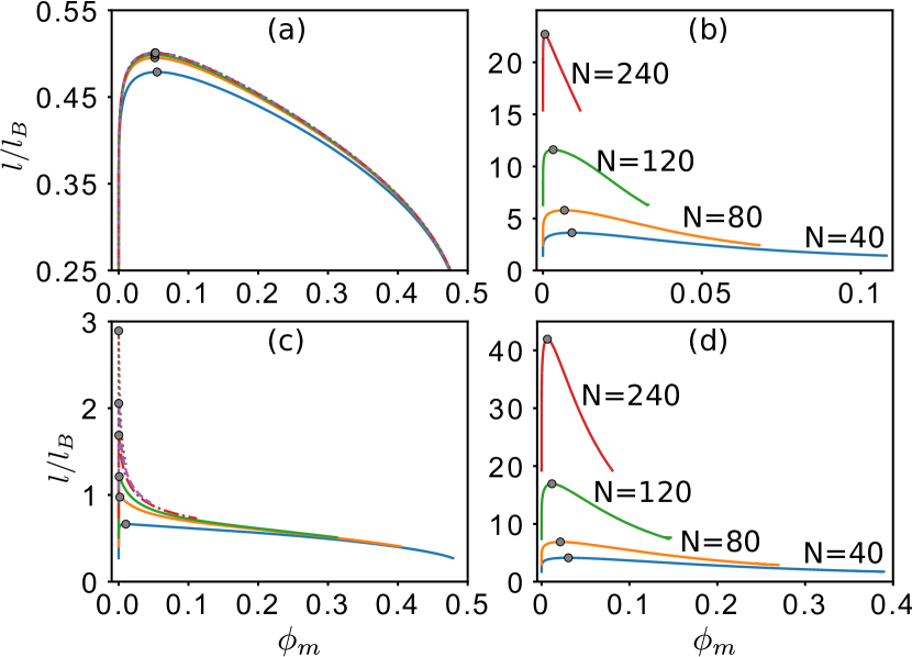
Figure 1: Salt-free LLPS of polyelectrolytes and polyampholytes. rG-RPA (a and b, top panels) and fG-RPA (c and d, bottom panels) phase diagrams for $N=$ 10, 25, 40, 80, 120, and 240 polyelectrolytes with charge sequences $\sigma_{\tau}=-1$ for $\tau=1,2,\dots,N$ (a and c, left panels) and $N=40$, $80$, $120$, and $240$ 4-block polyampholytes with charge sequences $\sigma_{\tau}=+1$ for $\tau=1,2,\dots,N/4$ and $\tau=N/2+1,N/2+2,\dots,3N/4$, and $\sigma_{\tau}=-1$ for $\tau=N/4+1,N/4+2,\dots,N/2$ and $\tau=3N/4+1,3N/4+2,\dots,N$ (b and d, right panels). Grey circles are critical points. For the coexistence curves in (a and c), $N$ decreases from top to bottom, with the $N=$ 80, 120, and 240 curves in (a) being nearly identical.

The rG-RPA-predicted critical point $((\phi_{m})_{\rm cr},1/(l_{\!B})_{\rm cr})$ in Fig. 1(a) for polyelectrolytes is insensitive to chain length ($(l_{\!B})_{\rm cr}$ is critical Bjerrum length; $1/(l_{\!B})_{\rm cr}$ is proportional to the critical temperature $T_{\rm cr}$). As $N$ increases, $\lim_{N\to\infty}1/(l_{\!B})_{\rm cr}\approx 0.5$ and $\lim_{N\to\infty}(\phi_{m})_{\rm cr}\approx 0.05$. These predictions are consistent with lattice-chain simulations Orkoulas, Kumar, and Panagiotopoulos (2003) and other theories Jiang et al. (2001); Muthukumar (2002); Budkov et al. (2015); Shen and Wang (2017). The fG-RPA predictions are drastically different, viz., $\lim_{N\to\infty}1/(l_{\!B})_{\rm cr}\rightarrow\infty$ and $\lim_{N\to\infty}(\phi_{m})_{\rm cr}\rightarrow 0$ (Fig. 1(c)). Thus, fG-RPA is limited as earlier RPA theories Mahdi and Olvera de la Cruz (2000); Ermoshkin and Olvera de la Cruz (2003) and its predictions for polyelectrolytes are inconsistent with the aforementioned established results Jiang et al. (2001); Muthukumar (2002); Orkoulas, Kumar, and Panagiotopoulos (2003); Budkov et al. (2015); Shen and Wang (2017). This comparison between rG-RPA and fG-RPA underscores the importance of appropriately accounting for conformational heterogeneity in understanding polyelectrolyte LLPS and the effectiveness of using renormalized Kuhn lengths for the purpose.

Both rG-RPA and fG-RPA predict $1/(l_{\!B})_{\rm cr}\rightarrow\infty$ and $(\phi_{m})_{\rm cr}\rightarrow 0$ as $N\rightarrow\infty$ for the polyampholytes (Fig. 1(b and d)). These results are consistent with simple RPA theory Lin, Forman-Kay, and Chan (2016); Lin et al. (2017a), a charged hard-sphere chain model Jiang et al. (2006), and lattice-chain simulations Cheong and Panagiotopoulos (2005). Not surprisingly, both rG-RPA and fG-RPA posit that the $T_{\rm cr}$’s of polyelectrolytes are much lower than those of neutral polyampholytes because direct electrostatic attractions exist for polyampholytes but effective attractions among polyelectrolytes can only be mediated by counterions.

For the polyampholytes, rG-RPA (Fig. 1(b)) predicts lower $T_{\rm cr}$’s than fG-RPA (Fig. 1(d)). With a more accurate treatment of single-chain conformational dimensions, rG-RPA should entail more compact isolated single-chain conformations for block polyampholytes, resulting in less accessibility of the charges for interchain cohesive interactions and therefore a weaker—but physically more accurate—LLPS propensity.

Notably, the fG-RPA-predicted phase boundaries of both polyelectrolytes and polyampholytes exhibit an inverse S-shape phase boundaries (the condensed-phase part of the coexistence curves concave upward; Fig. 1(c and d)). In contrast, rG-RPA predicts that only polyampholytes have inverse S-shape phase boundaries (Fig. 1(b)), whereas polyelectrolytes phase boundaries convex upward with a relatively flat $\phi_{m}$ dependence around the critical points (Fig. 1(a)). This conspicuous difference between the rG-RPA-predicted phase boundaries of polyampholytes and polyelectrolytes is consistent with explicit-chain simulations Orkoulas, Kumar, and Panagiotopoulos (2003); Das et al. (2018a).

III.2 Salt-free rG-RPA account of pH-dependent LLPS

To address pH dependence under salt-free conditions, we apply rG-RPA to an example of a near-neutral polyampholyte under neutral pH, namely the N-terminal IDR of the DEAD-box helicase Ddx4 (IDR denoted as Ddx4^N1) and its charge-scrambled variant Ddx4^N1CS which has the same amino acid composition as Ddx4^N1 by a different sequence charge pattern Nott et al. (2015). The sequences are studied at neutral and acidic pH. We refer to the resulting charge patterns as (in obvious notation) $\text{Ddx4}^{\rm N1}_{\rm pH7}$, $\text{Ddx4}^{\rm N1}\text{CS}_{\rm pH7}$, $\text{Ddx4}^{\rm N1}_{\rm pH1}$, and $\text{Ddx4}^{\rm N1}\text{CS}_{\rm pH1}$, where pH7 and pH1 are approximate pH values symbolizing neutral and acidic conditions. For the pH7 sequences, each of the 24 arginines (R) and 8 lysines (K) of Ddx4^N1 and Ddx4^N1CS is assigned a $+1$ charge, each of the 18 aspartic acids (D) and 18 glutamic acids (E) is assigned a $-1$ charge, and the 2 histidines (H) carry zero charge. For the pH1 sequences, because the pH is lower than the pKa of the acidic amino acids (3.71 for D and 4.15 for E), they are not ionized and thus carry zero charge but each K or R or H ($p{\rm K_{H}}=6.04$) carries a $+1$ charge (Fig. 2(a), K, R in blue; H in cyan). Thus, $\text{Ddx4}^{\rm N1}_{\rm pH7}$ and $\text{Ddx4}^{\rm N1}\text{CS}_{\rm pH7}$ are near-neutral polyampholytes whereas $\text{Ddx4}^{\rm N1}_{\rm pH1}$ and $\text{Ddx4}^{\rm N1}\text{CS}_{\rm pH1}$ are polyelectrolytes, although these four sequences—unlike those in Fig. 1—contains also many uncharged monomers.

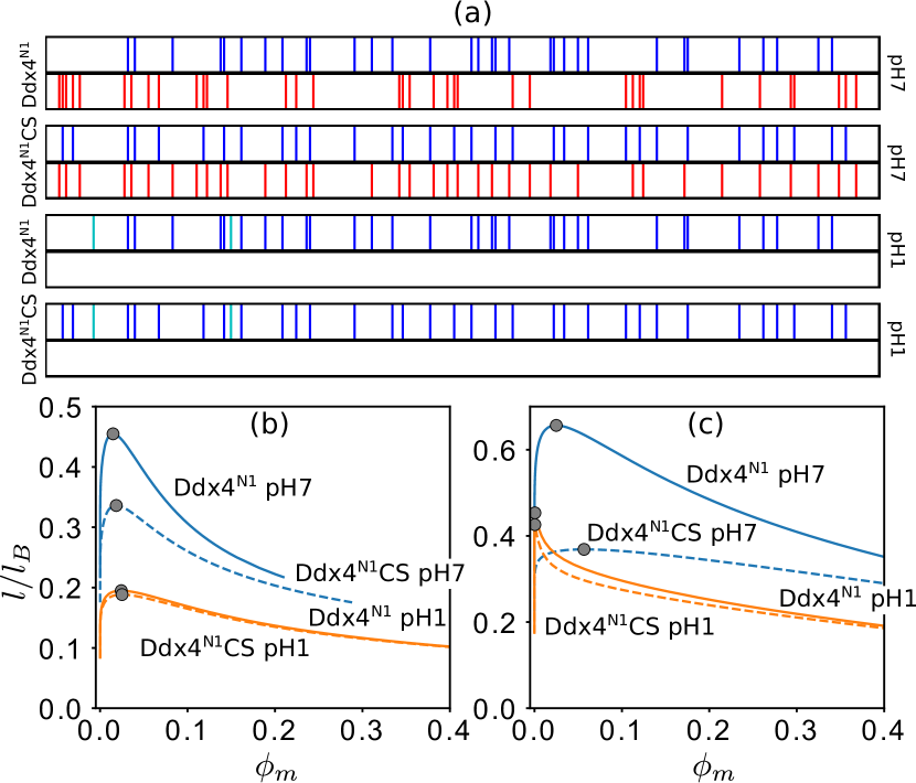
Figure 2: LLPS at neutral and acidic pH. (a) Charge sequences of $\text{Ddx4}^{\rm N1}$ and $\text{Ddx4}^{\rm N1}\text{CS}$ (blue/cyan: $+1$, red: $-1$, white: $0$) and their (b) rG-RPA and (c) fG-RPA phase diagrams.

Fig. 2(b) indicates that the rG-RPA-predicted $T_{\rm cr}$ is much lower under acidic than under neutral conditions, and that the $T_{\rm cr}$ of $\text{Ddx4}^{\rm N1}$ is always higher than that of $\text{Ddx4}^{\rm N1}\text{CS}$ under both pH conditions, underscoring that sequence-specific effects influence the LLPS of not only neutral and nearly-neutral polyampholytes Lin, Forman-Kay, and Chan (2016); Lin et al. (2017a); Lin and Chan (2017); Das et al. (2018b, a) but also polyelectrolytes. Intriguingly, inverse S-shaped coexistence curves are seen in Fig. 2(b) not only for neutral pH (blue curves) but also for acidic pH (orange curves). This feature is characteristic of polyampholytes (Fig. 1(b)) but not uniformly charged polyelectrolytes (Fig. 1(a)). This result suggests that inverse S-shaped phase boundaries can arise in general from a heterogeneous sequence charge pattern because it leads to the simultaneous presence of both attractive and repulsive interchain interactions (which can be counterion-mediated in the case of polyelectrolytes) and therefore allows for condensed-phase configurations with lower densities Das et al. (2018a).

As a control, fG-RPA results are shown in Fig. 2(c). In contrast to rG-RPA, fG-RPA predicts that the $l/(l_{\!B})_{\rm cr}$ value (proportional to $T_{\rm cr}$) of both Ddx4^N1 and Ddx4^N1CS at low pH is higher than that of Ddx4^N1CS at neutral pH, and that the critical volume fractions at low pH are significantly lower than those at neutral pH. Although these differences between fG-RPA and rG-RPA predictions for the Ddx4 IDR remain to be conclusively tested by experiment, the low-pH fG-RPA phase diagrams here (orange curves in Fig. 2(c)) share similar features with the fG-RPA phase diagrams for polyelectrolytes in Fig. 1(c) which, as discussed above, are at odd with trends observed in prior theories and experiments. The fG-RPA results and those obtained using our earlier, simple formulation of RPA Lin, Forman-Kay, and Chan (2016) are very similar (Fig. 3).

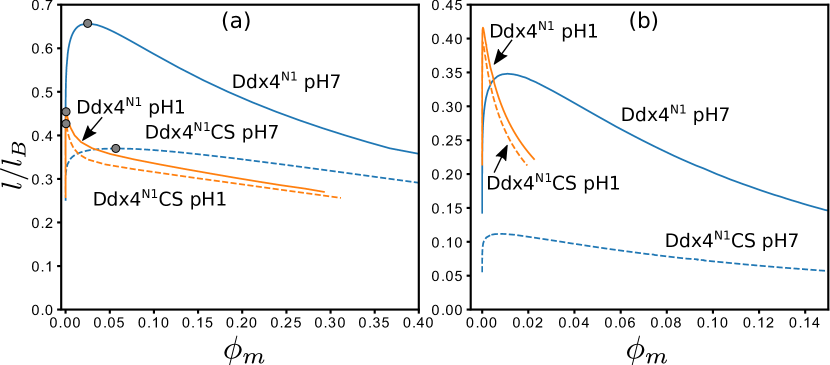
Figure 3: Simple RPA Lin, Forman-Kay, and Chan (2016); Lin et al. (2017a) salt-free phase diagrams for the four Ddx4 sequences in Fig. 2(a). (a) Phase diagrams computed using the Coulomb potential in Fourier space, $U_{k}=4\pi l_{\!B}/k^{2}$, are very similar to the fG-RPA phase diagrams in Fig. 2(c). (b) Phase diagrams computed using a Coulomb potential with a short-range cutoff, $U_{k}=4\pi l_{\!B}/[k^{2}(1+(kl)^{2})]$; the same potential used in our previous simple-RPA studies Lin, Forman-Kay, and Chan (2016); Lin et al. (2017a); Lin and Chan (2017); Lin et al. (2017b); Brady et al. (2017). This Coulomb potential with a short-range cutoff predicts that the two pH1 sequences have critical temperatures even higher than that of wildtype Ddx4 at pH7. This prediction, however, contradicts the physical intuition that polyelectrolytes should have lower phase separation propensities than neutral or near-neutral polyampholytes of the same chain length.

III.3 Salt-free rG-RPA rationalizes pH-dependent LLPS of IP5

We now utilize our theory to rationalize part of the experimental pH-dependent LLPS trend of the lyophilized 39-residue peptide IP5 Wang et al. (2017), the isoelectric point of which is pH = 4.4 (Fig. 4(a and b)) Haynes (2012). The pH-dependent charge $\sigma$ of a basic or acidic residue is computed Ghosh and Dill (2009) here by

$$\sigma=\pm\frac{10^{\pm({\rm pK}_{\rm a}-{\rm pH})}}{1+10^{\pm({\rm pK}_{\rm a}-{\rm pH})}}\;,$$ (18)

where the $+$ and $-$ signs in the $\pm$ signs above apply to the basic (R, K, H) and acidic (D, E) residues, respectively. Standard ${\rm pK}_{\rm a}$ values Haynes (2012), viz., R: $12.10$, K: $10.67$, H: $6.04$, D: $3.71$, and E: $4.15$, are used in Eq. 18 to construct pH-dependent charge sequences of IP5 (Fig. 4(c)).

The rG-RPA- and fG-RPA-predicted IP5 phase boundaries for the experimental studied pH values are shown in Fig. 4(d). Both theories predict a lower $l/(l_{\!B})_{\rm cr}\approx 0.2$–$0.3$ than the experiment $l/(l_{\!B})_{\rm cr}\approx 0.5$. Physically, this is not surprising, as has been addressed in previous RPA studies Lin, Forman-Kay, and Chan (2016), because non-electrostatic cohesive interactions are neglected here. Nonetheless, consistent with experiment, both theories posit that LLPS propensity decreases with increasing pH. Moreover, the rG-RPA-predicted critical volume fraction $(\phi_{m})_{\rm cr}\approx 0.020$–$0.024$ is reasonable in view of the experimental value of $\approx 0.036$ (Ref. (80)), indicating once again that rG-RPA is superior to fG-RPA as the latter predicts much higher $(\phi_{m})_{\rm cr}$’s.

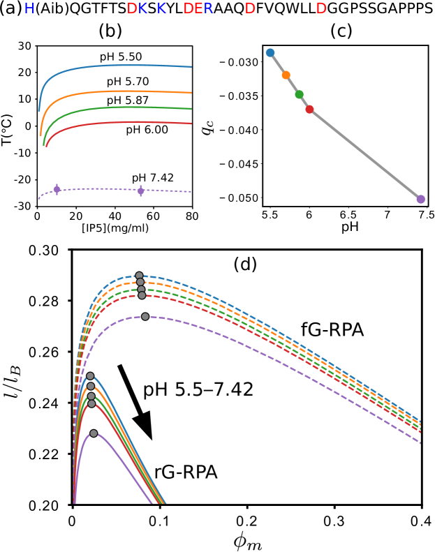
Figure 4: LLPS of IP5. (a) The IP5 sequence, where basic and acidic residues are in blue and red, respectively; (Aib) is the non-proteinogenic amino acid $\alpha$-methylalanine Wang et al. (2017). (b) Experimental pH-dependent phase diagrams of IP5 based on the data in Fig. 4 of Ref. (80); anti-freeze was used to obtain some of the low-$T$ results Wang et al. (2017). (c) Net charge per residue, $q_{c}$, of IP5. (d) Phase diagrams predicted by rG-RPA (solid curves) and fg-RPA (dashed curves).

III.4 Salt-dependent rG-RPA for heteropolymeric charge sequences

In view of the superiority of rG-RPA over fG-RPA, only rG-RPA is used below. We consider the four charge sequences in Fig 2(a) as examples and restrict attention to monovalent salt and counterions ($z_{s}=z_{c}=1$). In experiments we conducted for this study using described methods Brady et al. (2017), no Ddx4^N1 LLPS was observed in salt-free solution at room temperature; yet Ddx4^N1 at room temperature is known Nott et al. (2015); Brady et al. (2017) to phase separate with 100 mM NaCl and that LLPS propensity decreases when [NaCl] is increased to 300 mM. These findings suggest that, similar to LLPS of uniformly charged polyelectrolytes Eisenberg and Mohan (1959); Sabbagh and Delsanti (2000); Prabhu et al. (2001), salt dependence of heteropolymer LLPS is non-monotonic at temperatures slightly higher than the salt-free $T_{\rm cr}$ and therefore such temperatures are of particular interest. For this reason, we apply rG-RPA to compute IDR-salt binary phase diagrams of $\text{Ddx4}^{\rm N1}_{\rm pH7}$, $\text{Ddx4}^{\rm N1}\text{CS}_{\rm pH7}$, $\text{Ddx4}^{\rm N1}_{\rm pH1}$, and $\text{Ddx4}^{\rm N1}\text{CS}_{\rm pH1}$ (Fig. 5), each at an $l/l_{\!B}$ value slightly higher than the sequence’s salt-free $l/(l_{\!B})_{\rm cr}$ in Fig 2(b).

As expected, all binary phase diagrams in Fig. 5 exhibit non-monotonic salt dependence. In general, at temperatures above the salt free critical temperature, i.e. $l/l_{\!B}\gtrsim$ salt-free $l/(l_{\!B})_{\rm cr}$, when sufficient salt is added to the salt-free homogeneous solution, LLPS is triggered at $\phi_{s}=(\phi_{s})^{\rm L}_{\rm cr}$. Adding more salt beyond $(\phi_{s})^{\rm L}_{\rm cr}$ enhances LLPS in that a wider range of overall $\phi_{m}$ falls within the LLPS regime, until a turning point $(\phi_{s})^{\rm T}$ is reached. Beyond that, adding more salt (increasing $\phi_{s}$ above $(\phi_{s})^{\rm T}$) reduces LLPS (the phase-separated range of $\phi_{m}$ narrows). LLPS is impossible for the given temperature when salt concentration is increased above an upper critical point $(\phi_{s})^{\rm U}_{\rm cr}$.

Despite these qualitative commonalities, there are significant sequence-dependent differences. Notably, at neutral pH, the range of salt concentrations that can induce LLPS is much narrower for $\text{Ddx4}^{\rm N1}_{\rm pH7}$ ($\phi_{s}\lesssim 0.00085$, Fig. 5(a)) than for $\text{Ddx4}^{\rm N1}\text{CS}_{\rm pH7}$ ($\phi_{s}\lesssim 0.005$, Fig. 5(b)). However, the ranges of LLPS-inducing salt concentrations at low pH for $\text{Ddx4}^{\rm N1}_{\rm pH1}$ and $\text{Ddx4}^{\rm N1}\text{CS}_{\rm pH1}$ are similar ($\phi_{s}\lesssim 0.01$, Fig. 5(c and d)), and their $(\phi_{s})^{\rm L}_{\rm cr}$ and $(\phi_{s})^{\rm U}_{\rm cr}$ are significantly larger than those at neutral pH.

Next we explore these trends at temperatures below the salt-free $T_{\rm cr}$. Figs. 6–9 present salt-polymer phase diagrams for four Ddx4 sequences (both wild type and charge scrambled sequences at neutral and acidic pH) at three different temperatures. Panels (a) and (b) in these figures show phase diagrams at temperatures below the respective salt free $T_{\rm cr}$ for the given sequence, while panel (c) is at a temperature above salt free $T_{\rm cr}$. The three phase diagrams are compared in panel (d) for a given sequence. These figures reveal trends for $l/l_{\!B}\gtrsim$ salt-free $l/(l_{\!B})_{\rm cr}$ (above the salt free critical temperature) are largely in line with behaviors at temperatures below the salt-free $T_{\rm cr}$. The only difference is for $l/l_{\!B}<$ salt-free $l/(l_{\!B})_{\rm cr}$, $(\phi_{s})^{\rm L}_{\rm cr}=0$. For $l/l_{\!B}<$ salt-free $l/(l_{\!B})_{\rm cr}$, temperatures for different sequences were chosen such that the maximum $\phi_{m}$ range of LLPS are similar among the sequences (as in Fig. 5). With this choice of temperature constraint, when the IDR-salt phase diagrams for different sequences (Figs. 6–9) are compared, we note that $(\phi_{s})_{\rm cr}^{\rm U}$ and $(\phi_{s})^{\rm T}$ of $\text{Ddx4}^{\rm N1}_{\rm pH7}$ are much smaller than those of $\text{Ddx4}^{\rm N1}\text{CS}_{\rm pH7}$. Furthermore, $(\phi_{s})_{\rm cr}^{\rm U}$, $(\phi_{s})^{\rm T}$ of these two pH7 sequences are much smaller than those of the two pH1 sequences. Thus, we conclude that $\text{Ddx4}^{\rm N1}_{\rm pH7}$ is more sensitive to salt than $\text{Ddx4}^{\rm N1}\text{CS}_{\rm pH7}$, and both are more salt-sensitive than $\text{Ddx4}^{\rm N1}_{\rm pH1}$ and $\text{Ddx4}^{\rm N1}\text{CS}_{\rm pH1}$. Metrics other than $(\phi_{s})^{\rm T}$ can also be used to determine salt sensitivity. For example, the low-$\phi_{m}$ turning point (e.g., at $\phi_{m}\approx 0.006$, $\phi_{s}\approx 0.16$ in Fig. 5(a), unlabeled) with a $\phi_{s}$ value similar to that of $(\phi_{s})^{\rm T}$ may be used to characterize salt sensitivity. The resulting trend is similar to the one gleaned from the turning point, $(\phi_{s})^{\rm T}$.

The existence of a $(\phi_{s})^{\rm L}_{\rm cr}>0$ in Fig. 5(a) is consistent with our experimental observation that Ddx4^N1 does not phase separate with [NaCl] $<$ 15–20 mM at pH 6.5, 25^∘C ($l/l_{\!B}=0.529$), and 5mM Tris. Other predictions of our theory remain to be tested. Of particular interest is the slopes of the tie lines in Fig. 5(a) and (b) that change from negative to positive as $\phi_{s}$ increases, indicating that salt ions and the heteropolymeric IDRs partially exclude each other in low-salt but partially coalesce in high-salt solutions at neutral pH. This intriguing feature was not encountered in solutions of either a single species of uniformly-charged or two species of oppositely-charged homopolymers Moreira and Netz (2001); Zhang et al. (2016); Lytle, Radhakrishna, and Sing (2016); Lytle and Sing (2017); Radhakrishna et al. (2017); Shen and Wang (2018); Li et al. (2018). In contrast, the tie-line slopes in Fig. 5(c) and (d) are all positive, indicating that salt ions and the heteropolymeric IDRs always partially coalesce under acidic conditions.

Figure 5: IDR-salt binary phase diagrams of two Ddx4 variants at low and high pH. Results are for $l/l_{\!B}\gtrsim l/(l_{\!B})_{\rm cr}$, where the salt-free $1/(l_{\!B})_{\rm cr}$ equals $0.455$ for $\text{Ddx4}^{\rm N1}_{\rm pH7}$ (a), $0.336$ for $\text{Ddx4}^{\rm N1}\text{CS}_{\rm pH7}$ (b), $0.195$ for $\text{Ddx4}^{\rm N1}_{\rm pH1}$ (c), and $0.188$ for $\text{Ddx4}^{\rm N1}\text{CS}_{\rm pH1}$ (d). The $\phi_{s}$ values of the grey circles in (a)–(d) are $(\phi_{s})_{\rm cr}^{\rm U}$, $(\phi_{s})^{\rm T}$, or $(\phi_{s})_{\rm cr}^{\rm L}$, as indicated by U, T, and L in (a).

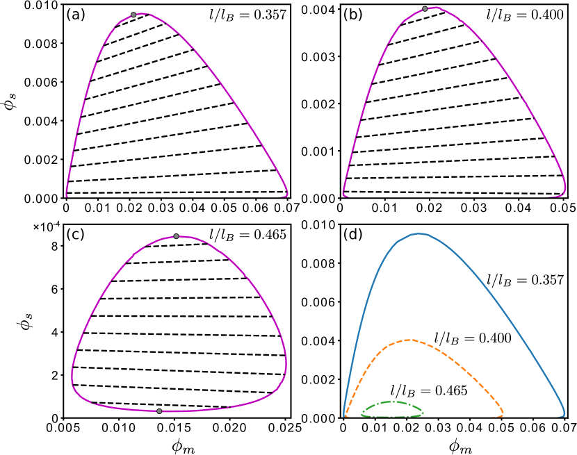
Figure 6: Polymer-salt coexistence phase diagrams of $\text{Ddx4}^{\rm N1}_{\rm pH7}$ at the $l/l_{\!B}$ values indicated. The salt-free critical value of $l/l_{\!B}$ is $l/(l_{\!B})_{\rm cr}=0.455$. Top grey circles in (a), (b), and (c) provide the upper critical salt concentrations $(\phi_{s})^{\rm U}_{\rm cr}$, whereas the bottom grey circle in (c) provides the lower critical concentration $(\phi_{s})^{\rm L}_{\rm cr}$ (see discussion in main text). Each dashed line in (a)–(c) is a tie line connecting a pair of coexistent phases. The three phase boundaries in (a)–(c) are compared in (d).

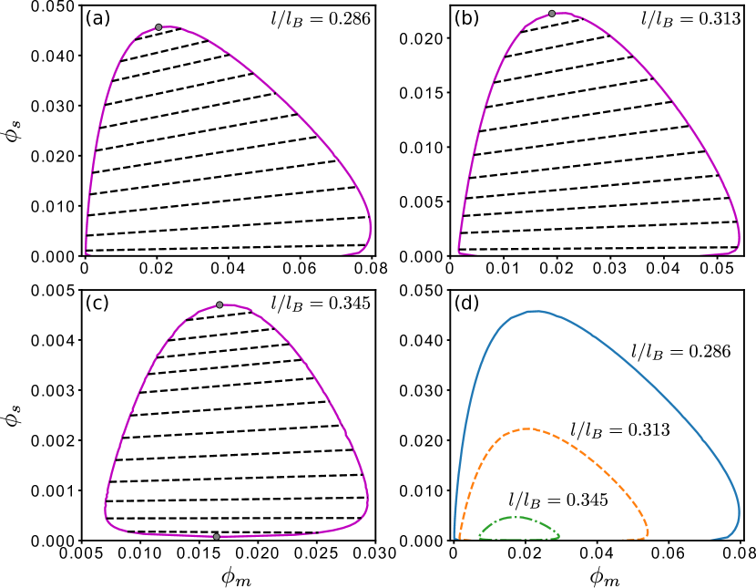
Figure 7: Polymer-salt coexistence phase diagrams of $\text{Ddx4}^{\rm N1}\text{CS}_{\rm pH7}$ at the $l/l_{\!B}$ values indicated. The salt-free critical value of $l/l_{\!B}$ is $l/(l_{\!B})_{\rm cr}=0.336$. Top grey circles in (a), (b), and (c) provide the upper critical salt concentrations $(\phi_{s})^{\rm U}_{\rm cr}$, whereas the bottom grey circle in (c) provides the lower critical concentration $(\phi_{s})^{\rm L}_{\rm cr}$. Each dashed line in (a)–(c) is a tie line connecting a pair of coexistent phases. The three phase boundaries in (a)–(c) are compared in (d).

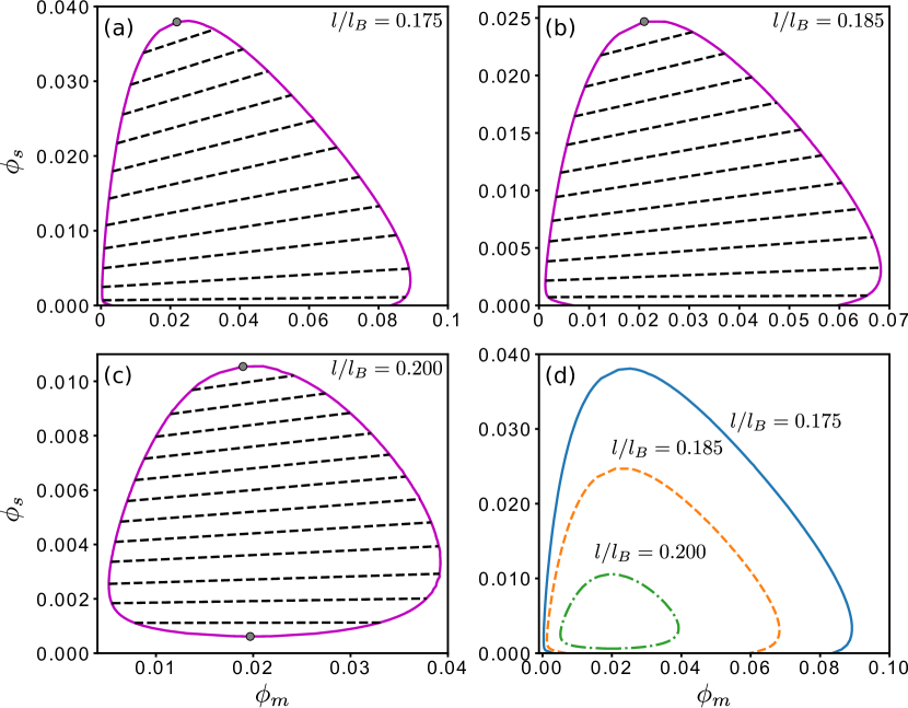
Figure 8: Polymer-salt coexistence phase diagrams of $\text{Ddx4}^{\rm N1}_{\rm pH1}$ at the $l/l_{\!B}$ values indicated. The salt-free critical value of $l/l_{\!B}$ is $l/(l_{\!B})_{\rm cr}=0.195$. Top grey circles in (a), (b), and (c) provide the upper critical salt concentrations $(\phi_{s})^{\rm U}_{\rm cr}$, whereas the bottom grey circle in (c) provides the lower critical concentration $(\phi_{s})^{\rm L}_{\rm cr}$. Each dashed line in (a)–(c) is a tie line connecting a pair of coexistent phases. The three phase boundaries in (a)–(c) are compared in (d).

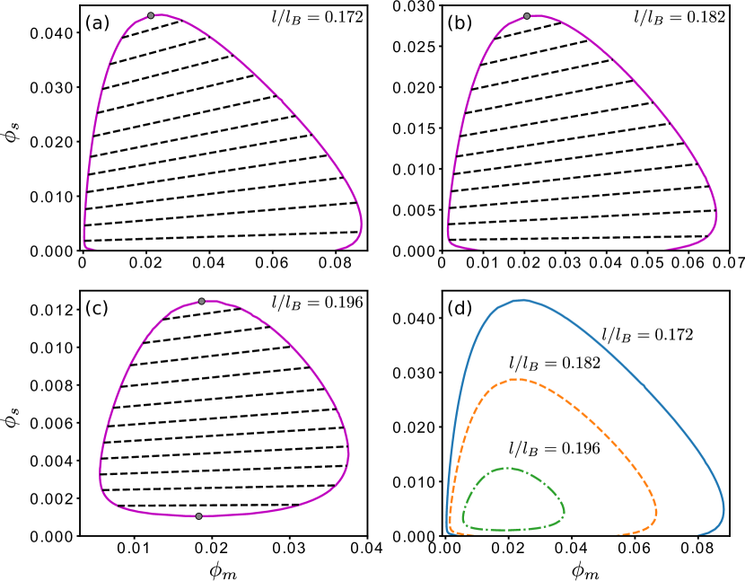
Figure 9: Polymer-salt coexistence phase diagrams of $\text{Ddx4}^{\rm N1}\text{CS}_{\rm pH1}$ at the $l/l_{\!B}$ values indicated. The salt-free critical value of $l/l_{\!B}$ is $l/(l_{\!B})_{\rm cr}=0.188$. Top grey circles in (a), (b), and (c) provide the upper critical salt concentrations $(\phi_{s})^{\rm U}_{\rm cr}$, whereas the bottom grey circle in (c) provides the lower critical concentration $(\phi_{s})^{\rm L}_{\rm cr}$. Each dashed line in (a)–(c) is a tie line connecting a pair of coexistent phases. The three phase boundaries in (a)–(c) are compared in (d).

III.5 Salt-dependent rG-RPA is consistent with established trends in LLPS of homopolymeric, uniformly charged polyelectrolytes

Our model predicts salt and polymers coalesce for $\text{Ddx4}^{\rm N1}_{\rm pH1}$ and $\text{Ddx4}^{\rm N1}\text{CS}_{\rm pH1}$ (Fig. 5 c and d). These sequences are examples of non-uniformly charged polyelectrolytes. However, these results are in contrary to experiment and theory on uniformly charged polyelectrolytes that suggest salt ions and polymers tend to exclude each other, leading to tie lines with negative slopes in the polymer-salt phase diagrams Moreira and Netz (2001); Zhang et al. (2016); Shen and Wang (2018); Eisenberg and Mohan (1959). We test the ability of our model to reproduce this established trend by computing salt-polymer phase diagrams for uniformly charged polymers (Fig. 10(a)). The established feature is captured by our new theory, as the slopes of all tie lines are negative in Fig. 10(a). Furthermore, consistent with literature reports on uniformly charged homopolymers (homopolyelectrolytes) Eisenberg and Mohan (1959); Sabbagh and Delsanti (2000); Prabhu et al. (2001), with addition of salt, rG-RPA predicts a one-to-two phase transition in the low salt regime as well as a two-to-one phase transition in the high salt regime. For comparison, Fig. 10(b) is the phase diagram of an overall neutral polyampholytes at a temperature substantially lower than the salt-free $T_{\rm cr}$ with all tie lines having positive slopes. A recent field theory simulation study of an overall neutral diblock polyampholyte also found tie lines with slightly positive slopes Danielsen et al. (2019b). Since tie lines with exclusively positive slopes are also seen for the overall negatively-charged low-pH Ddx4 IDRs above, the opposite-signed tie-line slopes in Fig. 10(a) for homopolymeric and those in Fig. 5(c) and (d) for heteropolymeric polyelectrolytes suggest a role of sequence heterogeneity in determining whether charged polymers tend to exclude or coalesce with salt ions. However, the precise origins of variation in tie-line slope remains to be ascertained. One idea is that the non-zero tie-line slopes arise from chain connectivity of polymers. If the polymers were not connected and behave like a collections of monomers, the salt concentrations in the dilute and condensed phases would simply follow that of the polymer leading to positive slope Zhang et al. (2018). However chain connectivity can change the slope from positive to negative.

The nature of tie-line slopes has also received considerable attention in the salt-polymer phase diagrams observed during complex coacervation of symmetric polyelectrolytesPerry and Sing (2015); Lytle, Radhakrishna, and Sing (2016); Radhakrishna et al. (2017); Zhang et al. (2018); Adhikari, Leaf, and Muthukumar (2018); Li et al. (2018); Madinya et al. (2019). Insights gleaned from these studies can yield clues to tie-line slope differences observed in our analysis. A recent theory Zhang et al. (2018) based on the concept of chain connectivity predicts a salt-concentration-dependent change of sign of tie-line slope, exhibiting a behavior similar to that in Fig. 5(a) and (b). Although in this case of coacervation the slope changes from positive to negative with addition of salt, opposite to the case of heteropolymers described here. Another idea is that tie-line slope is determined by a competition between electrostatic interactions among polymers and configurational entropy of the salt ions,Adhikari, Leaf, and Muthukumar (2018) whereby the magnitude of electrostatic interactions in the condensed phase are enhanced by reduced salt because of less screening but any difference in concentration in salt ions between the dilute and condensed phases is entropically unfavorable. It is intuitive that both of these proposed mechanisms – conjectured in modeling coacervation – would be affected by the charge pattern of the polymers, but the manner in which the proposed mechanisms are modulated by sequence heterogeneity remains to be investigated.

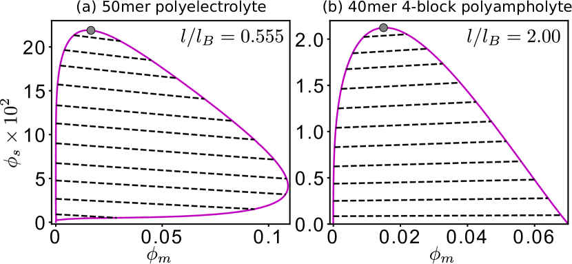
Figure 10: Salt-dependent LLPS of polyelectrolytes and polyampholytes. rG-RPA phase diagrams for (a) an $N=50$ homopolymer with monomer charge $=-1$, and (b) the $N=40$ 4-block polyampholyte in Fig. 1. Note that salt-free $l/(l_{\!B})_{\rm cr}=$ $0.5$ for (a) and $=3.63$ for (b). $(\phi_{s})_{\rm cr}^{\rm U}$ is given by the grey circle. An unmarked $\phi_{s}$ $=(\phi_{s})_{\rm cr}^{\rm L}>0$ exists for (a) but not for (b).

III.6 rG-RPA rationalizes sequence-dependent LLPS of Ddx4 IDRs

Simple RPA theory and an extended RPA+FH theory with an augmented Flory-Huggins (FH) mean-field account of non-electrostatic interactions was utilized to rationalize Lin, Forman-Kay, and Chan (2016); Lin et al. (2017a); Brady et al. (2017) experimental data on sequence- and salt-dependent LLPS of Ddx4 IDRs Nott et al. (2015); Brady et al. (2017). Because RPA accounts only for electrostatic interactions and a sequence-specific analytical treatment of other interactions is currently lacking, FH was used to provide an approximate account of non-electrostatic interactions. These interactions can include hydrophobicity, hydrogen bonding, and especially cation-$\pi$ and $\pi$-$\pi$ interactions because $\pi$-related interactions play prominent roles in LLPS of biomolecular condensates Vernon et al. (2018). To gain further insight into the semi-quantitative picture emerged from these earlier studies Lin, Forman-Kay, and Chan (2016); Lin et al. (2017a); Brady et al. (2017) and to assess the generality of our rG-RPA theory, here we apply an augmented rG-RPA to the LLPS of the same Ddx4^N1 and Ddx4^N1CS sequences by adding to the rG-RPA free energy in Eq. 1 an FH interaction term $-\chi\phi_{m}^{2}$, where $\chi=\Delta H(l_{\!B}/l)-\Delta S$ contains both enthalpic and entropic components, and refer to the resulting formulation as rG-RPA+FH.

To compare with experimental data Brady et al. (2017), we use this theory to compute the phase diagrams of $\text{Ddx4}^{\rm N1}$ and $\text{Ddx4}^{\rm N1}\text{CS}$ at pH 6.5 with 100 and 300ml NaCl, which correspond, respectively, to $\phi_{s}=0.0018$ and 0.0054. Naturally, pH-dependent behaviors can also be obtained by the same FH term together with Eq. 1 and Eq. 18 for rG-RPA free energy; but here we do not pursue a pH-dependent rG-RPA+FH analysis of $\text{Ddx4}^{\rm N1}$ and $\text{Ddx4}^{\rm N1}\text{CS}$ LLPS because no corresponding experimental data is currently available for comparison.

Our detailed rG-RPA study of salt-$\text{Ddx4}^{\rm N1}$ and salt-$\text{Ddx4}^{\rm N1}\text{CS}$ binary phase diagrams in Fig. 5 and Figs. 6–9 indicates that the difference between dilute- and condensed-phase salt concentrations is less than 15% for $\phi_{s}<0.01$. Assuming that this trend is not much affected by non-electrostatic interactions, here we make the simplifying assumption that salt concentration is constant when determining the rG-RPA+FH phase diagrams. Fig. 11(a) shows the resulting rG-RPA+FH theory with $\chi=0.5(l_{\!B}/l)$ fits reasonably well with all four available experimental phase diagrams.

As control, phase diagrams are also computed without the augmented FH term (i.e., $\chi=0$). These phase diagrams are shown as dashed lines in Fig. 11(b). Without the $\chi$ term, the critical temperatures of $\text{Ddx4}^{\rm N1}$ and $\text{Ddx4}^{\rm N1}\text{CS}$ with [NaCl] = 100mM are both predicted to be below 0^∘C (Fig. 11(b)). This theoretical trend is consistent with the experimental observation that phenylalanine to alanine (F-to-A) and arginine to lysine (R-to-K) mutants of $\text{Ddx4}^{\rm N1}$ do not undergo LLPS at physiologically relevant temperatures Nott et al. (2015); Brady et al. (2017); Vernon et al. (2018). These mutations (F-to-A and R-to-K) are expected to significantly reduce $\pi$-related interactions Vernon et al. (2018) and therefore correspond to having a weaker FH term (i.e. $\chi$).

One aforementioned experimentally observed feature that cannot be captured by the present rG-RPA+FH theory is that in the absence of salt, $\text{Ddx4}^{\rm N1}$ at pH 6.5 does not phase separate at room temperature, but rG-RPA+FH with $\chi=0.5(l_{\!B}/l)$ predicts phase separation under the same conditions. There can be multiple reasons for this mismatch between theory and experiment, a likely one of which is that the mean-field treatment of non-electrostatic interactions does not take into possible coupling (cooperative effects) between sequence-specific electrostatic and non-electrostatic interactions such as $\pi$-related interactions and hydrogen bonding that can be enhanced by proximate electrostatic attraction.

Figure 11: Comparing rG-RPA+FH results with experimental data on Ddx4 IDRs. (a) Experimental data of $\text{Ddx4}^{\rm N1}_{\rm pH6.5}$ (wt) and $\text{Ddx4}^{\rm N1}\text{CS}_{\rm pH6.5}$ (cs) (chain length $N=241$ for both sequences) in aqueous solutions with 100 and 300mM NaCl (from Ref. (24); color symbols) are fitted, respectively, to rG-RPA+FH theory with $\phi_{s}=0.0018$ and 0.0054 (continuous curves with the same color). For simplicity, the salt concentrations in the dilute and condensed Ddx4 phases are taken to be identical in this calculation. This is a reasonable approximation because the salt-$\text{Ddx4}^{\rm N1}$ binary phase diagrams in Fig. 5 indicate that the difference in salt concentration between the two phase is less than 15% for $\phi_{s}<0.01$. The fits yield an FH interaction parameter $\chi=0.5(l_{\!B}/l)$ which is equivalent to an enthalpy $\Delta H=-0.56$kcal/mol favorable to polymer-polymer attraction. Model temperatures and model polymer volume fractions are converted, respectively, to ^∘C and mg/ml by a procedure similar to that in Ref. (55) with an appropriately chosen model Kuhn length $l$ that is quite similar to (though not identical with) the C_α–C_α virtual bond length of polypeptides. (b) Phase diagrams of the two sequences with and without the augmented FH interaction. Without the FH term (i.e., $\chi=0$), the critical temperatures of both $\text{Ddx4}^{\rm N1}_{\rm pH6.5}$ and $\text{Ddx4}^{\rm N1}\text{CS}_{\rm pH6.5}$ at 100mM NaCl are below 0^∘C. The two $\chi=0$ systems may be interpreted as corresponding to sequences with reduced favorable non-electrostatic interactions Brady et al. (2017); Vernon et al. (2018). See the main text for further discussion.

IV Conclusions

In summary, we have developed a formalism for salt-, pH-, and sequence-dependent LLPS by combining RPA and Kuhn-length renormalization. The trends predicted by the resulting rG-RPA theory are consistent with established theoretical and experimental results. Importantly, unlike more limited previous analytical approaches, rG-RPA is generally applicable to both polyelectrolytes and neutral/near-neutral polyampholytes. In addition to providing physical rationalizations for experimental data on the pH-dependent LLPS of IP5 peptides and sequence and salt dependence of LLPS of Ddx4 IDRs, our theory offers several intriguing predictions of electrostatics-driven LLPS properties that should inspire further theoretical studies and experimental evaluations. One such observation is that in a salt-heteropolymer system, it is possible for the slope of the tie lines to shift from negative to positive by increasing salt. Although tie lines with exclusively positive or exclusively negative slopes were predicted for uniformly charged polyelectrolytes and diblock polyampholytes Danielsen et al. (2019b); Moreira and Netz (2001); Zhang et al. (2016); Lytle, Radhakrishna, and Sing (2016); Lytle and Sing (2017); Shen and Wang (2018), a salt-dependent change in the sign of tie-line slope for a single species of heteropolymer— specifically from negative to positive with increasing salt—is a notable prediction. In future studies, it would be interesting to explore how this property might have emerged from the intuitively higher degree of sequence heterogeneity of the Ddx4^N1 IDR vis-à-vis that of simple diblock or few-block polyampholytes. In general, the interplay between sequence heterogeneity and a proposed chain connectivity effectZhang et al. (2018) as well as a proposed screening-configurational entropy competition effectAdhikari, Leaf, and Muthukumar (2018) on the salt partitioning slope between dilute and condensed phases remains to be elucidated. Another observation of our work is that inverse S-shape coexistence curves can arise from sequence heterogeneity not only for polyampholytes Lin, Forman-Kay, and Chan (2016); Lin et al. (2017a); Lin and Chan (2017) but also for polyelectrolytes. As emphasized recently Das et al. (2018a), an inverse S-shape coexistence curve allows for a less concentrated condensed phase, which can be of biophysical relevance because it would enable a condensate with higher permeability Wei et al. (2017).

Because rG-RPA is an analytical theory, pertinent numerical computations are much more efficient than field-theory or explicit-chain simulations. Thus, in view of the above advances and despite its approximate nature, rG-RPA should be useful as a high-throughput tool for assessing sequence-dependent LLPS properties in developing basic biophysical understanding and in practical applications such as design of new heteropolymeric materials.

Future development of LLPS theory should address a number of physical properties not tackled by our current theories. These include, but not necessarily limited to: (i) Sequence-dependent effects of non-electrostatic interactions, which is neglected in rG-RPA+FH. (ii) Counterion condensation Manning (1979); Orkoulas, Kumar, and Panagiotopoulos (2003); Muthukumar (2004); Shen and Wang (2018). (iii) Dependence of relative permittivity (dielectric constant) on polymer density Lin et al. (2017a, b) and salt Levy, Andelman, and H (2012). (iv) A more accurate treatment of conformational heterogeneity to compute the structure factor. The present approach accounts approximately for sequence-dependent end-to-end distance, but it fails to capture conformational heterogeneities at smaller length scales Shen and Wang (2018). A formalism for residue-pair-specific renormalized Kuhn length Sawle and Ghosh (2015); Ghosh and Muthukumar (2001) should afford improvement in this regard. (v) Higher-order density fluctuations beyond the quadratic fluctuations Muthukumar (1996) treated by rG-RPA. The rapidly expanding repertoire of experimental data on biomolecular condensates is providing impetus for theoretical efforts in all these directions.

V Acknowledgement

We thank Alaji Bah, Julie Forman-Kay, and Kevin Shen for helpful discussions. This work was supported by Canadian Insitutes of Health Research grant PJT-155930 and Natural Sciences and Engineering Research Council of Canada grant RGPIN-2018-04351 to H.S.C., National Institutes of Health grant 1R15GM128162-01A1 to K.G., and computational resources provided by SciNet of Compute/Calcul Canada. H.S.C. and K.G. are members of the Protein Folding and Dynamics Research Coordination Network funded by National Science Foundation grant MCB 1516959.

Appendix A Derivation of polymer solution free energy

As described in main text, we consider a neutral solution of ${n_{p}}$ charged polymers of $N$ monomers (residues) with charge sequence $|\sigma\rangle=[\sigma_{1},\sigma_{2},...\sigma^{N}]^{\rm T}$. Averaged net charge per monomer is defined as $q_{c}=(\sum_{\tau}\sigma_{\tau})/N$. In addition, there are ${n_{s}}$ salt ions (co-ions) carrying $z_{s}$ charges and ${n_{c}}$ counterions carrying $z_{c}$ charges. Charge neutrality $|q_{c}|{n_{p}}+z_{s}{n_{s}}=z_{c}{n_{c}}$ is always preserved. Monomer and ion densities are defined as $\rho_{m}={n_{p}}N/\Omega$, $\rho_{s}={n_{s}}/\Omega$, and $\rho_{c}={n_{c}}/\Omega$, respectively, with $\Omega$ being the solution volume.

We label the polymers by $\alpha=1,2,\dots,{n_{p}}$ and residues in a polymer by $\tau=1,2,\dots,N$, and denote the spatial coordinate of the $\tau$th monomer in the $\alpha$th polymer by ${\bf R}_{\alpha,\tau}$. Similarly, the small ions are labeled by $a=1,2,\dots,{n_{s}}+{n_{c}}$, in which $1\leq a\leq{n_{s}}$ are for salt ions and ${n_{s}}\!+\!1\leq a\leq{n_{s}}\!+\!{n_{c}}$ are for counterions, with the coordinate of the $a$th small ion denoted by ${\bf r}_{a}$. The implicit-solvent partition function is then expressed as an integral over all solute coordinates divided by factorials that account for the indistinguishability of the molecules within each molecular species in the solution, viz.,

$${\cal Z}=\frac{1}{{n_{p}}!{n_{c}}!{n_{s}}!n_{w}!}\int\prod_{\alpha=1}^{{n_{p}}}\prod_{\tau=1}^{N}d{\bf R}_{\alpha,\tau}\prod_{a=1}^{{n_{s}}+{n_{c}}}d{\bf r}_{a}e^{-\mathscr{T}[{\bf R}]-\mathscr{U}[{\bf R},{\bf r}]},$$ (19)

where $n_{w}$ denotes the number of water molecules, $\mathscr{T}$ accounts for chain connectivity of the polymers, and $\mathscr{U}$ accounts for interactions among all solute molecules, $[{\bf R}]$ is shorthand for $[\{{\bf R}_{\alpha,\tau}\}]$ and $[{\bf R},{\bf r}]$ is shorthand for $[\{{\bf R}_{\alpha,\tau}\},\{{\bf r}_{a}\}]$. Connectivity is enforced by a sum of Gaussian potentials sharing the same Kuhn length $l$, which is given by

$$\mathscr{T}[{\bf R}]=\frac{3}{2l^{2}}\sum_{\alpha=1}^{{n_{p}}}\sum_{\tau=1}^{N-1}\left({\bf R}_{\alpha,\tau+1}-{\bf R}_{\alpha,\tau}\right)^{2}\;.$$ (20)

For simplicity, we assume that interactions in $\mathscr{U}$ are all pairwise, in which case it takes the form

$$\mathscr{U}[{\bf R},{\bf r}]= \frac{1}{2}\sum_{\alpha,\beta=1}^{{n_{p}}}\sum_{\tau,\mu=1}^{N}{\cal U}_{pp}^{\tau\mu}\!\left({\bf R}_{\alpha,\tau}\!-\!{\bf R}_{\beta,\mu}\right)$$ (21)

$$+\sum_{\alpha=1}^{{n_{p}}}\sum_{\tau=1}^{N}\sum_{a=1}^{{n_{s}}+{n_{c}}}{\cal U}_{ps}^{\tau a}\!\left({\bf R}_{\alpha,\tau}\!-\!{\bf r}_{a}\right)$$

$$+\frac{1}{2}\sum_{a,b=1}^{{n_{s}}+{n_{c}}}{\cal U}_{ss}^{ab}\!\left({\bf r}_{a}\!-\!{\bf r}_{b}\right)\;,$$

where ${\cal U}_{pp}$, ${\cal U}_{ps}$, and ${\cal U}_{ss}$ are, respectively, monomer-monomer, monomer-ion, and ion-ion interaction potentials. It should be noted that although self-interactions, that is, the $(\alpha,\tau)=(\beta,\mu)$ terms for monomers and the $a=b$ terms for small ions, are included in the above summation to facilitate subsequent formal development of a field-theory description, these divergent terms will be regularized in the final free energy expression and thus have no bearing on the outcome of our theory. By introducing

$$\rho^{\tau}_{\bf k}= \sum_{\alpha=1}^{{n_{p}}}e^{i{\bf k}\cdot{\bf R}_{\alpha,\tau}}\;,$$ (22a)

$$c^{s}_{\bf k}= \sum_{a=1}^{{n_{s}}}e^{i{\bf k}\cdot{\bf r}_{a}}\;,$$ (22b)

$$c^{c}_{\bf k}= \sum_{a=1}^{{n_{c}}}e^{i{\bf k}\cdot{\bf r}_{a+{n_{s}}}}\;,$$ (22c)

as the ${\bf k}$-space density operators for the monomers and small ions, we rewrite Eq. 21 in ${\bf k}$-space as

$$\mathscr{U}=\frac{1}{2\Omega}\sum_{\bf k}\Bigg{[}\sum_{\tau,\mu=1}^{N}\rho^{\tau}_{\bf k}{\cal U}_{pp}^{\tau\mu}({\bf k})\rho^{\mu}_{-{\bf k}}+2\sum_{\tau=1}^{N}\sum_{\gamma=s,c}\rho^{\tau}_{\bf k}{\cal U}_{ps}^{\tau\gamma}({\bf k})c^{\gamma}_{-{\bf k}}+\!\!\sum_{\gamma,\gamma^{\prime}=s,c}c^{\gamma}_{\bf k}{\cal U}_{ss}^{\gamma\gamma^{\prime}}({\bf k})c^{\gamma^{\prime}}_{-{\bf k}}\Bigg{]}\;,$$ (23)

where $1/\Omega$ is the standard normalization factor for the Fourier transformation, and the general form ${\cal U}({\bf k})=\int d{\bf r}\,{\cal U}({\bf r})\exp(-i{\bf k}\!\cdot\!{\bf r})$ represents the interaction potentials in ${\bf k}$-space. As in Eq. 21 for $\mathscr{U}[{\bf R},{\bf r}]$, the superscripts of ${\cal U}({\bf k})$ are labels for monomers and ions, and the subscripts specify the interaction type. We further define interaction matrices $\hat{{\cal U}}({\bf k})$’s by equating the matrix elements $[\hat{{\cal U}}({\bf k})]_{\tau\mu}$ with ${\cal U}^{\tau\mu}({\bf k})$ for ${\cal U}_{pp}$, ${\cal U}_{ps}$, and ${\cal U}_{ss}$. We also define the density operator vectors $|\rho_{\bf k}\rangle$ and $|c_{\bf k}\rangle$ such that $(|\rho_{\bf k}\rangle)_{\tau}=\rho^{\tau}_{\bf k}$ and $|c_{\bf k}\rangle=[c_{\bf k}^{s},c_{\bf k}^{c}]^{\rm T}$. $\mathscr{U}$ can then be expressed in matrix representation as

$$\mathscr{U}=\frac{1}{2\Omega}\sum_{\bf k}\Bigg{[}\langle\rho_{-{\bf k}}|\hat{{\cal U}}_{pp}({\bf k})|\rho_{{\bf k}}\rangle+2\langle\rho_{-{\bf k}}|\hat{{\cal U}}_{ps}({\bf k})|c_{{\bf k}}\rangle+\langle c_{-{\bf k}}|\hat{{\cal U}}_{ss}({\bf k})|c_{{\bf k}}\rangle\Bigg{]}\;.$$ (24)

The present study foucses on solution systems in which $\mathscr{U}_{ss}$ and $\mathscr{U}_{ps}$ are purely Coulombic whereas $\mathscr{U}_{pp}$ has both Coulombic and pairwise (two-body) excluded-volume repulsion components. Hence

$$\hat{{\cal U}}_{ss}({\bf k})= \frac{4\pi l_{\!B}}{k^{2}}|z\rangle\langle z|\;,$$ (25a)

$$\hat{{\cal U}}_{ps}({\bf k})= \frac{4\pi l_{\!B}}{k^{2}}|\sigma\rangle\langle z|\;,$$ (25b)

$$\hat{{\cal U}}_{pp}({\bf k})= \frac{4\pi l_{\!B}}{k^{2}}|\sigma\rangle\langle\sigma|+v_{2}|1_{N}\rangle\langle 1_{N}|\;,$$ (25c)

where $k\equiv|{\bf k}|$, $l_{\!B}\equiv e^{2}/(4\pi\epsilon k_{\rm B}T)$ is Bjerrum length ($e$ is electronic charge, $\epsilon$ is permittivity, $k_{\rm B}$ is Boltzmann constant, $T$ is absolute temperature). $\langle z|={\rm sign}(q_{c})[z_{s},-z_{c}]$ is the vector representing the charge valencies (number of electronic charges per ion) of salt ions and counterions, respectively, $v_{2}>0$ is the strength of the two-body excluded volume repulsion between monomers, and $|1_{N}\rangle$ is an $N$-dimensional vector in which every component is 1. All elements in the excluded volume matrix $|1_{N}\rangle\langle 1_{N}|$ take unity value because for simplicity all monomers are taken to be of equal size. Substituting the potentials given by Eq. 25 into the ${\cal U}$ function in Eq. 24 yields

$$\mathscr{U}=\frac{1}{2\Omega}\sum_{{\bf k}\neq{\bf 0}}\lambda_{k}|\langle\sigma|\rho_{{\bf k}}\rangle+\langle z|c_{{\bf k}}\rangle|^{2}+\frac{1}{2\Omega}\sum_{{\bf k}}v_{2}|\langle 1_{N}|\rho_{{\bf k}}\rangle|^{2}\;,$$ (26)

where $\lambda_{k}=4\pi l_{\!B}/k^{2}$ and $|A_{\bf k}|^{2}\equiv A_{-{\bf k}}A_{\bf k}$ for arbitrary ${\bf k}$-dependent $A_{{\bf k}}$. The first summation does not need to include ${\bf k}={\bf 0}$ because this term is proportional to the overall net charge of the solution and therefore must be zero because of overall electric neutrality of the solution.

A.1 Field theory for polymer solution

The Hubbard-Stratonovich transformation is then applied to linearize the quadratic form $\mathscr{U}$ in Eq. 26 by introducing conjugate fields $\psi_{\bf k}$ for charge density and $\varw_{\bf k}$ for mass density. The partition function ${\cal Z}$ in Eq. 19 can then be rewritten in terms of

$${\cal Z}^{\prime}= \int\prod_{\alpha=1}^{{n_{p}}}\prod_{\tau=1}^{N}d{\bf R}_{\alpha,\tau}\prod_{a=1}^{{n_{s}}+{n_{c}}}d{\bf r}_{a}e^{-\mathscr{T}[{\bf R}]-\mathscr{U}[{\bf R},{\bf r}]}$$ (27)

$$= \exp\left\{-\frac{1}{2\Omega}v_{2}|\langle 1_{N}|\rho_{{\bf k}={\bf 0}}\rangle|^{2}\right\}\prod_{{\bf k}\neq{\bf 0}}\int\!\!\frac{d\psi_{\bf k}d\varw_{\bf k}}{2\pi\Omega\sqrt{\lambda_{k}v_{2}}}\exp\left\{-\frac{1}{2\Omega}\sum_{{\bf k}\neq{\bf 0}}\left[\frac{|\psi_{\bf k}|^{2}}{\lambda_{k}}+\frac{|\varw_{\bf k}|^{2}}{v_{2}}\right]\right\}$$

$$\times\int\!\prod_{\alpha=1}^{{n_{p}}}\prod_{\tau=1}^{N}d{\bf R}_{\alpha,\tau}\!\!\prod_{a=1}^{{n_{s}}+{n_{c}}}d{\bf r}_{a}\exp\Biggl{\{}-\frac{i}{\Omega}\sum_{{\bf k}\neq{\bf 0}}\Big{[}\big{(}\langle\sigma|\rho_{-{\bf k}}\rangle\!+\langle z|c_{-{\bf k}}\rangle\big{)}\psi_{{\bf k}}+\langle 1_{N}|\rho_{-{\bf k}}\rangle\varw_{{\bf k}}\Big{]}$$

$$\hskip 184.9429pt\!-\!\mathscr{T}[\{{\bf R}_{\alpha,\tau}\}]\Biggr{\}}\;,$$

where ${\cal Z}={\cal Z}^{\prime}/({n_{p}}!{n_{c}}!{n_{s}}!n_{w}!)$. The first term in ${\cal Z}^{\prime}$ is merely the ${\bf k}={\bf 0}$ component of $\mathscr{U}$, which by the definition of $\rho_{\bf k}^{\tau}$ is equal to

$${\cal Z}_{0}\equiv\exp\left\{-\frac{1}{2\Omega}v_{2}|\langle 1_{N}|\rho_{{\bf k}={\bf 0}}\rangle|^{2}\right\}=\exp\left\{-\frac{v_{2}(N{n_{p}})^{2}}{2\Omega}\right\}\;.$$ (28)

The remaining terms in ${\cal Z}^{\prime}$ is a field integral of $\psi$ and $\varw$. The first component (the latter part of the second line in Eq. 27) is an exponential of the quadratic self-correlations, and the second term (the third and fourth lines in Eq. 27) is a partition function for the polymers and the small ions under the influence of $\psi$ and $\varw$, which we now symbolize as

$${{\cal Q}_{\rm sol}}[\psi,\varw]\equiv \int\prod_{\alpha=1}^{{n_{p}}}\prod_{\tau=1}^{N}d{\bf R}_{\alpha,\tau}\prod_{a=1}^{{n_{s}}+{n_{c}}}d{\bf r}_{a}$$ (29)

$$\times\exp\left\{-\frac{i}{\Omega}\sum_{{\bf k}\neq{\bf 0}}\Big{[}\big{(}\langle\sigma|\rho_{-{\bf k}}\rangle\!+\langle z|c_{-{\bf k}}\rangle\big{)}\psi_{{\bf k}}+\langle 1_{N}|\rho_{-{\bf k}}\rangle\varw_{{\bf k}}\Big{]}\!-\!\mathscr{T}[\{{\bf R}_{\alpha,\tau}\}]\right\}\;.$$

By the definitions of $c_{\bf k}$ and $\rho^{\tau}_{\bf k}$ in Eq. 22, the exponent in the integrand of ${{\cal Q}_{\rm sol}}$ may be expressed as

$$-\frac{i}{\Omega}\sum_{{\bf k}\neq{\bf 0}} \Big{[}\big{(}\langle\sigma|\rho_{-{\bf k}}\rangle\!+\langle z|c_{-{\bf k}}\rangle\big{)}\psi_{{\bf k}}+\langle 1_{N}|\rho_{-{\bf k}}\rangle\varw_{{\bf k}}\Big{]}\!-\!\mathscr{T}[\{{\bf R}_{\alpha,\tau}\}]$$ (30)

$$= -\frac{i}{\Omega}\sum_{{\bf k}\neq{\bf 0}}\psi_{\bf k}\left[(|z\rangle)_{s}\sum_{i=a}^{{n_{s}}}e^{-i{\bf k}\cdot{\bf r}_{a}}+(|z\rangle)_{c}\sum_{a={n_{s}}+1}^{{n_{s}}+{n_{c}}}e^{-i{\bf k}\cdot{\bf r}_{a}}\right]$$

$$\quad-\sum_{\alpha=1}^{n_{p}}\left[\frac{3}{2l^{2}}\sum_{\tau=1}^{N-1}\left({\bf R}_{\alpha,\tau+1}-{\bf R}_{\alpha,\tau}\right)^{2}+\frac{i}{\Omega}\sum_{{\bf k}\neq{\bf 0}}\sum_{\tau=1}^{N}\big{(}\sigma_{\tau}\psi_{\bf k}+\varw_{\bf k}\big{)}e^{-i{\bf k}\cdot{\bf R}_{\alpha,\tau}}\right]\;,$$

where $|z\rangle_{s}={\rm sign}(q_{c})z_{s}$ for salt ions and $|z\rangle_{c}=-{\rm sign}(q_{c})z_{c}$ for counterions as defined above. The coordinates of individual small ions and polymers are decoupled in this expression. Thus, the coordinate integrals in ${{\cal Q}_{\rm sol}}$ are also decoupled, allowing it to be written as

$${{\cal Q}_{\rm sol}}[\psi,\varw]=({\cal Q}_{s}[\psi])^{n_{s}}({\cal Q}_{c}[\psi])^{n_{c}}({\cal Q}_{p}[\psi,\varw])^{n_{p}}\;,$$ (31)

where the ${n_{s}}$, ${n_{c}}$, and ${n_{p}}$ superscripts are powers, with ${\cal Q}_{s}$ and ${\cal Q}_{c}$ being the single-molecule partition functions for salt ions and counterions, respectively; $[\psi]$ is shorthand for $[\{\psi_{\bf k}\}]$ and $[\psi,\varw]$ is shorthand for $[\{\psi_{\bf k}\},\{\varw_{\bf k}\}]$. These single-molecule small-ion partition functions are given by

$${\cal Q}_{s,c}[\psi]=\int d{\bf r}_{s,c}\exp\left\{-\frac{i(|z\rangle)_{s,c}}{\Omega}\sum_{{\bf k}\neq{\bf 0}}\psi_{\bf k}e^{-i{\bf k}\cdot{\bf r}_{s,c}}\right\}\;,$$ (32)

where the expression for ${\cal Q}_{s}$ or ${\cal Q}_{c}$ corresponds, respectively, to choosing the subscript “$s$” or $``c$” for the “$s,c$” notation in the above Eq. 32. The single-polymer partition function ${\cal Q}_{p}$ in Eq. 31 equals

$${\cal Q}_{p}[\psi,\varw]=\int\mathscr{D}[{\bf R}]e^{-{\cal H}_{p}[{\bf R};\psi,\varw]}\;,$$ (33)

where $\mathscr{D}[{\bf R}]\equiv\prod_{\tau=1}^{N}d{\bf R}_{\tau}$, $[{\bf R};\psi,\varw]$ is shorthand for $[\{{\bf R}_{\tau}\},\{\psi_{\bf k}\},\{\varw_{\bf k}\}]$, and

$${\cal H}_{p}[{\bf R};\psi,\varw]=\frac{3}{2l^{2}}\sum_{\tau=1}^{N-1}\left({\bf R}_{\tau+1}-{\bf R}_{\tau}\right)^{2}+\frac{i}{\Omega}\sum_{{\bf k}\neq{\bf 0}}\sum_{\tau=1}^{N}(\sigma_{\tau}\psi_{\bf k}+\varw_{\bf k})e^{-i{\bf k}\cdot{\bf R}_{\tau}}\;.$$ (34)

It should be noted that the small-ion label $a$ and the polymer label $\alpha$ are not needed in the single-molecule partition functions in Eqs. 32 and 33. Collecting results from Eqs. 27, 28 and 31 yields the following formula for ${\cal Z}^{\prime}$:

$${\cal Z}^{\prime}={\cal Z}_{0}\int\prod_{{\bf k}\neq{\bf 0}}\frac{d\psi_{\bf k}d\varw_{\bf k}}{2\pi\Omega\sqrt{\lambda_{k}v_{2}}}\exp\left\{-\frac{1}{2\Omega}\sum_{{\bf k}\neq{\bf 0}}\left[\frac{|\psi_{\bf k}|^{2}}{\lambda_{k}}+\frac{|\varw_{\bf k}|^{2}}{v_{2}}\right]\!+\!{n_{s}}\ln{\cal Q}_{s}\!+\!{n_{c}}\ln{\cal Q}_{c}\!+\!{n_{p}}\ln{\cal Q}_{p}\right\}\;,$$ (35)

where ${\cal Z}_{0}$ is provided by Eqs. 28, ${\cal Q}_{s}$, ${\cal Q}_{c}$, and ${\cal Q}_{p}$ are given by Eqs. 32–34.

A.2 Fluctuation expansion of partition function

To evaluate Eq. 35 analytically, we first derive a mean-field solution at $(\psi,\varw)=({\overline{\psi}},{\overline{\varw}})$ in which the mean conjugated fields ${\overline{\psi}}$ and ${\overline{\varw}}$ satisfy the extremum condition $(\delta{\cal Z}^{\prime}/\delta\psi_{\bf k})=(\delta{\cal Z}^{\prime}/\delta\varw_{\bf k})=0$, which leads to the equalities

$$\frac{{\overline{\psi}}_{\bf k}}{\Omega\lambda_{k}}= \frac{{n_{s}}}{{\cal Q}_{s}}\left(\frac{\delta{\cal Q}_{s}}{\delta\psi_{\bf k}}\right)_{({\overline{\psi}},{\overline{\varw}})}+\frac{{n_{c}}}{{\cal Q}_{c}}\left(\frac{\delta{\cal Q}_{c}}{\delta\psi_{\bf k}}\right)_{({\overline{\psi}},{\overline{\varw}})}+\frac{{n_{p}}}{{\cal Q}_{p}}\left(\frac{\delta{\cal Q}_{p}}{\delta\psi_{\bf k}}\right)_{({\overline{\psi}},{\overline{\varw}})},$$ (36a)

$$\frac{{\overline{\varw}}_{{\bf k}}}{\Omega v_{2}}= \frac{{n_{p}}}{{\cal Q}_{p}}\left(\frac{\delta{\cal Q}_{p}}{\delta\varw_{\bf k}}\right)_{({\overline{\psi}},{\overline{\varw}})},$$ (36b)

where the subscript $({\overline{\psi}},{\overline{\varw}})$ indicates that the functional (field) derivatives are evaluated at the to-be-solved mean conjugated fields. The $\psi$ and $\varw$ field are conjugates, respectively, to charge density and mass density. By using Eqs. 32–34 and the fact that the averages $\left\langle\cdots\right\rangle_{x}$ over the spatial coordinates of the given molecular species ($x=p$, $s$, or $c$) of ${\bf k}$-space density operators in Eq. 22 are given by $\langle\rho^{\tau}_{\bf k}\rangle_{p}={n_{p}}\langle e^{i{\bf k}\cdot{\bf R}_{\tau}}\rangle_{p}$, $\langle c^{s}_{\bf k}\rangle_{s}={{n_{s}}}\langle e^{i{\bf k}\cdot{\bf r}_{s}}\rangle_{s}$, and $\langle c^{c}_{\bf k}\rangle_{c}={{n_{c}}}\langle e^{i{\bf k}\cdot{\bf r}_{c}}\rangle_{c}$ because of the decoupling stated above by Eq. 31, the first-order derivatives in Eq. 36 are given by

$$\frac{n_{s,c}}{{\cal Q}_{s,c}}\frac{\delta{\cal Q}_{s,c}}{\delta\psi_{\bf k}}= -\frac{i(|z\rangle)_{s,c}n_{s,c}}{\Omega}\Bigl{(}\left\langle e^{-i{\bf k}\cdot{\bf r}_{s,c}}\right\rangle_{s,c}\Bigr{)}_{(\psi,\varw)}=-\frac{i(|z\rangle)_{s,c}}{\Omega}\Bigl{(}\left\langle c^{s,c}_{-{\bf k}}\right\rangle_{s,c}\Bigr{)}_{(\psi,\varw)}\;,$$ (37a)

$$\frac{{n_{p}}}{{\cal Q}_{p}}\frac{\delta{\cal Q}_{p}}{\delta\psi_{\bf k}}= -\frac{i{n_{p}}}{\Omega}\Biggl{(}\left\langle\sum_{\tau=1}^{N}\sigma_{\tau}e^{-i{\bf k}\cdot{\bf R}_{\tau}}\right\rangle_{p}\;\Biggr{)}_{(\psi,\varw)}\!\!=-\frac{i}{\Omega}\sum_{\tau=1}^{N}\sigma_{\tau}\Bigl{(}\left\langle\rho_{-{\bf k}}^{\tau}\right\rangle_{p}\Bigr{)}_{(\psi,\varw)}\;,$$ (37b)

$$\frac{{n_{p}}}{{\cal Q}_{p}}\frac{\delta{\cal Q}_{p}}{\delta\varw_{\bf k}}= -\frac{i{n_{p}}}{\Omega}\Biggl{(}\left\langle\sum_{\tau=1}^{N}e^{-i{\bf k}\cdot{\bf R}_{\tau}}\right\rangle_{p}\;\Biggr{)}_{(\psi,\varw)}\!\!=-\frac{i}{\Omega}\sum_{\tau=1}^{N}\Bigl{(}\left\langle\rho_{-{\bf k}}^{\tau}\right\rangle_{p}\;\Bigr{)}_{(\psi,\varw)}\;,$$ (37c)

where $(\left\langle\cdots\right\rangle_{x})_{(\psi,\varw)}$ denotes averaging over the spatial coordinates of the given molecular species evaluated for any given conjugate field $\psi,\varw$. With Eq. 37, the relations in Eq. 36 for the mean conjugate fields become

$${\overline{\psi}}_{\bf k}=-i\lambda_{k}\Bigl{(}\left\langle\big{[}\langle\sigma|\rho_{-{\bf k}}\rangle+\langle z|c_{-{\bf k}}\rangle\big{]}\right\rangle_{s,c,p}\Bigr{)}_{({\overline{\psi}},{\overline{\varw}})}\;,\quad\quad{\overline{\varw}}_{\bf k}=-iv_{2}\Bigl{(}\left\langle\big{[}\langle 1_{N}|\rho_{-{\bf k}}\rangle\big{]}\right\rangle_{p}\Bigr{)}_{({\overline{\psi}},{\overline{\varw}})}\;,$$ (38)

which can now be solved self-consistently to determine ${\overline{\psi}}_{\bf k}$ and ${\overline{\varw}}_{\bf k}$.

We proceed to obtain an approximate solution by assuming that within regions where the system exists as a single phase, the mass density is rather homogeneous. In that case, the ${\bf k}\neq{\bf 0}$ components of the density operators $\rho^{\tau}_{\bf k}$, $c^{s}_{\bf k}$, and $c^{c}_{\bf k}$ in Eq. 22 are small (approximately zero). It then follows from Eq. 38 that

$${\overline{\psi}}_{\bf k}\approx{\overline{\varw}}_{\bf k}\approx 0\;,\quad\forall{\bf k}\neq{\bf 0}\;.$$ (39)

These considerations imply that the following approximate relations hold for the averaged densities on the right-hand side of Eq. 37:

$$\left\langle c^{s,c}_{-{\bf k}}\right\rangle_{\approx 0}\approx n_{s,c}\delta_{{\bf k},{\bf 0}}\;,\quad\quad\sum_{\tau=1}^{N}\sigma_{\tau}\left\langle\rho_{-{\bf k}}^{\tau}\right\rangle_{\approx 0}\approx q_{c}{n_{p}}N\delta_{{\bf k},{\bf 0}}\;,\quad\quad\sum_{\tau=1}^{N}\left\langle\rho_{-{\bf k}}^{\tau}\right\rangle_{\approx 0}\approx{n_{p}}N\delta_{{\bf k},{\bf 0}}\;,$$ (40)

where the “$\approx 0$” subscript in $\langle\cdots\rangle_{\approx 0}$ signifies that the given average over the $s$, $c$, or $p$ spatial coordinates is evaluated at the conjuagate fields in Eq. 39 for approximate homogeneous densities. Now, to arrive at a definite approximate description, we expand the logarithmic small-ion partition functions around $\psi_{{\bf k}\neq{\bf 0}}=0$ up to $O(\delta\psi^{2})$. Utilizing the expressions for the averaged densities in Eq. 40 and replacing the conjugate field ${\overline{\psi}}_{{\bf k}\neq{\bf 0}}\approx 0$ (Eq. 39) at which the averages are evaluated by $\psi_{{\bf k}\neq{\bf 0}}=0$, we obtain

$$\ln{\cal Q}_{s,c}[\psi]\approx \ln{\cal Q}_{s,c}[\psi_{{\bf k}\neq{\bf 0}}=0]+\sum_{{\bf k}\neq{\bf 0}}\left(\frac{\delta\ln{\cal Q}_{s,c}}{\delta\psi_{\bf k}}\right)_{0}\delta\psi_{\bf k}+\frac{1}{2}\sum_{{\bf k},{\bf k}^{\prime}\neq{\bf 0}}\left(\frac{\delta^{2}\ln{\cal Q}_{s,c}}{\delta\psi_{\bf k}\delta\psi_{{\bf k}^{\prime}}}\right)_{0}\delta\psi_{\bf k}\delta\psi_{{\bf k}^{\prime}}$$ (41)

$$= \ln\Omega-\frac{i|z\rangle_{s,c}}{\Omega}\sum_{{\bf k}\neq{\bf 0}}\left\langle e^{-i{\bf k}\cdot{\bf r}_{s,c}}\right\rangle_{0}\delta\psi_{\bf k}$$

$$\qquad-\frac{z_{s,c}^{2}}{2\Omega^{2}}\sum_{{\bf k},{\bf k}^{\prime}\neq{\bf 0}}\left[\left\langle e^{-i({\bf k}+{\bf k}^{\prime})\cdot{\bf r}_{s,c}}\right\rangle_{0}-\Bigl{\langle}e^{-i{\bf k}\cdot{\bf r}_{s,c}}\Bigr{\rangle}_{0}\left\langle e^{-i{\bf k}^{\prime}\cdot{\bf r}_{s,c}}\right\rangle_{0}\right]\delta\psi_{\bf k}\delta\psi_{{\bf k}^{\prime}}$$

$$= \ln\Omega-\frac{z_{s,c}^{2}}{2\Omega^{2}}\sum_{{\bf k}\neq{\bf 0}}|\psi_{\bf k}|^{2},$$

where the “0” subscript in $(\cdots)_{0}$ indicates that the derivatives are evaluated at $\psi_{{\bf k}\neq{\bf 0}}=0$. Similarly, replacing the “$\approx 0$” subscripts in Eq. 40, here the “0” subscript in $\langle\cdots\rangle_{0}$ indicates that the average is evaluated at $\psi_{{\bf k}\neq{\bf 0}}=0$. In the last line of the above Eq. 41, the expansion variable $\delta\psi_{\bf k}$ is written as $\psi_{\bf k}$ for every term in the $\sum_{{\bf k}\neq{\bf 0}}$ summation because the expansion is around $\psi_{{\bf k}\neq{\bf 0}}=0$. Substituting Eq. 41 for the $\ln{\cal Q}_{s}$ and $\ln{\cal Q}_{c}$ into Eq. 35 yields

$${\cal Z}^{\prime}\approx{\cal Z}_{0}\int\prod_{{\bf k}\neq{\bf 0}}\frac{d\psi_{\bf k}d\varw_{\bf k}}{2\pi\Omega\sqrt{\lambda_{k}v_{2}}}\exp\left\{-\frac{1}{2\Omega}\sum_{{\bf k}\neq{\bf 0}}\left[|\psi_{\bf k}|^{2}\left(\frac{1}{\lambda_{k}}\!+\!z_{s}^{2}\rho_{s}\!+\!z_{c}^{2}\rho_{c}\right)\!+\!\frac{|\varw_{\bf k}|^{2}}{v_{2}}\right]\!+\!{n_{p}}\ln{\cal Q}_{p}+C\right\}\;,$$ (42)

where $C=({n_{s}}+{n_{c}})\ln\Omega$ will be dropped in subsequent consideration because it has no effect on the relative free energies of different configurational states. Let the exponent in Eq. 42 without $C$ be denoted as $-\mathscr{H}$, then $\mathscr{H}$ may be seen as a Hamiltonian of a polymer system:

$$\mathscr{H}[\psi,\varw]=\frac{1}{2\Omega}\sum_{{\bf k}\neq{\bf 0}}\left[\nu_{k}\psi_{-{\bf k}}\psi_{{\bf k}}+\frac{\varw_{-{\bf k}}\varw_{{\bf k}}}{v_{2}}\right]-{n_{p}}\ln{\cal Q}_{p}[\psi,\varw]\;,$$ (43)

where

$$\frac{1}{\nu_{k}}=\frac{1}{1/\lambda_{k}+z_{s}^{2}\rho_{s}+z_{c}^{2}\rho_{c}}\equiv\frac{4\pi l_{\!B}}{k^{2}+\kappa^{2}}$$ (44)

is merely a Fourier-transformed Coulomb potential with screening length $1/\kappa=[4\pi l_{\!B}(z_{s}^{2}\rho_{s}+z_{c}^{2}\rho_{c})]^{-1/2}$. We may now express ${\cal Z}^{\prime}$ as a product of three components, viz.,

$${\cal Z}^{\prime}={\cal Z}_{0}{\cal Z}_{\rm ion}{\cal Z}_{p}^{\prime}\;,$$ (45)

where ${\cal Z}_{0}$ is defined in Eq. 28,

$${\cal Z}_{\rm ion}=\prod_{{\bf k}\neq{\bf 0}}\frac{1}{\sqrt{\nu_{k}\lambda_{k}}}=\prod_{{\bf k}\neq{\bf 0}}\left[1+\frac{\kappa^{2}}{k^{2}}\right]^{-\frac{1}{2}}\;,$$ (46)

and

$${\cal Z}_{p}^{\prime}=\prod_{{\bf k}\neq{\bf 0}}\int\sqrt{\frac{\nu_{k}}{v_{2}}}\frac{d\psi_{\bf k}d\varw_{\bf k}}{2\pi\Omega}e^{-\mathscr{H}[\psi,\varw]}\;.$$ (47)

Accordingly, the complete partition function ${\cal Z}={\cal Z}^{\prime}/({n_{s}}!{n_{c}}!{n_{p}}!n_{w}!)$ provides free energy of the system in units $k_{\rm B}T$ per volume $l^{3}$:

$$f=-\frac{l^{3}}{\Omega}\ln{\cal Z}=-s+f_{\rm ion}+f_{\rm p}+f_{\rm 0}\;,$$ (48)

where

$$-s= \frac{l^{3}}{\Omega}\ln({n_{s}}!{n_{c}}!{n_{p}}!n_{w}!)\;,$$ (49)

$$f_{\rm 0}= -\frac{l^{3}}{\Omega}\ln{\cal Z}_{0}=\frac{v_{2}l^{3}({n_{p}}N)^{2}}{2\Omega^{2}}=\frac{l^{3}}{2}v_{2}\rho_{m}^{2}\;,$$ (50)

$$f_{\rm ion}= -\frac{l^{3}}{\Omega}\ln{\cal Z}_{\rm ion}=\frac{l^{3}}{2}\sum_{{\bf k}\neq{\bf 0}}\ln\left[1+\frac{\kappa^{2}}{k^{2}}\right]=-\frac{(\kappa l)^{3}}{12\pi}+I_{0}\;,$$ (51)

$$f_{\rm p}= -\frac{l^{3}}{\Omega}\ln{\cal Z}_{p}^{\prime}\;.$$ (52)

A.3 Small-ion free energy

The first term of $f_{\rm ion}$ in Eq. 51 is the standard Debye screening energy. The second term of $f_{\rm ion}$, $I_{0}=l^{3}\kappa^{2}k_{\rm max}$, is formally divergent ($k_{\rm max}$ is the maximum $k$ value of the system, corresponding to the smallest length scale in coordinate space; $I_{0}\to\infty$ as $k_{\rm max}\to\infty$) but since it is linearly proportional to ${n_{s}}$ and ${n_{c}}$ (through its dependence on $\kappa^{2}$, see above), this formally divergent term is irrelevant to the relative free energies of different configurational states of the system Muthukumar (1996). As in most analyses, the ${\bf k}$-summation is performed here by replacing it with a continuous integral over ${\bf k}$-space:

$$\frac{1}{\Omega}\sum_{{\bf k}\neq{\bf 0}}\to\int\frac{d^{3}k}{(2\pi)^{3}}\;.$$ (53)

To make our model physically more realistic, however, we follow Muthukumar Muthukumar (2002); Lee and Muthukumar (2009) who treated the charge of each small ion as distributed over a finite volume with a characteristic length scale comparable to the bare Kuhn length $l$ of the polymers. In this treatment, the point-charge expression for $f_{\rm ion}$ in Eq. 51 is replaced by

$$f_{\rm ion}=-\frac{1}{4\pi}\left[\ln(1+\kappa l)-\kappa l+\frac{1}{2}(\kappa l)^{2}\right]\;,$$ (54)

which reduces to $-(\kappa l)^{3}/(12\pi)$ in Eq. 51, as it should, in the limit of $\kappa l\to 0$. In this regard, Eq. 54—which is used for all rG-RPA and fG-RPA applications in the present work—may be viewed as a regularized, more physical version of Eq. 51.

A.4 Polymer free energy

We now proceed to derive an approximate, tractable analytical expression for ${\cal Z}_{p}^{\prime}$ in Eq. 7 in the main text and Eq. 47 by expanding $\ln{\cal Q}_{p}$ (defined in Eqs. 33 and 34) around $\psi_{{\bf k}\neq{\bf 0}}=\varw_{{\bf k}\neq{\bf 0}}=0$, viz.,

$$\ln{\cal Q}_{p}[\psi,\varw]= \ln{\cal Q}_{p}[\psi_{{\bf k}\neq{\bf 0}}\!=\!\varw_{{\bf k}\neq{\bf 0}}\!=\!0]$$ (55)

$$+\sum_{{\bf k}\neq{\bf 0}}\sum_{\tau=1}^{N}\left(\frac{\delta\ln{\cal Q}_{p}}{\delta\varphi^{\tau}_{\bf k}}\right)_{0}\varphi^{\tau}_{\bf k}+\frac{1}{2}\sum_{{\bf k},{\bf k}^{\prime}\neq{\bf 0}}\sum_{\tau,\mu=1}^{N}\left(\frac{\delta^{2}\ln{\cal Q}_{p}}{\delta\varphi^{\tau}_{\bf k}\delta\varphi^{\mu}_{{\bf k}^{\prime}}}\right)_{0}\varphi^{\tau}_{\bf k}\varphi^{\mu}_{{\bf k}^{\prime}}+O(\varphi^{3})$$

$$= \ln\Omega+\frac{3(N\!-\!1)}{2}\ln\left(\frac{2\pi l^{2}}{3}\right)-\frac{1}{2\Omega^{2}}\sum_{{\bf k}\neq{\bf 0}}\sum_{\tau,\mu=1}^{N}\left\langle e^{-i{\bf k}\cdot({\bf R}_{\tau}-{\bf R}_{\mu})}\right\rangle_{0}\varphi_{\bf k}^{\tau}\varphi_{-{\bf k}}^{\mu}+O(\varphi^{3})\;,$$

where $\varphi^{\tau}_{\bf k}=\sigma_{\tau}\psi_{\bf k}+\varw_{\bf k}$ and the first term in the second line vanishes because of Eq. 40. As in Eq. 41, the first two constant terms in the last line of the above equation have no effect on the relative energies of different configurations of the system and therefore will be discarded for our present purpose. The third term in the last line of Eq. 55 is the intrachain monomer-monomer correlation function evaluated at $\psi_{{\bf k}\neq{\bf 0}}=\varw_{{\bf k}\neq{\bf 0}}=0$. This correlation function is equal to that of a Gaussian chain. However, in the presence of intra- and interchain interactions, a Gaussian-chain description of the polymer chains in our system is unsatisfactory, as has been demonstrated by theoretical and experimental studies Dobrynin, Colby, and Rubinstein (2004); Dobrynin and Rubinstein (2005); Das and Pappu (2013); Dignon et al. (2019) showing that polymers with different net charges and heteropolymers with different charge sequences—even when they have the same net charge—can have dramatically different conformational characteristics. Intuitively, this sequence-dependent conformational heterogeneity should apply not only to the case when a polymer chain is isolated but also to situations in which polymer chains are in semidilute solutions. To account for this fundamental property in the monomer-monomer correlation function, we need to include nonzero $\psi_{{\bf k}\neq{\bf 0}}$ and $\varw_{{\bf k}\neq{\bf 0}}$ fluctuations that arise from the higher-order terms in Eq. 55. Accordingly, based on a rationale similar to that advanced in Refs. (59; 71; 72), we replace the monomer-monomer correlation function in Eq. 55 by a correlation function involving arbitrary fields. This development leads to

$$\ln{\cal Q}_{p}[\psi,\varw]\simeq-\frac{N}{2\Omega^{2}}\sum_{{\bf k}\neq{\bf 0}}\left[\xi_{\bf k}\psi_{\bf k}\psi_{-{\bf k}}+g_{\bf k}\varw_{\bf k}\varw_{-{\bf k}}+2\zeta_{\bf k}\varw_{\bf k}\psi_{-{\bf k}}\right]\;,$$ (56)

where $\xi$, $g$, and $\zeta$ are structure factors of mass and charge densities,

$$\xi_{\bf k}= \frac{1}{N}\sum_{\tau,\mu=1}^{N}\sigma_{\tau}\sigma_{\mu}\Bigl{(}\left\langle e^{i{\bf k}\cdot({\bf R}_{\tau}-{\bf R}_{\mu})}\right\rangle_{p}\Bigr{)}_{(\psi,\varw)}\;,$$ (57a)

$$g_{\bf k}= \frac{1}{N}\sum_{\tau,\mu=1}^{N}\Bigl{(}\left\langle e^{i{\bf k}\cdot({\bf R}_{\tau}-{\bf R}_{\mu})}\right\rangle_{p}\Bigr{)}_{(\psi,\varw)}\;,$$ (57b)

$$\zeta_{\bf k}= \frac{1}{N}\sum_{\tau,\mu=1}^{N}\sigma_{\tau}\Bigl{(}\left\langle e^{i{\bf k}\cdot({\bf R}_{\tau}-{\bf R}_{\mu})}\right\rangle_{p}\Bigr{)}_{(\psi,\varw)}\;.$$ (57c)

Substituting Eq. 56 for $\ln{\cal Q}_{p}$ in Eq. 43, we obtain

$$\mathscr{H}[\psi,\varw]= \frac{1}{2\Omega}\sum_{{\bf k}\neq{\bf 0}}\left\langle\psi_{-{\bf k}}\;\varw_{-{\bf k}}\right|\left(\begin{array}[]{cc}\nu_{k}+\rho_{m}\xi_{\bf k}&\rho_{m}\zeta_{\bf k}\\ \rho_{m}\zeta_{\bf k}&v_{2}^{-1}+\rho_{m}g_{\bf k}\end{array}\right)\left|\begin{array}[]{c}\psi_{\bf k}\\ \varw_{\bf k}\end{array}\right\rangle$$ (58)

$$= \frac{1}{2\Omega}\sum_{{\bf k}\neq{\bf 0}}\langle\Psi_{-{\bf k}}|\hat{\Delta}_{\bf k}|\Psi_{\bf k}\rangle\;,$$

where $\langle\Psi_{-{\bf k}}|\equiv\langle\psi_{-{\bf k}}\;\varw_{-{\bf k}}|$, $|\Psi_{\bf k}\rangle=(\langle\Psi_{-{\bf k}}|)^{*{\rm T}}$, and $\hat{\Delta}_{\bf k}$ is the $2\times 2$ matrix in the above equation. Thus, each term in the product given in Eq. 47 can now be evaluated as a Gaussian integral to yield

$${\cal Z}_{p}^{\prime}=\prod_{{\bf k}\neq{\bf 0}}\sqrt{\frac{\nu_{k}}{v_{2}\det\hat{\Delta}_{\bf k}}}\;.$$ (59)

Therefore, by Eqs. 53 and 59, the unit free energy is now formally given by

$$f_{\rm p}=-\frac{l^{3}\ln{\cal Z}_{p}^{\prime}}{\Omega}=\frac{l^{3}}{2}\int\frac{d^{3}k}{(2\pi)^{3}}\ln\left[1+\rho_{m}\left(\frac{\xi_{\bf k}}{\nu_{k}}+v_{2}g_{\bf k}\right)+\frac{v_{2}}{\nu_{k}}\rho_{m}^{2}\left(\xi_{\bf k}g_{\bf k}-\zeta_{\bf k}^{2}\right)\right].$$ (60)

It should be noted, however, that the $k\equiv|{\bf k}|\to\infty$ behavior of the integrand in the above Eq. 60 needs to be regularized. For point particles, the $k\to\infty$ limit of the pairwise correlation function is a Kronecker-$\delta$:

$$\lim_{k\to\infty}\left\langle e^{i{\bf k}\cdot({\bf R}_{\tau}-{\bf R}_{\mu})}\right\rangle_{p}=\delta_{\tau\mu}\;.$$ (61)

Thus, by Eq. 57,

$$\lim_{k\to\infty}\xi_{\bf k}= \frac{1}{N}\sum_{\tau=1}^{N}\sigma_{\tau}^{2}\;,$$ (62a)

$$\lim_{k\to\infty}g_{\bf k}= 1\;,$$ (62b)

$$\lim_{k\to\infty}\zeta_{\bf k}= q_{c}\;.$$ (62c)

Because $\lim_{k\to\infty}(1/\nu_{k})=\lim_{k\to\infty}4\pi l_{\!B}/k^{2}$ and $v_{2}>0$, Eq. 62 indicates that the integral in Eq. 60 has an ultraviolet (large-$k$) divergence. This divergence is physically irrelevant, however, because the integral can be readily regularized by subtracting the unphysical Coulomb self-energy of the charged monomers

$$f_{\rm self}=\frac{\rho_{m}l^{3}}{2N}\int\frac{d^{3}k}{(2\pi)^{3}}\frac{4\pi l_{\!B}}{k^{2}}\sum_{\tau=1}^{N}\sigma_{\tau}^{2}$$ (63)

that was included merely for formulational convenience in the first place. In the same vein as the charge smearing for the small ions (Eq. 54), we also smear the $\delta$-function excluded volume repulsion by a Gaussian Wang (2010); Villet and Fredrickson (2014), viz.,

$$v_{2}\to v_{2}(k)=v_{2}e^{-\frac{1}{6}(kl)^{2}}\;,$$ (64)

and use $v_{2}(k)$ in the integral of Eq. 60 of $f_{\rm p}$ to give a $v_{2}$-regularized $f_{\rm p}[v_{2}(k)]$. The regularized $f_{\rm p}$ resulting from these two procedures is then given by

$$f_{\rm p}[v_{2}(k)]-f_{\rm self}\rightarrow f_{\rm p}\;,$$ (65)

where the last arrow signifies that this regularized version of $f_{\rm p}$ is the one used for our subsequent theoretical development in the present work.

As discussed above, the present separate treatments for small-ions (Eq. 54) and polymers (Eqs. 60 and 65) are needed in our formulation—which expresses the total partition function as a product consisting of separate factors for small ions and polymers (Eq. 46)—such that the polymer part of the partition function can be used to derive an effective Kuhn length. Not surprisingly, in the event that the bare chain length $l$ is used instead of an effective Kuhn length and that the volume of small ions and the volume of the monomers of the polymers becomes negligible ($v_{2}\rightarrow 0$), the free energy expression reduces to that of our simple RPA theory Lin, Forman-Kay, and Chan (2016); Lin et al. (2017a), as can be readily seen in the following. First, when the size of the small ions is assumed to be negligible, their free energy is given by the simple Debye-Hückel expression in Eq. 51 instead of the finite-size expression in Eq. 54. Second, as $v_{2}\rightarrow 0$, all terms involving $v_{2}$ in Eq. 60 vanish. Consequently, the resulting overall electrostatic free energy, denoted here as $f_{\rm el}$, is given by

$$f_{\rm el}=f_{\rm ion}^{\rm(Eq.\ref{eq:-lnZs})}+f_{\rm p}^{\rm(Eq.\ref{eq:fpolySI})}(v_{2}\to 0)=\frac{l^{3}}{2}\int\frac{d^{3}k}{(2\pi)^{3}}\left\{\ln\left[1+\frac{\kappa^{2}}{k^{2}}\right]+\ln\left[1+\rho_{m}\frac{\xi_{\bf k}}{\nu_{k}}\right]\right\}.$$ (66)

Recalling that $\kappa^{2}=4\pi l_{\!B}(z_{s}^{2}\rho_{s}+z_{c}^{2}\rho_{c})$ and $1/\nu_{k}=4\pi l_{\!B}/(k^{2}+\kappa^{2})$ (Eq. 44), this quantity becomes

$$f_{\rm el}= \frac{l^{3}}{2}\int\frac{d^{3}k}{(2\pi)^{3}}\ln\left[\frac{{\kappa^{2}+k^{2}}}{k^{2}}\times\frac{k^{2}+\kappa^{2}+4\pi l_{\!B}\rho_{m}\xi_{\bf k}}{{k^{2}+\kappa^{2}}}\right]$$ (67)

$$= \frac{l^{3}}{2}\int\frac{d^{3}k}{(2\pi)^{3}}\ln\left[1+\frac{\kappa^{2}+4\pi l_{\!B}\rho_{m}\xi_{\bf k}}{k^{2}}\right]$$

$$= \frac{l^{3}}{2}\int\frac{d^{3}k}{(2\pi)^{3}}\ln\left[1+\frac{4\pi l_{\!B}}{k^{2}}\left(z_{s}^{2}\rho_{s}+z_{c}^{2}\rho_{c}^{2}+\rho_{m}\xi_{\bf k}\right)\right],$$

which is exactly the same $f_{\rm el}$ expression in our previous simple RPA theory in a formulation that does not consider an explicit excluded-volume repulsion term and treats small ions and polymers on the same footingLin, Forman-Kay, and Chan (2016); Lin et al. (2017a).

A.5 Effective Gaussian-chain model for two-body correlation function

The $(\psi,\varw)$-dependence of the structure factors $\xi$, $g$, and $\zeta$ in Eq. 60 for $f_{\rm p}$ allows for an account of sequence-dependence conformational heterogeneity by using a Gaussian chain with a renormalized Kuhn length Sawle and Ghosh (2015) $l_{1}=xl$ (instead of the “bare” Kuhn length $l$) to approximate the polymer partition function ${\cal Q}_{p}$ in Eq. 33. Specifically, we make the approximation that

$${\cal Q}_{p}\approx\int\mathscr{D}[{\bf R}]e^{-{\cal H}_{p}^{0}[{\bf R}]}\;,\quad{\rm where}\quad{\cal H}_{p}^{0}[{\bf R}]=\frac{3}{2l^{2}x}\sum_{\tau=1}^{N-1}\left({\bf R}_{\tau+1}-{\bf R}_{\tau}\right)^{2}.$$ (68)

The structure factors $\xi$, $g$, and $\zeta$ in Eq. 57 can then be readily expressed in terms of the yet-to-be-determined renormalization parameter $x$:

$$\xi_{\bf k}\to \xi_{k}^{x}=\frac{1}{N}\sum_{\tau,\mu=1}^{N}\sigma_{\tau}\sigma_{\mu}e^{-\frac{1}{6}(kl)^{2}x|\tau-\mu|}\;,$$ (69a)

$$g_{\bf k}\to g_{k}^{x}=\frac{1}{N}\sum_{\tau,\mu=1}^{N}e^{-\frac{1}{6}(kl)^{2}x|\tau-\mu|}\;,$$ (69b)

$$\zeta_{\bf k}\to \zeta_{k}^{x}=\frac{1}{N}\sum_{\tau,\mu=1}^{N}\sigma_{\tau}e^{-\frac{1}{6}(kl)^{2}x|\tau-\mu|}\;.$$ (69c)

The renormalization parameter $x=l_{1}/l$ is determined using a sequence-specific variational approach introduced by Sawle and Ghosh Sawle and Ghosh (2015); Muthukumar (1987), as follows. We first express the Hamiltonian ${\cal H}_{p}[{\bf R}]$ in Eq. 34 as ${\cal H}_{p}={\cal H}_{p}^{0}+{\cal H}_{p}^{1}$, where ${\cal H}_{p}^{0}$ (given by Eq. 68) is the principal term and

$${\cal H}_{p}^{1}[{\bf R};\psi,\varw]=\frac{3}{2l^{2}}\left(1-\frac{1}{x}\right)\sum_{\tau=1}^{N-1}\left({\bf R}_{\tau+1}-{\bf R}_{\tau}\right)^{2}+\frac{i}{\Omega}\sum_{{\bf k}\neq{\bf 0}}\sum_{\tau=1}^{N}\left(\sigma_{\tau}\psi_{\bf k}+\varw_{\bf k}\right)e^{-i{\bf k}\cdot{\bf R}_{\tau}}\;$$ (70)

is the perturbative term. Then, for any given physical quantity $A[{\bf R}]$, the perturbation expansion of its thermodynamic average over polymer configurations $\{{\bf R}_{\tau}\}$ and field fluctuations $\Psi=(\psi,\varw)$ is given by Doi and Edwards (1986)

$$\langle A[{\bf R}]\rangle= \frac{\left\langle e^{-{\cal H}_{p}^{1}[{\bf R};\Psi]}A[{\bf R}]\right\rangle_{0,\Psi}}{\left\langle e^{-{\cal H}_{p}^{1}[{\bf R};\Psi]}\right\rangle_{0,\Psi}}$$ (71)

$$= \left\langle A[{\bf R}]\right\rangle_{0}+\left[\left\langle A[{\bf R}]\right\rangle_{0}\left\langle{\cal H}_{p}^{1}[{\bf R};\Psi]\right\rangle_{0,\Psi}-\left\langle A[{\bf R}]\,{\cal H}_{p}^{1}[{\bf R};\Psi]\right\rangle_{0,\Psi}\right]$$

$$\qquad\quad\;\;+\frac{1}{2}\left[\left\langle A[{\bf R}]\left({\cal H}_{p}^{1}[{\bf R};\Psi]\right)^{2}\right\rangle_{0,\Psi}-\left\langle A[{\bf R}]\right\rangle_{0}\left\langle\left({\cal H}_{p}^{1}[{\bf R};\Psi]\right)^{2}\right\rangle_{0,\Psi}\right]$$

$$\qquad\quad\;\;+\left\langle A[{\bf R}]\right\rangle_{0}\left\langle{\cal H}_{p}^{1}[{\bf R};\Psi]\right\rangle_{0,\Psi}^{2}-\left\langle A[{\bf R}]{\cal H}_{p}^{1}[{\bf R};\Psi]\right\rangle_{0,\Psi}\left\langle{\cal H}_{p}^{1}[{\bf R};\Psi]\right\rangle_{0,\Psi}$$

$$\qquad\quad\;\;+O\left(({\cal H}_{p}^{1})^{3}\right)\;,$$

where the subscripts $0,\Psi$ in $\left\langle\cdots\right\rangle$ signify, respectively, that the average over $\{{\bf R}_{\tau}\}$’s is weighted by the Hamiltonian ${\cal H}_{p}^{0}[{\bf R}]$ in Eq. 68 and the average over field configurations is weighted by the Hamiltonian $\mathscr{H}[\psi,\varw]$ in Eq. 43. (Note that the meaning of the “0” subscript here is different from that for the averages evaluated at $\psi_{{\bf k}\neq{\bf 0}}=\varw_{{\bf k}\neq{\bf 0}}=0$ in Eq. 41). An ${\cal H}_{p}^{0}[{\bf R}]$ that provides a good description of the thermal properties of $A$ may then be obtained by minimizing $\left\langle A\right\rangle-\left\langle A\right\rangle_{0}$. This is accomplished by a partial optimization to seek a value of $x=l_{1}/l$ that would abolish the lowest-order nontrivial ${\cal H}_{p}^{1}$ contributions in Eq. 71.

To obtain a partially optimized $x=l_{1}/l$ that provides a good approximation for the monomer-monomer correlation function, $A$ is chosen to be the squared end-to-end distance of the polymer, i.e., $A=R_{ee}^{2}\equiv|{\bf R}_{N}-{\bf R}_{1}|^{2}$, because $R_{ee}$ is a simple yet effective measure of conformational dimensions of polymers Muthukumar (1996); Sawle and Ghosh (2015). To facilitate this calculation, we express ${\cal H}_{p}^{1}$ in Eq. 70 as ${\cal H}_{p}^{1}={\cal X}_{1}+{\cal X}_{2}$, where

$${\cal X}_{1}[{\bf R}]= \frac{3}{2l^{2}}\left(1-\frac{1}{x}\right)\sum_{\tau=1}^{N-1}\left({\bf R}_{\tau+1}-{\bf R}_{\tau}\right)^{2}\;,$$ (72a)

$${\cal X}_{2}[{\bf R};\Psi]= \frac{i}{\Omega}\sum_{{\bf k}\neq{\bf 0}}\sum_{\tau=1}^{N}\left(\sigma_{\tau}\psi_{\bf k}+\varw_{\bf k}\right)e^{-i{\bf k}\cdot{\bf R}_{\tau}}\;,$$ (72b)

such that ${\cal X}_{1}[{\bf R}]$ is independent of $\Psi$ and all of ${\cal H}_{p}^{1}$’s dependence on $\Psi$ is contained in ${\cal X}_{2}[{\bf R};\Psi]$. It follows that the $\Psi$ average is trivial (i.e., it produces a multiplicative factor of unity and therefore can be omitted) for any function of ${\cal X}_{1}[{\bf R}]$ only. In Eq. 71, the only contributions from terms linear in ${\cal X}_{1}[{\bf R}]$ come from the first line on the right-hand side (after the second equality), which equal

$$\left\langle R_{ee}^{2}\right\rangle_{0}\left\langle{\cal X}_{1}\right\rangle_{0}-\left\langle R_{ee}^{2}{\cal X}_{1}\right\rangle_{0}=-l^{2}(N-1)x(x-1)\;.$$ (73)

For the ${\cal X}_{2}$-containing terms in Eq. 71, we first consider their $\Psi$-averages before applying the $\left\langle\cdots\right\rangle_{0}$ averaging. For terms linear in ${\cal X}_{2}$, it is straightforward to see that

$$\left\langle{\cal X}_{2}\right\rangle_{\Psi}=\frac{i}{\Omega}\sum_{{\bf k}\neq{\bf 0}}\sum_{\tau=1}^{N}\Big{[}\sigma_{\tau}\left\langle\psi_{\bf k}\right\rangle_{\Psi}+\left\langle\varw_{\bf k}\right\rangle_{\Psi}\Big{]}e^{-i{\bf k}\cdot{\bf R}_{\tau}}=0$$ (74)

because $\left\langle\psi_{\bf k}\right\rangle_{\Psi}=\left\langle\varw_{\bf k}\right\rangle_{\Psi}=0$ according to the quadratic-field Hamiltonian $\mathscr{H}[\psi,\varw]$ in Eq. 58. Thus, ${\cal X}_{2}$ has zero contribution in the first and third lines on the right-hand side of Eq. 71. In contrast, terms quadratic in ${\cal X}_{2}[{\bf R}]$ are not identical zero, because

$$\left\langle{\cal X}_{2}^{2}\right\rangle_{\Psi}=-\frac{1}{\Omega^{2}}\sum_{{\bf k}\neq{\bf 0}}\sum_{\tau,\mu=1}^{N}\Big{[}\sigma_{\tau}\sigma_{\mu}\left\langle\psi_{-{\bf k}}\psi_{{\bf k}}\right\rangle_{\Psi}+\left\langle\varw_{-{\bf k}}\varw_{{\bf k}}\right\rangle_{\Psi}+(\sigma_{\tau}\!+\!\sigma_{\mu})\left\langle\psi_{-{\bf k}}\varw_{{\bf k}}\right\rangle_{\Psi}\Big{]}e^{-i{\bf k}\cdot({\bf R}_{\tau}-{\bf R}_{\mu})}\;,$$ (75)

and here $\left\langle{\cal X}_{2}^{2}\right\rangle_{\Psi}$ is seen as depending on field-field correlation functions $\left\langle\psi\psi\right\rangle$, $\left\langle\varw\varw\right\rangle$, and $\left\langle\psi\varw\right\rangle$ averaged over $\Psi$. Thus, the ${\cal X}_{2}^{2}$ factors in the averages in the second line on the right-hand side of Eq. 71 provide the only nonzero contribution through second order in ${\cal H}_{p}^{1}$. Following Ref. (59), we only consider lowest-order nonzero contributions from ${\cal X}_{1}$, and from ${\cal X}_{2}$, separately, i.e., including only terms through $O({\cal X}_{1})$ and $O({\cal X}_{2}^{2})$ as discussed above. This approach to the perturbative analysis of Eq. 71 may also be rationalized by an alternate analytical formulation put forth in Refs. (71; 72).

As shown in Eq. 58, the field configuration distribution may be approximated by a Gaussian distribution embodied by the quadratic Hamiltonian $\mathscr{H}[\psi,\varw]$. According to perturbation theory Cardy (1996); Lin et al. (2017a), the field-field correlation functions in Eq. 75 can now be obtained from the matrix $\hat{\Delta}_{\bf k}$ in Eq. 58 via the relationships

$$\frac{\left\langle\psi_{-{\bf k}}\psi_{\bf k}\right\rangle}{\Omega}= \left(\hat{\Delta}_{\bf k}^{-1}\right)_{11}=\frac{v_{2}^{-1}+\rho_{m}g_{\bf k}}{\det\hat{\Delta}_{\bf k}}\;,$$ (76a)

$$\frac{\left\langle\varw_{-{\bf k}}\varw_{\bf k}\right\rangle}{\Omega}= \left(\hat{\Delta}_{\bf k}^{-1}\right)_{22}=\frac{\nu_{k}+\rho_{m}\xi_{\bf k}}{\det\hat{\Delta}_{\bf k}}\;,$$ (76b)

$$\frac{\left\langle\psi_{-{\bf k}}\varw_{{\bf k}}\right\rangle}{\Omega}=\frac{\left\langle\psi_{{\bf k}}\varw_{-{\bf k}}\right\rangle}{\Omega}= \left(\hat{\Delta}_{\bf k}^{-1}\right)_{12}=\left(\hat{\Delta}_{\bf k}^{-1}\right)_{21}=\frac{-\rho_{m}\zeta_{\bf k}}{\det\hat{\Delta}_{\bf k}}\;.$$ (76c)

Hence $\left\langle{\cal X}_{2}^{2}\right\rangle$ is expressed in terms of $\hat{\Delta}_{\bf k}$ as

$$\left\langle{\cal X}_{2}^{2}\right\rangle= -\frac{1}{\Omega}\sum_{{\bf k}\neq{\bf 0}}\sum_{\tau,\mu=1}^{N}\frac{\left\langle\sigma_{\tau}\;1\right|\left(\begin{array}[]{cc}v_{2}^{-1}+\rho_{m}g_{\bf k}&-\rho_{m}\zeta_{\bf k}\\ -\rho_{m}\zeta_{\bf k}&\nu_{k}+\rho_{m}\xi_{\bf k}\end{array}\right)\left|\begin{array}[]{c}\sigma_{\mu}\\ 1\end{array}\right\rangle}{\det\hat{\Delta}_{\bf k}}e^{-i{\bf k}\cdot({\bf R}_{\tau}-{\bf R}_{\mu})}\;.$$ (77)

It should be noted that the excluded volume interaction $v_{2}$ is not regularized by Eq. 64 here because a $k$-independent $v_{2}$ is needed to guarantee a real solution for the renormalization parameter $x$ for arbitrary charge sequence $|\sigma\rangle$ (Refs. (68; 69)). Thus, the regularized form of $v_{2}$ in Eq. 64 applies only to the explicit $v_{2}$ dependence of $f_{\rm p}$ in Eq. 60 but not the implicit $v_{2}$ dependence of $x$ contained in the renormalized form of the structure factors $\xi$, $g$, and $\zeta$. Substituting the $x$-dependent correlation functions in Eq. 69 for the structure factors in Eq. 77, we obtain the nonzero contribution from ${\cal X}_{2}$ in the second line of the right-hand side of Eq. 71 as

$$\frac{1}{2}\left[\langle R_{ee}^{2}{\cal X}_{2}^{2}\rangle_{0}-\langle R_{ee}^{2}\rangle_{0}\langle{\cal X}_{2}^{2}\rangle_{0}\right]=\frac{Nl^{4}x^{2}}{18}\int\!\!\frac{d^{3}k}{(2\pi)^{3}}\frac{k^{2}\Xi_{k}^{x}}{\det\Delta_{k}^{x}}\;,$$ (78)

where

$$\det\Delta_{k}^{x}=\frac{\nu_{k}}{v_{2}}+\rho_{m}\left(\frac{\xi_{k}^{x}}{v_{2}}+\nu_{k}g_{k}^{x}\right)+\rho_{m}^{2}\left[\xi_{k}^{x}g_{k}^{x}-\right(\zeta_{k}^{x}\left){}^{2}\right]\;,$$ (79)

and

$$\Xi_{k}^{x}\equiv\frac{\bar{\xi}_{k}^{x}}{v_{2}}+\nu_{k}\bar{g}_{k}^{x}+\rho_{m}\left(\bar{\xi}_{k}^{x}g_{k}^{x}+\xi_{k}^{x}\bar{g}_{k}^{x}-2\zeta_{k}^{x}\bar{\zeta}_{k}^{x}\right)\;.$$ (80)

Here the renormalized $\bar{\xi}$, $\bar{g}$, and $\bar{\zeta}$ are given by

$$\bar{\xi}_{k}^{x}= \frac{1}{N}\sum_{\tau,\mu=1}^{N}\sigma_{\tau}\sigma_{\mu}|\tau-\mu|^{2}e^{-\frac{1}{6}(kl)^{2}x|\tau-\mu|}\;,$$ (81a)

$$\bar{g}_{k}^{x}= \frac{1}{N}\sum_{\tau,\mu=1}^{N}|\tau-\mu|^{2}e^{-\frac{1}{6}(kl)^{2}x|\tau-\mu|}\;,$$ (81b)

$$\bar{\zeta}_{k}^{x}= \frac{1}{N}\sum_{\tau,\mu=1}^{N}\sigma_{\tau}|\tau-\mu|^{2}e^{-\frac{1}{6}(kl)^{2}x|\tau-\mu|}\;.$$ (81c)

Finally, by combining Eqs. 73 and 78, we arrive at the variational equation

$$1-\frac{1}{x}-\frac{Nl^{2}}{18(N-1)}\int\!\!\frac{d^{3}k}{(2\pi)^{3}}\frac{k^{2}\Xi_{k}^{x}}{\det\Delta_{k}^{x}}=0$$ (82)

for solving $x$. In our numerical calculations, we take $v_{2}=4\pi l^{3}/3$. Inserting the solution of $x$ into Eq. 69 provides an improved accounting of the conformational heterogeneity in the free energy; and this improvement is central to the present rG-RPA theory.

A.6 Mixing entropy

The factorials in Eq. 19 arise from the indistinguishability of the molecules belonging to the same species. Taking logarithm and using Stirling’s approximation, one obtains

$$-\frac{S}{k_{\rm B}}= \ln\left({n_{p}}!{n_{s}}!{n_{c}}!n_{\varw}!\right)$$ (83)

$$\simeq {n_{p}}\ln{n_{p}}+{n_{s}}\ln{n_{s}}+{n_{c}}\ln{n_{c}}+n_{w}\ln n_{w}-{n_{p}}-{n_{c}}-{n_{s}}-n_{w}\;,$$

where additive terms of the form $[\ln(2\pi n)]/2$ (where $n={n_{p}}$, ${n_{s}}$, ${n_{c}}$, or $n_{w}$) are omitted because for large $n$, their contributions is negligible in comparison to the terms included in Eq. 83. As in Ref. (56), here we assume for simplicity that the size of a monomer, a small ion, or a water molecule all equals $l^{3}$. Assuming further, for simplicity, that the system is incompressible, i.e., the system volume $\Omega$ is fully occupied by polymers, small ions, and water, then

$$\frac{1}{\Omega}\left(N{n_{p}}+{n_{s}}+{n_{c}}+n_{w}\right)=\rho_{m}+\rho_{s}+\rho_{c}+\rho_{w}=\frac{1}{l^{3}}\;.$$ (84)

Following Flory’s notation, volume fractions of polymers and salt ion are defined, respectively, as

$$\phi_{m}=\rho_{m}l^{3}\;,\;\phi_{s}=\rho_{s}l^{3}\;,$$ (85)

and the volume fraction $\phi_{c}$ of counterions and volume fraction $\phi_{w}$ of water are given by

$$z_{c}\phi_{c}=q_{c}\phi_{m}+z_{s}\phi_{s}\;,\;\phi_{w}=1-\phi_{m}-\phi_{s}-\phi_{c}\;.$$ (86)

Because the last four terms in Eq. 83 are linear in numbers of molecules, they are irrelevant to phase separation Lin et al. (2017a). Discarding these terms results in the mixing entropy

$$-s\equiv-\frac{Sl^{3}}{k_{\rm B}\Omega}=\frac{\phi_{m}}{N}\ln\phi_{m}+\phi_{s}\ln\phi_{s}+\phi_{c}\ln\phi_{c}+\phi_{w}\ln\phi_{w}$$ (87)

given in Eq. 2 of the main text.

Appendix B Temperature selection for polymer-salt phase diagrams of Ddx4 variants

Three temperatures, two below and one slightly above the respective salt-free critical temperature $T_{\rm cr}\propto l/(l_{\!B})_{\rm cr}$ of each of the Ddx4 variants $\text{Ddx4}^{\rm N1}_{\rm pH7}$, $\text{Ddx4}^{\rm N1}\text{CS}_{\rm pH7}$, $\text{Ddx4}^{\rm N1}_{\rm pH1}$, and $\text{Ddx4}^{\rm N1}\text{CS}_{\rm pH1}$ are selected for the phase diagrams in Figs. 6, 7, 8, and 9. The $l/l_{\!B}$ values are selected to compare salt dependence of the sequences under temperatures producing similar gaps between the dilute- and condensed-phase protein densities at or near $\phi_{s}=0$ for the different sequences. Specifically, for the same part of the figures ((a), (b), and (c) separately), the $l/(l_{\!B})$’s are such that dilute-condensed density gaps are similar across Figs. 6–9.

References

• Brangwynne et al. (2009) C. P. Brangwynne, C. R. Eckmann, D. S. Courson, A. Rybarska, C. Hoege, J. Gharakhani, F. Jülicher,  and A. A. Hyman, Science 324, 1729 (2009).
• Li et al. (2012) P. Li, S. Banjade, H. C. Cheng, S. Kim, B. Chen, L. Guo, M. Llaguno, J. V. Hollingsworth, D. S. King, S. F. Banani, P. S. Russo, Q. X. Jiang, B. T. Nixon,  and M. K. Rosen, Nature 483, 2499 (2012).
• Kato et al. (2012) M. Kato, T. W. Han, S. Xie, K. Shi, X. Du, L. C. Wu, H. Mirzaei, E. J. Goldsmith, J. Longgood, J. Pei, N. V. Grishin, D. E. Frantz, J. W. Schneider, S. Chen, L. Li, M. R. Sawaya, D. Eisenberg, R. Tycko,  and S. L. McKnight, Cell 149, 753 (2012).
• Nott et al. (2015) T. J. Nott, E. Petsalaki, P. Farber, D. Jervis, E. Fussner, A. Plochowietz, T. D. Craggs, D. P. Bazett-Jones, T. Pawson, J. D. Forman-Kay,  and A. J. Baldwin, Mol. Cell 57, 936 (2015).
• Molliex et al. (2015) A. Molliex, J. Temirov, J. Lee, M. Coughlin, A. P. Kanagaraj, H. J. Kim, T. Mittag,  and J. P. Taylor, Cell 163, 123 (2015).
• Pak et al. (2016) C. W. Pak, M. Kosno, A. S. Holehouse, S. B. Padrick, A. Mittal, R. Ali, A. A. Yunus, D. R. Liu, R. V. Pappu,  and M. K. Rosen, Molecular Cell 63, 72 (2016).
• Bergeron-Sandoval et al. (2018) L. P. Bergeron-Sandoval, H. K. Heris, C. Chang, C. E. Cornell, S. L. Keller, A. G. Hendricks, A. J. Ehrlicher, P. Francois, R. V. Pappu,  and S. W. Michnick, bioRxiv , 10.1101/145664 (2018).
• Larson et al. (2017) A. G. Larson, D. Elnatam, M. M. Keenen, M. J. Trnka, J. B. Johnston, A. L. Burlingame, D. A. Agard, S. Redding,  and G. J. Narlikar, Nature 547, 236 (2017).
• Plys and Kingston (2018) A. J. Plys and R. E. Kingston, Science 361, 329 (2018).
• Cho et al. (2018) W. K. Cho, J. H. Spille, M. Hecht, C. Lee, C. Li, V. Grube,  and I. Cisse, Science 361, 412 (2018).
• Sabari et al. (2018) B. R. Sabari, A. Dall’Agnese, A. Boika, I. A. Klein, E. L. Coffey, K. Shrinivas, B. J. Abraham, N. M. Hannett, A. V. Zamudio, J. C. Manteiga, C. H. Li, Y. E. Guo, D. S. Day, J. Schuijers, E. Vasile, S. Malik, D. Hnisz, T. I. Lee, I. I. Cisse, R. G. Roeder, P. A. Sharp, A. K. Chakraborty,  and R. A. Young, Science 361, eaar3958 (2018).
• Tsang et al. (2019) B. Tsang, J. Arsenault, R. M. Vernon, H. Lin, N. Sonenberg, L.-Y. Wang, A. Bah,  and J. D. Forman-Kay, Proc. Natl. Acad. Sci. U. S. A. 116, 4218 (2019).
• Shin and Brangwynne (2017) Y. Shin and C. P. Brangwynne, Science 357, eaaf4382 (2017).
• Banani et al. (2017) S. F. Banani, H. O. Lee, A. A. Hyman,  and M. K. Rosen, Nat. Rev. Mol. Cell Biol. 18, 285 (2017).
• Boeynaems et al. (2018) S. Boeynaems, S. Alberti, N. L. Fawzi, T. Mittag, M. Polymenidou, F. Rousseau, J. Schymkowitz, J. Shorter, B. Wolozin, L. Van Den Bosch, P. Tompa,  and M. Fuxreiter, Trends Cell Biol. 28, 420 (2018).
• Broide et al. (1991) M. L. Broide, C. R. Berland, J. Pande, O. O. Ogun,  and G. B. Benedek, Proc. Natl. Acad. Sci 88, 5660 (1991).
• Asherie, Lomakin, and Benedek (1996) N. Asherie, A. Lomakin,  and G. B. Benedek, Phys. Rev. Lett. 77, 4832 (1996).
• San Biagio et al. (1999) P. L. San Biagio, V. Martorana, A. Emanuele, S. M. Vaiana, M. Manno, D. Bulone, M. B. Palma-Vittorelli,  and M. U. Palma, Proteins: Struct. Func. Bioinformatics 37, 116 (1999).
• Zhou and Pang (2018) H. X. Zhou and X. Pang, Chem. Rev. 118, 1691 (2018).
• Qin and Zhou (2016) S. Qin and X. Zhou, H, J. Phys. Chem. B. 120, 8164 (2016).
• Cinar et al. (2019a) S. Cinar, H. Cinar, H. S. Chan,  and R. Winter, J. Am. Chem. Soc. 141, 7347 (2019a).
• Forman-Kay, Kriwacki, and Seydoux (2018) J. D. Forman-Kay, R. W. Kriwacki,  and G. Seydoux, J. Mol. Biol. 430, 4603 (2018).
• Cinar et al. (2019b) H. Cinar, Z. Fetahaj, S. Cinar, R. M. Vernon, H. S. Chan,  and W. R, Chem. Eur. J. 25, 13049 (2019b).
• Brady et al. (2017) J. P. Brady, P. J. Farber, A. Sekhar, Y.-H. Lin, R. Huang, A. Bah, T. J. Nott, H. S. Chan, A. J. Baldwin, J. D. Forman-Kay,  and L. E. Kay, Proc. Natl. Acad. Sci. U. S. A. 114, E8194 (2017).
• Alberti (2017) S. Alberti, J. Cell Sci. 130, 2789 (2017).
• Monahan et al. (2017) Z. Monahan, V. H. Ryan, A. M. Janke, K. A. Burke, S. N. Rhoads, G. H. Zerye, R. O’Meally, G. L. Dignon, A. E. Conicella, W. Zheng, R. B. Best, R. N. Cole, J. Mittal, F. Shewmaker,  and N. Fawzi, EMBO 36, e201696394 (2017).
• Dignon et al. (2018a) G. Dignon, W. Zheng, Y. C. Kim, R. B. Best,  and J. Mittal, Plos Comp Bio , e1005941 (2018a).
• Das et al. (2018a) S. Das, A. N. Amin, Y.-H. Lin,  and H. S. Chan, Phys. Chem. Chem. Phys. 20, 28558 (2018a).
• Dignon et al. (2018b) G. L. Dignon, W. Zheng, R. B. Best, Y. C. Kim,  and J. Mittal, Proc. Natl. Acad. Sci. 115, 9929 (2018b).
• McCarty et al. (2019) J. McCarty, K. T. Delaney, S. P. O. Danielsen, G. H. Fredrickson,  and J. E. Shea, J. Phys. Chem. Lett. 10, 1644 (2019).
• Danielsen et al. (2019a) S. P. O. Danielsen, J. McCarty, J. E. Shea, K. T. Delaney,  and G. H. Fredrickson, Proc. Natl. Acad. Sci. 116, 8224 (2019a).
• Danielsen et al. (2019b) S. P. O. Danielsen, J. McCarty, J.-E. Shea, K. T. Dalaney,  and G. H. Fredrickson, J. Chem. Phys. 151, 034904 (2019b).
• Brangwynne, Tompa, and Pappu (2015) C. P. Brangwynne, P. Tompa,  and R. Pappu, Nature Physics 11, 899 (2015).
• Lin, Forman-Kay, and Chan (2018) Y.-H. Lin, J. D. Forman-Kay,  and H. S. Chan, Biochemistry 57, 2499 (2018).
• deJong and Kruyt (1929) H. G. B. deJong and H. R. Kruyt, Ned. Akad. Wet. 32, 849 (1929).
• Overbeek and Voorn (1957) J. T. G. Overbeek and M. J. Voorn, J Cell Comp Physiol 49, 7 (1957).
• Spruijt et al. (2010) E. Spruijt, A. H. Westphal, J. W. Borst, M. A. C. Stuart,  and J. v. d. Gucht, Macromolecules 43, 6476 (2010).
• Chollakup et al. (2010) R. Chollakup, W. Smitthipong, C. D. Eisenbach,  and M. Tirrell, Macromolecules 43, 2518 (2010).
• Perry et al. (2014) S. L. Perry, Y. Li, D. Priftis, L. Leon,  and M. Tirrell, Polymers 6, 1756 (2014).
• Perry and Sing (2015) S. L. Perry and C. E. Sing, Macromolecules 48, 5040 (2015).
• Srivastava and Tirrell (2016) S. Srivastava and M. V. Tirrell, Advances in Chemical Physics 161, 499 (2016).
• Lytle, Radhakrishna, and Sing (2016) T. K. Lytle, M. Radhakrishna,  and C. E. Sing, Macromolecules 49, 9693 (2016).
• Lytle and Sing (2017) T. K. Lytle and C. E. Sing, Soft Matter 13, 7001 (2017).
• Radhakrishna et al. (2017) M. Radhakrishna, K. Basu, Y. Liu, R. Shamsi, S. L. Perry,  and C. E. Sing, Macromolecules 50, 3030 (2017).
• Dubin and Stewart (2018) P. Dubin and R. J. Stewart, Royal Soc. Chem. 14, 329 (2018).
• Zhang et al. (2018) P. Zhang, K. Shen, N. M. Alsaifi,  and Z.-G. Wang, Macromolecules 51, 5586 (2018).
• Adhikari, Leaf, and Muthukumar (2018) S. Adhikari, M. A. Leaf,  and M. Muthukumar, J. Chem. Phys. 149, 163308 (2018).
• Li et al. (2018) L. Li, S. Srivastava, M. Andreev, A. B. Marciel, J. J. D. Pablo,  and M. V. Tirrell, Macromolecules 51, 2988 (2018).
• Madinya et al. (2019) J. J. Madinya, L. W. Chang, S. L. Perry,  and C. E. Sing, Molecular Systems Design and Engineering , 10.1039/C9ME00074G (2019).
• Chang et al. (2017) L. W. Chang, T. K. Lytle, M. Radhakrishnan, J. J. Madinya, J. Velez, C. E. Sing,  and S. L. Perry, Nature Communications 8, 1273 (2017).
• Dzuricky, Roberts, and Chilkoti (2018) M. Dzuricky, S. Roberts,  and A. Chilkoti, Biochemistry 58, 2405 (2018).
• Lytle et al. (2019) T. K. Lytle, L. W. Chang, N. Markiewicz, S. L. Perry,  and C. E. Sing, ACS Cent. Sci. 5, 709 (2019).
• Mahdi and Olvera de la Cruz (2000) K. A. Mahdi and M. Olvera de la Cruz, Macromolecules 33, 7649 (2000).
• Ermoshkin and Olvera de la Cruz (2003) A. V. Ermoshkin and M. Olvera de la Cruz, Macromolecules 36, 7824 (2003).
• Lin, Forman-Kay, and Chan (2016) Y.-H. Lin, J. D. Forman-Kay,  and H. S. Chan, Phys. Rev. Lett. 117, 178101 (2016).
• Lin et al. (2017a) Y.-H. Lin, J. Song, J. D. Forman-Kay,  and H. S. Chan, J. Mol. Liq. 228, 176 (2017a).
• Lin and Chan (2017) Y.-H. Lin and H. S. Chan, Biophys. J. 112, 2043 (2017).
• Lin et al. (2017b) Y.-H. Lin, J. P. Brady, J. D. Forman-Kay,  and H. S. Chan, New J. Phys. 19, 115003 (2017b).
• Muthukumar (1996) M. Muthukumar, J. Chem. Phys. 105, 5183 (1996).
• Muthukumar (2018) M. Muthukumar, Polym Sci Ser A Chem Phys 58, 852 (2018).
• Muthukumar (2017) M. Muthukumar, Macromolecules 50, 9528 (2017).
• Hofmann et al. (2012) H. Hofmann, A. Soranno, A. Borgia, K. Gast, D. Nettels,  and B. Schuler, Proc. Natl. Acad. Sci. 109, 16155 (2012).
• Das and Pappu (2013) R. K. Das and R. V. Pappu, Proc. Natl. Acad. Sci. 110, 13392 (2013).
• Schuler et al. (2016) B. Schuler, A. Soranno, H. Hofmann,  and D. Nettels, Annual Review of Biophysics 45, 207 (2016).
• Konig et al. (2015) I. Konig, A. Zarrine-Afser, M. Aznauryan, A. Soranno, B. Wunderlich, F. Dingfelder, J. Stuber, A. Pluckthun, D. Nettles,  and B. Schuler, Nat. Methods 12, 773 (2015).
• Soranno et al. (2014) A. Soranno, I. Koenig, M. Borgia, H. Hofmann, F. Zosel, D. Nettels,  and B. Schuler, Proc. Natl. Acad. Sci. 111, 4874 (2014).
• Sizemore et al. (2015) S. M. Sizemore, S. M. Cope, A. Roy, G. Ghirlanda,  and S. M. Vaiana, Biophysical Journal 109, 1038 (2015).
• Sawle and Ghosh (2015) L. Sawle and K. Ghosh, J. Chem. Phys. 143, 085101 (2015).
• Firman and Ghosh (2018) T. Firman and K. Ghosh, J. Chem. Phys. 148, 123305 (2018).
• Huihui, Firman, and Ghosh (2018) J. Huihui, T. Firman,  and K. Ghosh, J. Chem. Phys. 149, 085101 (2018).
• Shen and Wang (2017) K. Shen and Z.-G. Wang, J. Chem. Phys. 146, 084901 (2017).
• Shen and Wang (2018) K. Shen and Z.-G. Wang, Macromolecules 51, 1706 (2018).
• Muthukumar (2002) M. Muthukumar, Macromolecules 35, 9142 (2002).
• Orkoulas, Kumar, and Panagiotopoulos (2003) G. Orkoulas, S. K. Kumar,  and A. Z. Panagiotopoulos, Phys. Rev. Lett. 90, 048303 (2003).
• Jiang et al. (2001) J. W. Jiang, L. Blum, O. Bernard,  and J. M. Prausnitz, Molecular Physics 99, 1121 (2001).
• Budkov et al. (2015) Y. A. Budkov, A. L. Kolesnikov, N. Georgi, E. A. Nogovitsyn,  and M. G. Kiselev, J. Chem. Phys. 142, 174901 (2015).
• Jiang et al. (2006) J. Jiang, J. Feng, H. Liu,  and Y. Hu, J. Chem. Phys. 124, 144908 (2006).
• Cheong and Panagiotopoulos (2005) D. W. Cheong and A. Z. Panagiotopoulos, Mol. Phys. 103, 3031 (2005).
• Das et al. (2018b) S. Das, A. Eisen, Y.-H. Lin,  and H. S. Chan, J. Phys. Chem. B 122, 5418 (2018b).
• Wang et al. (2017) Y. Wang, A. Lomakin, S. Kanai, R. Alex,  and G. B. Benedek, Langmuir 33, 7715 (2017).
• Haynes (2012) W. M. Haynes, ed., CRC Handbook of Chemistry and Physics, 93rd ed. (CRC Press Inc., 2012).
• Ghosh and Dill (2009) K. Ghosh and K. A. Dill, Proc. Natl. Acad. Sci. U. S. A. 106, 10649 (2009).
• Eisenberg and Mohan (1959) H. Eisenberg and G. R. Mohan, J. Phys. Chem. 63, 671 (1959).
• Sabbagh and Delsanti (2000) L. Sabbagh and M. Delsanti, Eur. Phys. J. E. Soft Matter Biol. Phys. 1, 75 (2000).
• Prabhu et al. (2001) V. M. Prabhu, M. Muthukumar, G. D. Wignall,  and Y. B. Melnichenko, Polymer 42, 8935 (2001).
• Moreira and Netz (2001) A. Moreira and R. Netz, Eur. Phys. J. D 13, 61 (2001).
• Zhang et al. (2016) P. Zhang, N. M. Alsaifi, J. Wu,  and Z.-G. Wang, Macromolecules 49, 9720 (2016).
• Vernon et al. (2018) R. M. Vernon, P. A. Chong, B. Tsang, T. H. Kim, A. Bah, P. Farber, H. Lin,  and J. D. Forman-Kay, eLife 7, e31486 (2018).
• Wei et al. (2017) M. T. Wei, S. Elbaum-Garfinkle, A. S. Holehouse, C. C. Chen, M. Feric, C. B. Arnold, R. D. Priestley, R. V. Pappu,  and C. P. Brangwynne, Nat. Phys. 9, 1118 (2017).
• Manning (1979) G. S. Manning, Acc. Chem. Res. 12, 443 (1979).
• Muthukumar (2004) M. Muthukumar, J. Chem. Phys. 120, 9343 (2004).
• Levy, Andelman, and H (2012) A. Levy, D. Andelman,  and O. H, Phys. Rev. Lett. 108, 227801 (2012).
• Ghosh and Muthukumar (2001) K. Ghosh and M. Muthukumar, J. Polym. Sci. B 39, 2644 (2001).
• Lee and Muthukumar (2009) C.-L. Lee and M. Muthukumar, J. Chem. Phys. 130, 024904 (2009).
• Dobrynin, Colby, and Rubinstein (2004) A. V. Dobrynin, R. H. Colby,  and M. Rubinstein, J. Polym. Sci., Part B: Polym. Phys. 42, 3513 (2004).
• Dobrynin and Rubinstein (2005) A. V. Dobrynin and M. Rubinstein, Prog. Polym. Sci. 30, 1049 (2005).
• Dignon et al. (2019) G. L. Dignon, W. Zheng, Y. C. Kim,  and J. Mittal, ACS Cent. Sci. 5, 821 (2019).
• Wang (2010) Z.-G. Wang, Phys. Rev. E 81, 021501 (2010).
• Villet and Fredrickson (2014) M. C. Villet and G. H. Fredrickson, J. Chem. Phys. 141, 224115 (2014).
• Muthukumar (1987) M. Muthukumar, J. Chem. Phys. 86, 7230 (1987).
• Doi and Edwards (1986) M. Doi and S. F. Edwards, The Theory of Polymer Dynamics (Clarendon Press, Oxford, 1986).
• Cardy (1996) J. Cardy, Scaling and Renormalization in Statistical Physics (Cambridge University Press, 1996).