Shapley Decomposition of R-Squared in Machine Learning Models
Shapley Decomposition of R-Squared in Machine Learning Models
Abstract
In this paper we introduce a metric aimed at helping machine learning practitioners quickly summarize and communicate the overall importance of each feature in any black-box machine learning prediction model. Our proposed metric, based on a Shapley-value variance decomposition of the familiar from classical statistics, is a model-agnostic approach for assessing feature importance that fairly allocates the proportion of model-explained variability in the data to each model feature. This metric has several desirable properties including boundedness at 0 and 1 and a feature-level variance decomposition summing to the overall model . In contrast to related methods for computing feature-level variance decompositions with linear models, our method makes use of pre-computed Shapley values which effectively shifts the computational burden from iteratively fitting many models to the Shapley values themselves. And with recent advancements in Shapley value calculations for gradient boosted decision trees and neural networks, computing our proposed metric after model training can come with minimal computational overhead. Our implementation is available in the R package shapFlex.
Introduction
The recent emphasis on providing human-interpretable explanations of the outputs of black-box machine learning models shows little sign of slowing. The motivations to demystify the often-complex workings of modern predictive models are many and varied [1] as is the evidence of their growing importance: 10s of thousands of recently published academic articles [2], “right to an explanation” legislation from the European Union [2], and the popularity of open-source software packages such as shap [3], DALEX [4], and iml [5]. In an effort to summarize this literature and clarify the discussion, several authors have developed useful taxonomies and recommendations for machine learning practitioners interested in model interpretability [1], [2], [6].
One aspect of interpretable machine learning relates to understanding how changes in predictive model inputs or features relate to changes in model outputs. Focusing on the methods in this space, the framework below is useful for orienting our proposal of a new model interpretation method, yet another version of , amongst the many existing methods:
-
1.
Algorithm-agnostic to algorithm-specific
-
2.
Local to regional [7] to global
-
3.
Feature effects to feature importance [6].
Using this outline as a guide, our proposed metric would be classified as an (a) algorithm-agnostic, (b) global measure of (c) feature importance. Taking these properties in turn, our proposed metric is algorithm-agnostic in the sense that it can be applied to all classes of linear and non-linear machine learning prediction models. It is global because it returns one summary statistic for each feature. Lastly, it is a feature importance metric due to its emphasis on ranking feature influence as opposed to identifying how a change in a feature’s value affects model predictions (i.e., feature effects).
The wisdom of relying on such blunt measures of feature importance for useful insights into model behavior has been called into question [8]. Certainly, methods based on path analysis and causal modeling, feature effect visualizations similar to partial dependence plots, and identifying a minimal subset of model features that, when altered, dramatically affect a model’s predictions [9] all appear to provide richer information. These methods notwithstanding, it is not uncommon for researchers to be called upon to identify the most influential features in the models that they have built. And because the uses for such summary information range from (a) ease of communication to (b) identifying possibilities for interventions to (c) assessing the impact of concept drift on future model predictions, they have a place in the practitioner’s toolbox.
has a long and storied history in statistics as a method for quantifying the variance in an outcome explained by linear models like linear and logistic regression [10]. , also known as the coefficient of determination, and its extensions have been characterized in a variety of more or less equivalent ways–e.g., as correlations, explained variance, explained variation–with substantive differences depending on whether or not the model has an intercept term [11]. When described as a proportion of variance explained metric it takes on the general formula of
which is the ratio of the variance in the model-predicted values, , to the variance in the outcome, y. In this context, is a measure of overall model fit along a 0 to 1 scale– to 1 in degenerate cases–with higher values indicating better fit.
In contrast to its typical use as a measure of overall model fit, has also seen use as a feature importance metric [8]. A variety of feature importance methods have been proposed under the label of variance decomposition. A select few have the desirable properties of non-negativity and that the variance in the outcome explained by each feature adds up to the overall model [8]. And all fall under the category of dispersion-related measures of feature importance. In contrast to feature importance metrics based on changes in predictive accuracy [12], the goal of dispersion-based metrics is to assess the extent to which a phenomenon can be explained–on a 0 to 1 or 0% to 100% scale–by knowing the values of the modeled features.
for Feature Importance in Machine Learning
The aim of our proposal is to take a familiar statistical concept, , and apply it in the machine learning setting as a robust and intuitive measure of feature importance. The general approach is to first calculate an appropriate metric for the model and then decompose this variance into feature-level shares or attributions. This repurposing comes at a cost, though. Namely, with machine learning models like boosted decision trees and neural networks, the same set of features can explain an arbitrarily large proportion of the total variance in an outcome through hyperparameter tuning and overfitting. This suggests that a purely data-based metric like the classical from linear modeling may be less fit for purpose than a model-dependent approach using, for instance, cross-validation to assess the expected variance of a model’s residuals and, by extension, the feature-level values.
To produce such a metric, we take inspiration from (a) Gelman et. al’s proposed metric for Bayesian regression [13] and (b) a Shapley-value-based variance decomposition of a model’s overall value. A brief background of each is provided in the following section.
Related Work
Gelman’s Bayesian
Building off of the survival analysis literature, Gelman et. al. [13] proposed a version of for overall model fit in Bayesian regression using a variance decomposition that bounds at 0 and 1 by construction. While their Bayesian-motivated reasoning is different than our’s, their general proposal of
has several useful properties. In addition to the 0 to 1 scaling, this metric is algorithm-agnostic: It works as well for deep neural networks as it does for linear regression. It is important, here, to note the distinction between algorithm-agnostic and model-agnostic. While this formulation works for any class of prediction model, the resulting is based on the variance in the model predictions and not on the observed variance of the outcome as in the traditional version. Put another way, the denominator in (2) is not fixed–i.e., it is model-specific–which leaves us without a single source, dataset-specific amount of variance that we can claim to have explained [13]. The authors address this problem as it relates to Bayesian inference. This issue of grounding as a measure of overall model fit when comparing similar or nested models, however, is of less concern when the goal is to decompose to assess global feature importance.
Shapley Variance Decomposition of
Decomposing a model’s into feature-level shares of explained variance is not a new concept. One of the more popular approaches involves sequential testing where a feature or groups of features are added to a baseline model, the model is retrained, and any incremental increases in are attributed solely to the new feature(s) [8]. The main drawback, of which there are several, is that if features are correlated, the order in which they are entered into a model affects their assigned share of variance explained in this first come first serve system. Enter, the Shapley value.
More precisely, enter the LMG. LMG is a measure of feature importance proposed by Lindeman, Merenda, and Gold [14] that decomposes into non-negative, non-order-dependent, feature-level shares of variance explained whose sum totals the overall . The popular LMG approach of calculating marginal feature importance by examining changes in linear model fit across all possible feature groupings entering the model in all possible orders is, however, equivalent to a Shapley value calculation [15].
Shapley values are a concept from cooperative game theory [16] that has recently gained popularity in machine learning as a tool for interpreting predictions from black-box models. Their utility for providing hyper-local insight into how each model feature influences a prediction for a given instance places them in a small but important class of feature interpretability methods. The work of Lundburg and Lee [3] in unifying a variety of seemingly different feature explanation methods using a Shapley-based framework has highlighted their many beneficial properties. Indeed, Shapley-based explanations of machine learning predictions have been referred to as potentially “the only method to deliver a full explanation. In situations where the law requires explainability – like EU’s ‘right to explanations’ – the Shapley value might be the only legally compliant method, because it is based on a solid theory and distributes the effects fairly” [5].
The most relevant property for our proposed metric is that Shapley values are an additive feature attribution method. As identified in [3], the additive property of Shapley values,
indicates that for a given instance, i, the sum of the feature-level attributions, , and the average prediction across instances in a dataset, , equals the model prediction. This amazing decomposition of a single prediction into its constituent parts across model features is one of the main goals of Shapley value analysis in machine learning and is directly related to existing methods for variance decomposition of [8].
Proposed Feature Importance Metric
Our proposed metric takes advantage of the robustness of Gelman et. al’s and the additive property of Shapley values to achieve an variance decomposition that fairly reflects each feature’s contribution to the model’s explanatory power. The logic behind our proposal is that, for a given feature with a non-zero effect, removing the marginal contribution of that feature from the model’s predictions–as measured by the feature-level vector of Shapley values–should decrease model accuracy and increase the variance of the residuals. Features can then be ranked based on the extent to which their removal increases residual variance, with larger increases in residual variance indicating more important features.
To introduce notation and summarize the calculation, the proposed metric is calculated as follows: For each model feature, f in 1 to F, a new prediction can be made for outcome for each instance, i in 1 to N, by subtracting the feature’s instance-level Shapley value, , from to get followed by a simple variance decomposition and normalization to ensure that the feature-level values sum to the overall model . The following steps outline the calculation in detail.
- 1.
Compute the baseline value across all instances of interest with all model features with
where is the variance of the model’s predictions and is the variance of the model residuals ().
- 2.
For each model feature f in F, compute the Shapley-modified prediction with
As a vectorized operation, the input matrix would be rows with each instance, i, receiving one Shapley-altered prediction per feature.
- 3.
For each model feature f in F, compute the feature-level with
The key thing to notice in (6) is that the ratio of residual variances–from the original model predictions, , and the Shapley-modified predictions, –control the size of . This ratio ranges from 1 to approaching 0. When the ratio is 1, removing the feature does not increase the model’s prediction error–equivalent to a Shapley value of 0 across all instances–and = 0. In edge cases where removing a feature counterintuitively leads to better predictions and reduces the residual variance (e.g., when using stochastic Shapley value approximations), this ratio should be set to 1 to avoid negative values. The denominator of (6) normalizes the values to produce a simplex similar to that produced by the softmax function. Finally, multiplying this vector of feature-level variance explained attributions with ensures that .
One positive byproduct of our approach is that the use of Shapley values in (5) helps us avoid refitting computationally demanding machine learning models to capture the unique contribution of each feature. A model need only be fit once. For our metric, the computational burden is shifted from model [re]training to a pre-computed Shapley value calculation. And while model-agnostic stochastic Shapley value calculations can be time-intensive themselves [5], recent advancements in interpretable machine learning with gradient boosted decision trees [17] and neural networks [3] support Shapley value calculations with marginal overhead in medium-sized datasets.
Accounting for Correlation
In the case of models with uncorrelated features, each feature in the proposed decomposition explains a unique proportion of the variance in the modeled outcome. This is the ideal result and one that is common across alternative decompositions [8]. In practice, modeled features are rarely, if ever, uncorrelated in an applied problem where machine learning algorithms are considered. The effect of these non-zero feature correlations on variance-based measures of feature importance is that, as correlations between features increase, (a) the unique variance in an outcome explained by each feature decreases and (b) the remaining model-explained variance is attributed to the collection of features as a whole. Any model-explained variance that is aggregated and shared across features is undesirable when making claims about feature importance–the threat to validity being that, if this shared explained variance could be assigned to the appropriate features, our feature importance rankings may qualitatively change.
To be clear, our metric makes claims of global feature importance by focusing on the residual variance that can be uniquely ascribed to each feature. We can measure this variance, , by iterating through our features, removing the marginal effect of each feature by calculating the Shapley-modified prediction shown in (5), measuring the increase in residual, , variance of the predictions resulting from the feature’s removal, summing this increase in residual variance across features, and computing the ratio of this variance to the residual variance from the full model with all features. This series of steps can be summarized as
With uncorrelated features, equals 1 and the model-explained variance can be completely and uniquely decomposed into feature-level shares. As correlations between features increase, this ratio approaches 0 and, while the feature rankings from the proposed metric may not change, the metric is based on smaller proportions of uniquely explained variance and the results may become unstable and highly sample-dependent. We recommend reporting this ratio alongside the proposed metric to communicate the robustness of the feature rankings.
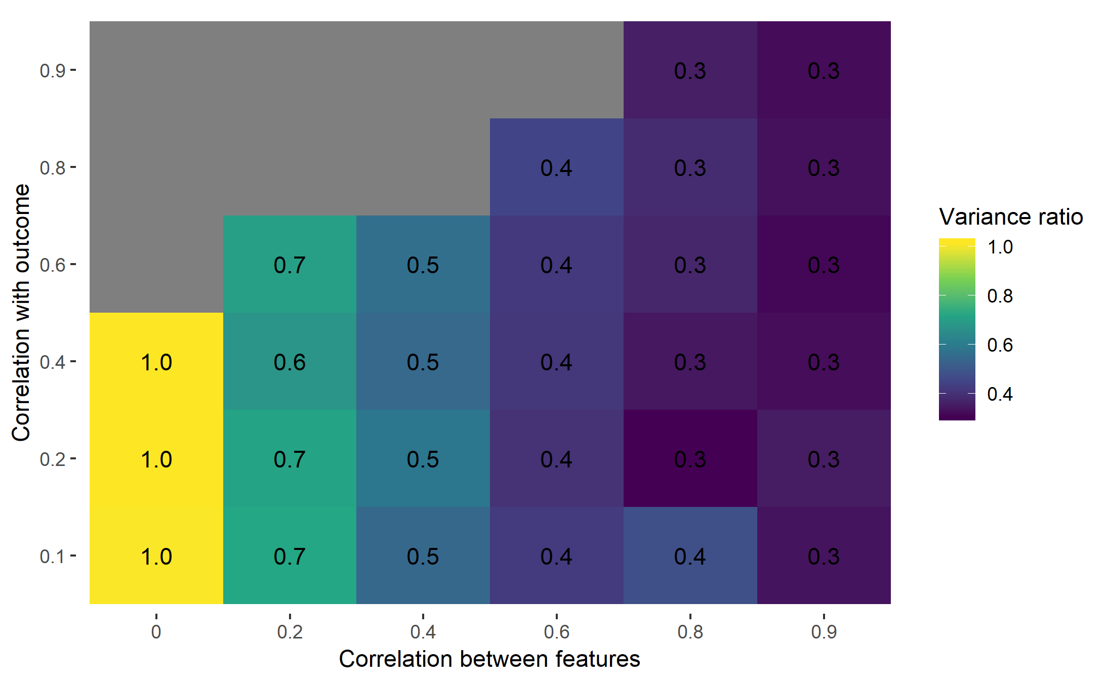
To illustrate the extent to which feature correlations affect our metric, we simulated data from a linear model with varying levels of correlation between features and calculated . The data were simulated from 3-feature multivariate standard normal distributions with uniform correlations, and (7) was calculated using the stochastic Shapley value approximations described in [3]. The results in Figure 1 suggest that even moderate levels of between-feature correlation affect the validity of variance-based measures of feature importance as approximately 50% of the model-explained variance cannot be assigned to specific features in a straightforward manner.
Recent research from [18] into kernel-based solutions to the feature correlation problem in Shapley value analysis holds promise. We do not, however, cover their approach here because it does not alter the proposed decomposition; rather, the correlation-adjusted Shapley values that they propose can be thought of as a data preprocessing step that strengthens the validity of our metric.
Applied Analysis
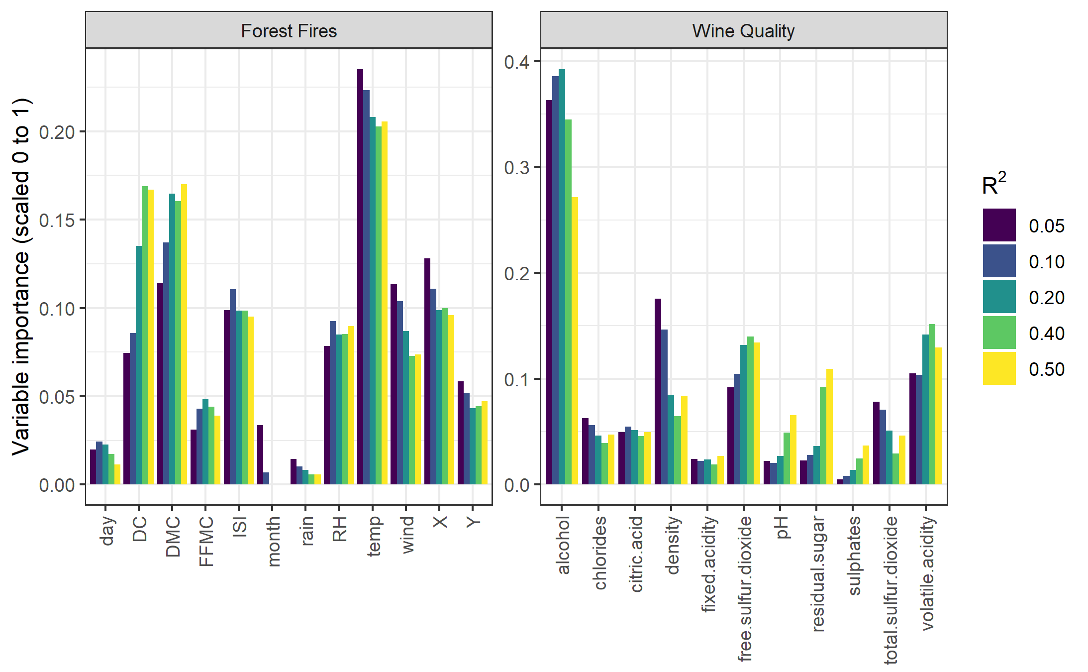
To get a sense of the stability of the proposed feature importance metric in an applied setting, we fit a series of gradient boosted decision tree models to predict (a) wine quality in the white wine dataset [19] and (b) the area burned in a forest fire in the forest fires dataset [20], both of which are available on the UCI Machine Learning Repository [21]. The models were fit with the R implementation of the catboost package [22] version 0.14.2. catboost was chosen in part because of its built-in support for the exact Shapley value calculations, titled Tree SHAP, described in [17] which are computationally inexpensive. To assess the metric’s stability, a series of five models were fit to achieve values ranging from .05 to .50 using (4). The models were fit using the default settings and increasing global values were obtained by increasing the number of iterations or trees in the ensemble from (a) ~30 to ~3,000 in the white wine dataset and (b) ~300 to ~9,000 in the forest fires dataset. The feature-level values were calculated for the training data–all available data–using our implementation of (6) available in the r2() function in the open-source R package shapFlex (https://github.com/nredell/shapFlex).
While far short of a thorough simulation, the results in Figure 2
suggest that the variance explained by each feature under the proposed
metric is potentially robust in applied analyses and likely changes
predictably across the spectrum of underfitting to overfitting.
Interestingly, the proportion of model-explained
variance that could be uniquely assigned to each feature was similar
across datasets: In the wine quality dataset, ranged
from .88 in the = .05 model to .68 in the = .50 model,
and in the forest fires dataset, ranged from .86 in
the = .05 model to .67 in the = .50 model. The
similarity of the
size of the values is likely due to the
near-identical average absolute correlation between numeric features in
each dataset–.17. The similarity in the direction of the
values–decreasing as the boosted tree models were
increasingly overfit–is more difficult to explain. One plausible
explanation is that overfitting a non-linear model to the data
increasingly captures linear and non-linear relationships in the data
that
increasingly violate the feature independence assumption in most Shapley
value and Shapley value approximation algorithms. To what extent this is
data dependent, model dependent, or Shapley value calculation dependent
remains, to our knowledge, an open research question.
Discussion
In this paper we proposed a modified version of suitable for summarizing feature importance in linear and non-linear machine learning models. This metric makes use of the additive property of Shapley values to fairly distribute the share of a model’s explained variance to each feature without the computational burden of refitting a machine learning model to various subsets of features. However, while the proposed metric has nice properties–0 to 1 scaling and a feature-level variance decomposition summing to the overall model –, the effect of overfitting and hyperparameter tuning on the stability of the decomposition needs further investigation. Additional open questions include whether this metric is best applied to model training or model testing data as well as how this metric could be extended to hierarchical or nested data structures where explaining the variability between groups or through time is of interest. Nonetheless, the proposed metric could see use by practitioners looking to better understand the models that they have built by bridging the gap between classical statistics and modern machine learning.
References
[1] Murdoch, W. J., Singh, C., Kumbier, K., Abbasi-Asl, R., & Yu, B. (2019). Interpretable machine learning: definitions, methods, and applications. arXiv preprint arXiv:1901.04592.
[2] Doshi-Velez, F., & Kim, B. (2017). Towards a rigorous science of interpretable machine learning. arXiv preprint arXiv:1702.08608.
[3] Lundberg, S. M., & Lee, S. I. (2017). A unified approach to interpreting model predictions. In Advances in Neural Information Processing Systems (pp. 4765-4774).
[4] Biecek, P. (2018). DALEX: explainers for complex predictive models in R. The Journal of Machine Learning Research, 19(1), 3245-3249.
[5] Molnar, C., Casalicchio, G., & Bischl, B. (2018). Iml: An R package for interpretable machine learning. The Journal of Open Source Software, 3(786), 10-21105.
[6] Molnar, Christoph. (2019) “Interpretable machine learning. A Guide for Making Black Box Models Explainable”. https://christophm.github.io/interpretable-ml-book/.
[7] Britton, M. (2019). VINE: Visualizing Statistical Interactions in Black Box Models. arXiv preprint arXiv:1904.00561.
[8] Grömping, U. (2015). Variable importance in regression models. Wiley Interdisciplinary Reviews: Computational Statistics, 7(2), 137-152.
[9] Wachter, S., Mittelstadt, B., & Russell, C. (2017). Counterfactual explanations without opening the black box: Automated decisions and the GDPR. Harvard Journal of Law & Technology, 31(2), 2018.
[10] Wright, S. (1921). Correlation and causation. Journal of agricultural research, 20(7), 557-585.
[11] Kvålseth, T. O. (1985). Cautionary note about R 2. The American Statistician, 39(4), 279-285.
[12] Fisher, A., Rudin, C., & Dominici, F. (2018). All Models are Wrong but many are Useful: Variable Importance for Black-Box, Proprietary, or Misspecified Prediction Models, using Model Class Reliance. arXiv preprint arXiv:1801.01489.
[13] Gelman, A., Goodrich, B., Gabry, J., & Vehtari, A. (2018). R-squared for Bayesian regression models. The American Statistician, (just-accepted), 1-6.
[14] Lideman, R., Merenda, P., & Gold, R. (1980). Introduction to bivariate and multivariate analysis scott. Scott Foresman: Glenview, IL, USA.
[15] Coleman, C. D., (2017) Decomposing the R-squared of a Regression Using the Shapley Value in SAS ®. US Census Bureau.
[16] Shapley, L. S. (1953). A value for n-person games. In Kuhn, H. W. and Tucker, A. W., editors, Contribution to the Theory of Games II (Annals of Mathematics Studies 28), pages 307–317. Princeton University Press, Princeton, NJ.
[17] Lundberg, S. M., Erion, G. G., & Lee, S. I. (2018). Consistent individualized feature attribution for tree ensembles. arXiv preprint arXiv:1802.03888.
[18] Kjersti, Aas, Jullum, Martin, & Løland, Anders (2019). Explaining individual predictions when features are dependent: More accurate approximations to Shapley values. arXiv preprint arXiv:1903.10464v2.
[19] P. Cortez, A. Cerdeira, F. Almeida, T. Matos and J. Reis. (2009). Modeling wine preferences by data mining from physicochemical properties. In Decision Support Systems, Elsevier, 47(4):547-553.
[20] P. Cortez & A. Morais. (2007). A Data Mining Approach to Predict Forest Fires using Meteorological Data. In J. Neves, M. F. Santos and J. Machado Eds., New Trends in Artificial Intelligence, Proceedings of the 13th EPIA 2007 - Portuguese Conference on Artificial Intelligence, December, Guimarães, Portugal, pp. 512-523, 2007. APPIA, ISBN-13 978-989-95618-0-9.
[21] Dua, D. & Graff, C. (2019). UCI Machine Learning Repository [http://archive.ics.uci.edu/ml]. Irvine, CA: University of California, School of Information and Computer Science.
[22] Prokhorenkova, L., Gusev, G., Vorobev, A., Dorogush, A. V., & Gulin, A. (2018). CatBoost: unbiased boosting with categorical features. In Advances in Neural Information Processing Systems (pp. 6638-6648).