City-Scale Road Extraction from Satellite Imagery v2:
Road Speeds and Travel Times

Abstract

Automated road network extraction from remote sensing imagery remains a significant challenge despite its importance in a broad array of applications. To this end, we explore road network extraction at scale with inference of semantic features of the graph, identifying speed limits and route travel times for each roadway. We call this approach City-Scale Road Extraction from Satellite Imagery v2 (CRESIv2), Including estimates for travel time permits true optimal routing (rather than just the shortest geographic distance), which is not possible with existing remote sensing imagery based methods. We evaluate our method using two sources of labels (OpenStreetMap, and those from the SpaceNet dataset), and find that models both trained and tested on SpaceNet labels outperform OpenStreetMap labels by $\geq 60\%$. We quantify the performance of our algorithm with the Average Path Length Similarity (APLS) and map topology (TOPO) graph-theoretic metrics over a diverse test area covering four cities in the SpaceNet dataset. For a traditional edge weight of geometric distance, we find an aggregate of 5% improvement over existing methods for SpaceNet data. We also test our algorithm on Google satellite imagery with OpenStreetMap labels, and find a 23% improvement over previous work. Metric scores decrease by only 4% on large graphs when using travel time rather than geometric distance for edge weights, indicating that optimizing routing for travel time is feasible with this approach.

1 Introduction

The automated extraction of roads applies to a multitude of long-term efforts: improving access to health services, urban planning, and improving social and economic welfare. This is particularly true in developing countries that have limited resources for manually intensive labeling and are under-represented in current mapping. Updated maps are also crucial for such time sensitive efforts as determining communities in greatest need of aid, effective positioning of logistics hubs, evacuation planning, and rapid response to acute crises.

Existing data collection methods such as manual road labeling or aggregation of mobile GPS tracks are currently insufficient to properly capture either underserved regions (due to infrequent data collection), or the dynamic changes inherent to road networks in rapidly changing environments. For example, in many regions of the world OpenStreetMap (OSM) [23] road networks are remarkably complete. Yet, in developing nations OSM labels are often missing metadata tags (such as speed limit or number of lanes), or are poorly registered with overhead imagery (i.e., labels are offset from the coordinate system of the imagery), see Figure 1. An active community works hard to keep the road network up to date, but such tasks can be challenging and time consuming in the face of large scale disasters. For example, following Hurricane Maria, it took the Humanitarian OpenStreetMap Team (HOT) over two months to fully map Puerto Rico [21]. Furthermore, in large-scale disaster response scenarios, pre-existing datasets such as population density and even geographic topology may no longer be accurate, preventing responders from leveraging this data to jump start mapping efforts.

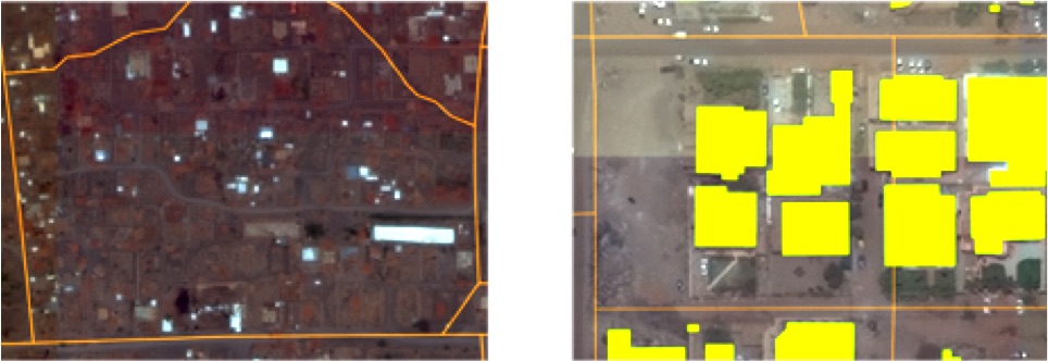
Figure 1: Potential issues with OSM data. Left: OSM roads (orange) overlaid on Khartoum imagery; the east-west road in the center is erroneously unlabeled. Right: OSM roads (orange) and SpaceNet buildings (yellow); in some cases road labels are misaligned and intersect buildings.

The frequent revisits of satellite imaging constellations may accelerate existing efforts to quickly update road network and routing information. Of particular utility is estimating the time it takes to travel various routes in order to minimize response times in various scenarios; unfortunately existing algorithms based upon remote sensing imagery cannot provide such estimates. A fully automated approach to road network extraction and travel time estimation from satellite imagery therefore warrants investigation, and is explored in the following sections. In Section 2 we discuss related work, while Section 3 details our graph extraction algorithm that infers a road network with semantic features directly from imagery. In Section 4 we discuss the datasets used and our method for assigning road speed estimates based on road geometry and metadata tags. Section 5 discusses the need for modified metrics to measure our semantic graph, and Section 6 covers our experiments to extract road networks from multiple datasets. Finally in Sections 7 and 8 we discuss our findings and conclusions.

2 Related Work

Extracting road pixels in small image chips from aerial imagery has a rich history (e.g. [34], [20] [30], [34], [26], [16]). These algorithms typically use a segmentation + post-processing approach combined with lower resolution imagery (resolution $\geq 1$ meter), and OpenStreetMap labels. Some more recent efforts (e.g. [35]) have utilized higher resolution imagery (0.5 meter) with pixel-based labels [9].

Extracting road networks directly has also garnered increasing academic interest as of late. [27] attempted road extraction via a Gibbs point process, while [32] showed some success with road network extraction with a conditional random field model. [6] used junction-point processes to recover line networks in both roads and retinal images, while [28] extracted road networks by representing image data as a graph of potential paths. [19] extracted road centerlines and widths via OSM and a Markov random field process, and [17] used a topology-aware loss function to extract road networks from aerial features as well as cell membranes in microscopy.

Of greatest interest for this work are a trio of recent papers that improved upon previous techniques. DeepRoadMapper [18] used segmentation followed by $A^{*}$ search, applied to the not-yet-released TorontoCity Dataset. The RoadTracer paper [3] utilized an interesting approach that used OSM labels to directly extract road networks from imagery without intermediate steps such as segmentation. While this approach is compelling, according to the authors it “struggled in areas where roads were close together” [2] and underperforms other techniques such as segmentation + post-processing when applied to higher resolution data with dense labels. [4] used a connectivity task termed Orientation Learning combined with a stacked convolutional module and a SoftIOU loss function to effectively utilize the mutual information between orientation learning and segmentation tasks to extract road networks from satellite imagery, noting improved performance over [3]. Given that [3] noted superior performance to [18] (as well as previous methods), and [4] claimed improved performance over both [3] and [18], we compare our results to RoadTracer [3] and Orientation Learning [4].

We build upon CRESI v1 [10] that scaled up narrow-field road network extraction methods. In this work we focus primarily on developing methodologies to infer road speeds and travel times, but also improve the segmentation, gap mitigation, and graph curation steps of [10], as well as improve inference speed.

3 Road Network Extraction Algorithm

Our approach is to combine novel segmentation approaches, improved post-processing techniques for road vector simplification, and road speed extraction using both vector and raster data. Our greatest contribution is the inference of road speed and travel time for each road vector, a task that has not been attempted in any of the related works described in Section 2. We utilize satellite imagery and geo-coded road centerline labels (see Section 4 for details on datasets) to build training datasets for our models.

We create training masks from road centerline labels assuming a mask halfwidth of 2 meters for each edge. While scaling the training mask width with the full width of the road is an option (e.g. a four lane road will have a greater width than a two lane road), since the end goal is road centerline vector extraction, we utilize the same training mask width for all roadways. Too wide of a road buffer inhibits the ability to identify the exact centerline of the road, while too thin of a buffer reduces the robustness of the model to noise and variance in label quality; we find that a 2 meter buffer provides the best tradeoff between these two extremes.

We have two goals: extract the road network over large areas, and assess travel time along each roadway. In order to assess travel time we assign a speed limit to each roadway based on metadata tags such as road type, number of lanes, and surface construction.

We assign a maximum safe traversal speed of 10 - 65 mph to each segment based on the road metadata tags. For example, a paved one-lane residential road has a speed limit of 25 mph, a three-lane paved motorway can be traversed at 65 mph, while a one-lane dirt cart track has a traversal speed of 15 mph. See Appendix A for further details. This approach is tailored to disaster response scenarios, where safe navigation speeds likely supersede government-defined speed limits. We therefore prefer estimates based on road metadata over government-defined speed limits, which may be unavailable or inconsistent in many areas.

3.1 Multi-Class Segmentation

We create multi-channel training masks by binning the road labels into a 7-layer stack, with channel 0 detailing speeds between 1-10 mph, channel 1 between 11-20 mph, etc. (see Figure 2). We train a segmentation model inspired by the winning SpaceNet 3 algorithm [1], and use a ResNet34 [12] encoder with a U-Net [24] inspired decoder. We include skip connections every layer of the network, and use an Adam optimizer. We explore various loss functions, including binary cross entropy, Dice, and focal loss [14], and find the best performance with $\alpha_{mc}=0.75$ and a custom loss function of:

$$\mathcal{L}=\alpha_{mc}\mathcal{L}_{\text{focal}}+(1-\alpha_{mc})\mathcal{L}_{\text{dice}}$$ (1)

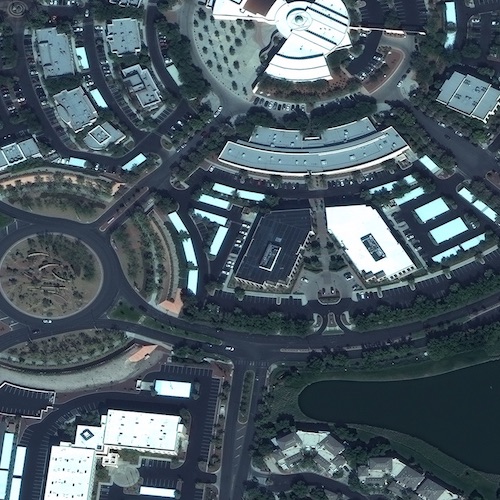
(a) Input Image

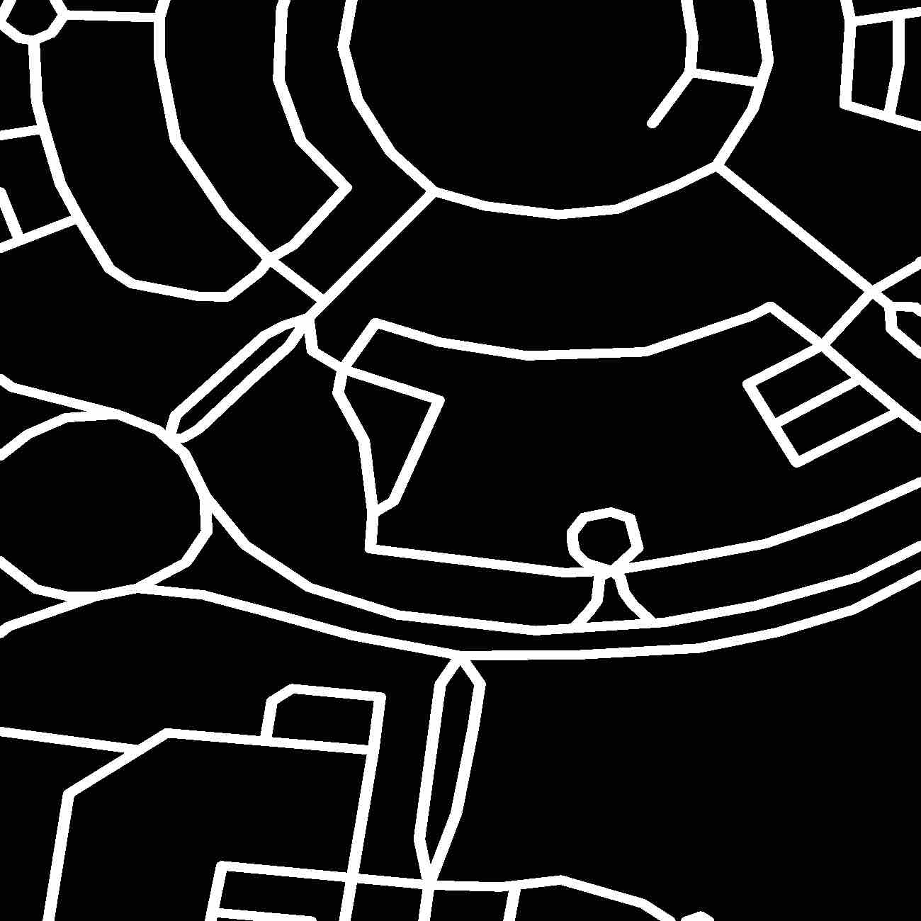
(b) Binary Training Mask

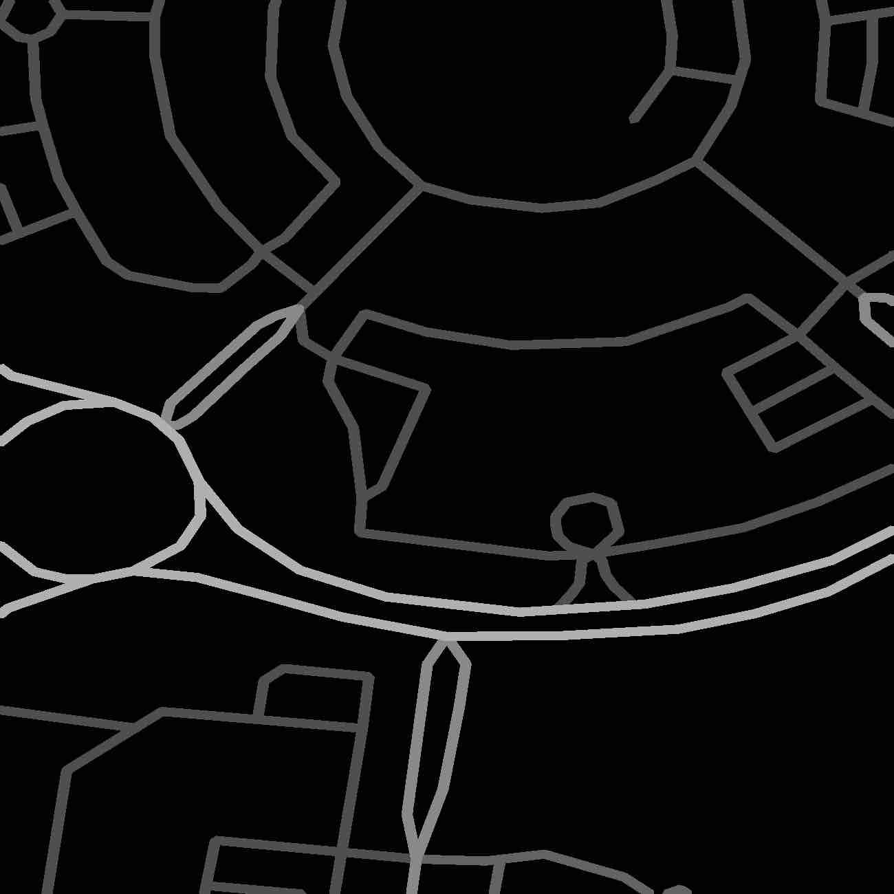
(c) Continuous Training Mask

(d) Multi-class Training Mask

Figure 2: Training data. (a) Input image. (b) Typical binary road training mask (not used in this study). (c) Continuous training mask, whiter denotes higher speeds. (d) Multi-class mask showing individual speed channels: red = 21-30 mph, green = 31-40 mph, blue = 41-50 mph.

3.2 Continuous Mask Segmentation

A second segmentation method renders continuous training masks from the road speed labels. Rather than the typical binary mask, we linearly scale the mask pixel value with speed limit, assuming a maximum speed of 65 mph (see Figure 2).

We use a similar network architecture to the previous section (ResNet34 encoder with a U-Net inspired decoder), though we use a loss function that utilizes cross entropy (CE) rather than focal loss ($\alpha_{c}=0.75$):

$$\mathcal{L}=\alpha_{c}\mathcal{L}_{\text{CE}}+(1-\alpha_{c})\mathcal{L}_{\text{dice}}$$ (2)

3.3 Graph Extraction Procedure

The output of the segmentation mask step detailed above is subsequently refined into road vectors. We begin by smoothing the output mask with a Gaussian kernel of 2 meters. This mask is then refined using opening and closing techniques with a similar kernel size of 2 meters, as well as removing small object artifacts or holes with an area less than 30 square meters. From this refined mask we create a skeleton (e.g.  sckit-image skeletonize [25]). This skeleton is rendered into a graph structure with a version of the sknw package [33] package modified to work on very large images. This process is detailed in Figure 3. The graph created by this process contains length information for each edge, but no other metadata. To close small gaps and remove spurious connections not already corrected by the mask refinement procedures, we remove disconnected subgraphs with an integrated path length of less than a certain length (6 meters for small image chips, and 80 meters for city-scale images). We also follow [1] and remove terminal vertices that lie on an edge less than 3 meters in length, and connect terminal vertices if the distance to the nearest non-connected node is less than 6 meters.

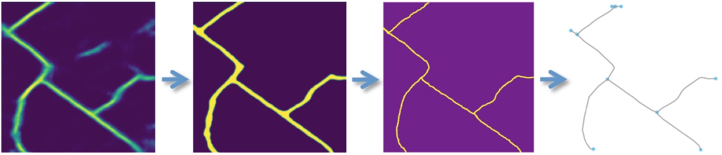
Figure 3: Graph extraction procedure. Left: raw mask output. Left center: refined mask. Right center: mask skeleton. Right: graph structure.

3.4 Speed Estimation Procedure

We estimate travel time for a given road edge by leveraging the speed information encapsulated in the prediction mask. The majority of edges in the graph are composed of multiple segments; accordingly, we attempt to estimate the speed of each segment in order to determine the mean speed of the edge. This is accomplished by analyzing the prediction mask at the location of the segment midpoints. For each segment in the edge, at the location of the midpoint of the segment we extract a small $8\times 8$ pixel patch from the prediction mask. The speed of the patch is estimated by filtering out low probability values (likely background), and averaging the remaining pixels (see Figure 4). In the multi-class case, if the majority of the the high confidence pixels in the prediction mask patch belong to channel 3 (corresponding to 31-40 mph), we would assign the speed at that patch to be 35 mph. For the continuous case the inferred speed is simply directly proportional to the mean pixel value.

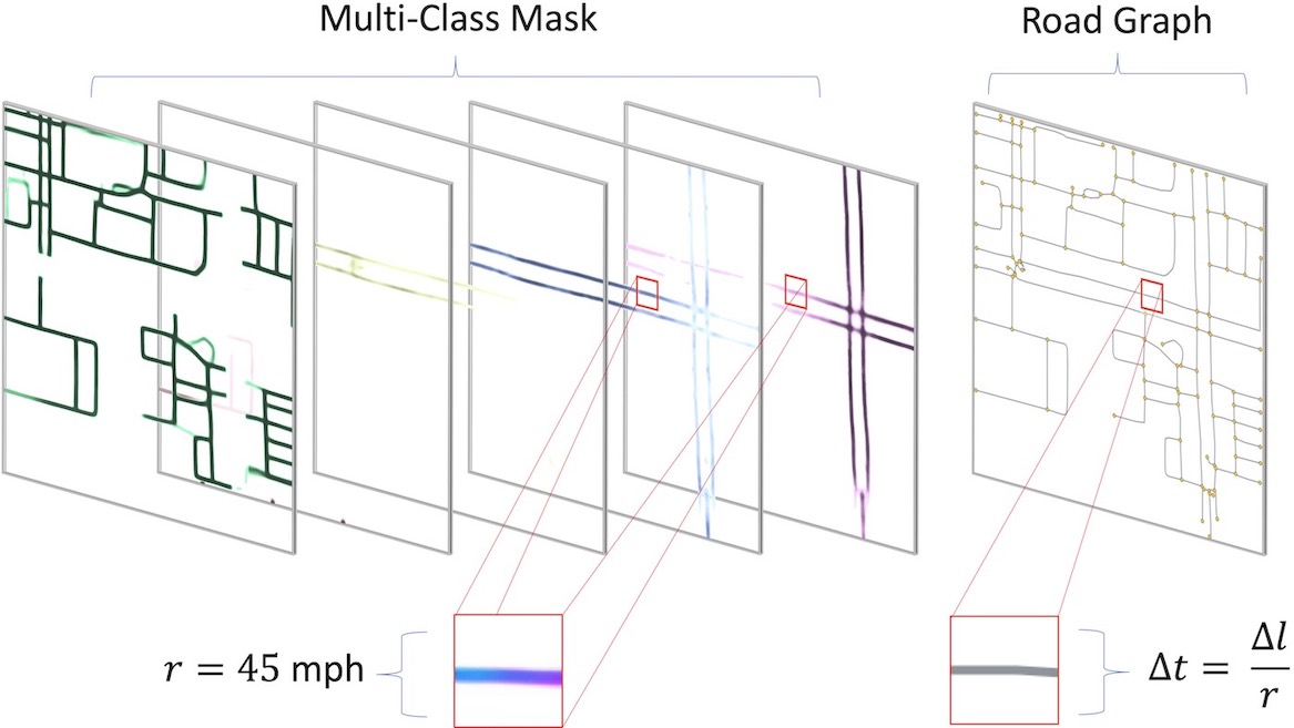
Figure 4: Speed estimation procedure. Left: Sample multi-class prediction mask; the speed ($r$) of an individual patch (red square) can be inferred by measuring the signal from each channel. Right: Computed road graph; travel time ($\Delta t$) is given by speed ($r$) and segment length ($\Delta l$).

The travel time for each edge is in theory the path integral of the speed estimates at each location along the edge. But given that each roadway edge is presumed to have a constant speed limit, we refrain from computing the path integral along the graph edge. Instead, we estimate the speed limit of the entire edge by taking the mean of the speeds at each segment midpoint. Travel time is then calculated as edge length divided by mean speed.

3.5 Scaling to Large Images

The process detailed above works well for small input images, yet fails for large images due to a saturation of GPU memory. For example, even for a relatively simple architecture such as U-Net [24], typical GPU hardware (NVIDIA Titan X GPU with 12 GB memory) will saturate for images greater than $\sim 2000\times 2000$ pixels in extent and reasonable batch sizes $>4$. In this section we describe a straightforward methodology for scaling up the algorithm to larger images. We call this approach City-Scale Road Extraction from Satellite Imagery v2 (CRESIv2). The essence of this approach is to combine the approach of Sections 3.1 - 3.4 with the Broad Area Satellite Imagery Semantic Segmentation (BASISS) [7] methodology. BASISS returns a road pixel mask for an arbitrarily large test image (see Figure 5), which we then leverage into an arbitrarily large graph.

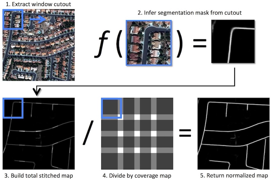
Figure 5: Large image segmentation. BASISS process of segmenting an arbitarily large satellite image [7].

The final algorithm is given by Table 1. The output of the CRESIv2 algorithm is a NetworkX [11] graph structure, with full access to the many algorithms included in this package.

Table 1: CRESIv2 Inference Algorithm

Step	Description
1	Split large test image into smaller windows
2	Apply multi-class segmentation model to each window
$\,\,2_{\rm b}$	*  Apply remaining (3) cross-validation models
$\,\,2_{\rm c}$	*  For each window, merge the 4 predictions
3	Stitch together the total normalized road mask
4	Clean road mask with opening, closing, smoothing
5	Skeletonize flattened road mask
6	Extract graph from skeleton
7	Remove spurious edges and close small gaps in graph
8	Estimate local speed limit at midpoint of each segment
9	Assign travel time to each edge from aggregate speed
	* Optional

4 Datasets

Many existing publicly available labeled overhead or satellite imagery datasets tend to be relatively small, or labeled with lower fidelity than desired for foundational mapping. For example, the International Society for Photogrammetry and Remote Sensing (ISPRS) semantic labeling benchmark [13] dataset contains high quality 2D semantic labels over two cities in Germany; imagery is obtained via an aerial platform and is 3 or 4 channel and 5-10 cm in resolution, though covers only 4.8 km². The TorontoCity Dataset [31] contains high resolution 5-10 cm aerial 4-channel imagery, and $\sim 700$ km² of coverage; building and roads are labeled at high fidelity (among other items), but the data has yet to be publicly released. The Massachusetts Roads Dataset [15] contains 3-channel imagery at 1 meter resolution, and $2600$ km² of coverage; the imagery and labels are publicly available, though labels are scraped from OpenStreetMap and not independently collected or validated. The large dataset size, higher 0.3 m resolution, and hand-labeled and quality controlled labels of SpaceNet [29] provide an opportunity for algorithm improvement. In addition to road centerlines, the SpaceNet dataset contains metadata tags for each roadway including: number of lanes, road type (e.g.  motorway, residential, etc), road surface type (paved, unpaved), and bridgeway (true/false).

4.1 SpaceNet Data

Our primary dataset accordingly consists of the SpaceNet 3 WorldView-3 DigitalGlobe satellite imagery (30 cm/pixel) and attendant road centerline labels. Imagery covers 3000 square kilometers, and over 8000 km of roads are labeled [29]. Training images and labels are tiled into $1300\times 1300$ pixel ($\approx 160,000\,\rm{m^{2}}$) chips (see Figure 6).

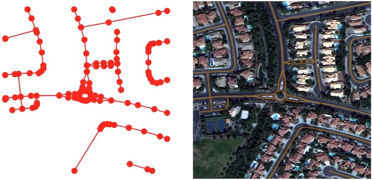
Figure 6: SpaceNet training chip. Left: SpaceNet GeoJSON road label. Right: $400\times 400$ meter image overlaid with road centerline labels (orange).

To test the city-scale nature of our algorithm, we extract large test images from all four of the SpaceNet cities with road labels: Las Vegas, Khartoum, Paris, and Shanghai. As the labeled SpaceNet test regions are non-contiguous and irregularly shaped, we define rectangular subregions of the images where labels do exist within the entirety of the region. These test regions total 608 km², with a total road length of 9065 km. See Appendix B for further details.

4.2 Google / OSM Dataset

We also evaluate performance with the satellite imagery corpus used by [3]. This dataset consists of Google satellite imagery at 60 cm/pixel over 40 cities, 25 for training and 15 for testing. Vector labels are scraped from OSM, and we use these labels to build training masks according the procedures described above. Due to the high variability in OSM road metadata density and quality, we refrain from inferring road speed from this dataset, and instead leave this for future work.

5 Evaluation Metrics

Historically, pixel-based metrics (such as IOU or F1 score) have been used to assess the quality of road proposals, though such metrics are suboptimal for a number of reasons (see [29] for further discussion). Accordingly, we use the graph-theoretic Average Path Length Similarity (APLS) and map topology (TOPO) [5] metrics designed to measure the similarity between ground truth and proposal graphs.

5.1 APLS Metric

To measure the difference between ground truth and proposal graphs, the APLS [29] metric sums the differences in optimal path lengths between nodes in the ground truth graph G and the proposal graph G’, with missing paths in the graph assigned a score of 0. The APLS metric scales from 0 (poor) to 1 (perfect). Missing nodes of high centrality will be penalized much more heavily by the APLS metric than missing nodes of low centrality. The definition of shortest path can be user defined; the natural first step is to consider geographic distance as the measure of path length (APLS_length), but any edge weights can be selected. Therefore, if we assign a travel time estimate to each graph edge we can use the APLS_time metric to measure differences in travel times between ground truth and proposal graphs.

For large area testing, evaluation takes place with the APLS metric adapted for large images: no midpoints along edges and a maximum of 500 random control nodes.

5.2 TOPO Metric

The TOPO metric [5] is an alternative metric for computing road graph similarity. TOPO compares the nodes that can be reached within a small local vicinity of a number of seed nodes, categorizing proposal nodes as true positives, false positives, or false negatives depending on whether they fall within a buffer region (referred to as the “hole size”). By design, this metric evaluates local subgraphs in a small subregion ($\sim 300$ meters in extent), and relies upon physical geometry. Connections between greatly disparate points ($>300$ meters apart) are not measured, and the reliance upon physical geometry means that travel time estimates cannot be compared.

6 Experiments

We train CRESIv2 models on both the SpaceNet and Google/OSM datasets. For the SpaceNet models, we use the 2780 images/labels in the SpaceNet 3 training dataset. The Google/OSM models are trained with the 25 training cities in [3]. All segmentation models use a road centerline halfwidth of 2 meters, and withhold 25% of the training data for validation purposes. Training occurs for 30 epochs. Optionally, one can create an ensemble of 4 folds (i.e. the 4 possible unique combinations of 75% train and 25% validate) to train 4 different models. This approach may increase model robustness, at the cost of increased compute time. As inference speed is a priority, all results shown below use a single model, rather than the ensemble approach.

For the Google / OSM data, we train a segmentation model as in Section 3.1, though with only a single class since we forego speed estimates with this dataset.

6.1 SpaceNet Test Corpus Results

We compute both APLS and TOPO performance for the $400\times 400$ meter image chips in the SpaceNet test corpus, utilizing an APLS buffer and TOPO hole size of 4 meters (implying proposal road centerlines must be within 4 meters of ground truth), see Table 2. An example result is shown in Figure 7. Reported errors ($\pm 1\sigma$) reflect the relatively high variance of performance among the various test scenes in the four SpaceNet cities. Table 2 indicates that the continuous mask model struggles to accurately reproduce road speeds, due in part to the model’s propensity to predict high pixel values for for high confidence regions, thereby skewing speed estimates. In the remainder of the paper, we only consider the multi-class model. Table 2 also demonstrates that for the multi-class model the APLS score is still 0.58 when using travel time as the weight, which is only $13\%$ lower than when weighting with geometric distance.

Table 2: Performance on SpaceNet Test Chips

Model	TOPO	APLSlength	APLStime
Multi-Class	$0.53\pm 0.23$	$0.68\pm 0.21$	$0.58\pm 0.21$
Continuous	$0.52\pm 0.25$	$0.68\pm 0.22$	$0.39\pm 0.18$

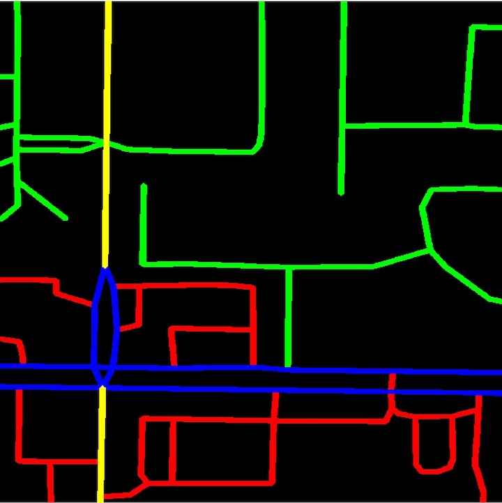
(a) Ground truth mask

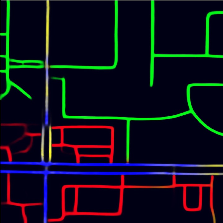
(b) Predicted mask

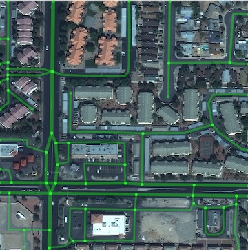
(c) Ground truth network

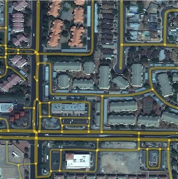
(d) Predicted network

Figure 7: Algorithm performance on SpaceNet. (a) Ground truth and (b) predicted multi-class masks: red = 21-30 mph, green = 31-40 mph, blue = 41-50 mph, yellow = 51-60 mph. (c) Ground truth and (d) predicted graphs overlaid on the SpaceNet test chip; edge widths are proportional to speed limit. The scores for this proposal are APLS${}_{\rm{length}}=0.80$ and APLS${}_{\rm{time}}=0.64$.

6.2 Comparison of SpaceNet to OSM

As a means of comparison between OSM and SpaceNet labels, we use our algorithm to train two models on SpaceNet imagery. One model uses ground truth segmentation masks rendered from OSM labels, while the other model uses ground truth masks rendered from SpaceNet labels. Table 3 displays APLS scores computed over a subset of the SpaceNet test chips, and demonstrates that the model trained and tested on SpaceNet labels is far superior to other combinations, with a $\approx 60-100\%$ improvement in APLS_length score. This is likely due in part to the the more uniform labeling schema and validation procedures adopted by the SpaceNet labeling team, as well as the superior registration of labels to imagery in SpaceNet data. The poor performance of the SpaceNet-trained OSM-tested model is likely due to a combination of: different labeling density between the two datasets, and differing projections of labels onto imagery for SpaceNet and OSM data. Figure 8 and Appendix C illustrate the difference between predictions returned by the OSM and SpaceNet models.

Table 3: OSM and SpaceNet Performance

Training Labels	Test Labels	APLSlength
OSM	OSM	0.47
OSM	SpaceNet	0.46
SpaceNet	OSM	0.39
SpaceNet	SpaceNet	0.77

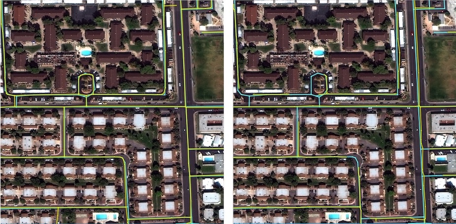
Figure 8: SpaceNet compared to OSM. Road predictions (yellow) and ground truth SpaceNet labels (blue) for a Las Vegas image chip. SpaceNet model predictions (left) score APLS${}_{\rm{length}}=0.94$, while OSM model predictions (right) struggle in this scene with significant offset and missing roads, yielding APLS${}_{\rm{length}}=0.29$.

6.3 Ablation Study

In order to assess the relative importance of various improvements to our baseline algorithm, we perform ablation studies on the final algorithm. For evaluation purposes we utilize the the same subset of test chips as in Section 6.2, and the APLS_length metric. Table 4 demonstrates that advanced post-processing significantly improves scores. Using a more complex architecture also improves the final prediction. Applying four folds improves scores very slightly, though at the cost of significantly increased algorithm runtime. Given the minimal improvement afforded by the ensemble step, all reported results use only a single model.

Table 4: Road Network Ablation Study

	Description	APLS
1	Extract graph directly from simple U-Net model	0.56
2	Apply opening, closing, smoothing processes	0.66
3	Close larger gaps using edge direction and length	0.72
4	Use ResNet34 + U-Net architecture	0.77
5	Use 4 fold ensemble	0.78

6.4 Large Area SpaceNet Results

We apply the CRESIv2 algorithm described in Table 1 to the large area SpaceNet test set covering 608 km². Evaluation takes place with the APLS metric adapted for large images (no midpoints along edges and a maximum of 500 random control nodes), along with the TOPO metric, using a buffer size (for APLS) or hole size (for TOPO) of 4 meters. We report scores in Table 5 as the mean and standard deviation of the test regions of in each city. Table 5 reveals an overall $\approx 4\%$ decrease in APLS score when using speed versus length as edge weights. This is somewhat less than the decrease of 13% noted in Table 2, due primarily to the fewer edge effects from larger testing regions. Table 5 indicates a large variance in scores across cities; locales like Las Vegas with wide paved roads and sidewalks to frame the roads are much easier than Khartoum, which has a multitude of narrow, dirt roads and little differentiation in color between roadway and background. Figure 9 and Appendix D display the graph output for various urban environments.

Table 5: SpaceNet Large Area Performance

Test Region	TOPO	APLSlength	APLStime
Khartoum	$0.53\pm 0.09$	$0.64\pm 0.10$	$0.61\pm 0.05$
Las Vegas	$0.63\pm 0.02$	$0.81\pm 0.04$	$0.79\pm 0.02$
Paris	$0.43\pm 0.01$	$0.66\pm 0.04$	$0.65\pm 0.02$
Shanghai	$0.45\pm 0.03$	$0.55\pm 0.13$	$0.51\pm 0.11$
Total	$0.51\pm 0.02$	$0.67\pm 0.04$	$0.64\pm 0.03$

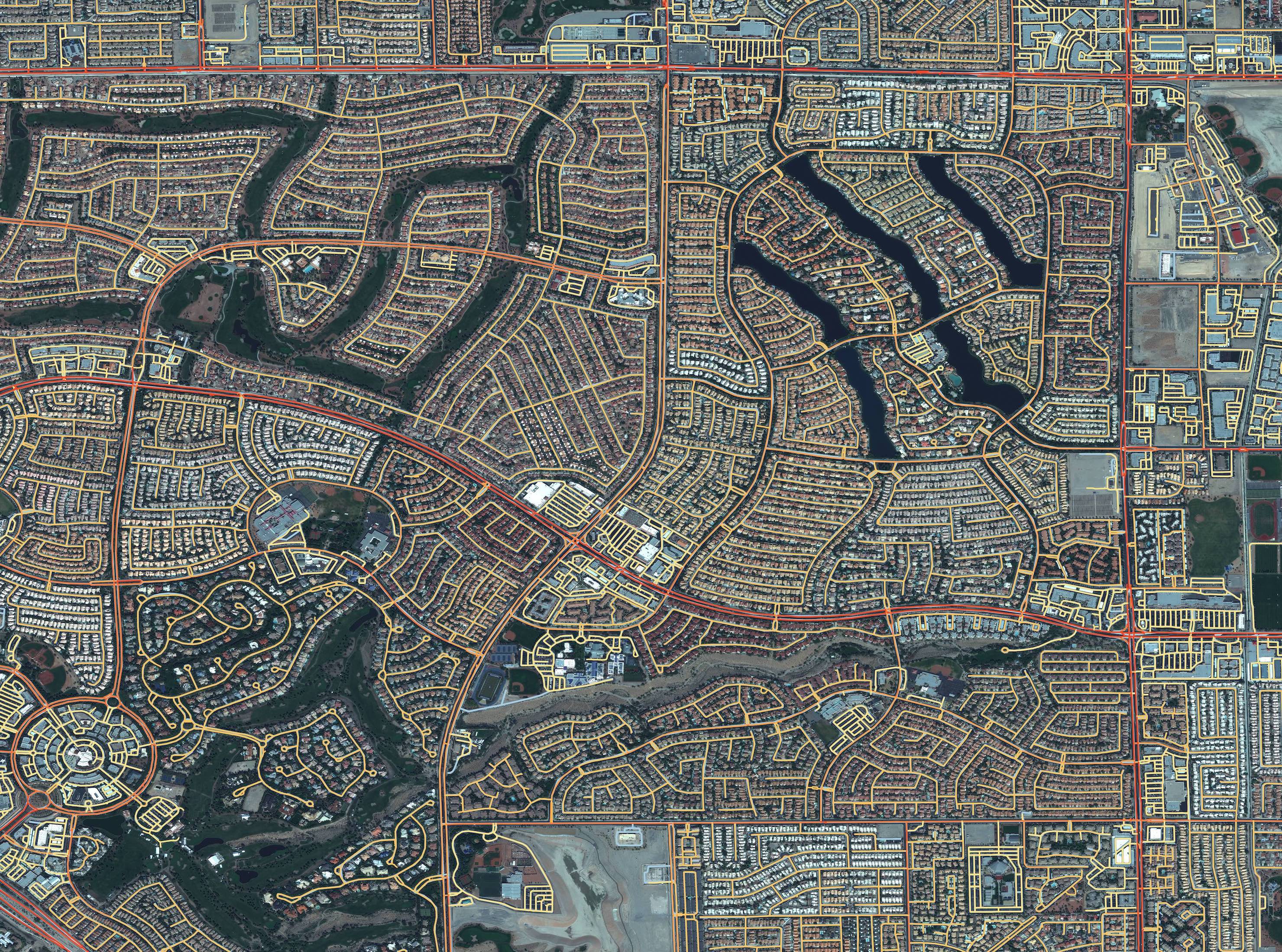
(a)

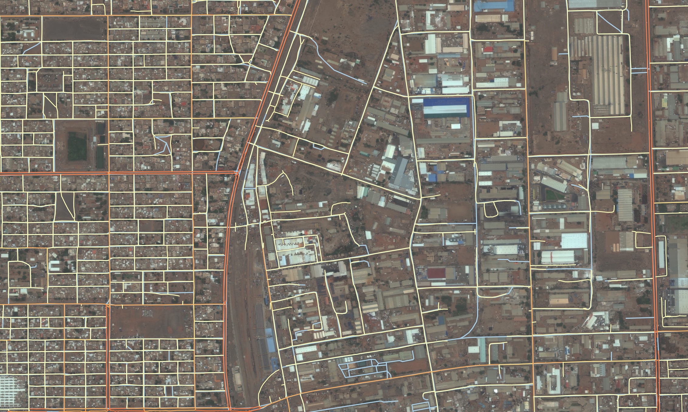
(b)

Figure 9: CRESIv2 road speed. Output of CRESIv2 inference as applied to the SpaceNet large area test dataset. Predicted roads are colored by inferred speed limit, from yellow (20 mph) to red (65 mph). Ground truth labels are shown in gray. Top: Las Vegas: APLS${}_{\rm{length}}=0.85$ and APLS${}_{\rm{time}}=0.82$. Bottom: A smaller region of Khartoum: APLS${}_{\rm{length}}=0.71$ and the APLS${}_{\rm{time}}=0.67$.

6.5 Google / OSM Results

Applying our methodology to 60 cm Google imagery with OSM labels achieves state of the art results. For the same 4 m APLS buffer used above, we achieve a score of APLS${}_{\rm{length}}=0.53\pm 0.11$. This score is consistent with the results of Table 3, and compares favorably to previous methods (see Table 6 and Figure 10).

6.6 Comparison to Previous Work

Table 6 demonstrates that CRESIv2 improves upon existing methods for road extraction, both on the $400\times 400$ m SpaceNet image chips at 30 cm resolution, as well as 60 cm Google satellite imagery with OSM labels. To allow a direct comparison in Table 6, we report TOPO scores with the 15 m hole size used in [3]. A qualitative comparison is shown in Figure 10 and Appendices E and F, illustrating that our method is more complete and misses fewer small roadways and intersections than previous methods.

Table 6: Performance Comparison

Algorithm	Google / OSM	SpaceNet
	(TOPO)	(APLSlength)
DeepRoadMapper [18]	0.37	0.51
RoadTracer [3]	0.43	0.58
OrientationLearning [4]	-	0.64
CRESIv2 (Ours)	0.53	0.67

• ¹ from Table 4 of [4]

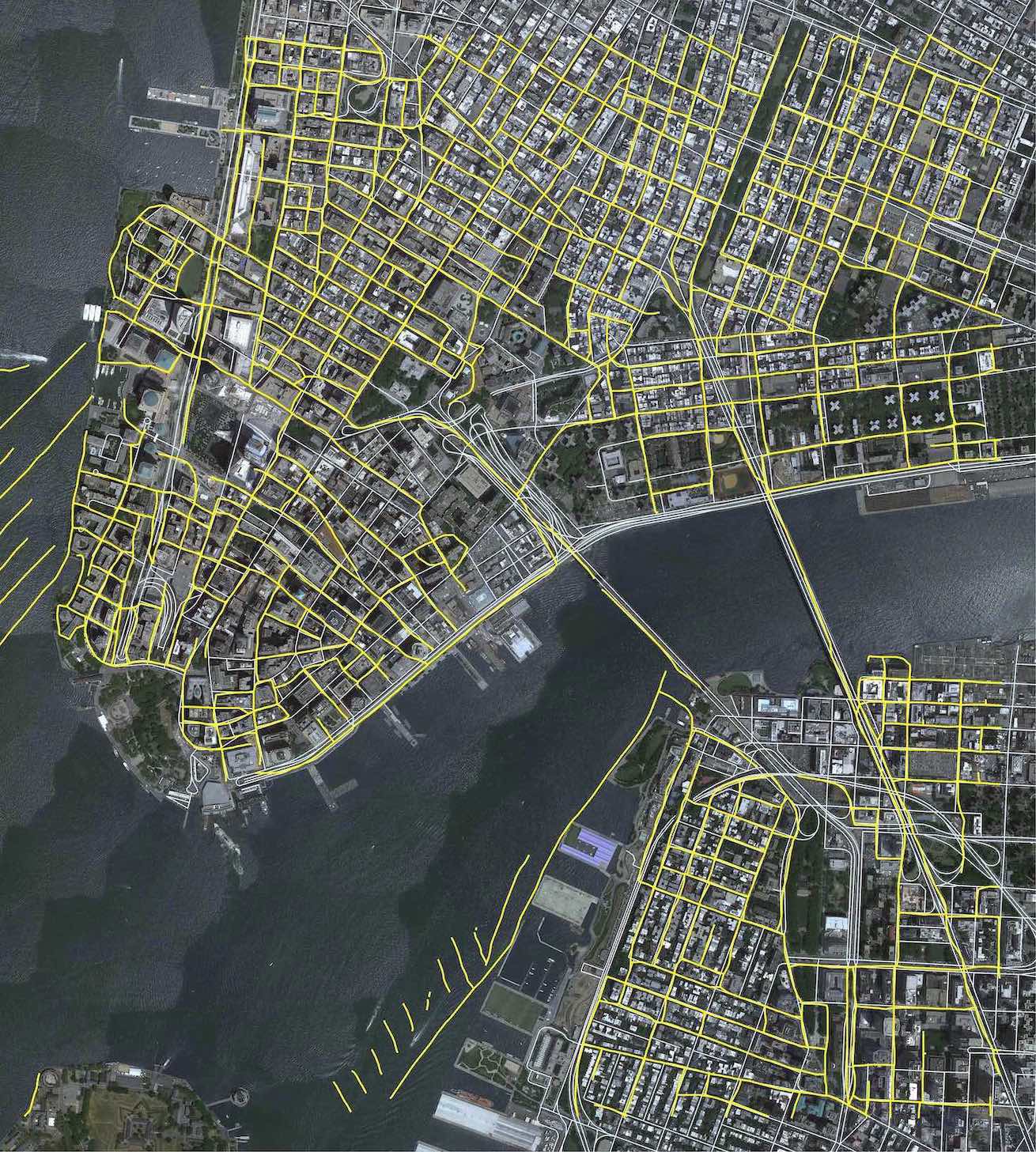
(a)

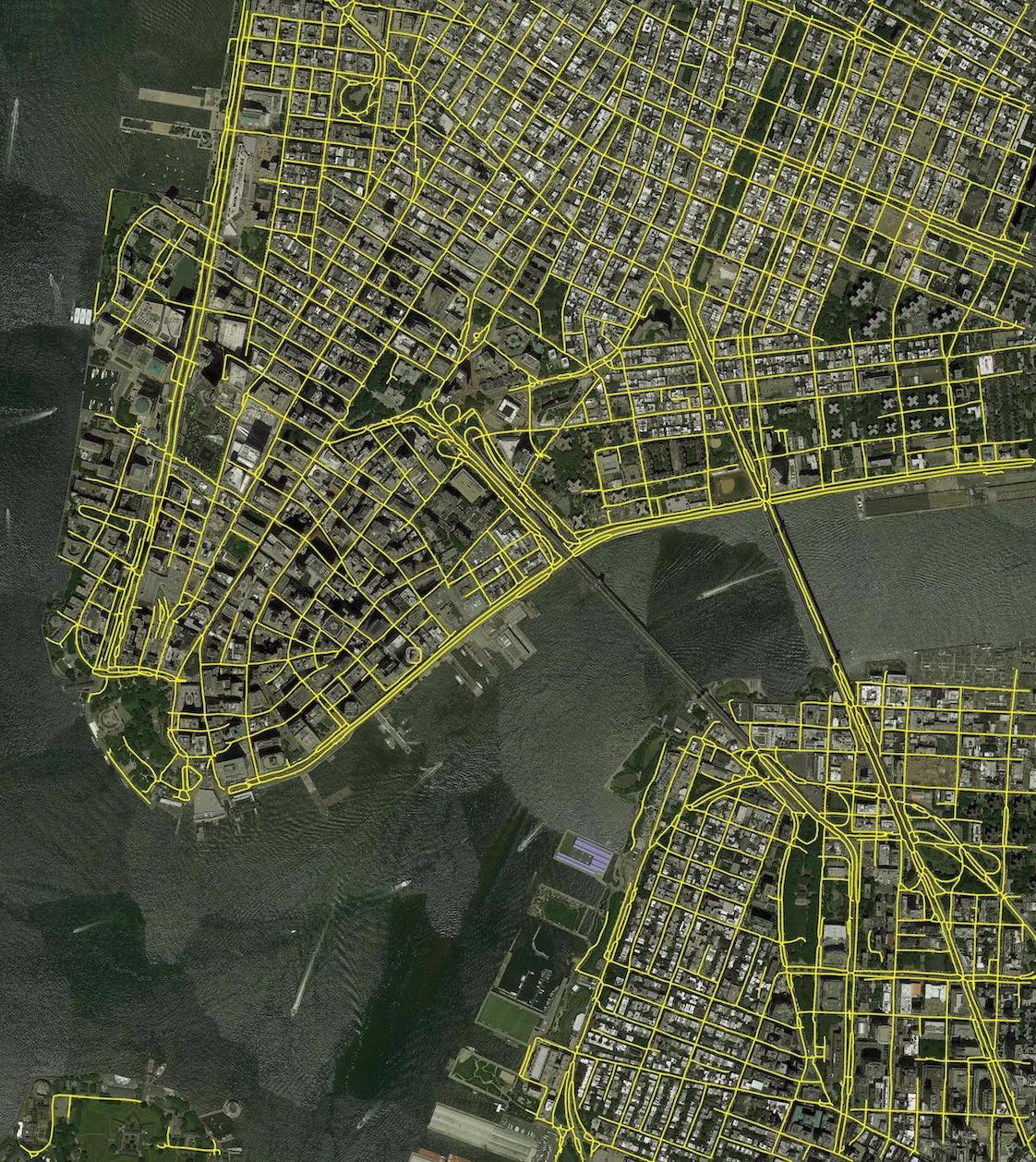
(b)

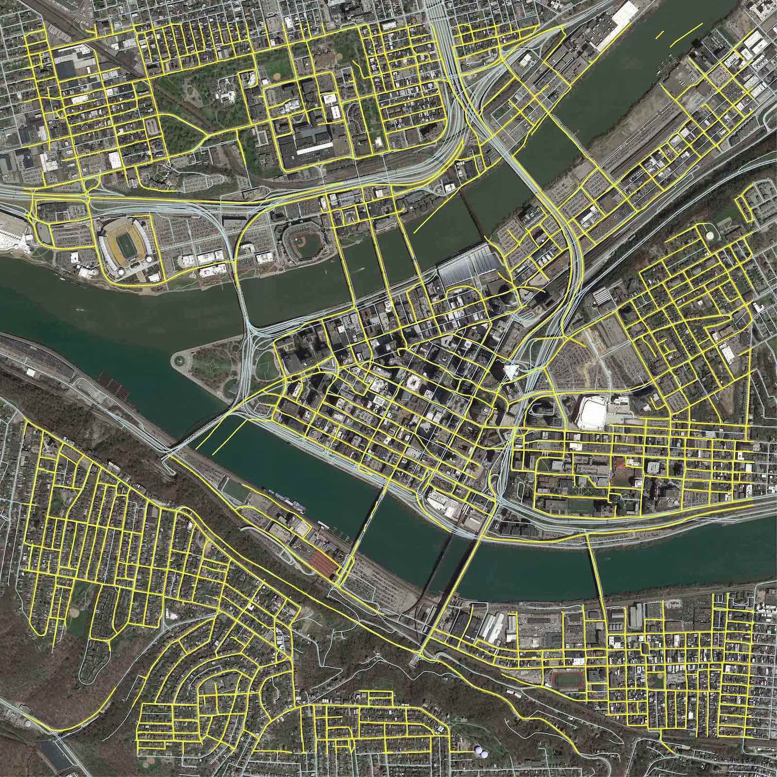
(c) RoadTracer

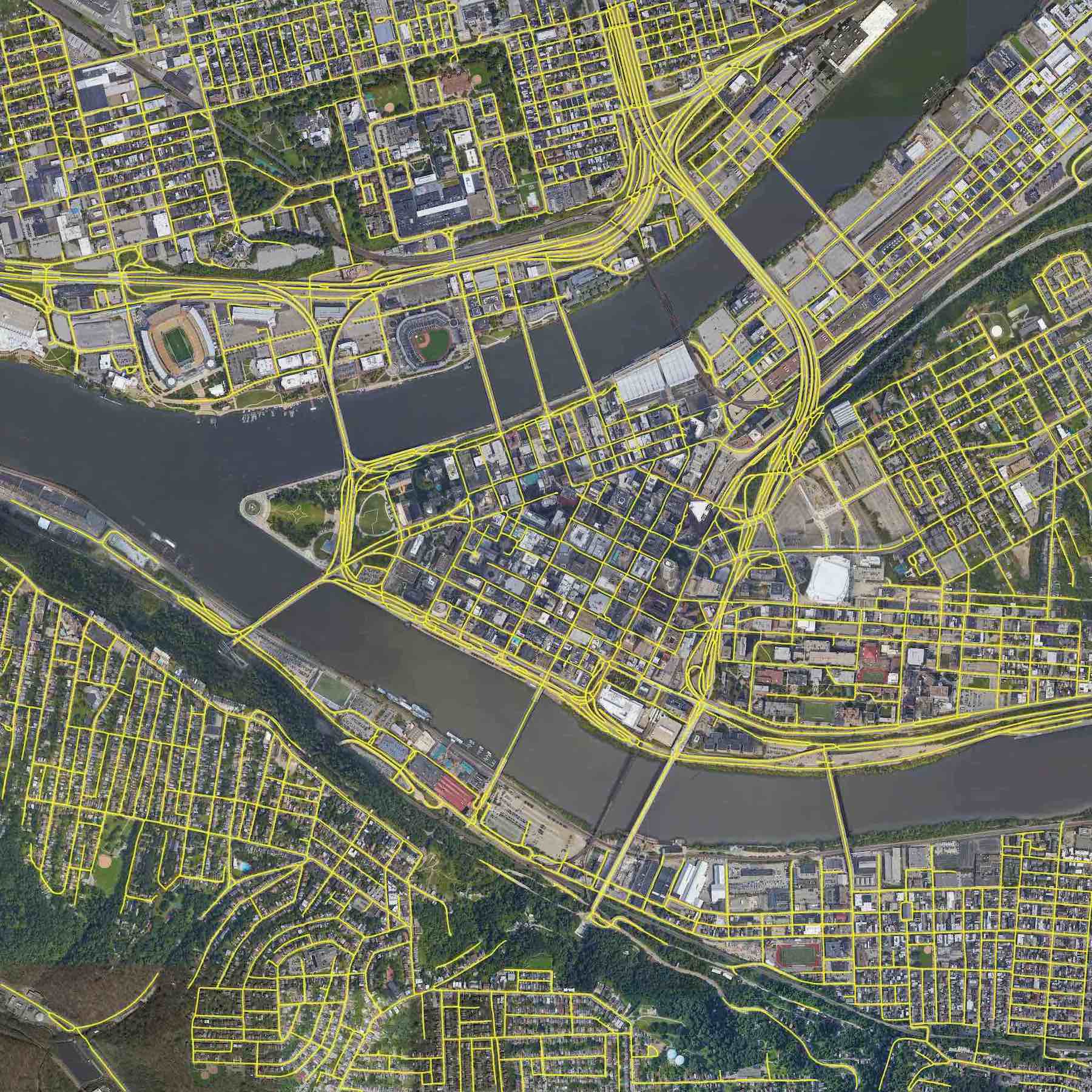
(d) CRESIv2

Figure 10: New York City (top) and Pittsburgh (bottom) Performance. (Left) RoadTracer prediction [8]. (Right) Our CRESIv2 prediction over the same area.

7 Discussion

CRESIv2 improves upon previous methods in extracting road topology from satellite imagery, The reasons for our 5% improvement over the Orientation Learning method applied to SpaceNet data are difficult to pinpoint exactly, but our custom dice + focal loss function (vs the SoftIOU loss of [4]) is a key difference. The enhanced ability of CRESIv2 to disentangle areas of dense road networks accounts for most of the 23% improvement over the RoadTracer method applied to Google satellite imagery + OSM labels.

We also introduce the ability to extract route speeds and travel times. Routing based on time shows only a $3-13\%$ decrease from distance-based routing, indicating that true optimized routing is possible with this approach. The aggregate score of APLS${}_{\rm{time}}=0.64$ implies that travel time estimates will be within $\approx\frac{1}{3}$ of the ground truth.

As with most approaches to road vector extraction, complex intersections are a challenge with CRESIv2. While we attempt to connect gaps based on road heading and proximity, overpasses and onramps remain difficult (Figure 11).

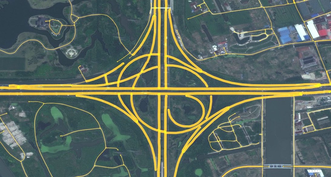
Figure 11: CRESIv2 challenges. While the pixel-based score of this Shanghai prediction is high, correctly connecting roadways in complex intersections remains elusive.

CRESIv2 has not been fully optimized for speed, but even so inference runs at a rate of $280\,{\rm km}^{2}/\,{\rm hour}$ on a machine with a single Titan X GPU. At this speed, a 4-GPU cluster could map the entire $9100\,{\rm km}^{2}$ area of Puerto Rico in $\approx 8$ hours, a significant improvement over the two months required by human labelers [21].

8 Conclusion

Optimized routing is crucial to a number of challenges, from humanitarian to military. Satellite imagery may aid greatly in determining efficient routes, particularly in cases involving natural disasters or other dynamic events where the high revisit rate of satellites may be able to provide updates far more quickly than terrestrial methods.

In this paper we demonstrated methods to extract city-scale road networks directly from remote sensing images of arbitrary size, regardless of GPU memory constraints. This is accomplished via a multi-step algorithm that segments small image chips, extracts a graph skeleton, refines nodes and edges, stitches chipped predictions together, extracts the underlying road network graph structure, and infers speed limit / travel time properties for each roadway. Our code is publicly available at github.com/CosmiQ/cresi.

Applied to SpaceNet data, we observe a 5% improvement over published methods, and when using OSM data our method provides a significant (+23%) improvement over existing methods. Over a diverse test set that includes atypical lighting conditions, off-nadir observation angles, and locales with a multitude of dirt roads, we achieve a total score of APLS${}_{\rm length}=0.67$, and nearly equivalent performance when optimizing for travel time: APLS${}_{\rm time}=0.64$. Inference speed is a brisk $\geq 280\,{\rm km}^{2}\,/\,\rm{hour}/\rm{GPU}$.

While automated road network extraction is by no means a solved problem, the CRESIv2 algorithm demonstrates that true time-optimized routing is possible, with potential benefits to applications such as disaster response where rapid map updates are critical to success.

Acknowledgments We thank Nick Weir, Jake Shermeyer, and Ryan Lewis for their insight, assistance, and feedback.

Appendix A. Road Speed Assignment

See [29] for details on the precise labeling guidelines and road type definitions. We utilize road type (motorway, primary, secondary, tertiary, residential, unclassified, cart track) and road surface type (paved, non-paved) to assign speed to each edge.

Speed is assigned with Table 7, using the Oregon guidelines for road speed [22].

Table 7: Road Speeds (mph)

Road Type	1 Lane	2 Lane	3+ Lane
Motorway	55	55	65
Primary	45	45	55
Secondary	35	35	45
Tertiary	30	30	35
Residential	25	25	30
Unclassified	20	20	20
Cart Track	20	20	20

For each non-paved roadway, the speed from Table 7 is multiplied by 0.75 to give the final speed.

Appendix B. Large Area Test Data

Details of the large are testing regions for SpaceNet data are shown in Table 8, and an example test area displayed in Figure 12.

Table 8: Test Regions

Test Region	Area	Road Length
	(Km2)	(Total Km)
Khartoum$\_0$	3.0	76.7
Khartoum$\_1$	8.0	172.6
Khartoum$\_2$	8.3	128.9
Khartoum$\_3$	9.0	144.4
Las$\_$Vegas$\_0$	68.1	1023.9
Las$\_$Vegas$\_1$	177.0	2832.8
Las$\_$Vegas$\_2$	106.7	1612.1
Paris$\_0$	15.8	179.9
Paris$\_1$	7.5	65.4
Paris$\_2$	2.2	25.9
Shanghai$\_0$	54.6	922.1
Shanghai$\_1$	89.8	1216.4
Shanghai$\_2$	87.5	663.7
Total	608.0	9064.8

Figure 12: SpaceNet road vector labels over Shanghai (purple). The label boundary is discontinuous and irregularly shaped, so we define rectangular regions for testing purposes (e.g.  the blue region denotes test region Shanghai$\_$0).

Appendix C. OSM / SpaceNet Model Comparison

Figure 13 displays comparisons of models trained on OSM data and SpaceNet data.

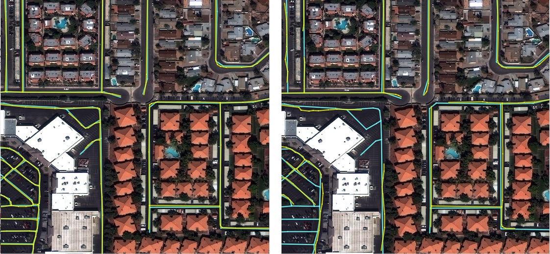
(a)

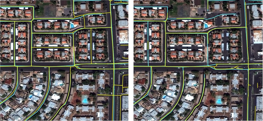
(b)

Figure 13: SpaceNet compared to OSM. Road predictions (yellow) and ground truth SpaceNet labels (blue) for a sample image chips, with SpaceNet models on the left and OSM-trained models on the right. Top: SpaceNet model predictions (left) score APLS${}_{\rm{length}}=0.60$, while OSM model predictions (right) yield APLS${}_{\rm{length}}=0.48$. Bottom: SpaceNet model predictions (left) score APLS${}_{\rm{length}}=0.92$, while OSM model predictions (right) yield APLS${}_{\rm{length}}=0.37$.

Appendix D. CRESIv2 Road Speed Plots

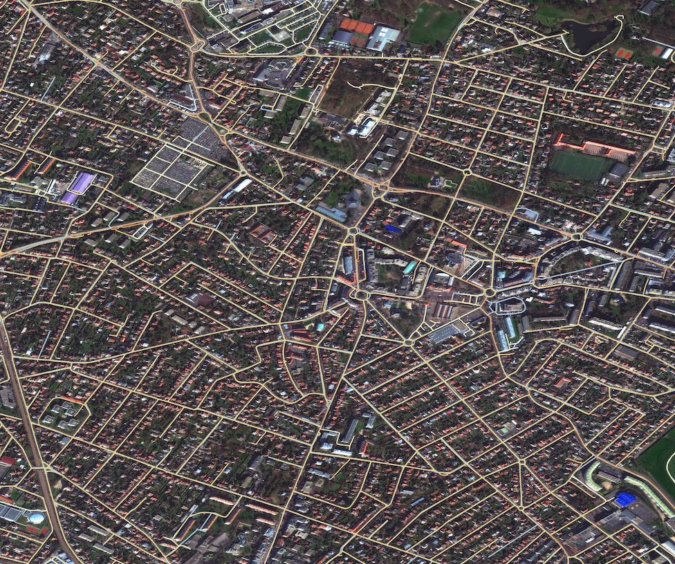
(a)

(b)

Figure 14: Road speed. Output of CRESIv2 inference as applied to large SpaceNet test regions (from top: Paris, Shanghai). Roads are colored by inferred speed limit, from yellow (20 mph) to red (65 mph), with ground truth in gray.

Appendix E. CRESIv2 / RoadTracer Visual Comparison

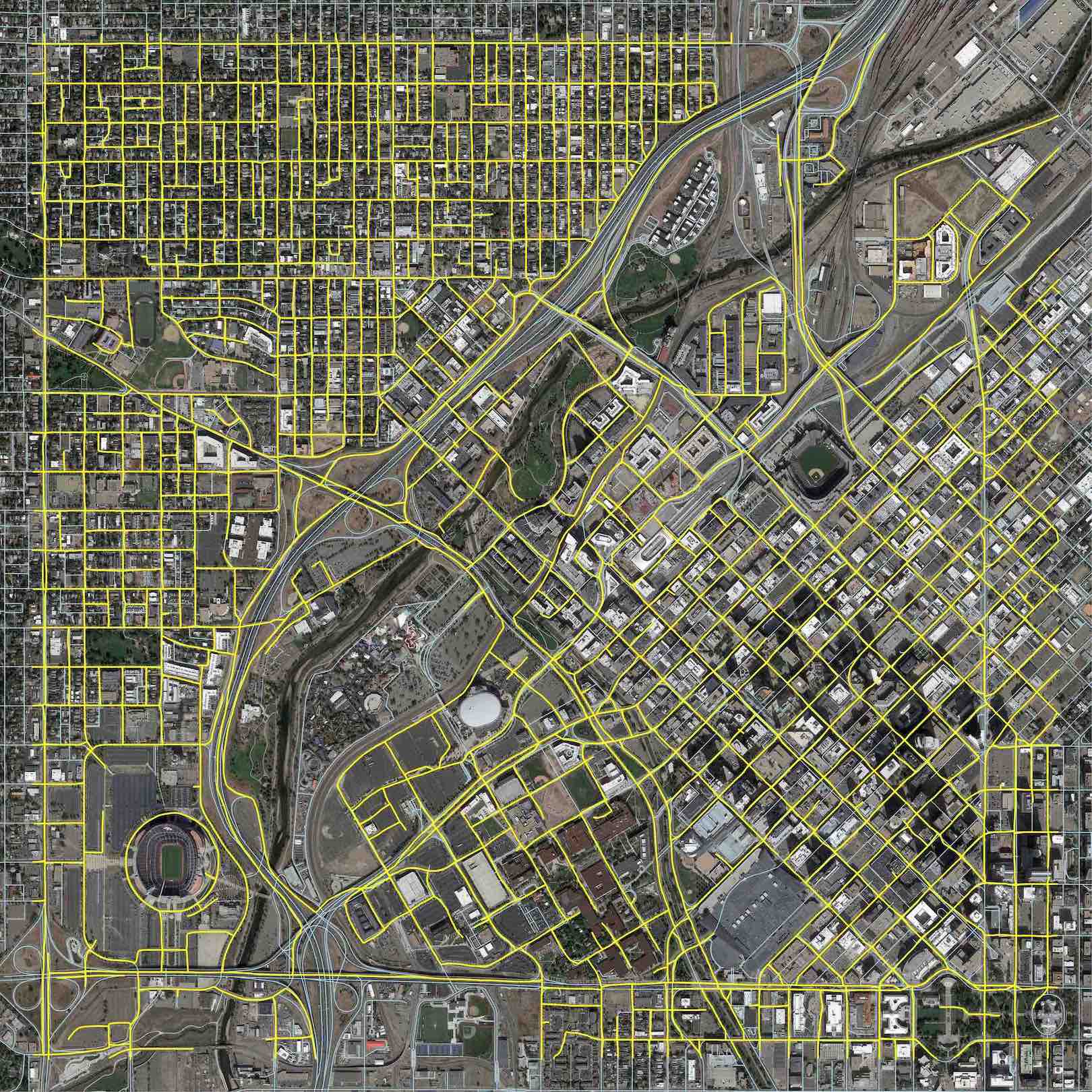
(a)

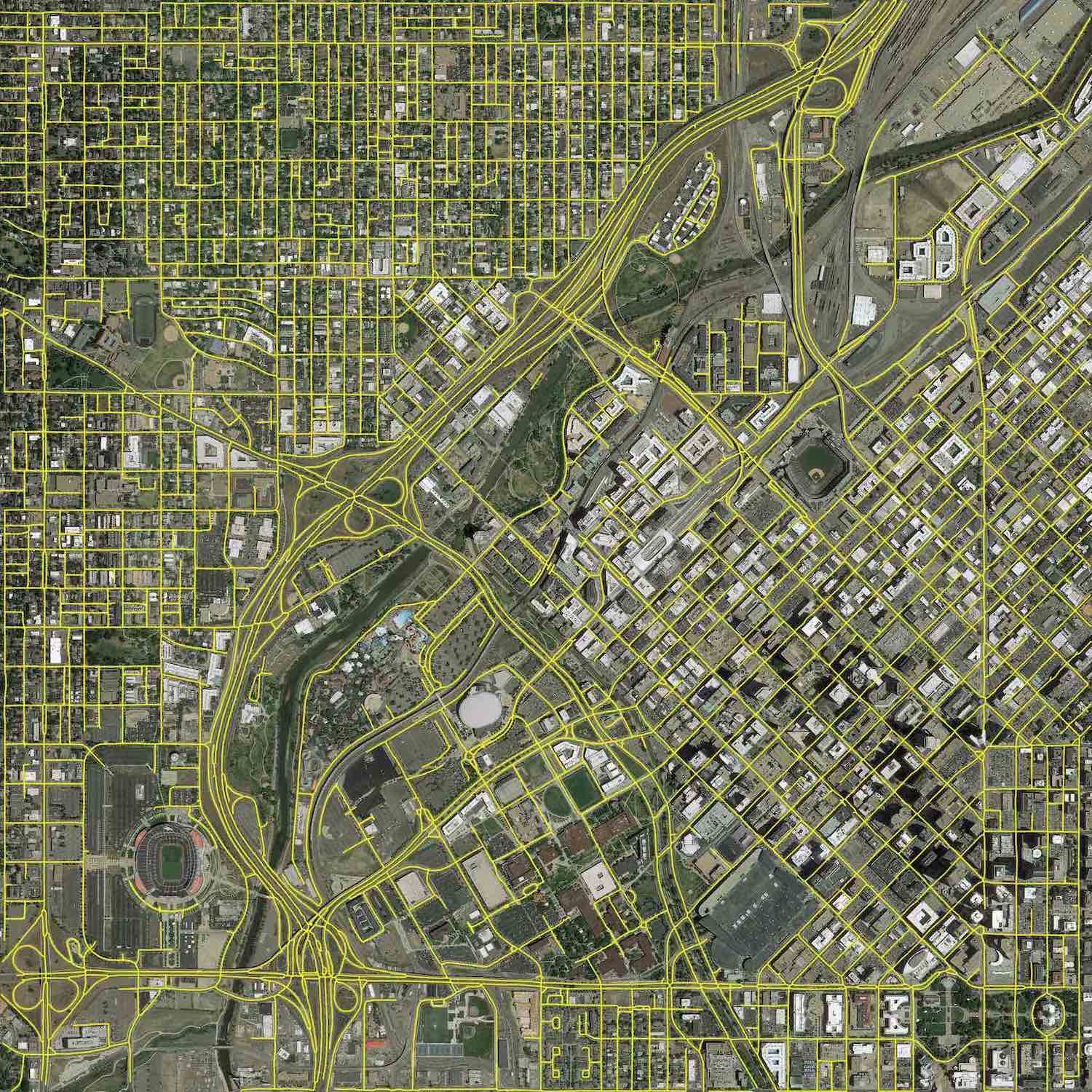
(b)

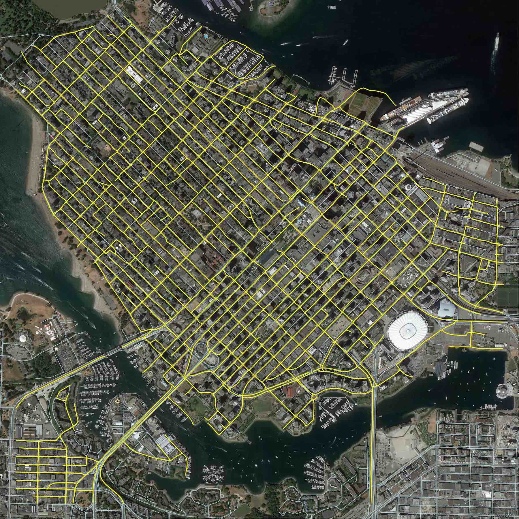
(c)

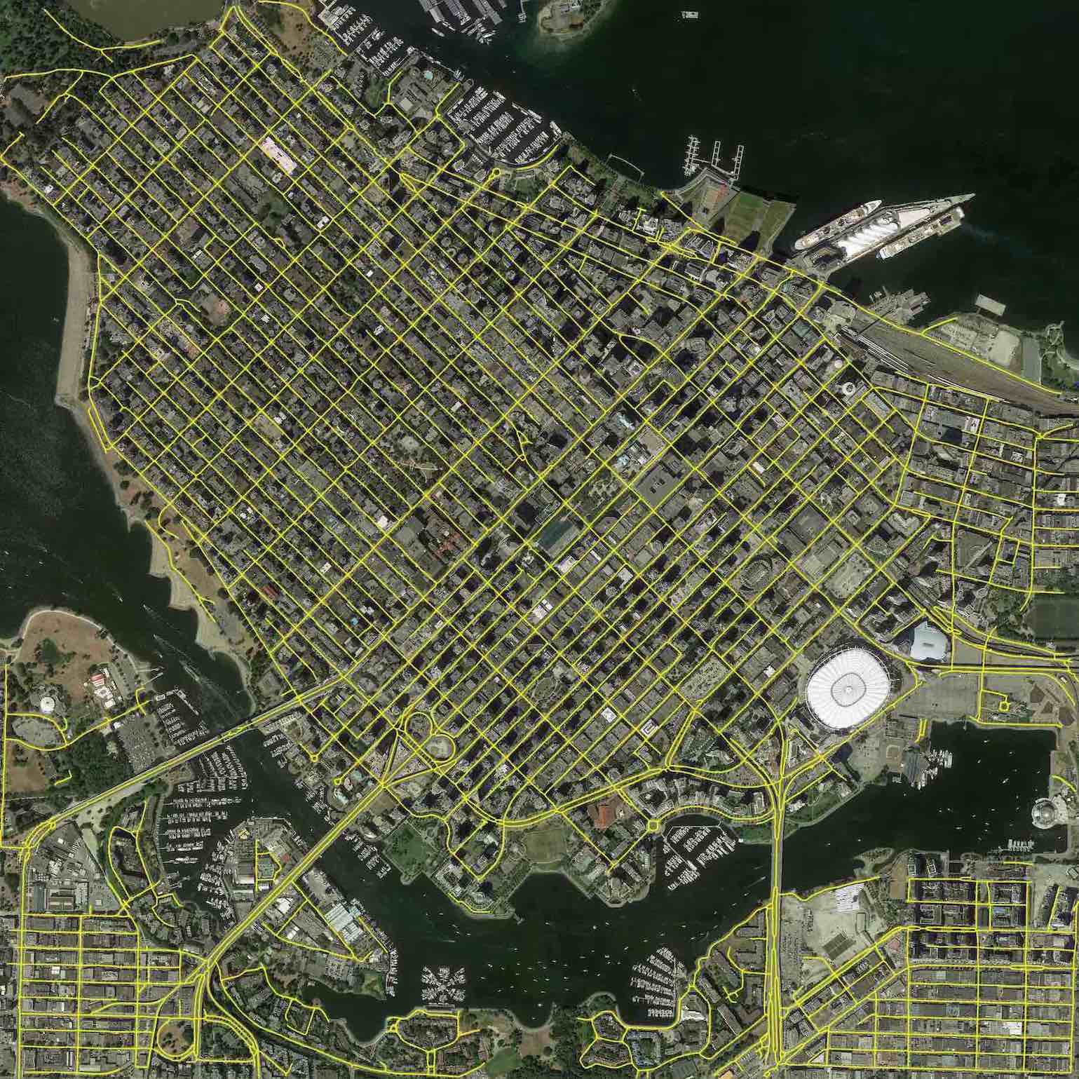
(d)

Figure 15: RoadTracer / CRESIv2. Performance comparison between RoadTracer (left column, OSM labels in gray, predictions in yellow [8]) and CRESIv2 (right column, predictions in yellow) for various cities. From top: Denver, Vancouver.

Appendix F. RoadTracer / CRESIv2 / DeepRoadMapper Zooms

A qualitative comparison of three methods over various cities is shown in Figure 16.

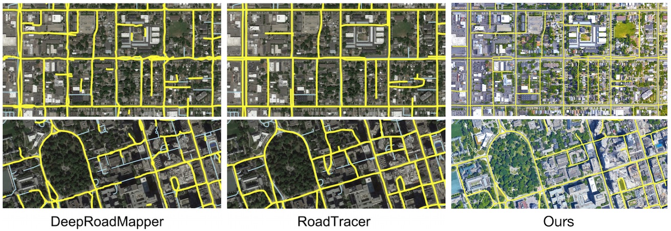
Figure 16: Qualitative comparison of three methods over various cities, (see Figure 10 of [3]).

References

- [1] albu. Spacenet round 3 winner: albu’s implementation. https://github.com/SpaceNetChallenge/RoadDetector/tree/master/albu-solution, 2018.
- [2] F. Bastani. fbastani spacenet solution. https://github.com/SpaceNetChallenge/RoadDetector/tree/master/fbastani-solution, 2018.
- [3] F. Bastani, S. He, M. Alizadeh, H. Balakrishnan, S. Madden, S. Chawla, S. Abbar, and D. DeWitt. RoadTracer: Automatic Extraction of Road Networks from Aerial Images. In Computer Vision and Pattern Recognition (CVPR), Salt Lake City, UT, June 2018.
- [4] A. Batra, S. Singh, G. Pang, S. Basu, C. Jawahar, and M. Paluri. Improved road connectivity by joint learning of orientation and segmentation. In The IEEE Conference on Computer Vision and Pattern Recognition (CVPR), June 2019.
- [5] J. Biagioni and J. Eriksson. Inferring road maps from global positioning system traces: Survey and comparative evaluation. Transportation Research Record, 2291(1):61–71, 2012.
- [6] D. Chai, W. Förstner, and F. Lafarge. Recovering line-networks in images by junction-point processes. In 2013 IEEE Conference on Computer Vision and Pattern Recognition, pages 1894–1901, June 2013.
- [7] CosmiQWorks. Broad area satellite imagery semantic segmentation. https://github.com/CosmiQ/basiss, 2018.
- [8] M. CSAIL. Roadtracer: Automatic extraction of road networks from aerial images. https://roadmaps.csail.mit.edu/roadtracer/, 2018.
- [9] I. Demir, K. Koperski, D. Lindenbaum, G. Pang, J. Huang, S. Basu, F. Hughes, D. Tuia, and R. Raska. Deepglobe 2018: A challenge to parse the earth through satellite images. In 2018 IEEE/CVF Conference on Computer Vision and Pattern Recognition Workshops (CVPRW), pages 172–17209, June 2018.
- [10] A. V. Etten. City-scale road extraction from satellite imagery. CoRR, abs/1904.09901, 2019.
- [11] A. A. Hagberg, D. A. Schult, and P. J. Swart. Exploring network structure, dynamics, and function using networkx. In G. Varoquaux, T. Vaught, and J. Millman, editors, Proceedings of the 7th Python in Science Conference, pages 11 – 15, Pasadena, CA USA, 2008.
- [12] K. He, X. Zhang, S. Ren, and J. Sun. Deep residual learning for image recognition. In 2016 IEEE Conference on Computer Vision and Pattern Recognition (CVPR), pages 770–778, June 2016.
- [13] ISPRS. 2d semantic labeling contest. http://www2.isprs.org/commissions/comm3/wg4/semantic-labeling.html, 2018.
- [14] T. Lin, P. Goyal, R. Girshick, K. He, and P. Dollar. Focal loss for dense object detection. IEEE Transactions on Pattern Analysis and Machine Intelligence, pages 1–1, 2018.
- [15] V. Mnih. Machine Learning for Aerial Image Labeling. PhD thesis, University of Toronto, 2013.
- [16] V. Mnih and G. E. Hinton. Learning to detect roads in high-resolution aerial images. In K. Daniilidis, P. Maragos, and N. Paragios, editors, Computer Vision – ECCV 2010, pages 210–223, Berlin, Heidelberg, 2010. Springer Berlin Heidelberg.
- [17] A. Mosinska, P. Márquez-Neila, M. Kozinski, and P. Fua. Beyond the pixel-wise loss for topology-aware delineation. 2018 IEEE/CVF Conference on Computer Vision and Pattern Recognition, pages 3136–3145, 2017.
- [18] G. Máttyus, W. Luo, and R. Urtasun. Deeproadmapper: Extracting road topology from aerial images. In 2017 IEEE International Conference on Computer Vision (ICCV), pages 3458–3466, Oct 2017.
- [19] G. Máttyus, S. Wang, S. Fidler, and R. Urtasun. Enhancing road maps by parsing aerial images around the world. In 2015 IEEE International Conference on Computer Vision (ICCV), pages 1689–1697, Dec 2015.
- [20] G. Máttyus, S. Wang, S. Fidler, and R. Urtasun. Hd maps: Fine-grained road segmentation by parsing ground and aerial images. In 2016 IEEE Conference on Computer Vision and Pattern Recognition (CVPR), pages 3611–3619, June 2016.
- [21] OpenStreetMap. 2017 hurricanes irma and maria. https://wiki.openstreetmap.org/wiki/2017_Hurricanes_Irma_and_Maria, 2017.
- [22] OpenStreetMap. Osm tags for routing/maxspeed. https://wiki.openstreetmap.org/wiki/OSM_tags\_for\_routing/Maxspeed\#United\_States\_of\_America, 01 2019.
- [23] OpenStreetMap contributors. Planet dump retrieved from https://planet.osm.org . https://www.openstreetmap.org, 2019.
- [24] O. Ronneberger, P. Fischer, and T. Brox. U-net: Convolutional networks for biomedical image segmentation. In N. Navab, J. Hornegger, W. M. Wells, and A. F. Frangi, editors, Medical Image Computing and Computer-Assisted Intervention – MICCAI 2015, pages 234–241, Cham, 2015. Springer International Publishing.
- [25] scikit image. Skeletonize. https://scikit-image.org/docs/dev/auto_examples/edges/plot_skeleton.html, 2018.
- [26] A. Sironi, V. Lepetit, and P. Fua. Multiscale centerline detection by learning a scale-space distance transform. In 2014 IEEE Conference on Computer Vision and Pattern Recognition, pages 2697–2704, June 2014.
- [27] R. Stoica, X. Descombes, and J. Zerubia. A gibbs point process for road extraction from remotely sensed images. International Journal of Computer Vision, 57:121–136, 05 2004.
- [28] E. Türetken, F. Benmansour, B. Andres, H. Pfister, and P. Fua. Reconstructing loopy curvilinear structures using integer programming. In 2013 IEEE Conference on Computer Vision and Pattern Recognition, pages 1822–1829, June 2013.
- [29] A. Van Etten, D. Lindenbaum, and T. M. Bacastow. SpaceNet: A Remote Sensing Dataset and Challenge Series. ArXiv e-prints, July 2018.
- [30] J. Wang, Q. Qin, Z. Gao, J. Zhao, and X. Ye. A new approach to urban road extraction using high-resolution aerial image. ISPRS International Journal of Geo-Information, 5(7), 2016.
- [31] S. Wang, M. Bai, G. Máttyus, H. Chu, W. Luo, B. Yang, J. Liang, J. Cheverie, S. Fidler, and R. Urtasun. Torontocity: Seeing the world with a million eyes. CoRR, abs/1612.00423, 2016.
- [32] J. D. Wegner, J. A. Montoya-Zegarra, and K. Schindler. A higher-order crf model for road network extraction. In 2013 IEEE Conference on Computer Vision and Pattern Recognition, pages 1698–1705, June 2013.
- [33] yxdragon. Skeleton network. https://github.com/yxdragon/sknw, 2018.
- [34] Z. Zhang, Q. Liu, and Y. Wang. Road extraction by deep residual u-net. IEEE Geoscience and Remote Sensing Letters, 15:749–753, 2018.
- [35] L. Zhou, C. Zhang, and M. Wu. D-linknet: Linknet with pretrained encoder and dilated convolution for high resolution satellite imagery road extraction. pages 192–1924, 06 2018.