Some algorithms for the mean curvature flow under topological changes

Abstract

This paper considers and proposes some algorithms to compute the mean curvature flow under topological changes. Instead of solving the fully nonlinear partial differential equations based on the level set approach, we propose some minimization algorithms based on the phase field approach. It is well known that zero-level set of the Allen-Cahn equation approaches the mean curvature flow before the onset of the topological changes; however, there are few papers systematically studying the evolution of the mean curvature flow under the topological changes. There are three main contributions of this paper. First, in order to consider various random initial conditions, we design several benchmark problems with topological changes, and we find different patterns of the evolutions of the solutions can be obtained if the interaction length (width of the interface) is slightly changed, which is different from the problems without topological changes. Second, we propose an energy penalized minimization algorithm which works very well for these benchmark problems, and thus furthermore, for the problems with random initial conditions. Third, we propose a multilevel minimization algorithm. This algorithm is shown to be more tolerant of the unsatisfying initial guess when there are and there are no topological changes in the evolutions of the solutions.

1 Introduction

The moving interface problems refer to a type of problems with interfaces which move in point-wise velocity. Among various kinds of moving interface problems, the mean curvature flow is the most basic and important one. It is defined to be the case when the outward normal velocity is equal to the negative point-wise mean curvature, i.e.,

$$V_{n}(x,t)=-H(x,t)\qquad x\in\Gamma_{t},$$ (1)

where $V_{n}(x,t)$ and $H(x,t)$ denote the outward normal velocity and the mean curvature of the interface $\Gamma_{t}$ respectively. The moving interface problems have been broadly applied to a few different areas such as fluid mechanics, gas dynamics, biology, financial mathematics, etc. There are basically two approaches to formulate the moving interface problems. The first approach is the direct approach, i.e., it tracks the interface directly, including the parametric finite element method barrett2007parametric , the volume of fluid method hirt1981volume , the immersed boundary method peskin2002immersed , the front tracking method unverdi1992front , the immersed interface method leveque1994immersed , and so on. The second approach is the indirect approach, i.e., it seeks another quantity instead of tracking the interface directly, including the level set method osher1988fronts and the phase field method rayleigh1892xx . The biggest advantage of the second approach is that it can easily handle the topological changes compared to the first approach.

The objective of the second approach is to seek an indirect quantity called the level set function (the level set method) or the phase field function (the phase field method). The level set formulation of the mean curvature flow (1) can be written as chen1991uniqueness ; evans1992phase ; evans1992motion

$$\omega_{t} =\Delta\omega-\frac{D^{2}\omega\nabla\omega\cdot\nabla\omega}{|\nabla\omega|^{2}},$$ (2)

$$\omega(\cdot,0) =\omega_{0}(\cdot),$$ (3)

where $D^{2}\omega$ denotes the Hessian of $\omega$ and $\omega_{0}$ satisfies $\Gamma_{0}=\{x\in\mathbb{R}^{d};\ \omega_{0}(x)=0\}(d=2,3)$. This means the interface $\Gamma_{t}$ evolved by the mean curvature flow is the zero-level set of the solution $\omega$. It is explained in evans1992motion that problem (2)–(3) has a unique continuous solution and the level set of $\omega$ evolves according to the mean curvature flow. Some numerical methods are proposed to discretize (2)–(3) in deckelnick2003numerical ; m2017approximations ; kovacs2018convergent ; walkington1996algorithms . The phase field formulation of the mean curvature flow (1) is the singular perturbation of the heat equation called the Allen-Cahn equation with the following initial and boundary conditions

$$u_{t}-\Delta u+\frac{1}{\epsilon^{2}}f(u) =0 \qquad\mbox{in }\Omega_{T}:=\Omega\times(0,T),$$ (4)

$$\frac{\partial u}{\partial n} =0 \qquad\mbox{in }\partial\Omega_{T}:=\partial\Omega\times(0,T),$$ (5)

$$u =u_{0} \qquad\mbox{in }\Omega\times\{t=0\}.$$ (6)

where $\epsilon$ denotes the interaction length, $\Omega\subseteq\mathbb{R}^{d}$ is a bounded domain, $f=F^{\prime}$ for some double well potential function $F$, and $F(u)=\frac{1}{4}(u^{2}-1)^{2}$ is used in this paper. The zero-level sets of $u$ are proved to converge to the mean curvature flow in evans1992phase ; ilmanen1993convergence , and the zero-level sets of numerical solutions are proved to converge to the mean curvature flow in Feng_Prohl03 ; Feng_Wu05 ; feng2014analysis ; kessler2004posteriori ; li2015numerical ; xu2019stability . We refer the readers to further numerical discussions on the stochastic mean curvature flow feng2014finite ; feng2017finite ; feng2018strong ; majee2018optimal and the Hele-Shaw flow feng2016analysis ; li2017error ; wu2018analysis which is an another fundamental moving interface problem.

The above results discuss the evolutions of the solutions without topological changes. In bartels2011quasi ; bartels2011robust ; bartels2010lower , the authors consider the topological changes under some initial conditions, but the evolutions of the solutions behave similarly under different values of the interaction length. In du2005retrieving , the authors suggest using Euler number to retrieve topological information thus to avoid unphysical changes of the topology. Different from the above results, this paper considers some sensitive benchmark initial conditions, i.e. the topology or the patterns of the evolutions of the solutions could be totally different under different values of the interaction length. The motivation of investigating these sensitive initial conditions is that they frequently happen when the initial conditions are random or rough. In this paper, we assume there is no fattening phenomenon cesaroni2018fattening ; evans1992motion ; ilmanen1993convergence in the evolutions of the solutions under specially designed initial conditions. The objectives of this paper are threefold. First, the random initial conditions can be used to test the topological changes in the worst scenarios, so this paper constructs and solves several these kinds of sensitive benchmark problems, and finally tests the random initial conditions. Second, this paper proposes an energy penalized minimization algorithm which is aimed to accurately track the mean curvature flow under topological changes and efficiently solve the problem, i.e., it allows big time step size compared to classical numerical methods for the phase field models. All the proposed benchmark problems as well as the problems with random initial conditions will be used to validate this algorithm. Third, a multilevel minimization algorithm is proposed to handle bad initial guesses and the topological changes. The objective of this algorithm is to construct convex functionals such that their minimization problems do not significantly depend on the initial guesses.

This paper has four additional sections. In section 2, we construct several benchmark problems with topological changes. The level set method, the phase field method, and the energy minimization method (without penalty) are used to compare the evolutions of the solutions. In section 3, we propose the energy penalized minimization algorithm. This algorithm is implemented for the aforementioned benchmark problems as well as problems with random initial conditions. In section 4, we propose a multilevel minimization algorithm. Some examples with and without topological changes are used to justify this algorithm. In section 5, we give a short concluding remark to summarize the results in this paper.

2 Some Benchmark Problems.

In this section, we will state a few benchmark problems of the mean curvature flow under topological changes. The level set method, the energy minimization method, and the phase field method are employed in this section. The solution computed by the level set method is considered the reference solution. We begin with the discretization of the phase field model. We first introduce some notations. Let $\mathcal{T}_{h}$ be a shape-regular triangulation of $\Omega\subset\mathbb{R}^{d}\ (d=2,3)$, $K\in\mathcal{T}_{h}$ represent each element, and $h$ denote the diameter of $K$. Define the finite element space $V_{h}$ by

$$V_{h}=\bigl{\{}v_{h}\in C(\overline{\Omega}):\ v_{h}|_{K}\in P_{r}(K)\bigr{\}},$$ (7)

where $C(\overline{\Omega})$ denotes the set of all continuous functions on $\overline{\Omega}$ and $P_{r}(K)$ denotes the set of all polynomials whose degrees are less than or equal to a given positive integer $r$ on $K$. Let $k$ be the time step size, $\|\cdot\|_{L^{2}}$ be the $L^{2}$-norm, and $(\cdot,\cdot)$ be the $L^{2}$-inner product over the domain $\Omega$. The uniform time step size $k$ can be extended to non-uniform time step size $k_{n}$, $n=1,2,\cdots$ in this paper. The first well-known scheme is the standard first-order fully implicit scheme (FIS), which is defined by seeking $u_{h}^{n}\in V_{h}$ for $n=1,2,\cdots$, such that

$$(\frac{u_{h}^{n}-u_{h}^{n-1}}{k},v_{h})+(\nabla u_{h}^{n},\nabla v_{h})+\frac{1}{\epsilon^{2}}((u_{h}^{n})^{3}-u_{h}^{n},v_{h})=0\qquad\forall v_{h}\in V_{h}.$$ (8)

The following are some usual numerical schemes which will be used in this paper. The convex splitting scheme is to find $u_{h}^{n}\in V_{h}$ for $n=1,2,\cdots$, such that

$$(\frac{u_{h}^{n}-u_{h}^{n-1}}{k},v_{h})+(\nabla u_{h}^{n},\nabla v_{h})+\frac{1}{\epsilon^{2}}((u_{h}^{n})^{3}-u_{h}^{n-1},v_{h})=0\qquad\forall v_{h}\in V_{h}.$$ (9)

The Semi-implicit scheme is to find $u_{h}^{n}\in V_{h}$ for $n=1,2,\cdots$, such that

$$(\frac{u_{h}^{n}-u_{h}^{n-1}}{k},v_{h}) +(\nabla u_{h}^{n},\nabla v_{h})$$ (10)

$$+\frac{1}{\epsilon^{2}}((u_{h}^{n-1})^{3}-u_{h}^{n-1},v_{h})=0\qquad\forall v_{h}\in V_{h}.$$

The modified Crank-Nicolson scheme is to find $u_{h}^{n}\in V_{h}$ for $n=1,2,\cdots$, such that

$$\bigl{(}\frac{u_{h}^{n}-u_{h}^{n-1}}{k},v_{h}\bigr{)} +\bigl{(}\frac{\nabla u_{h}^{n}+\nabla u_{h}^{n-1}}{2},\nabla v_{h}\bigr{)}$$ (11)

$$+\frac{1}{\epsilon^{2}}(\tilde{F}[u_{h}^{n},u_{h}^{n-1}],v_{h})=0\quad\forall v_{h}\in V_{h},$$

where

$$\tilde{F}[u,u_{h}^{n-1}]=\begin{cases}\frac{F(u)-F(u_{h}^{n-1})}{u-u_{h}^{n-1}}&u\neq u^{n-1}_{h},\\ u^{3}-u&u=u^{n-1}_{h}.\end{cases}$$

A review of different numerical schemes can also be found in shen2011spectral , and a few benchmark problems can be found in church2019high .

Next we define the following free-energy functional $J_{\epsilon}^{\rm AC}$ and the discrete energy $E_{n}^{\rm AC}$

$$J_{\epsilon}^{\rm AC}(v) :=\int_{\Omega}\Bigl{(}\frac{1}{2}|\nabla v|^{2}+\frac{1}{\epsilon^{2}}F(v)\Bigr{)}\,dx,$$ (12)

$$E_{n}^{\rm AC}(u_{h};u_{h}^{n-1}) :=J_{\epsilon}^{\rm AC}(u_{h})+\frac{1}{2k}\int_{\Omega}(u_{h}-u_{h}^{n-1})^{2}dx.$$ (13)

It is known that the Allen-Cahn equation is the $L^{2}$-gradient flow of the functional $J_{\epsilon}^{\rm AC}$, and it is proved that the fully implicit scheme (8) is equivalent to the following energy minimization problem:

$$u_{h}^{n}=\underset{u_{h}\in V_{h}}{\mathrm{argmin}}E_{n}^{\rm AC}(u_{h};u_{h}^{n-1}).$$ (14)

See xu2019stability for the relations between other numerical schemes and the energy minimization methods.

When there are no topological changes, it was numerically observed in feng2014analysis ; li2015numerical ; zhang2009numerical that the energy decays slowly. When there are topological changes, it was numerically observed that the energy decays fast. It is very hard or even impossible to calculate the exact energy especially when the geometry is complex. Here we provide an energy equality to formally explain the above observations; i.e., when topological changes happen, the term $k\sum_{n=0}^{\ell}R^{n}_{\epsilon}$ in Theorem 2.1 is larger since the profile of the solutions change more. Note the discrete energy inequality of the Allen-Cahn equation was established in feng2014analysis ; xu2019stability .

Theorem 2.1

Let $u_{h}^{n}$ be a solution of scheme (8) and define the difference operator $d_{t}$ by

$$d_{t}u^{m}:=\frac{u^{m}-u^{m-1}}{k},m=1,2,\cdots,M,$$

where $M$ is the largest positive integer less than or equal to $\frac{T}{k}$. Then the following discrete energy equality holds:

$$J_{\epsilon}^{AC}(u_{h}^{\ell})+k\sum_{n=0}^{\ell}R^{n}_{\epsilon}=J_{\epsilon}^{AC}(u_{h}^{0})\qquad\text{for }0\leq\ell\leq M,$$

where the functional $J_{\epsilon}^{\rm AC}$ is defined in (12), and $R^{n}_{\epsilon}$ is defined by

$$R^{n}_{\epsilon}:=\Bigl{(}1-\frac{k}{2\epsilon^{2}}\Bigr{)}\|d_{t}u_{h}^{n}\|_{L^{2}}^{2}+\frac{k}{2}\|\nabla d_{t}u_{h}^{n}\|_{L^{2}}^{2}+\frac{k}{4\epsilon^{2}}\|d_{t}(u_{h}^{n})^{2}\|_{L^{2}}^{2}+\frac{k}{2\epsilon^{2}}\|u_{h}^{n}d_{t}u_{h}^{n}\|_{L^{2}}^{2}.$$

Proof

Choosing $v_{h}=u_{h}^{n}-u_{h}^{n-1}$ in (8), we get

$$\frac{1}{k}\|u_{h}^{n}-u_{h}^{n-1}\|_{L^{2}}^{2}+(\nabla u_{h}^{n},\nabla(u_{h}^{n}-u_{h}^{n-1}))+\frac{1}{\epsilon^{2}}((u_{h}^{n})^{3}-u_{h}^{n},u_{h}^{n}-u_{h}^{n-1})=0.$$ (15)

Define the backward difference operator

$$d_{t}v^{m}:=\frac{v^{m}-v^{m-1}}{k}\qquad\forall m=1,2,\cdots,\ell.$$ (16)

Note the following identities

$$(\nabla u_{h}^{n},\nabla(u_{h}^{n}-u_{h}^{n-1}))= \frac{1}{2}\|\nabla u_{h}^{n}\|_{L^{2}}^{2}-\frac{1}{2}\|\nabla u_{h}^{n-1}\|_{L^{2}}^{2}$$ (17)

$$+\frac{1}{2}\|\nabla(u_{h}^{n}-u_{h}^{n-1})\|_{L^{2}}^{2},$$

$$((u_{h}^{n})^{3}-u_{h}^{n},u_{h}^{n}-u_{h}^{n-1})= \frac{k}{4}d_{t}\|(u_{h}^{n})^{2}-1\|_{L^{2}}^{2}+\frac{k^{2}}{4}\|d_{t}(u_{h}^{n})^{2}\|_{L^{2}}^{2}$$ (18)

$$+\frac{k^{2}}{2}\|u_{h}^{n}d_{t}u_{h}^{n}\|_{L^{2}}^{2}-\frac{k^{2}}{2}\|d_{t}u_{h}^{n}\|_{L^{2}}^{2}.$$

Then we have

$$k\|d_{t}u_{h}^{n}\|_{L^{2}}^{2}+\frac{1}{2}\|\nabla u_{h}^{n}\|_{L^{2}}^{2}-\frac{1}{2}\|\nabla u_{h}^{n-1}\|_{L^{2}}^{2}+\frac{1}{2}\|\nabla(u_{h}^{n}-u_{h}^{n-1})\|_{L^{2}}^{2}$$ (19)

$$\qquad+\frac{k}{4\epsilon^{2}}d_{t}\|(u_{h}^{n})^{2}-1\|_{L^{2}}^{2}+\frac{k^{2}}{4\epsilon^{2}}\|d_{t}(u_{h}^{n})^{2}\|_{L^{2}}^{2}$$

$$\qquad+\frac{k^{2}}{2\epsilon^{2}}\|u_{h}^{n}d_{t}u_{h}^{n}\|_{L^{2}}^{2}-\frac{k^{2}}{2\epsilon^{2}}\|d_{t}u_{h}^{n}\|_{L^{2}}^{2}=0.$$

Taking the summation on both sides of (19) over $n$ from $0$ to $\ell$ yields the conclusion.

In the following tests, we compare the evolutions of the solutions of different numerical schemes, and the evolutions of the solutions of different methods such as the level set method, the phase field method and the energy minimization method. Specifically, in Test 1, we verify that all these popular numerical schemes behave similarly as long as the time step size is small enough. Therefore, we choose the fully implicit scheme in the following tests; in Test 2, we choose two circles with a larger distance, and we observe that these three methods behave similarly; in Test 3, we choose two circles with a smaller distance, then the solution of the level set method separates, but the solutions of the phase field method and the energy minimization method merge unless $\epsilon$ is very small, in which case the computational cost is large (some spatial grids should be placed iniside the diffuse interface); in Test 4, we choose another wedge-like initial condition, then the solution of the level set method merges, but the solutions of the phase field method and the energy minimization method separate unless $\epsilon$ is very small.

Test 1. In this test, we test a benchmark problem with a circle with $radius=0.2$ for the initial condition based on different numerical schemes. Figure 1 shows the change of radius with respect to time for different numerical schemes. As expected, we find that when the time step size is sufficiently small, the evolutions of the solutions are very similar when different numerical schemes are used. Therefore, we just need to use the fully implicit scheme with a small time step size to compute the evolutions of the solutions.

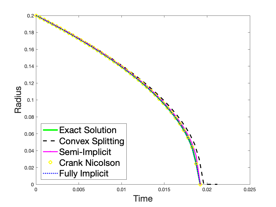
Figure 1: Test 1. Evolutions of the solutions of different numerical schemes

Test 2. In this test, we compare the evolutions of the solutions when the initial condition is two circles with a large distance based on the level set method and the phase field method. In Figure 2, the level set method is used to compute the evolution of the solution, and we find that these two circles separate. The distance between these two circles is $d=0.05$, the spatial size is $h=0.01$, and the time step size is $k=2.5\times 10^{-5}$. In Figure 3, the fully implicit scheme of the phase field method is used to compute the evolution of the solution, and we find that these two circles separate. The distance between these two circles is $d=0.05$, the spatial size is $h=0.008$, the interaction length is $\epsilon=0.01$, and the time step size is $k=1\times 10^{-4}$. In Figure 4, using the same data for Figure 3, the energy minimization method is used to compute the evolution of the solution, and we find that these two circles separate. From this test, we observe that the evolutions of the solutions based on different methods behave similarly. The Figure 5 indicates the energy change over time for both the phase field method and the energy minimization method. This test takes the initial condition used in many other papers, and this test demonstrates that the topological changes need not be considered when the distance between the two circles is large.

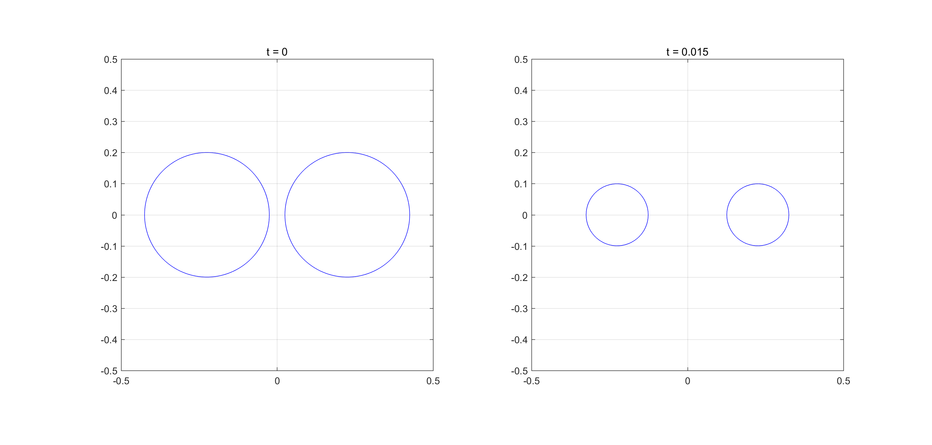
Figure 2: Test 2. The level set method is used. The left graph is the initial condition, and the right graph is the evolution of the solution at $t=0.015$.

Figure 3: Test 2. The phase field method is used. The left graph is the initial condition, and the right graph is the evolution of the solution at $t=0.015$ with $\epsilon=0.01$.

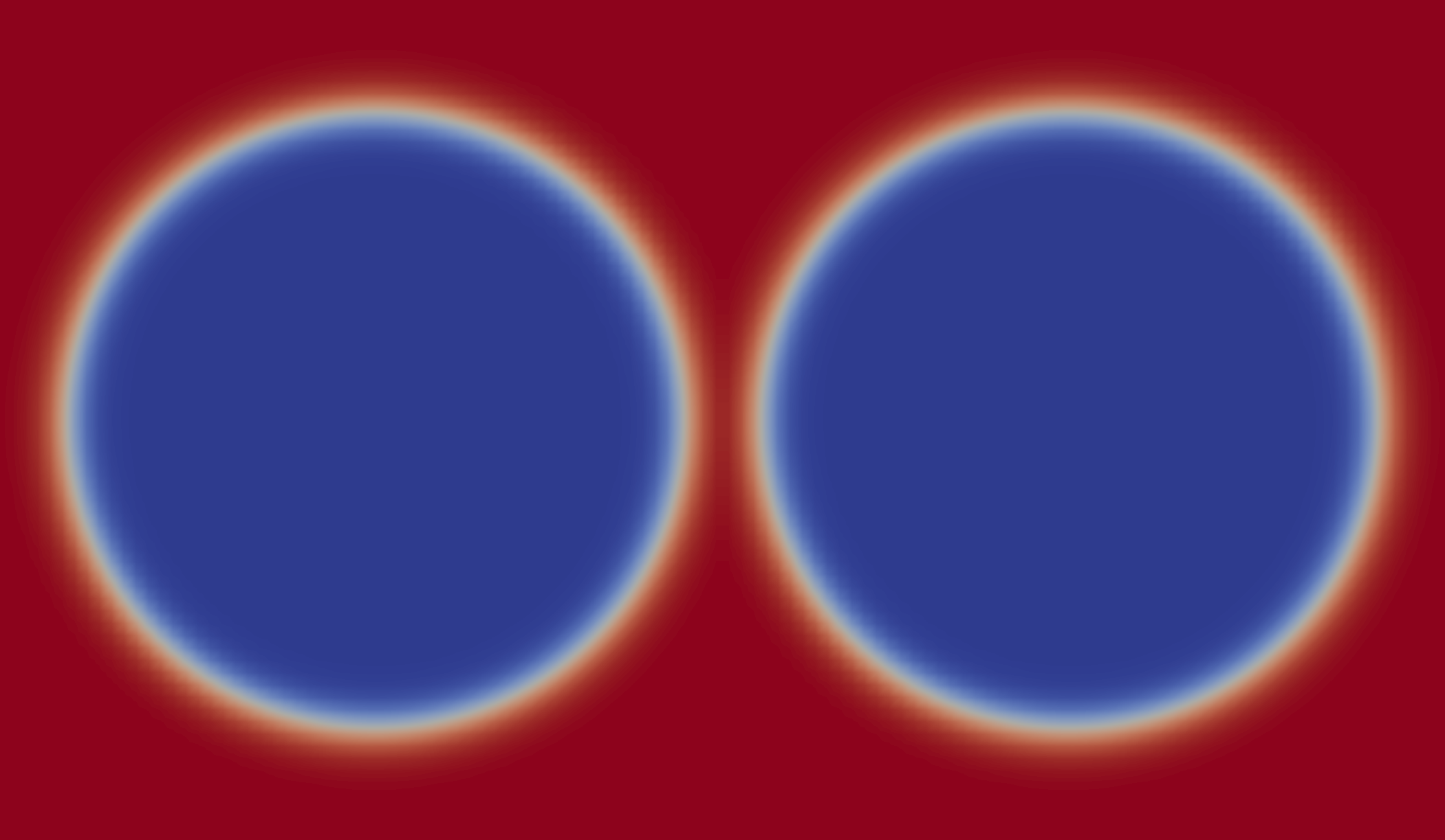
Figure 4: Test 2. The energy minimization method is used. The left graph is the initial condition, and the right graph is the evolution of the solution at $t=0.015$ with $\epsilon=0.01$.

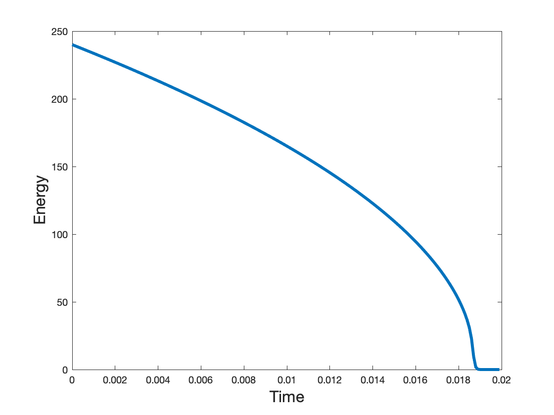
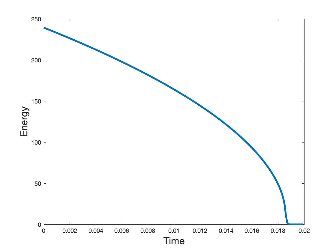
Figure 5: Test 2. The left hand side is the energy of the FIS, and the right hand side is the energy of the energy minimization method with $\epsilon=0.01$.

Test 3. In this test, we compare the evolutions of the solutions when the initial condition is two circles with a small distance based on the level set method, the phase field method, and the energy minimization method. In Figure 6, the level set method is used to compute the evolution of the solution, and we find that these two circles separate. The distance between these two circles is $d=0.02$, the spatial size is $h=0.005$, and the time step size is $k=2.5\times 10^{-6}$. In Figure 7, the fully implicit scheme of the phase field method is used to compute the evolution of the solution, and we find that these two circles merge, which is inconsistent with the result from the level set method. The distance between these two circles is $d=0.02$, the spatial size is $h=0.005$, the interaction length is $\epsilon=0.01$, and the time step size is $k=1\times 10^{-4}$. In Figure 8, using the same data for Figure 7, the energy minimization method is used to compute the evolution of the solution, and we find that these two circles merge, which also contradicts the result of the level set method. Moreover, we tried much smaller time step sizes for the phase field method and the energy minimization method, but these two circles still merge. The Figure 9 indicates the energy change over time for both the phase field method and the energy minimization method. We observe that the energy has a sharp decrease at the beginning, then it decreases slower until around time 0.035. Then, it decreases sharply again until it reaches 0.

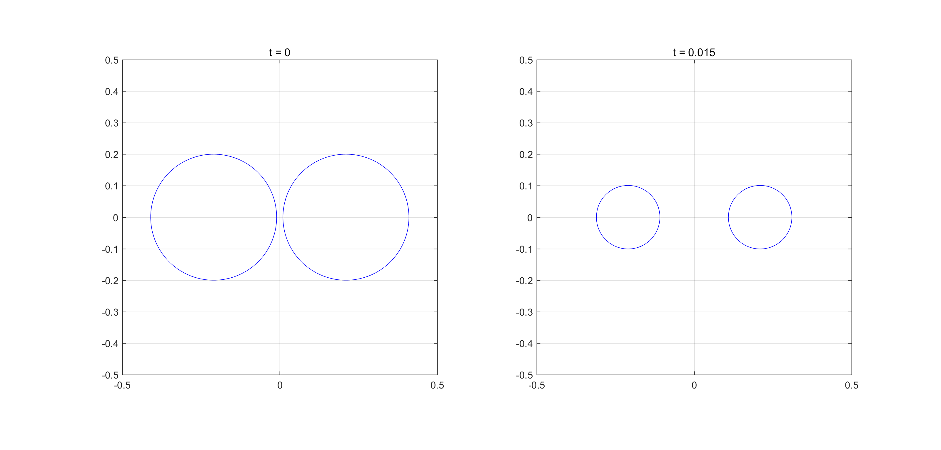
Figure 6: Test 3. The level set method is used. The left graph is the initial condition, and the right graph is the evolution of the solution at $t=0.015$.

Figure 7: Test 3. The phase field method is used. The left graph is the initial condition, and the right graph is the evolution of the solution at $t=0.015$ with $\epsilon=0.01$.

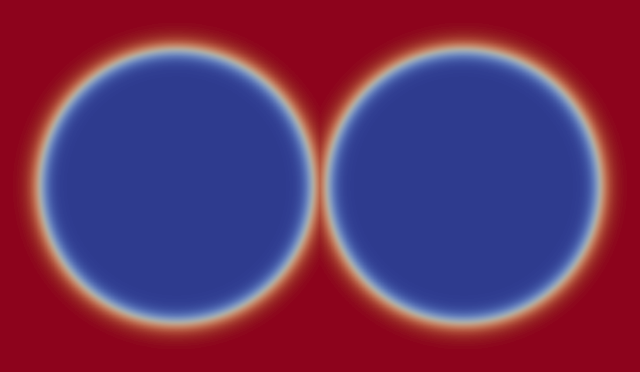
Figure 8: Test 3. The energy minimization method is used. The left graph is the initial condition, and the right graph is the evolution of the solution at $t=0.015$ with $\epsilon=0.01$.

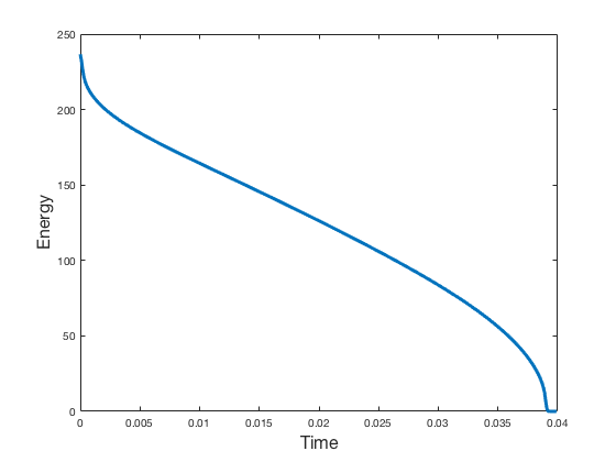
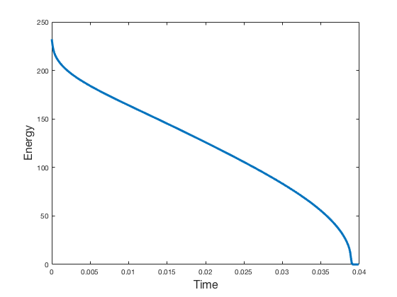
Figure 9: Test 3. The left hand side is the energy of the FIS, and the right hand side is the energy of the energy minimization method with $\epsilon=0.01$.

In Figure 10, the phase field method is used to compute the evolution of the solution, and we find that these two circles separate. The distance between these two circles is $d=0.02$, the spatial size is $h=0.0018$, the interaction length is $\epsilon=0.002$, and the time step size is $k=4\times 10^{-6}$. In Figure 11, using the same data for Figure 10, the energy minimization method is used to compute the evolution of the solution, and we find that these two circles separate. Using a small $\epsilon$, those two methods give very similar results as the level set method. However, with a small $\epsilon$, the required computational cost increases significantly. The Figure 12 indicates the energy change over time for both the phase field method and the energy minimization method. We observe that the energy decreases gradually until time 0.018, and then decreases sharply until it reaches 0. This test validates that the interaction length plays a crucial role for some initial conditions.

Figure 10: Test 3. The phase field method is used. The left graph is the initial condition, and the right graph is the evolution of the solution at $t=0.012$ with $\epsilon=0.002$.

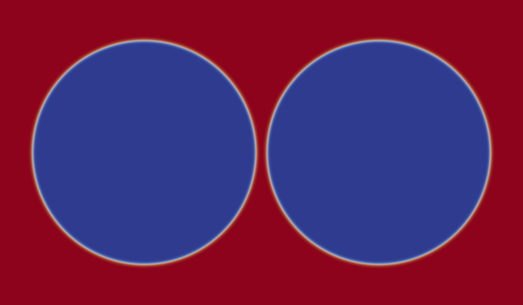
Figure 11: Test 3. The energy minimization method is used. The left graph is the initial condition, and the right graph is the evolution of the solution at $t=0.012$ with $\epsilon=0.002$.

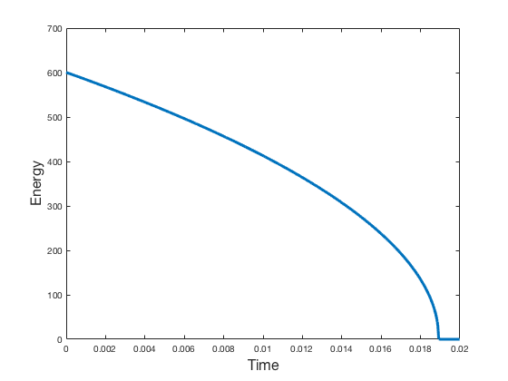
Figure 12: Test 3. The left hand side is the energy of the FIS, and the right hand side is the energy of the energy minimization method with $\epsilon=0.002$.

Test 4. In this test, we compare the evolutions of the solutions when the initial condition is two wedges with small distance connections, based on the level set method, the phase field method, and the energy minimization method. Here the domain $\Omega:=[-0.5,0.5]^{2}$. Define ${\bf m_{1}}=-{\bf m_{3}}:=(0,2)$, ${\bf m_{2}}:=(0,0)$, $M:=0.01$, $r_{1}=r_{3}:=2/3-0.5\times M$, and $r_{2}:=1/3$. Also, set $d_{j}({\bf X}):=|{\bf X}-{\bf m_{j}}|-r_{j}$ for ${\bf X}\in\Omega$, where ${\bf X}=(x,y)$. Then for ${\bf X}\in\Omega$, define

$$d({\bf X}):=\max\{-d_{1}({\bf X}),d_{2}({\bf X}),-d_{3}({\bf X})\},\hskip 17.07182ptu_{0}({\bf X}):=-\tanh(d({\bf X})/\sqrt{2}\times M).$$

Figure 13 shows the evolution of the solution under the above initial condition using the level set method, with spatial size $h=0.005$ and time step $k=6.25\times 10^{-6}$. We observe that the two wedges merge using the level set method. In Figure 14, the phase field method is used to compute the evolution of the solution, and we find that these two wedges separate, which is inconsistent with the result of the level set method. The spatial size is $h=0.005$, the interaction length is $\epsilon=0.01$, and the time step size is $k=1\times 10^{-4}$. In Figure 15, using the same data for Figure 14, the energy minimization method is used to compute the evolution of the solution, and we find that these two wedges separate, which is also inconsistent with the result of the level set method. Figure 16 indicates the energy change over time for both the phase field method and the energy minimization method. We observe that the energy has a sharp drop at the beginning for both methods, then it decreases slowly until around time $3\times 10^{-3}$. Then it decreases faster again until it reaches 0.

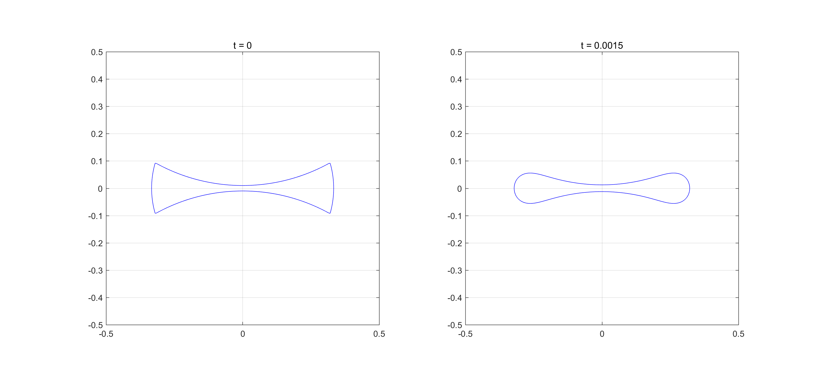
Figure 13: Test 4. The level set method is used. The left graph is the initial condition, and the right graph is the evolution of the solution at $t=0.015$.

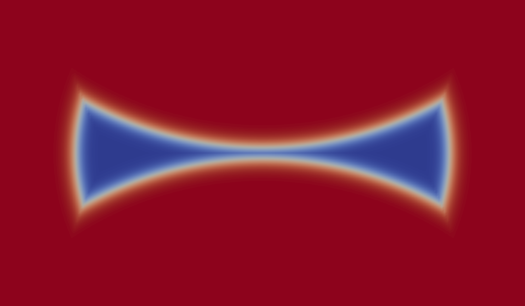
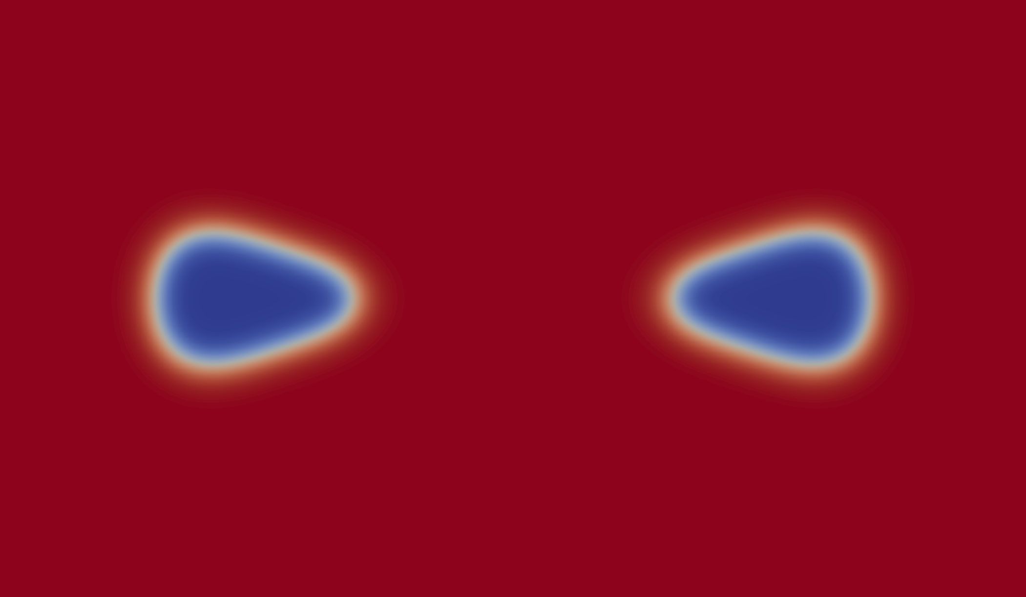
Figure 14: Test 4. The phase field method is used. The left graph is the initial condition, and the right graph is the evolution of the solution at $t=0.001$ with $\epsilon=0.01$.

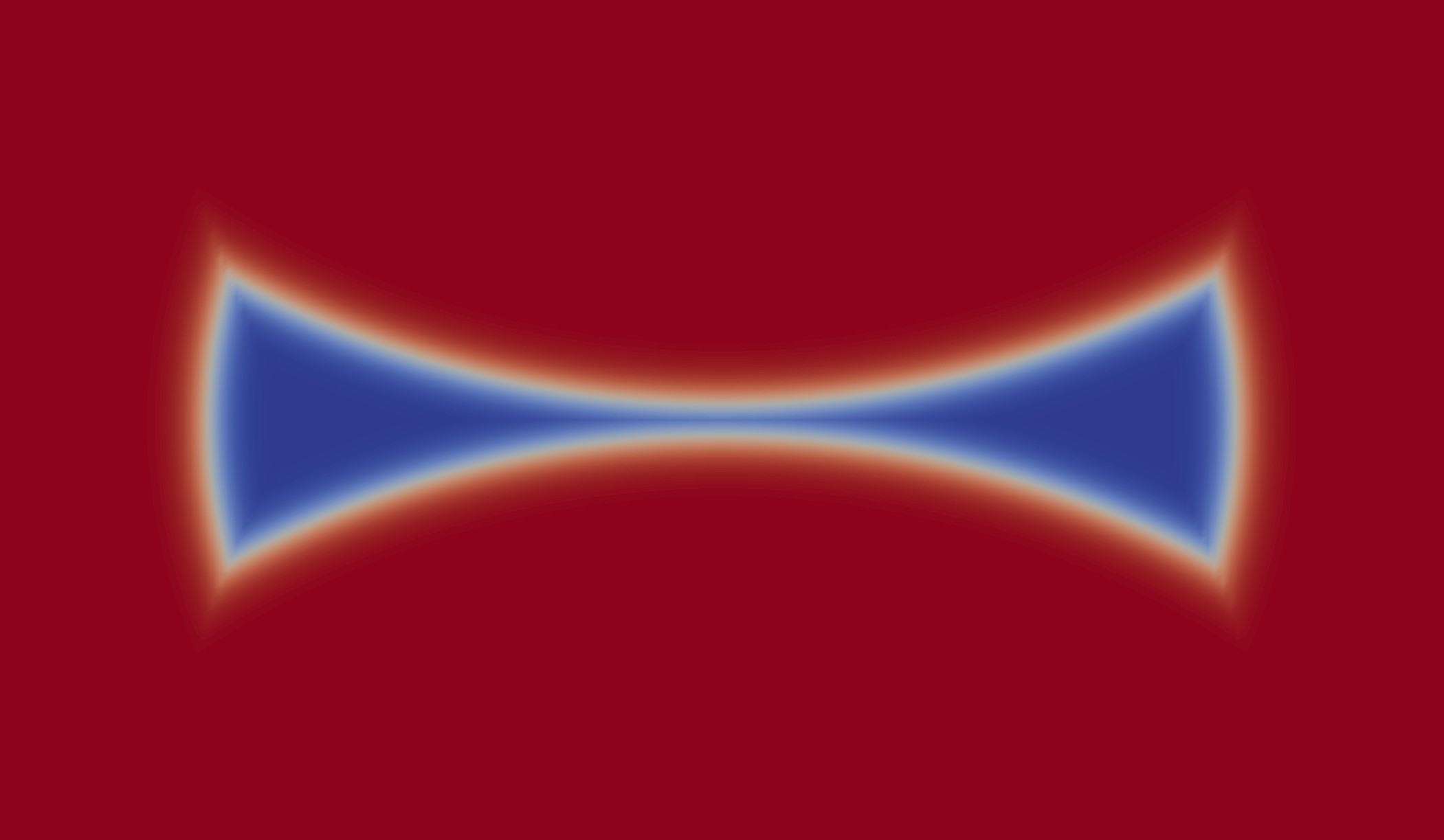
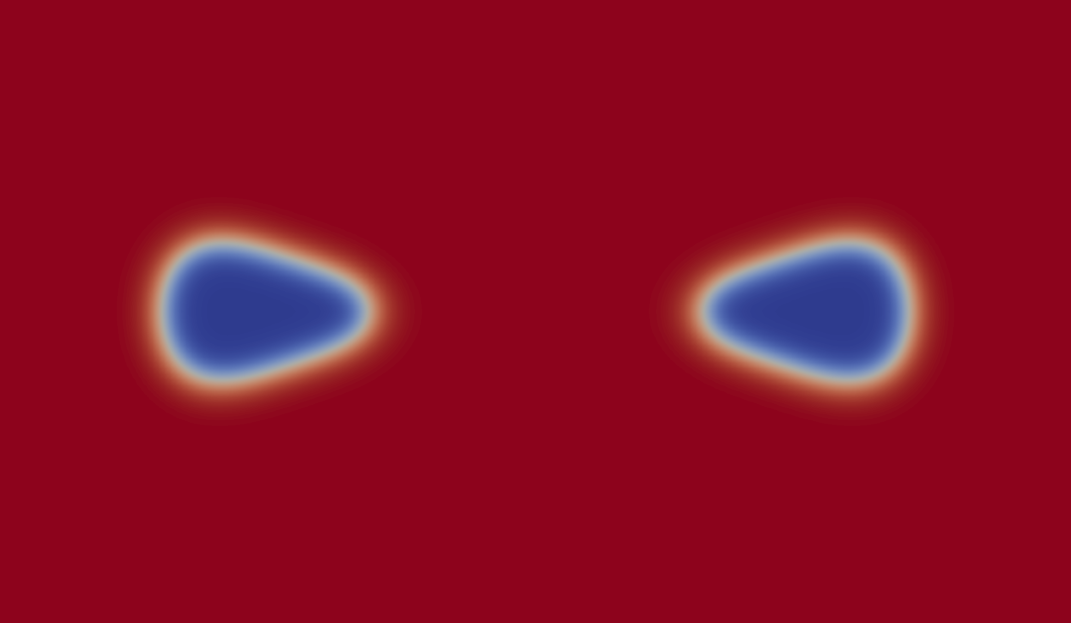
Figure 15: Test 4. The energy minimization method is used. The left graph is the initial condition, and the right graph is the evolution of the solution at $t=0.001$ with $\epsilon=0.01$.

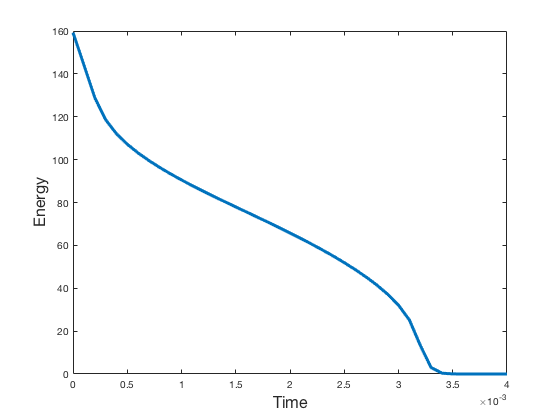
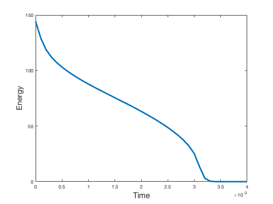
Figure 16: Test 4. The left hand side is the energy of the FIS, and the right hand side is the energy of the energy minimization method with $\epsilon=0.01$.

In Figure 17, the phase field method is used to compute the evolution of the solution, and we find that these two wedges merge, which is consistent with the result of the level set method. The spatial size is $h=0.0033$, the interaction length is $\epsilon=0.0033$, and the time step size is $k=1.11\times 10^{-5}$. In Figure 18, using the same data for Figure 17, the energy minimization method is used to compute the evolution of the solution, and we find that these two wedges also merge, which is consistent with the result of the level set method. Figure 19 indicates the energy change over time for both the phase field method and the energy minimization method. We observe that the energy decreases slowly until around time $7\times 10^{-3}$ for both methods, then it decreases very fast until it reaches 0.

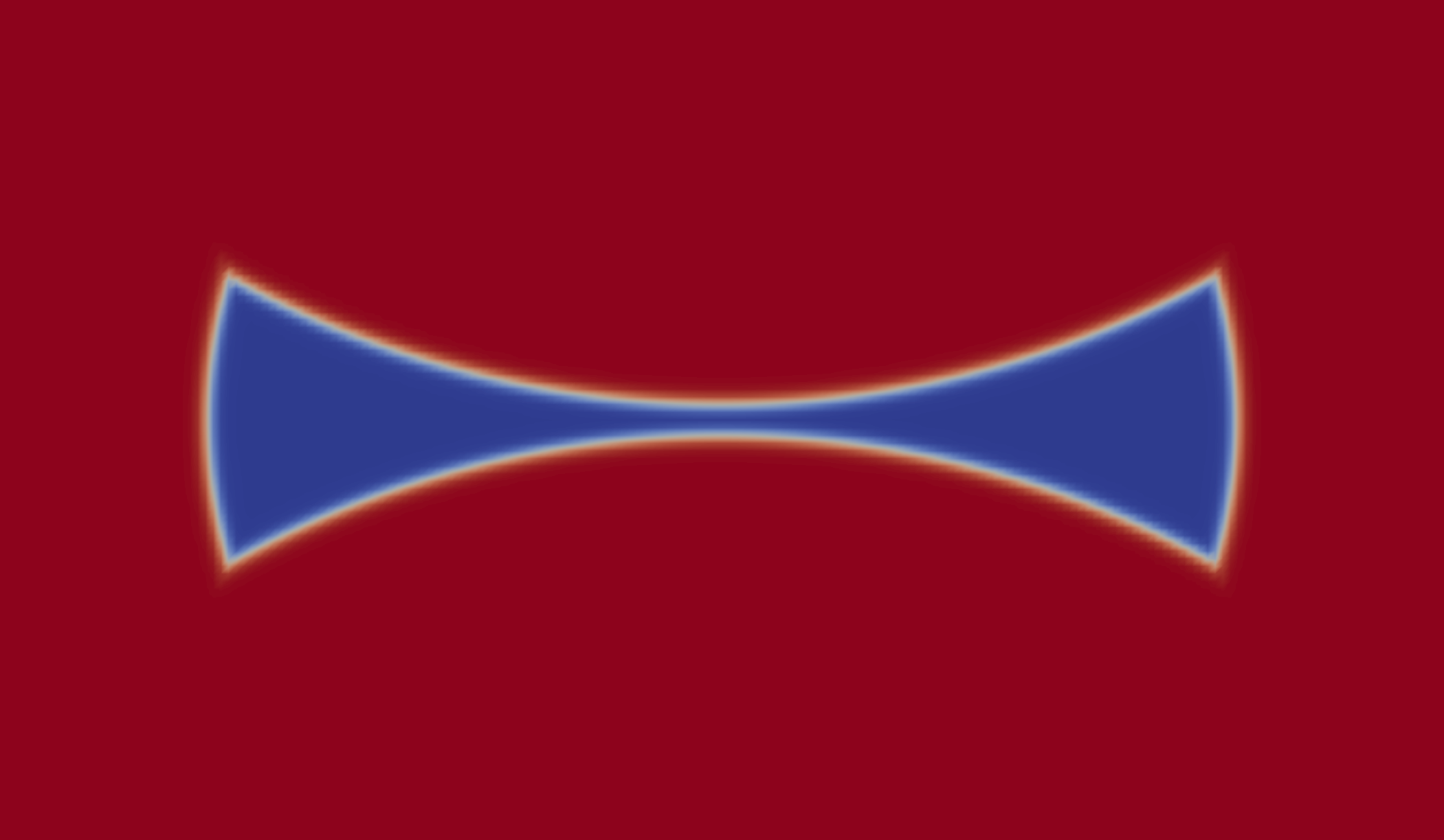
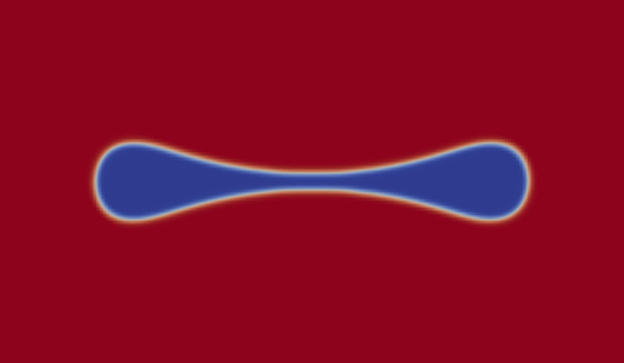
Figure 17: Test 4. The phase field method is used. The left graph is the initial condition, and the right graph is the evolution of the solution at around $t=0.00111$ with $\epsilon=0.0033$.

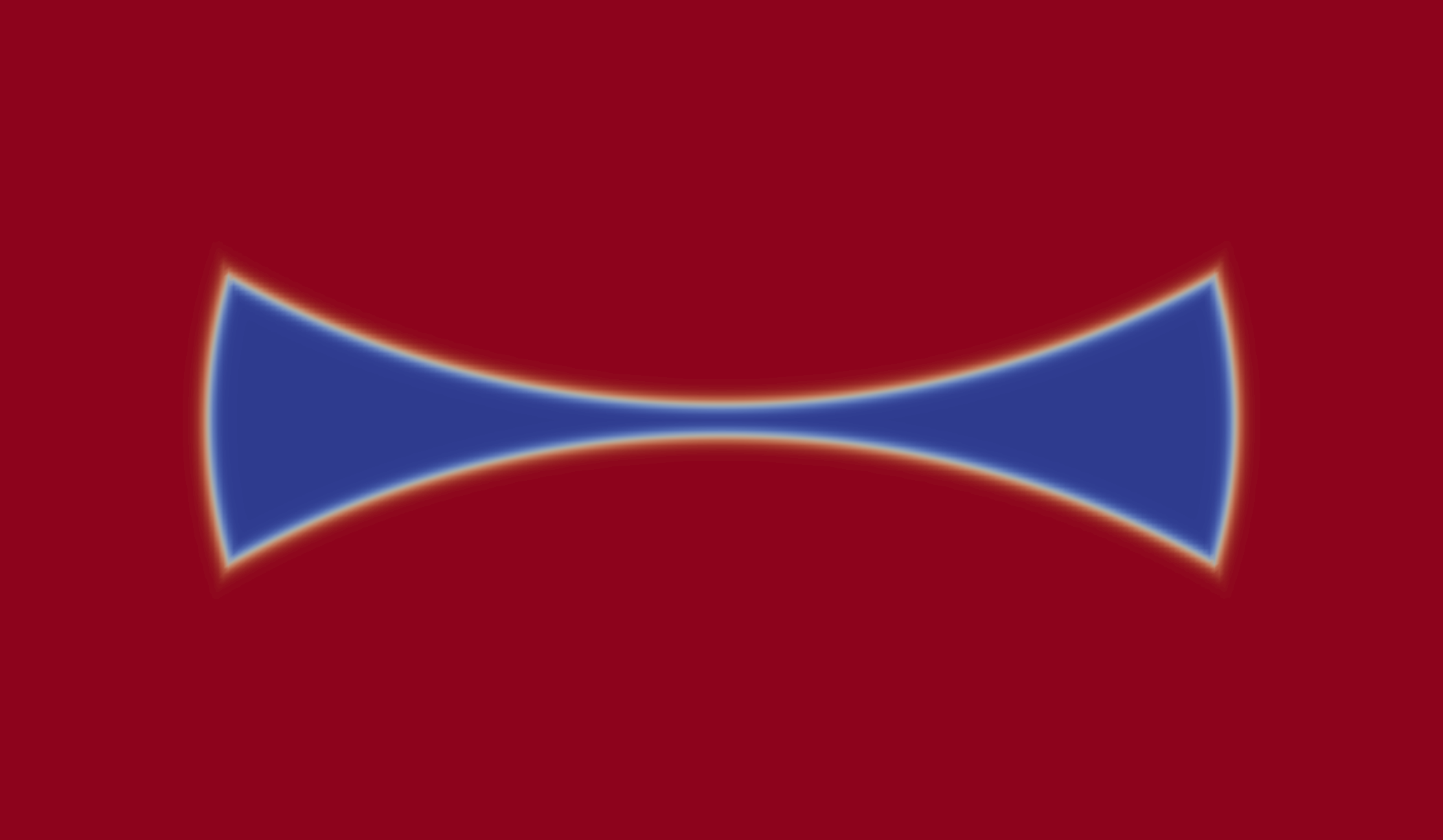
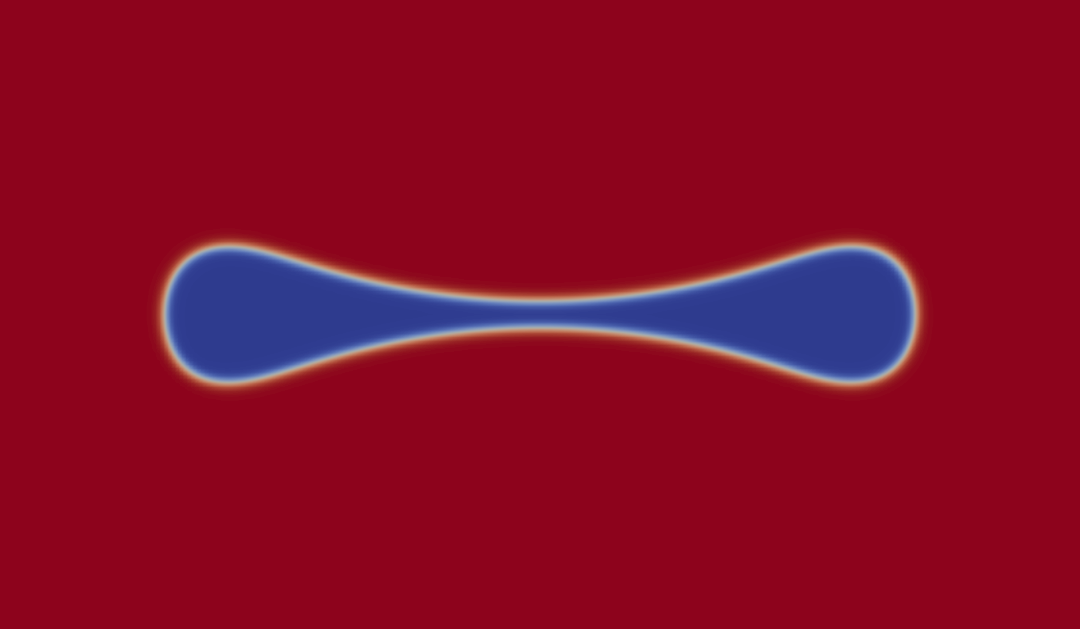
Figure 18: Test 4. The energy minimization method is used. The left graph is the initial condition, and the right graph is the evolution of the solution at around $t=0.00111$ with $\epsilon=0.0033$.

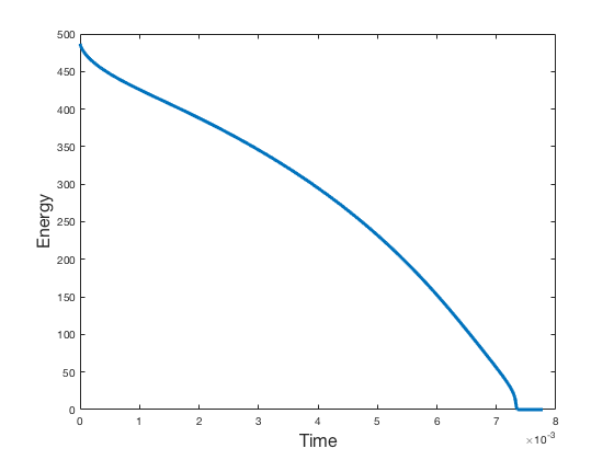
Figure 19: Test 4. The left hand side is the energy of the FIS, and the right hand side is the energy of the energy minimization method with $\epsilon=0.0033$.

3 An Energy Penalized Minimization Algorithm.

In this section, an energy penalized minimization algorithm is proposed to compute the evolution of the mean curvature flow under topological changes. The penalty term has a very similar form as $E_{n}^{\rm AC}(u_{h};u_{h}^{n-1})$, so it is very easy to implement this algorithm. The algorithm is defined by seeking $u_{h}^{n}$ such that

$${u}_{h}^{n}=\underset{u_{h}\in V_{h}}{\mathrm{argmin}}\ \tilde{E}_{n}^{\rm AC}(u_{h};u_{h}^{n-1}).$$ (20)

Here $\tilde{E}_{n}^{\rm AC}(u_{h};u_{h}^{n-1})$ is defined by

$$\tilde{E}_{n}^{\rm AC}(u_{h};u_{h}^{n-1}):=E_{n}^{\rm AC}(u_{h};u_{h}^{n-1})+\delta(\frac{1}{\epsilon^{2}}F(u_{h})-\frac{1}{\epsilon^{2}}F(u_{h}^{n-1})),$$ (21)

where $\delta>0$ is a penalty constant and $E_{n}^{\rm AC}$ is defined in (13).

Next, we will prove the well-posedness and the energy stability of this energy penalized minimization algorithm.

Theorem 3.1

Under the condition that $k\leq\frac{\epsilon^{2}}{1+\delta}$, the solution $u_{h}^{n}$ in (20) exists and is unique.

Proof

By taking the second Fr$\acute{e}$chet derivative of $\tilde{E}_{n}^{\rm AC}(\cdot;u_{h}^{n-1})$, we get for any $v_{h}\in V_{h}$,

$$(\tilde{E}_{n}^{\rm AC})^{\prime\prime}(u_{h};u_{h}^{n-1})(v_{h},v_{h})= \frac{3(1+\delta)}{\epsilon^{2}}\int_{\Omega}u_{h}^{2}v_{h}^{2}dx$$ (22)

$$\qquad+\int_{\Omega}(\frac{1}{k}-\frac{1+\delta}{\epsilon^{2}})v_{h}^{2}dx+\|\nabla v_{h}\|_{L^{2}(\Omega)}^{2}.$$

When $k\leq\frac{\epsilon^{2}}{1+\delta}$ and $v_{h}\neq 0$, $\tilde{E}(\cdot;u_{h}^{n-1})$ is strictly convex on $V_{h}$ since

$$(\tilde{E}_{n}^{\rm AC})^{\prime\prime}(u_{h};u_{h}^{n-1})(v_{h},v_{h})>0.$$

Then $u_{h}^{n}$ is the minimizer of a convex functional, so it exists and is unique.

Instead of using the technique in Theorem 2.1, we use this minimization approach to show the energy stability property of $u_{h}^{n}$.

Theorem 3.2

Under the condition that $k\leq\frac{\epsilon^{2}}{1+\delta}$, the following energy inequality holds

$$\tilde{J}_{\epsilon}^{\rm AC}(u_{h}^{n})+\frac{1}{{\color[rgb]{0,0,0}2k}}\|u_{h}^{n}-u_{h}^{n-1}\|_{L^{2}(\Omega)}^{2}\leq\tilde{J}_{\epsilon}^{\rm AC}(u_{h}^{n-1}),$$

where $\tilde{J}_{\epsilon}^{\rm AC}(v_{h}):=J_{\epsilon}^{\rm AC}(v_{h})+\frac{\delta}{\epsilon^{2}}F(v_{h})$.

Proof

Since $u_{h}^{n}$ is the global minimizer of the convex functional $\tilde{E}_{n}^{\rm AC}$, we have

$$J_{\epsilon}^{\rm AC}(u_{h}^{n})+\frac{1}{{\color[rgb]{0,0,0}2k}}\|u_{h}^{n}-u_{h}^{n-1}\|_{L^{2}(\Omega)}^{2}+\delta(\frac{1}{\epsilon^{2}}F(u_{h}^{n})-\frac{1}{\epsilon^{2}}F(u_{h}^{n-1}))$$

$$= \tilde{E}_{n}^{\rm AC}(u_{h}^{n};u_{h}^{n-1})$$

$$\leq \tilde{E}_{n}^{\rm AC}(u_{h}^{n-1};u_{h}^{n-1})$$

$$= J_{\epsilon}^{\rm AC}(u_{h}^{n-1}).$$

Then the conclusion is obtained directly.

In the following Test 5–Test 7, the energy penalized minimization algorithm is applied to implement the above benchmark problems as well as the problems with random initial conditions.

Test 5. In this test, we compare the evolution of the solution when the initial condition is two circles with a small distance in Test 3 based on the energy penalized minimization algorithm. In Figure 20, the energy penalized minimization algorithm is used to compute the evolution of the solution, and we find that these two circles separate, which is consistent with the result of the level set method. The distance between these two circle is $d=0.02$, the spatial size is $h=0.005$, the interaction length is $\epsilon=0.01$, the penalized term is $\delta=4$, and the time step size is $k=1\times 10^{-4}$.

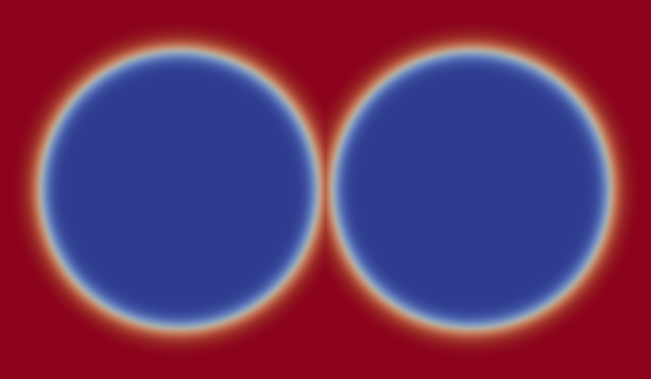
Figure 20: Test 5. The energy penalized minimization algorithm is used. The left graph is the initial condition, and the right graph is the evolution of the solution at $t=0.015$ with $\epsilon=0.01$.

Test 6. In this test, we compare the evolution of the solution under the initial condition in Test 4 based on the energy penalized minimization algorithm. In Figure 21, the energy penalized minimization algorithm with penalized term $\delta$ to be 8 is used to compute the evolution of the solution, and we find that these two wedges merge, which is consistent with the result of the level set method. The spatial size is $h=0.005$, the interaction length is $\epsilon=0.01$, and the time step size is $k=10^{-4}$.

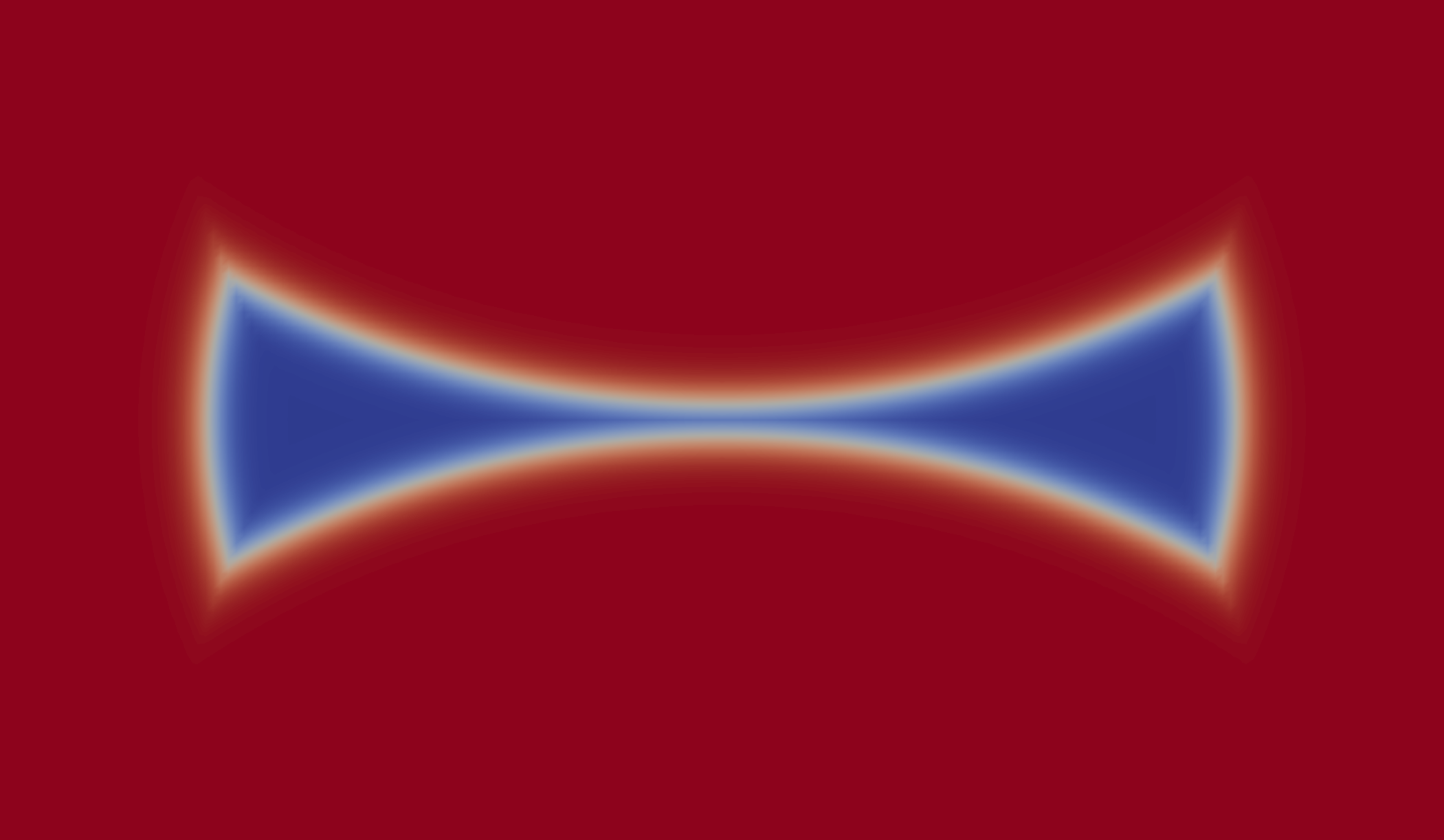
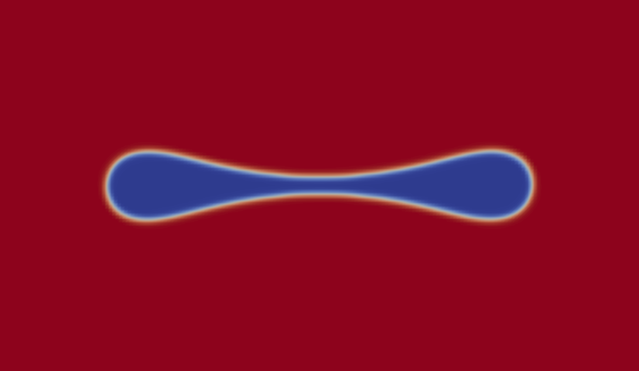
Figure 21: Test 6. The energy penalized minimization algorithm is used. The left graph is the initial condition, and the right graph is the evolution of the solution at $t=0.0015$ with $\epsilon=0.01$.

Test 7. In this test, we compare the evolutions of the solutions when the initial condition is random based on the level set method, the energy minimization method, and the energy penalized minimization algorithm. The domain is $\Omega=[-0.5,0.5]^{2}$. We compute the evolution of the solution after 50 time steps when the initial condition is random, based on the phase field method with time step size $k=10^{-5}$, and then use the resulted solution as the initial condition $u_{0}(x,y)$. We did many tests by choosing different random initial conditions, and we use one example to illustrate the advantages of the proposed energy penalized minimization algorithm in Figures 22–24.

In Figure 22, the level set method is used to compute the evolution of the solution when the random initial condition is used, with the spatial size $h=0.005$ and the time step size $k=6.25\times 10^{-6}$. In Figure 23, the energy minimization method is used. The spatial size is $h=0.005$ and the time step size is $k=5\times 10^{-5}$. We observe that the evolution of the solution computed through the energy minimization is significantly different from the result of the level set method. In Figure 24, the energy penalized minimization algorithm is used. The spatial size is $h=0.005$, the time step size is $k=5\times 10^{-5}$, and the penalized parameter $\delta=8$. We observe that the evolution of the solution computed through the energy penalized minimization algorithm is consistent with the pattern of the level set method.

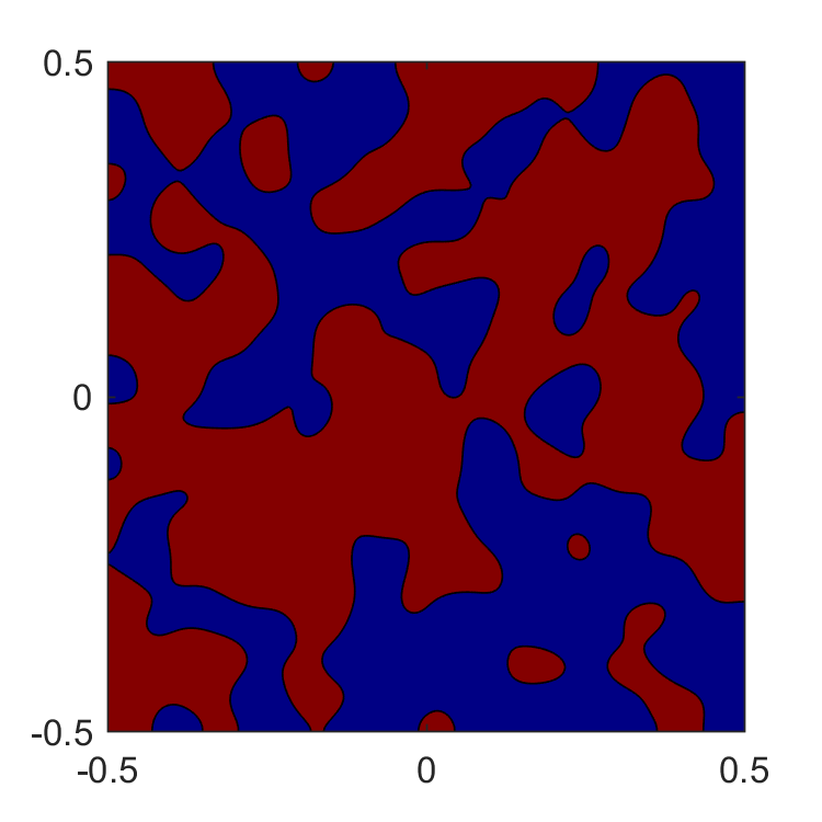
(a) $t=0$

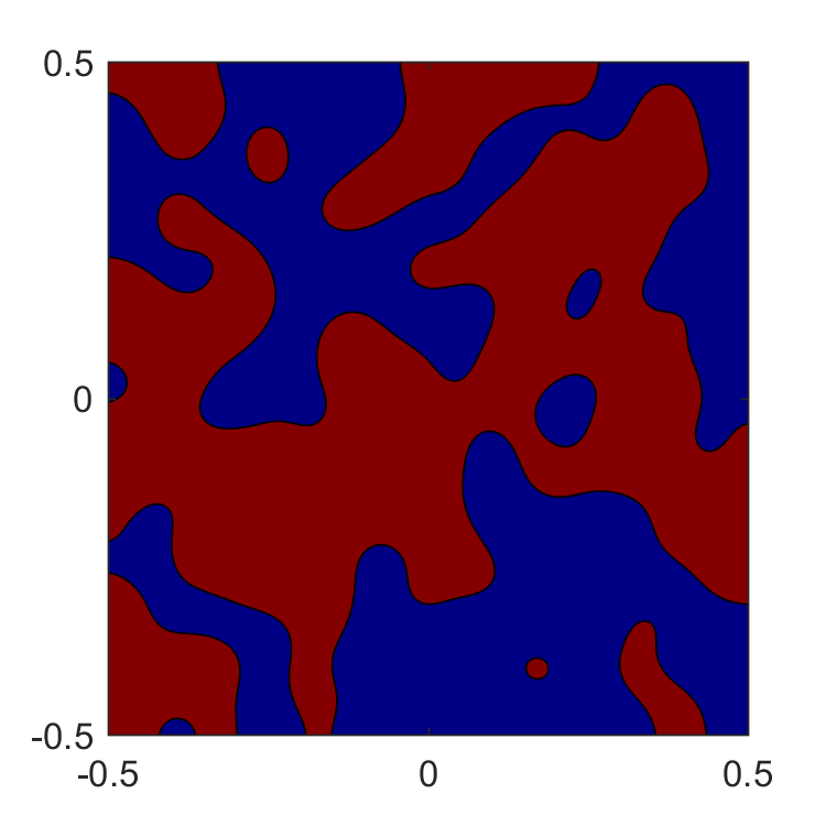
(b) $t=0.0005$

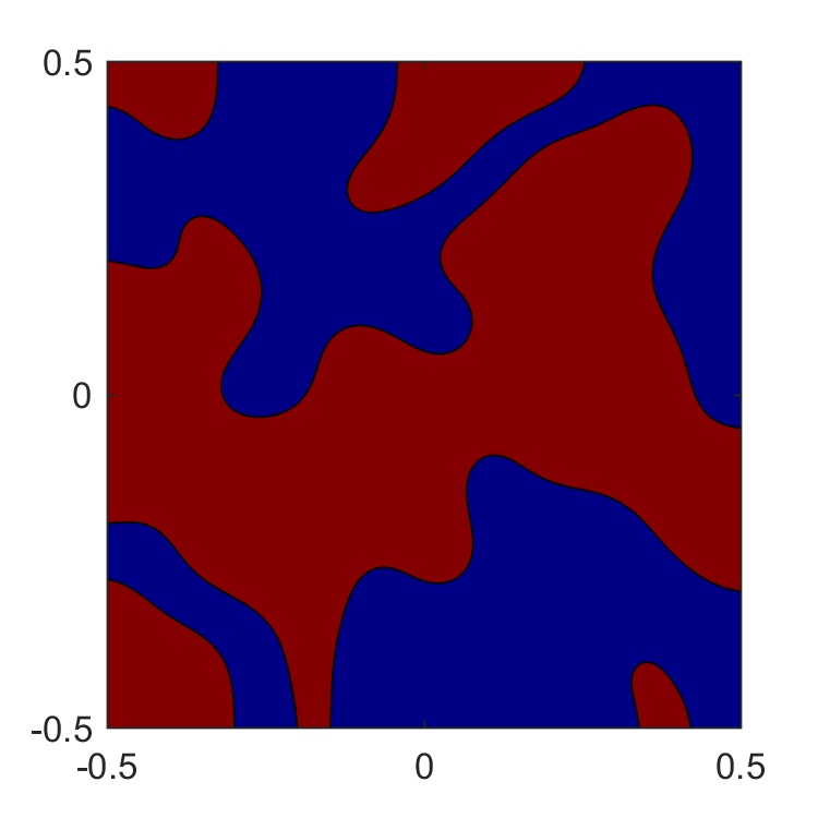
(c) $t=0.002$

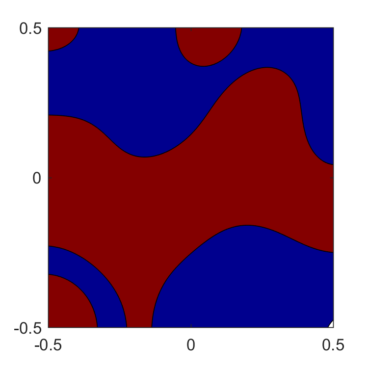
(d) $t=0.01$

Figure 22: Test 7. The level set method is used. The spatial size $h=0.005$ and the time step size $k=6.25\times 10^{-6}$.

(a) $t=0$

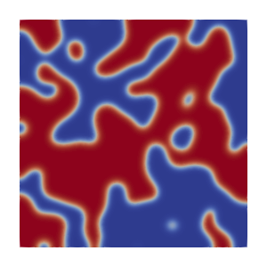
(b) $t=0.0005$

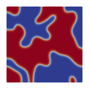
(c) $t=0.002$

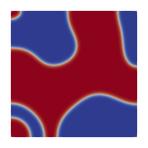
(d) $t=0.01$

Figure 23: Test 7. The energy minimization method is used. The spatial size $h=0.005$ and the time step size $k=5\times 10^{-5}$ with $\epsilon=0.01$.

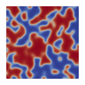
(a) $t=0$

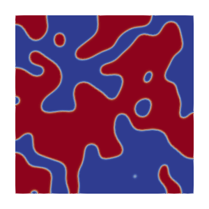
(b) $t=0.0005$

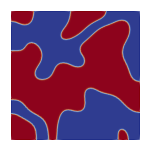
(c) $t=0.002$

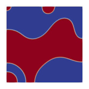
(d) $t=0.01$

Figure 24: Test 7. The energy penalized minimization algorithm is used. The spatial size $h=0.005$ and the time step size $k=5\times 10^{-5}$ with $\epsilon=0.01$.

4 A Multilevel Minimization Algorithm.

The coarse to fine multilevel minimization algorithm is defined by seeking, at each time step iteration, ${\color[rgb]{0,0,0}{u}_{h_{m}}^{n}}$ such that

$${u}_{{\color[rgb]{0,0,0}h_{1}}}^{n-1} =\underset{u_{{\color[rgb]{0,0,0}h_{1}}}\in V_{{\color[rgb]{0,0,0}h_{1}}}}{\mathrm{argmin}}\ E^{AC}_{n,{\color[rgb]{0,0,0}\epsilon_{1}}}(u_{{\color[rgb]{0,0,0}h_{1}}};u^{n-1}_{h_{m}}),$$

$${u}_{{\color[rgb]{0,0,0}h_{2}}}^{n-1} =\underset{u_{{\color[rgb]{0,0,0}h_{1}}}\in V_{{\color[rgb]{0,0,0}h_{2}}}}{\mathrm{argmin}}\ E^{AC}_{n,{\color[rgb]{0,0,0}\epsilon_{2}}}(u_{{\color[rgb]{0,0,0}h_{2}}};u^{n-1}_{h_{m}}),$$

$$\vdots$$

$${\color[rgb]{0,0,0}{u}_{h_{m}}^{n}} =\underset{u_{{\color[rgb]{0,0,0}h_{m}}}\in V_{{\color[rgb]{0,0,0}h_{m}}}}{\mathrm{argmin}}\ E^{AC}_{n,{\color[rgb]{0,0,0}\epsilon_{m}}}(u_{{\color[rgb]{0,0,0}h_{m}}};u^{n-1}_{h_{m}}),$$

where $h_{1}>h_{2}>\cdots>h_{m}$, $\epsilon_{1}>\epsilon_{2}>\cdots>\epsilon_{m}$, $V_{h_{i}}$ is the discrete space associated to $h_{i}$, and $E^{AC}_{n,{\color[rgb]{0,0,0}\epsilon_{i}}}$ is the energy defined in 13 using $\epsilon_{i}$ instead of $\epsilon$. This means that for the first few steps , when $\epsilon_{i}$ and $h_{i}$ are large, our energy minimization should converge quickly. Then, when $\epsilon_{i}$ and $h_{i}$ are smaller, the minimization algorithm is able to converge due to the fact that the initial guess which is the solution from the previous mesh is close enough to the physical solution. Note that this method requires to project the solution obtained from the previous step to the new mesh; as for the minimization algorithm we use the limited memory BFGS method, see nocedal1980 .

One of the issues of using the traditional energy minimization method when the energy is not convex is that the solution is dependent on the initial guess. The method we propose to solve this issue is, at a fix time step, first minimizing the energy with a larger $\epsilon$ in order to start with a convex energy functional, and then decreasing $\epsilon$ in the next steps. Regarding the fully implicit scheme for the Allen-Cahn equation, equation (8), we recall the following two important conditions we need:

1. Convexity condition: ${\color[rgb]{0,0,0}k}\leq\epsilon^{2}$

2. Mesh size relation to $\epsilon$: $h^{-1}=\mathcal{O}(\epsilon^{-1})$

In the following Test 8 and Test 9, the traditional energy minimization algorithm and the coarse to fine multilevel minimization algorithm are compared for the cases when there are no topological changes (Test 8) and there are topological changes (Test 9).

Test 8. To test this method we pick the following: $h=10^{-3}$, $\epsilon=0.005$, and

$$u_{0}(x,y)=\tanh\bigl{(}\frac{d_{0}(x,y)}{\sqrt{2}\epsilon}\bigr{)}.$$ (23)

For our initial guess we chose $u=1-u_{0}(x,y)$. We remark that when $\epsilon$ is large, by following the condition $h=\mathcal{O}(\epsilon)$, we can pick a larger mesh size. This leads up to the following multilevel algorithms:

$h=0.12$, $\epsilon=0.1$	$\longrightarrow$	$h=0.07$, $\epsilon=0.076$	$\longrightarrow$	$h=0.035$, $\epsilon=0.028$	$\cdots$

We chose 5 different meshes with the following $h$ and $\epsilon$ in Table 1.

Mesh	$h$	$\epsilon$
1	0.12	0.1
2	0.07	0.076
3	0.035	0.28
4	0.018	0.29
5	0.009	0.005

Table 1: Meshes on different levels.

Then, after doing one step in time we compare the multilevel solution and the solution computed by using the fine mesh only. Figure 25 (right) displays the cross-sectional solutions at $y=0$ at $t=0.001$. We know, from xu2019stability , that the correct solution is a circle of depth $-1$, see Figure 25 (left). Figure 25 (right) shows that the solution computed using the multilevel algorithm is the correct one. Notice the energy functional is convex for the coarse meshes of the multilevel minimization algorithm, but it is not convex for the fine meshes. We observe that the proposed multilevel minimization algorithm is useful to handle the issue of the initial guess when the energy functional is not convex.

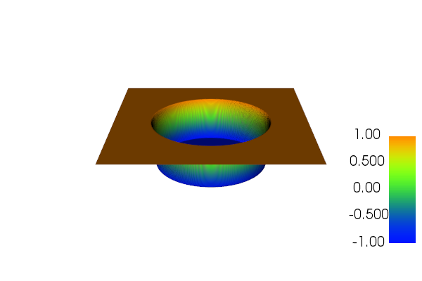
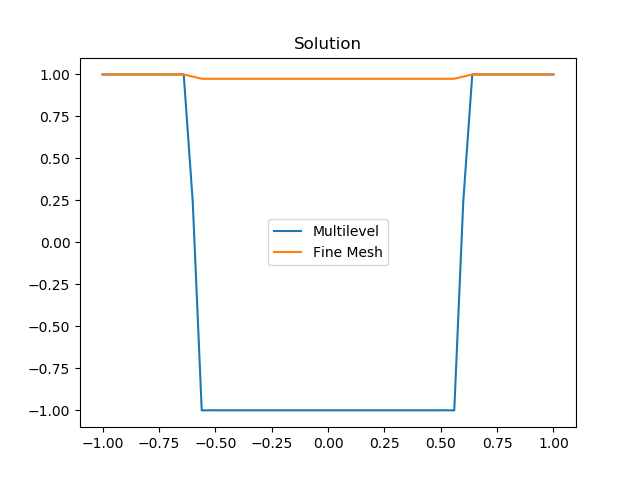
Figure 25: Test 8. Left: Initial value of $u$ for the Allen-Cahn equation. Right: Cross-sectional solutions to the Allen-Cahn equation at $y=0$ and $t=0.001$ of the regular and multilevel methods.

Test 9. In this test, we compare the evolutions of the solutions based on the multilevel minimization algorithm and the traditional energy minimization algorithm (14) under the initial condition of two circles with a small distance. The distance between two circles is $d=0.02$, the spatial size is $h=0.002$, the time step is $k=1\times 10^{-4}$, and the interaction length is $\epsilon=0.002$. The initial guess we choose is: $u=1-u_{0}(x,y).$

Figure 26 shows the evolution of the solution based on the traditional energy minimization algorithm. We observe that two circles become two round-shape shadows at $t=0.0001$, which is not correct.

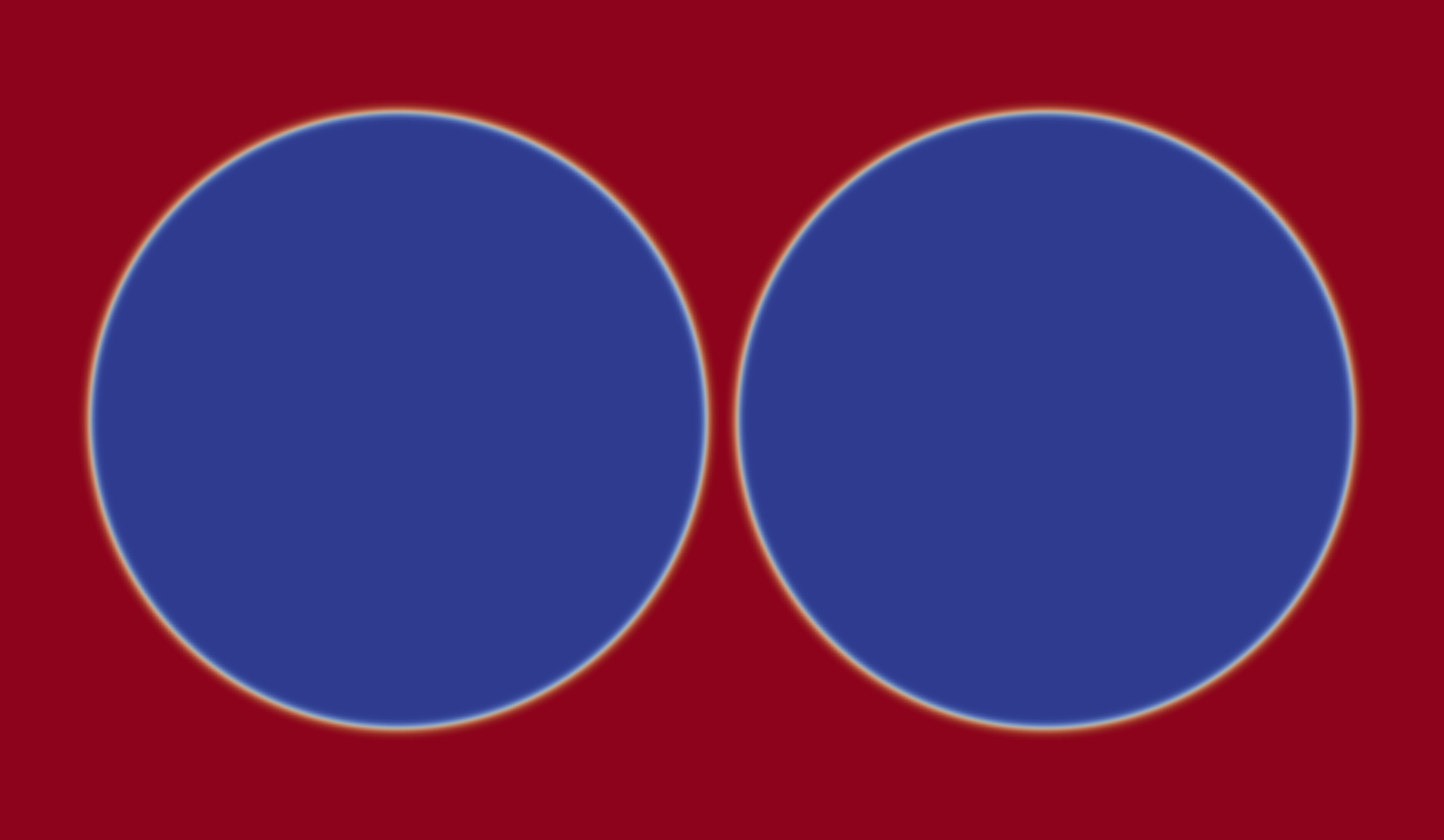
Figure 26: Test 9. The traditional energy minimization algorithm is used. The graph on the left is the initial condition, and the graph on the right is the evolution of the solution at $t=0.0001$ with $\epsilon=0.002$.

Figure 27 shows the evolution of the solution based on the coarse to fine multilevel minimization algorithm. We observe that these two circles separate, which is consistent with the level set method. The distance between these two circles is $d=0.02$ and the time step size is $k=1\times 10^{-4}$. Specifically, for the multilevel method, we pick $\epsilon$ and the spatial size $h$ in Table 2 below:

Mesh	$h$	$\epsilon$
1	0.002	0.0047
2	0.001	0.00335
3	0.0005	0.002

Table 2: Meshes on different levels

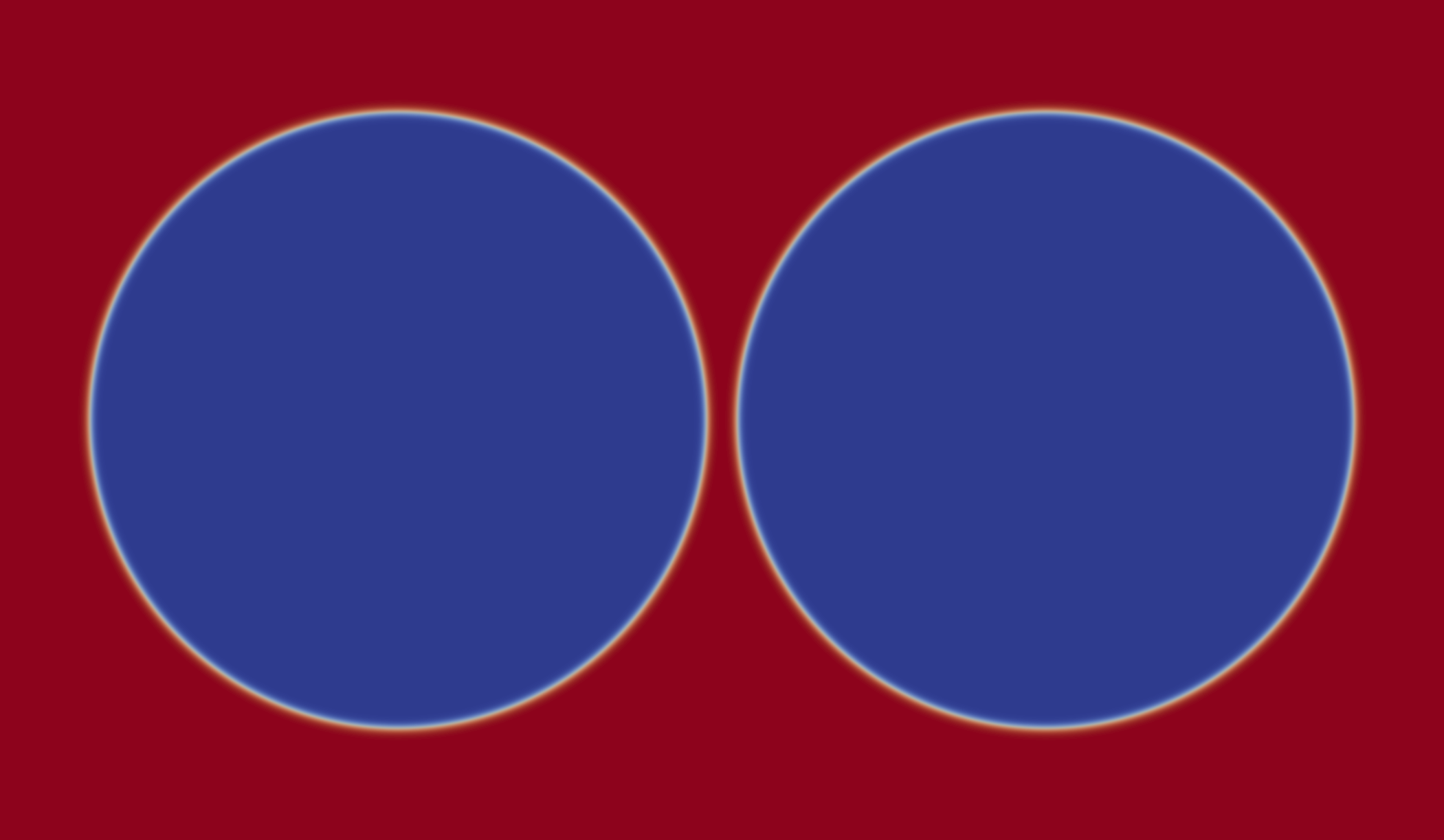
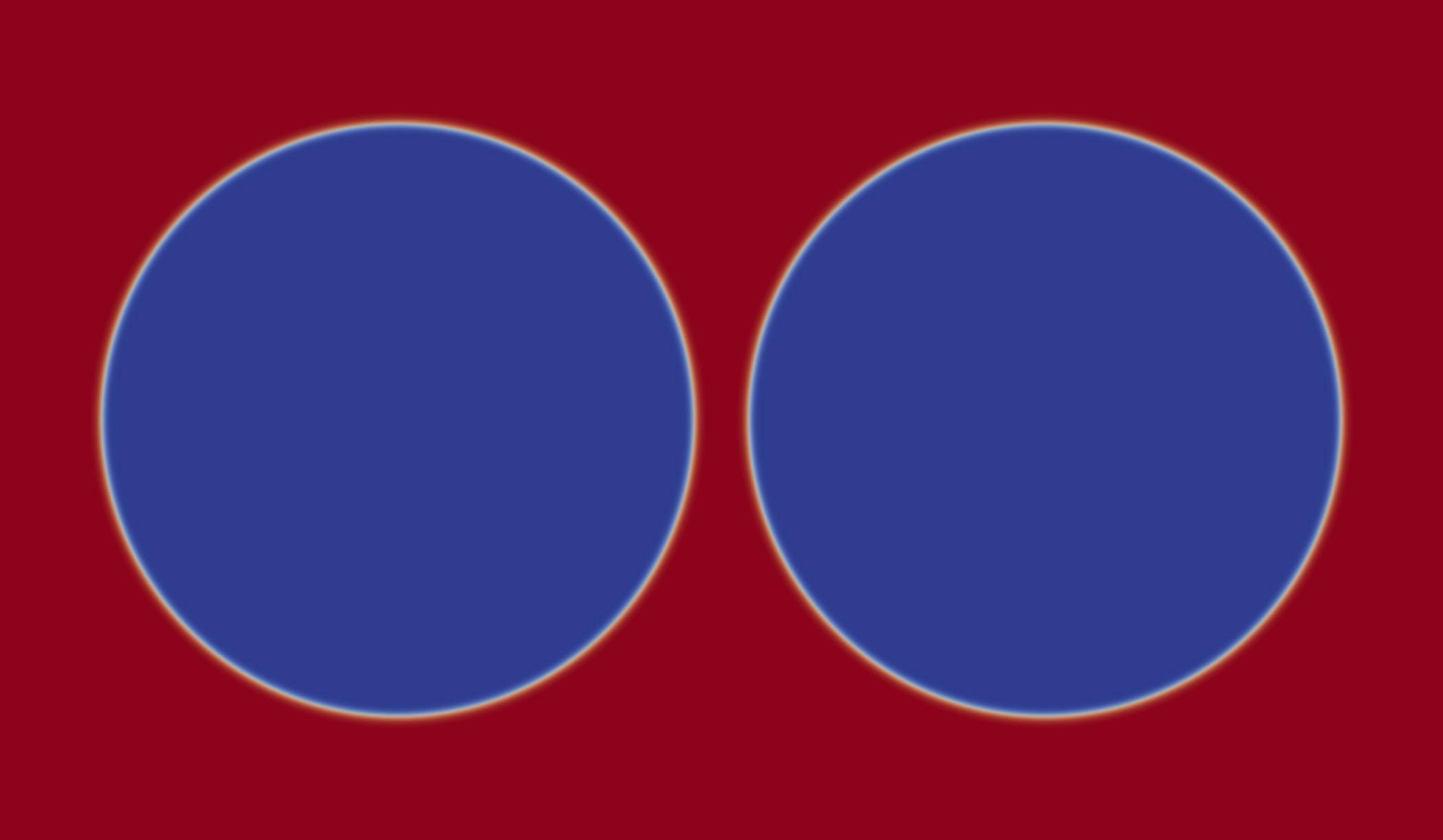
Figure 27: Test 9. The multilevel minimization algorithm algorithm is used. The graph on the left is the initial condition, and the graph on the right is the evolution of the solution at $t=0.0015$.

This test indicates that the traditional energy minimization algorithm may not be able to carry out the evolution of the solution correctly when the initial guess is not good and when there are topological changes. But the multilevel minimization algorithm may overcome the problem and produce the correct results.

5 Conclusion.

In this paper, we propose some algorithms to compute the mean curvature flow under topological changes based on the phase field methodology, and the objective is to validate these algorithms for the random initial conditions. To achieve this objective, some benchmark problems are constructed first, and it is shown that the evolutions of the solutions are very sensitive to the interaction length $\epsilon$ when topological changes happen. The energy penalized minimization algorithm is proposed to accurately solve these benchmark problems and the problems with random initial conditions in Section 3. Besides, the issue of traditional energy minimization algorithm arises from the existence of multiple minimum points due to the non-convexity property of the energy functional. This issue can be removed by using a multilevel algorithm and starting from a convex problem in Section 4. With the multilevel algorithm, the solution converges to the global minimum. Furthermore, in Test 9, we show that when topological changes happen, the traditional energy minimization algorithm also encounters the convexity problem and fails to produce a correct solution. Fortunately, the multilevel algorithm is not only able to remove the convexity problem, but also able to carry out the evolution of the solution accurately.

Lastly, we are also thinking about how to improve even further our energy minimization algorithms. We could think about using the multilevel methods inside the nonlinear solver. Instead of doing all the minimization steps on coarse meshes, we could first do some steps on the coarser meshes and then project the solution on the finer meshes. This could in theory reduce the time needed by our nonlinear solver.

References

- (1) Bousquet A, Li Y, Wang G (2019) Some algorithms for the mean curvature flow under topological changes, arXiv preprint arXiv:1908.09690.
- (2) Barrett J, Garcke H, Nürnberg R (2007) A parametric finite element method for fourth order geometric evolution equations, J. Comput. Phys. 222: pp. 441–467.
- (3) Bartels S, Müller R (2011) Quasi-optimal and robust a posteriori error estimates in for the approximation of Allen-Cahn equations past singularities, Math. Comp. 80: pp. 761–780.
- (4) Bartels S, Müller R, Ortner C (2011) Robust a priori and a posteriori error analysis for the approximation of Allen-Cahn and Ginzburg-Landau equations past topological changes, SIAM J. Numer. Anal. 49: pp. 110–134.
- (5) Bartels S (2010) A lower bound for the spectrum of the linearized Allen-Cahn operator near a singularity.
- (6) Chen Y, Giga Y, Goto S, others (1991), Uniqueness and existence of viscosity solutions of generalized mean curvature flow equations, J. Differential Geom. 33: pp. 749–786.
- (7) Church M, Guo Z, Jimack P, Madzvamuse A, Promislow K, Wetton B, Wise S, Yang F (2019) High accuracy benchmark problems for Allen-Cahn and Cahn-Hilliard dynamics, Commun. Comput. Phys..
- (8) Cesaroni A, Dipierro S, Novaga M, Valdinoci E (2018) Fattening and nonfattening phenomena for planar nonlocal curvature flows, Math. Ann.: pp. 1–50.
- (9) Deckelnick K, Dziuk G (2003) Numerical approximation of mean curvature flow of graphs and level sets, Mathematical aspects of evolving interfaces, pp. 53–87.
- (10) Du Q, Liu C, Wang X (2005) Retrieving topological information for phase field models, SIAM J. Appl. Math. 65: pp. 1913–1932.
- (11) Elliott C, Fritz H (2017) On approximations of the curve shortening flow and of the mean curvature flow based on the DeTurck trick, IMA J. Numer. Anal. 37: pp. 543–603.
- (12) Evans L, Soner H, Souganidis P (1992) Phase transitions and generalized motion by mean curvature, Comm. Pure Appl. Math. 45: pp. 1097–1123.
- (13) Evans L, Spruck J (1991) Motion of level sets by mean curvature I, J. Differential Geom. 33: pp. 635–681.
- (14) Feng X, Prohl A (2003) Numerical analysis of the Allen-Cahn equation and approximation for mean curvature flows, Numer. Math. 94: pp. 33–65.
- (15) Feng X, Wu H (2005) A posteriori error estimates and an adaptive finite element algorithm for the Allen-Cahn equation and the mean curvature flow, J. Sci. Comput. 24: pp. 121–146.
- (16) Feng X, Li Y, Prohl A (2014) Finite element approximations of the stochastic mean curvature flow of planar curves of graphs, Stochastic Partial Differential Equations: Analysis and Computations 2: pp. 54–83.
- (17) Feng X, Li Y (2014) Analysis of symmetric interior penalty discontinuous Galerkin methods for the Allen-Cahn equation and the mean curvature flow, IMA J. Numer. Anal. 35: pp. 1622–1651.
- (18) Feng X, Li Y, Xing Y (2016) Analysis of mixed interior penalty discontinuous Galerkin methods for the Cahn-Hilliard equation and the Hele-Shaw flow, SIAM J. Numer. Anal. 54: pp. 825–847.
- (19) Feng X, Li Y, Zhang Y (2017) Finite element methods for the stochastic Allen-Cahn equation with gradient-type multiplicative noise, SIAM J. Numer. Anal. 55: pp. 194–216.
- (20) Hirt C, Nichols B (1981) Volume of fluid (VOF) method for the dynamics of free boundaries, J. Comput. Phys. 39: pp. 201–225.
- (21) Kessler D, Nochetto R, Schmidt A (2004) A posteriori error control for the Allen-Cahn problem: circumventing Gronwall’s inequality, ESAIM Math. Model. Numer. Anal. 38: pp. 129–142.
- (22) Kovács B, Li B, Lubich C (2018) A convergent evolving finite element algorithm for mean curvature flow of closed surfaces, arXiv preprint arXiv:1805.06667.
- (23) Li Y (2015) Numerical methods for deterministic and stochastic phase field models of phase transition and related geometric flows, Ph.D. thesis, The University of Tennessee.
- (24) Li Y (2019) Error analysis of a fully discrete Morley finite element approximation for the Cahn-Hilliard equation, J. Sci. Comput. 78: 1862-1892.
- (25) Feng X, Li Y, Zhang Y (2018) Strong convergence of a fully discrete finite element method for a class of semilinear stochastic partial differential equations with multiplicative noise, Comput. Math..
- (26) Leveque R, Li Z (1994) The immersed interface method for elliptic equations with discontinuous coefficients and singular sources, SIAM J. Numer. Anal. 31: pp. 1019–1044.
- (27) Majee A, Prohl A (2018) Optimal Strong rates of convergence for a space-time discretization of the stochastic Allen–Cahn equation with multiplicative noise, Comput. Methods Appl. Math. 18: pp. 297–311.
- (28) Nocedal J. (1980) Updating quasi-Newton matrices with limited storage. Math. Comp. 35, no. 151, pp. 773–782.
- (29) Osher S and Sethian J (1998) Fronts propagating with curvature-dependent speed: algorithms based on Hamilton-Jacobi formulations, J. Comput. Phys. 79: pp. 12–49.
- (30) Peskin C (2002) The immersed boundary method, Acta Numer. 11: pp. 479–517.
- (31) Rayleigh L (1892) On the theory of surface forces. II. Compressible fluids, The London, Edinburgh, and Dublin Philosophical Magazine and Journal of Science 33: pp. 209–220.
- (32) Shen J, Tang T, Wang L, (2011) Spectral methods: algorithms, analysis and applications, Springer Science & Business Media 41.
- (33) Ilmanen T, others (1993) Convergence of the Allen-Cahn equation to Brakke’s motion by mean curvature, J. Differential Geom 38: pp. 417–461.
- (34) Unverdi S, Tryggvason G (1992) A front-tracking method for viscous, incompressible, multi-fluid flows, J. Comput. Phys. 100: pp. 25–37.
- (35) Walkington N (1996) Algorithms for computing motion by mean curvature, SIAM J. Numer. Anal. 33: pp. 2215–2238.
- (36) Wu S, Li Y (2019) Analysis of the Morley element for the Cahn-Hilliard equation and the Hele-Shaw flow, ESAIM Math. Model. Numer. Anal., accepted.
- (37) Xu J, Li Y, Wu S, Bousquet A (2019) On the stability and accuracy of partially and fully implicit schemes for phase field modeling, Comput. Methods Appl. Mech. Engrg. 345: pp. 826-853.
- (38) Zhang J, Du Q (2009) Numerical studies of discrete approximations to the Allen–Cahn equation in the sharp interface limit, SIAM J. Numer. Anal. 31: pp. 3042–3063.