Statistical sensitivity estimates for oscillating electric dipole moment measurements in storage rings

Abstract

In this paper analytical expressions are derived to describe the spin motion of a particle in magnetic and electric fields in the presence of an axion field causing an oscillating electric dipole moment (EDM). These equations are used to estimate statistical sensitivities for axion searches at storage rings.

The estimates obtained from the analytic expressions are compared to numerical estimates from simulations in reference Chang:2019poy . A good agreement is found.

1 Introduction and motivation

Axions and axion like particles (ALPs) are candidates for dark matter. There is thus a huge experimental effort for the search of these kind of particles. For a detailed review, we refer the reader to references Graham:2015ouw ; Irastorza:2018dyq . Axions and ALPs can interact with ordinary matter in various ways. Reference Graham:2013gfa identifies three terms:

$$\frac{a}{f_{0}}\,F_{\mu\nu}\tilde{F}_{\mu\nu},\quad\frac{a}{f_{a}}\,G_{\mu\nu}\tilde{G}_{\mu\nu},\quad\frac{\partial_{\mu}a}{f_{a}}\bar{\Psi}_{f}\gamma^{\mu}\gamma_{5}\Psi$$ (1)

describing the coupling to photons, gluons and to the spin of fermions, respectively. The vast majority of experiments makes use of the first term (e.g. Cavity experiments (ADMX), helioscopes (CAST), light-through-wall experiments (ALPS)). In addition, astrophysical observations also provide sensitive limits to the axion-photon coupling. In general, it is rather difficult for these experiments to reach masses below $10^{-6}\,$\mathrm{e}\mathrm{V}$$, one reason being that the axion wave length becomes too large. Furthermore, these experiments are measuring rates proportional to at least a small amplitude squared.

For the second (and third) term in the list (1) this is different. It turns out that the second term has the same structure as the QCD-$\theta$ term which is also responsible for an electric dipole moment (EDM) of nucleons. The axion field gives rise to an effective time-dependent $\theta$-term and oscillates at a frequency proportional to the mass of the axion $m_{a}$. This gives rise to an oscillating EDM. New opportunities to search for axions/ALPs with much higher sensitivity arise, because the signal is proportional to an amplitude $A$ and not to its square. To date, NMR based methods are being used to look at oscillating EDMs Budker:2013hfa .

Another possibility is to search for axions/ALPs in storage rings. Storage ring experiments have been proposed to search for electric dipole moments of charge particles Anastassopoulos:2015ura ; Abusaif:2019gry . These experiments allow also, with small modifications, to search for oscillating EDMs. This possibility is discussed in this paper. Section 2 explains the principle of the experiment, how the (oscillating) EDM alters the spin motion in electromagnetic fields and leads to a polarization observable. In section 3 statistical sensitivities for oscillating EDMs based on these polarization are presented.

2 Spin motion in storage rings

The spin motion relative to the momentum vector in electric and magnetic fields is governed by the Thomas-BMT equation  Bargmann:1959gz ; Nelson:1959zz ; Fukuyama:2013ioa :

$$\frac{d\vec{S}}{dt} = (\vec{\Omega}_{\mathrm{MDM}}+\vec{\Omega}_{\mathrm{EDM}})\times\vec{S},$$ (2)

$$\vec{\Omega}_{\mathrm{MDM}} = -\frac{q}{m}~{}\left[G\vec{B}-\left(G-\frac{1}{\gamma^{2}-1}\right)\frac{\vec{\beta}\times\vec{E}}{c}\right],$$ (3)

$$\vec{\Omega}_{\mathrm{EDM}} = -\frac{\eta q}{2mc}\left[\vec{E}+c\vec{\beta}\times\vec{B}\right].$$ (4)

$\vec{S}$ in this equation denotes the spin vector in the particle rest frame, $t$ the time in the laboratory system, $\beta$ and $\gamma$ the relativistic Lorentz factors, and $\vec{B}$ and $\vec{E}$ the magnetic and electric fields in the laboratory system, respectively. The magnetic dipole moment $\vec{\mu}$ and electric dipole moment $\vec{d}$ both pointing in the direction of the particle’s spin $\vec{S}$ are related to the dimensionless quantities $G$ (magnetic anomaly) and $\eta$ in equation 2:

$$\vec{\mu}=g\frac{q\hbar}{2m}\vec{S}=(1+G)\frac{q\hbar}{m}\vec{S}\,\quad\mbox{and}\quad\vec{d}=\eta\frac{q\hbar}{2mc}\vec{S}\,.$$ (5)

We assume a vertical magnetic field and a radial electric field, constant in time, forcing the particle on a circular orbit. The three vectors $\vec{B}$, $\vec{E}$ and $\vec{v}=\vec{\beta}c$ are thus mutually orthogonal, as indicated in figure 1. In this case

$$\vec{\Omega}_{\mathrm{MDM}}=\left(\begin{array}[]{c}0\\ \Omega_{\mathrm{MDM}}\\ 0\\ \end{array}\right)\quad\mbox{and}\quad\vec{\Omega}_{\mathrm{EDM}}=\left(\begin{array}[]{c}\eta\tilde{\Omega}_{\mathrm{EDM}}\\ 0\\ 0\\ \end{array}\right)$$ (6)

with $\Omega_{\mathrm{MDM}}=-\frac{q}{m}(GB+\left(G-\frac{1}{\gamma^{2}-1}\right)\frac{\beta E}{c})$ and $\tilde{\Omega}_{\mathrm{EDM}}=-\frac{q}{2mc}(E+c\beta B)$, $B=|\vec{B}|$ and $E=|\vec{E}|$. The coordinate system is chosen such that the first component points in radial direction, the second in vertical and the third in longitudinal direction. Note that $\vec{\beta}\times\vec{E}$ is anti-parallel to $\vec{B}$. This explains the $+$ sign in front of $\left(G-\frac{1}{\gamma^{2}-1}\right)$ in the definition of $\Omega_{\mathrm{MDM}}$ instead of a $-$ sign in equation 3.

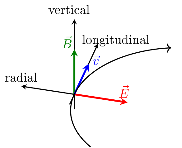
Figure 1: Illustration of the coordinate system used.

For the following discussion it is more convenient to write equation 2 in matrix form:

$$\frac{d\vec{S}}{dt}=(A_{\mathrm{MDM}}+A_{\mathrm{EDM}})\vec{S}$$ (7)

with (to simplify the notation we use $\Omega_{\mathrm{EDM}}$ instead of $\tilde{\Omega}_{\mathrm{EDM}}$ from now on)

$$A_{\mathrm{MDM}}=\left(\begin{array}[]{ccc}0&0&\Omega_{\mathrm{MDM}}\\ 0&0&0\\ -\Omega_{\mathrm{MDM}}&0&0\\ \end{array}\right)\quad\mbox{and}\quad A_{\mathrm{EDM}}=\eta\left(\begin{array}[]{ccc}0&0&0\\ 0&0&\Omega_{\mathrm{EDM}}\\ 0&-\Omega_{\mathrm{EDM}}&0\\ \end{array}\right)\,.$$ (8)

In the following we assume that the EDM can have a constant term and a time varying component, thus $\eta=\eta_{0}+\eta_{1}\cos(\omega_{a}t+\varphi_{a})$ as suggested in  Graham:2013gfa ; Graham:2011qk . The oscillating term is caused by an axion of mass given by the relation $\omega_{a}=m_{a}c^{2}/\hbar$. Assuming $\eta_{0},\eta_{1}\ll G$, $A_{\mathrm{EDM}}$ in equation 7 can be treated as an perturbation.

The solution to first order in $\eta_{0}$ and $\eta_{1}$ for arbitrary initial condition of the spin is given in Appendix A. The best sensitivity to $\eta_{0}$ and $\eta_{1}$ is obtained by observing a build-up of a vertical polarization of a beam initially polarized in the horizontal plane. Thus we are interested in the behavior of the vertical spin component $S_{v}(t)$ in the case where the spin points for example initially in the longitudinal direction ($\vec{S}(0)=(0,0,1)^{T}$). Using equation 37 in Appendix A one finds:

$$S_{v}(t) = \eta_{0}\Omega_{\mathrm{EDM}}\frac{\sin(\Omega_{\mathrm{MDM}}t)}{\Omega_{\mathrm{MDM}}}+\eta_{1}\,\frac{\Omega_{\mathrm{EDM}}}{2(\omega_{a}-\Omega_{\mathrm{MDM}})(\Omega_{\mathrm{MDM}}+\omega_{a})}$$ (9)

$$\Big{[}-2\omega_{a}\sin(\varphi_{a})$$

$$+(\omega_{a}+\Omega_{\mathrm{MDM}})\sin((\omega_{a}-\Omega_{\mathrm{MDM}})t+\varphi_{a})$$

$$+(\omega_{a}-\Omega_{\mathrm{MDM}})\sin((\Omega_{\mathrm{MDM}}+\omega_{a})t+\varphi_{a})\Big{]}\,.$$

We are interested in the behavior close to the resonance condition $\Omega_{\mathrm{MDM}}\approx\omega_{a}$. Ignoring in equation 9 all fast oscillating terms (i.e. assuming $\Omega_{\mathrm{MDM}},(\Omega_{\mathrm{MDM}}+\omega_{a})\gg\Omega_{\mathrm{MDM}}-\omega_{a})$ one finds

$$S_{v}(t) = \frac{\eta_{1}\Omega_{\mathrm{EDM}}}{2(\omega_{a}-\Omega_{\mathrm{MDM}})}\,\Bigg{(}-{\sin(\varphi_{a})}+\sin\left((\omega_{a}-\Omega_{\mathrm{MDM}})t+\varphi_{a}\right)\Bigg{)}\,.$$ (10)

$$= \eta_{1}\frac{\Omega_{\mathrm{EDM}}}{2\Delta\omega}\left(-\sin(\varphi_{a})+\sin(\Delta\omega t+\varphi_{a})\right)$$ (11)

with $\Delta\omega=\omega_{a}-\Omega_{\mathrm{MDM}}$ For $\varphi_{a}=0$ this expression coincides with the expression given for NMR experiments Budker:2013hfa . At the resonance, $\omega_{a}=\Omega_{\mathrm{MDM}}$, equation 11 reduces to

$$S_{v}(t)=\frac{\eta_{1}\Omega_{\mathrm{EDM}}}{2}\,\cos(\varphi_{a})\,t.$$ (12)

In this case the build-up is linear in time to first order in $\eta_{1}$.

The phase $\varphi_{a}$ of the axion field is unknown. The experiment should be performed with two bunches in the ring where the polarisations are orthogonal to each other, which corresponds to two phases $\varphi_{a}$ and $\varphi_{a}+\pi/2$. This assures not to miss an axion signal. This can also be seen in Fig. 2. It shows the build-up of the vertical spin component $S_{v}$ as a function of time $t$ for $\varphi_{a}=0$ and $\varphi_{a}=\pi/2$ and for different axion frequencies $\omega_{a}$ and $\Omega_{\mathrm{MDM}}=750000.0\,$\mathrm{s}^{-1}$$. This $\Omega_{\mathrm{MDM}}$ corresponds to typical running conditions with deuterons of $p=970\,$\mathrm{M}\mathrm{e}\mathrm{V}$/c$ at the COoler SYnchrotron COSY of Forschungszentrum Jülich in Germany. Note that for a given $\varphi_{a}$ the initial slope is the same independent of $\omega_{a}$. One clearly observes the resonance behavior. If $\Omega_{\mathrm{MDM}}=\omega_{a}$ the polarisation build-up is maximal for $\varphi_{a}=0$. The more $\Omega_{\mathrm{MDM}}$ deviates from $\omega_{a}$, the weaker the signal becomes.

For the special case $\omega_{a}=0$ equation 9 becomes

$$S_{v}=\frac{\Omega_{\mathrm{EDM}}}{\Omega_{\mathrm{MDM}}}\sin(\Omega_{\mathrm{MDM}}t)\,\left(\eta_{0}+\eta_{1}\cos(\varphi_{a})\right)\,.$$ (13)

Compared to equations 10 and 12 the signal is two times larger. For the following estimates of statistical uncertainties, we continue to use equations 10 and 12 for conservative results.

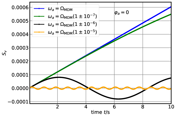
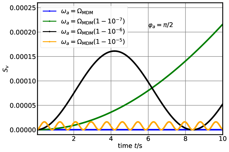
Figure 2: Vertical spin component $S_{v}$ as a function of time $t$ for $\varphi_{a}=0$ (upper plot) and $\varphi_{a}=\pi/2$ (lower plot) and for different axion frequencies $\omega_{a}$ and $\Omega_{\mathrm{MDM}}=750000.0\,$\mathrm{s}^{-1}$$, $\Omega_{\mathrm{EDM}}\approx 1200000\,$\mathrm{s}^{-1}$$, $\eta_{0}=0$, $\eta_{1}=10^{-10}$.

3 Statistical Error Estimates

Equations 11 and 12 can now be used to calculate statistical sensitivities under various experimental conditions. We are interested in the error on $\eta_{1}$.

3.1 Resonance case

The best sensitivity is of course given on resonance, i.e. $\Omega_{\mathrm{MDM}}=\omega_{a}$. In this case the spin build-up follows equation 12:

$$S_{v}(t)=\eta_{1}\frac{\Omega_{\mathrm{EDM}}}{2}\cos(\varphi_{a})t\,.$$ (14)

Assuming that one extracts a beam of $N$ particles continuously on a target with the same rate over a time period $T$ during which the beam polarisation $P$ is assumed to be constant and using a polarimeter with an average analyzing power $A$ of the scattering process and a fraction $f$ of the beam particles detected, the observed vertical polarization (assuming $P_{v}\ll P$) will be:

$$P_{v}(t)=PAS_{v}(t)=PA\eta_{1}\frac{\Omega_{\mathrm{EDM}}}{2}\cos(\varphi_{a})t\,.$$ (15)

From this polarization measurement $\eta_{1}$ can be determined with variance

$$V(\eta_{1})=\left(\frac{1}{\Omega_{\mathrm{EDM}}}\right)^{2}\,\frac{96}{fN(ATP\cos(\varphi_{a}))^{2}}\,.$$ (16)

Details are given in Appendix B.1.

Adding the information from the two bunches with $\Delta\varphi_{a}=\pi/2$ one arrives at

$$V(\eta_{1})=\left(\frac{1}{\Omega_{\mathrm{EDM}}}\right)^{2}\,\frac{96}{fN(ATP)^{2}}\,.$$ (17)

3.2 Off-resonance case

For the off-resonance case the vertical polarisation is obtained by multiplying equation 11 with $PA$:

$$~{}P_{v}(t)=\eta_{1}PA\frac{\Omega_{\mathrm{EDM}}}{2\Delta\omega}\left(-\sin(\varphi_{a})+\sin(\Delta\omega t+\varphi_{a})\right)\,.$$ (18)

In order to determine $\eta_{1}$, the data have to be fitted to the functional form of equation 18. The three fit parameter are $\eta_{1}$, $\Delta\omega$ and $\varphi_{a}$.

The central red curve in Figure 3 shows the figure of merit (FOM) defined as the inverse of the variance of $\eta_{1}$ as a function of $\Delta\omega T/(2\pi)$ normalized to the FOM at resonance $\Delta\omega=\omega_{a}-\Omega_{\mathrm{MDM}}=0$ given by the inverse of equation 17. If the frequency is off be $1/T$, with $T$ being the measurement duration, the FOM drops to roughly 20%. Details are given in appendix B.2. This suggests to take measurements separated by $1/T$ in frequency, as indicated by the additional blue and green FOM curves in Figure 3. The upper dashed black curve which is roughly constant shows the sum of the FOMs from the measurements at the different frequencies. Experimentally one would not run at frequencies $\Delta\omega T/(2\pi)=\dots,-2,-1,0,1,2,\dots$ as indicated in Figure 3 but rather sweep the frequency with the speed (=frequency per time) $v=1/T^{2}$.

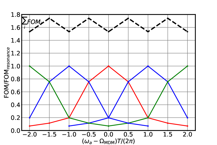
Figure 3: Figure of merit (FOM) as a function of $(\omega_{a}-\Omega_{\mathrm{MDM}})T/(2\pi)$ normalized to the FOM at resonance $\Delta\omega=(\omega_{a}-\Omega_{\mathrm{MDM}})=0$. Solid lines: FOM for measurements at $\Delta\omega T/(2\pi)=-2,-1,0,1,2$ respectively. Dashed line: sum of FOMs.

To scan a region of $\Delta f=1\,$\mathrm{k}\mathrm{H}\mathrm{z}$$ with a measurement duration of $T=10\,$\mathrm{s}$$ for a single frequency, one would thus need a total measurement time

$$\Delta fT^{2}=10^{5}\,$\mathrm{s}$\,.$$

In this frequency range $\eta_{1}$ would be determined with the same accuracy over the whole frequency range.

3.3 Estimates for the error on the axion-gluon coupling $\frac{C_{G}}{f_{a}}$

According to reference Dragos:2019oxn the relation between the EDM $d$ and $\theta_{QCD}$ is given by $d\approx 10^{-16}\theta_{QCD}e\,$\mathrm{c}\mathrm{m}$$. To simplify the discussion we make no distinction between proton and deuteron. $\theta_{QCD}$ is connected to the axion field amplitude $a_{0}$ and the axion-gluon coupling strength $C_{g}/f_{a}$ via $\theta_{QCD}=a_{0}\,C_{g}/f_{a}$. Using the relation between the axion density $\rho_{a}$ to the amplitude $a_{0}=\sqrt{2\rho_{a}}/m_{a}$ and finally equating $\rho_{a}$ with the local dark matter density $\rho_{LDM}\approx 0.4$\mathrm{G}\mathrm{e}\mathrm{V}\mathrm{/}\mathrm{c}\mathrm{m}^{3}$\approx 3\cdot 10^{-42}$\mathrm{G}\mathrm{e}\mathrm{V}^{4}$$ (see reference Tanabashi:2018oca ), assuming that axions saturate the local DM energy, accuracy estimates for $C_{g}/f_{a}$ can be obtained as a function of the axion mass $m_{a}$:

$$d^{osc.} = 10^{-16}\,\theta_{QCD}\,e\,$\mathrm{c}\mathrm{m}$$$ (19)

$$= 10^{-16}\,a_{0}\,\frac{C_{G}}{f_{a}}$$ (20)

$$= 10^{-16}\,\frac{\sqrt{2\rho_{LDM}}}{m_{a}}\,\frac{C_{G}}{f_{a}}$$ (21)

$$= 2.5\cdot 10^{-18}\,\frac{C_{G}}{f_{a}}\frac{1}{m_{a}}\,e$\mathrm{V}$\,$\mathrm{G}\mathrm{e}\mathrm{V}$\,e$\mathrm{c}\mathrm{m}$=\eta_{1}\frac{q\hbar}{2mc}\,S\,.$$ (22)

Table 1 gives an overview over frequency ranges accessible at the existing Cooler Synchrotron COSY at Forschungszentrum Jülich in Germany using polarized protons and deuterons and for a planned prototype storage ring with combined electric and magnetic bending fields for an EDM measurement Abusaif:2018oly . Other parameters, like number of stored particles $N$, efficiency $f$, analyzing power $A$, polarization $P$ and spin coherence time $\tau$ are given as well.

		COSY				prototype ring
		proton		deuteron		proton
momentum	$p/$\mathrm{G}\mathrm{e}\mathrm{V}$/c$	0.3	3.7	0.3	3.7	0.25	0.30
spin revolution frequency	$\Omega_{\mathrm{MDM}}$/ $\mathrm{1}\mathrm{0}^{6}\,\mathrm{s}^{-1}$	5.86	72.3	0.233	2.88	7.35	0.0
axion mass	$m_{a}$/$\mathrm{e}\mathrm{V}$	$4\cdot 10^{-9}$	$5\cdot 10^{-8}$	$1.5\cdot 10^{-10}$	$2\cdot 10^{-9}$	$5\cdot 10^{-9}$	0
magnetic field	$B/$\mathrm{T}$$	0.07	0.8	0.07	0.8	0.0	0.033
electric field	$E/$\mathrm{M}\mathrm{V}\mathrm{/}\mathrm{m}$$	$-$	$-$	$-$	$-$	7.4	7.4
stored particles per bunch	$N$	$10^{9}$				$10^{10}$
fraction detected events	$f$	0.005				0.005
average analyzing power	$A$	0.6				0.5
beam polarization	$P$	0.8				0.8
spin coherence time	$\tau\,/$\mathrm{s}$$	1000				1000

Table 1: Parameters used for the estimates. The ring radius of the prototype ring is $R=8.9\,$\mathrm{m}$$.

The accuracy estimates are given for two scenarios

1. One year of beam time ($10^{7}$\mathrm{s}$$) is spent at a single frequency.

2. In one year of beam time a certain range in frequency is covered.

For the duration of a single measurement, we assure that it does not exceed the axion coherence time, $\tau_{ax}$, given by

$$\tau_{ax}=\frac{\pi\hbar}{m_{a}}Q$$

with a quality factor $Q=3\cdot 10^{6}$ as in reference Chang:2019poy .

The dots in Fig. 4 indicate one-$\sigma$ limits one could reach at COSY running with protons or deuterons and for the prototype ring running at one fixed frequency for one year for each point.

In the second scenario we start with the total running time available in one year, $T_{y}=10^{7}\,$\mathrm{s}$$. For the prototype ring, if one wants to span a region of $\Delta f=1\,$\mathrm{M}\mathrm{H}\mathrm{z}$$ in one year, the duration $T$ is given by

$$T=\sqrt{\frac{T_{y}}{\Delta f}}=3.2\,$\mathrm{s}$\,.$$

for each frequency interval $\Delta f_{i}={1}/{T}$. For a $1\,$\mathrm{k}\mathrm{H}\mathrm{z}$$ region, one finds $T=100\,$\mathrm{s}$$.

The corresponding limits are shown in Fig. 4 as colored areas. The green line shows estimates from reference Chang:2019poy scaled to match them with the assumptions made in this document about the parameters $N,f,P,A$.

The same is shown for running at COSY. The fact that the limits using a pure magnetic ring are getting worse at smaller frequency is due to the fact that for lower frequencies, the magnetic field is lower, which in turns makes $\Omega_{\mathrm{EDM}}$ smaller and one looses sensitivity. For the combined ring the electric field is constant, a small magnetic field is added to slow down the spin precession. $\Omega_{\mathrm{EDM}}$ varies only very little.

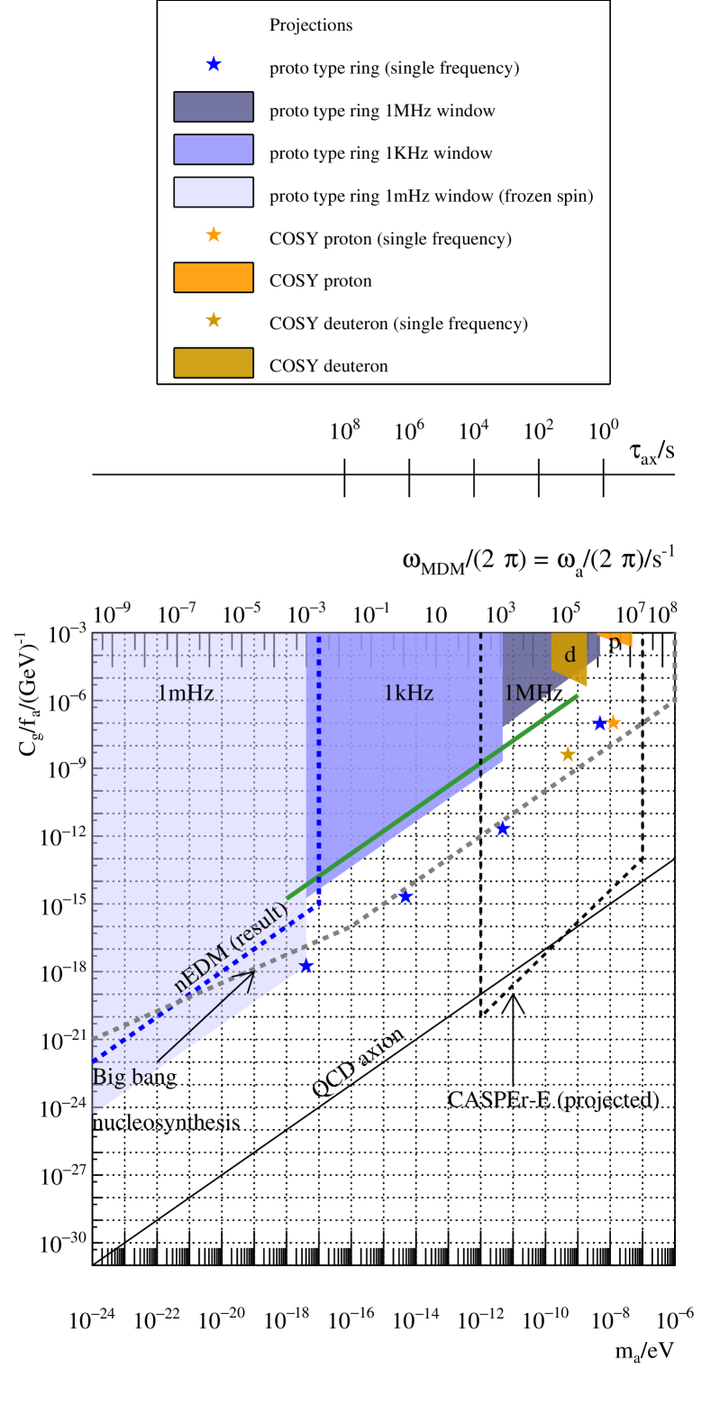
Figure 4: One $\sigma$ limits for the axion-gluon coupling $C_{g}/f_{a}$ reachable within one year running at a fixed frequency (stars) or over a given frequency range (areas) for COSY (orange) or the prototype ring (blue). In addition limits reached by the nEDM experiments Abel:2017rtm , nucleosynthesis Blum:2014vsa and prospects for NMR experiments Budker:2013hfa are shown schematically. The green line shows the estimates obtained in Chang:2019poy with simulations.

4 Summary and conclusion

Analytic expressions for the spin motion in presence of an oscillating EDM in storage rings were derived from the Thomas-BMT equation. These were used to give sensitivity estimates for the axion-gluon coupling at COSY and at a prototype EDM ring. This was done for two scenarios: 1.) Running at one fixed frequency, 2.) covering a wide range in frequency.

The results are in good agreement compared to reference Chang:2019poy where a numerical approach was used to find sensitivities.

Appendix A Solution of equation 7

Equation 7 can be written as

$$\dot{\vec{S}}=(A_{\mathrm{MDM}}+\eta\tilde{A}_{\mathrm{EDM}}(t))\vec{S}\,.$$ (23)

To solve equation 23 we expand the solution in orders of $\eta$

$$\vec{S}(t)=\vec{S}_{0}(t)+\eta\vec{S}_{1}(t)$$ (24)

Entering equation 24 in equation 23 and keeping only terms up to order one in $\eta$ yields

$$\dot{\vec{S}}_{0}+\eta\dot{\vec{S}}_{1}=A_{\mathrm{MDM}}\vec{S}_{0}+\eta(A_{\mathrm{MDM}}\vec{S}_{1}+\tilde{A}_{\mathrm{EDM}}\vec{S}_{0})\,.$$ (25)

Thus

$$\dot{\vec{S}}_{0} = A_{\mathrm{MDM}}\vec{S}_{0}\,,$$ (26)

$$\dot{\vec{S}}_{1} = (A_{\mathrm{MDM}}\vec{S}_{1}+\tilde{A}_{\mathrm{EDM}}\vec{S}_{0})\,.$$ (27)

Since $A_{\mathrm{MDM}}$ does not depend on $t$, equation 26 has the solution

$$\vec{S}_{0}(t)=\mathrm{exp}(A_{\mathrm{MDM}}t)\vec{S}(0)$$ (28)

with arbitrary initial condition $\vec{S}(0)$.

The solution for the equation 27 can be found using the variation of constant method:

$$S_{1}=\mathrm{exp}(A_{\mathrm{MDM}}t)S(0)+\int_{0}^{t}\mathrm{exp}(A_{\mathrm{MDM}}(t-s))\tilde{A}_{\mathrm{EDM}}S_{0}(t)\mathrm{d}s\,.$$ (29)

Up to first order in $\eta$ the solution is

$$\vec{S}(t) = \vec{S}_{0}(t)+\eta\vec{S}_{1}(t)$$ (30)

$$= (1+\eta)\,\mathrm{exp}(A_{\mathrm{MDM}}t)\,\vec{S}(0)+\eta\,\int_{0}^{t}\mathrm{exp}(t-s)\tilde{A}_{\mathrm{EDM}}\mathrm{exp}(A_{\mathrm{MDM}}t)\,\vec{S}(0)\mathrm{d}s$$ (31)

Using Mathematica Mathematica one finds $\vec{S}(t)=A(t)\vec{S}(0)$ with

$$A_{11} = (1+\eta_{0})\cos(\Omega_{\mathrm{MDM}}t)\hskip 227.62204pt$$ (32)

$$A_{12} = \frac{\eta_{0}\Omega_{\mathrm{EDM}}(\cos(\Omega_{\mathrm{MDM}}t)-1)}{\Omega_{\mathrm{MDM}}}$$ (33)

$$+ \,\eta_{1}\Omega_{\mathrm{EDM}}\,\Big{(}\frac{(\sin(\varphi_{a})(\omega_{a}\sin(\Omega_{\mathrm{MDM}}t)-\Omega_{\mathrm{MDM}}\sin(\omega_{a}t))}{\omega_{a}^{2}-\Omega_{\mathrm{MDM}}^{2}}$$

$$\hskip 42.67912pt+\frac{\Omega_{\mathrm{MDM}}\cos(\varphi_{a})(\cos(\omega_{a}t)-\cos(\Omega_{\mathrm{MDM}}t))}{\omega_{a}^{2}-\Omega_{\mathrm{MDM}}^{2}}\Big{)}$$

$$A_{13} = (1+\eta_{0})\sin(\Omega_{\mathrm{MDM}}t)$$ (34)

$$A_{21} = \frac{\eta_{0}\Omega_{\mathrm{EDM}}(\cos(\Omega_{\mathrm{MDM}}t)-1)}{\Omega_{\mathrm{MDM}}}$$ (35)

$$- \eta_{1}\Omega_{\mathrm{EDM}}\Big{(}\frac{(\cos((\omega_{a}-\Omega_{\mathrm{MDM}})t+\varphi_{a})}{2(\omega_{a}-\Omega_{\mathrm{MDM}})}$$

$$\hskip 42.67912pt+\frac{(\Omega_{\mathrm{MDM}}-\omega_{a})\cos((\omega_{a}+\Omega_{\mathrm{MDM}})t+\varphi_{a})-2\Omega_{\mathrm{MDM}}\cos(\varphi_{a}))}{2(\omega_{a}-\Omega_{\mathrm{MDM}})(\omega_{a}+\Omega_{\mathrm{MDM}})}\Big{)}$$

$$A_{22} = 1+\eta_{0}$$ (36)

$$A_{23} = \frac{\eta_{0}\Omega_{\mathrm{EDM}}\sin(\Omega_{\mathrm{MDM}}t)}{\Omega_{\mathrm{MDM}}}$$ (37)

$$+ \eta_{1}\Omega_{\mathrm{EDM}}\Big{(}\frac{(\sin((\omega_{a}-\Omega_{\mathrm{MDM}})t+\varphi_{a})}{2(\omega_{a}-\Omega_{\mathrm{MDM}})}$$

$$\hskip 42.67912pt+\frac{(\omega_{a}-\Omega_{\mathrm{MDM}})\sin((\omega_{a}+\Omega_{\mathrm{MDM}})t+\varphi_{a})-2\omega_{a}\sin(\varphi_{a}))}{2(\omega_{a}-\Omega_{\mathrm{MDM}})(\omega_{a}+\Omega_{\mathrm{MDM}})}\Big{)}$$

$$A_{31} = -(1+\eta_{0})\sin(\Omega_{\mathrm{MDM}}t)$$ (38)

$$A_{32} = -\frac{\eta_{0}\Omega_{\mathrm{EDM}}\sin(\Omega_{\mathrm{MDM}}t)}{\Omega_{\mathrm{MDM}}}$$ (39)

$$+ \eta_{1}\Omega_{\mathrm{EDM}}\,\Big{(}\frac{(\omega_{a}\sin(\varphi_{a})\cos(\Omega_{\mathrm{MDM}}t)-\omega_{a}\sin(\omega_{a}t+\varphi_{a})}{(\omega_{a}-\Omega_{\mathrm{MDM}})(\omega_{a}+\Omega_{\mathrm{MDM}})}$$

$$\hskip 42.67912pt+\frac{\Omega_{\mathrm{MDM}}\cos(\varphi_{a})\sin(\Omega_{\mathrm{MDM}}t))}{(\omega_{a}-\Omega_{\mathrm{MDM}})(\omega_{a}+\Omega_{\mathrm{MDM}})}\Big{)}$$

$$A_{33} = (1+\eta_{0})\cos(\Omega_{\mathrm{MDM}}t)$$ (40)

Note that $\eta=\eta_{0}+\eta_{1}\cos(\omega_{a}t+\varphi_{a})$. We are mainly interested in the entries $A_{23}$ and $A_{21}$ which gives the vertical polarisation in case of an initial in plane polarisation.

Appendix B Variance on $\eta_{1}$

B.1 Resonance case: variance of a slope

Starting point is equation 15

$$P_{v}(t)=PAS_{v}(t)=PA\eta_{1}\frac{\Omega_{\mathrm{EDM}}}{2}\cos(\varphi_{a})\,t.$$ (41)

The variance on the slope parameter $s=PA\eta_{1}\frac{\Omega_{\mathrm{EDM}}}{2}\cos(\varphi_{a})$ of a straight line is

$$V(s)=\frac{\sigma^{2}}{N_{\mathrm{points}}V(t)}\,,$$

where $\sigma$ is the error on each individual point where the curve is measured. $N_{points}$ is the number of points entering the fit and $V(t)$ is the variance of the points along the time axis. For evenly distributed values in a time interval $T$, one has $V(t)=T^{2}/12$. If the polarization is determined from an azimuthal asymmetry one has Pretz:2018bze :

$$\sigma^{2}=\frac{2}{n}\,,$$

where $n$ is the number of events entering the analysis for a single point. Evidently for the total number of events one has $Nf=nN_{points}$.

Putting everything together one finds

$$V(s)=\frac{24}{fNT^{2}}\,.$$ (42)

Translated to the variance on $\eta_{1}$ one finds the expression given in equation 17

$$V(\eta_{1})=\frac{24}{fN(PAT\cos(\varphi_{a}))^{2}}\left(\frac{2}{\Omega_{\mathrm{EDM}}}\right)^{2}\,.$$ (43)

B.2 Off-resonance case: variance of an amplitude

A polarization given by equation 18 leads to the following count rate in the detector:

$$N(t)\propto 1+\eta_{1}\frac{PA\Omega_{\mathrm{EDM}}}{2\Delta\omega}\,\left(-\sin(\varphi_{a})+\sin(\Delta\omega t+\varphi_{a})\right)\cos(\Phi)$$ (44)

where $\Phi$ is the azimuthal angle of the scattered particle. There are three unknowns $\eta_{1}$, $\Delta\omega$ and $\varphi_{a}$. To estimate the uncertainty on $\eta_{1}$ we consider the extended maximum likelihood method applied to the counting rate in equation 44. The log-likelihood function $\ell$ has the form

$$\ell=\sum_{i=1}^{N_{\mathrm{events}}}\log\left(1+\eta_{1}\frac{PA\Omega_{\mathrm{EDM}}}{2\Delta\omega}\left(-\sin(\varphi_{a})+\sin(\Delta\omega t+\varphi_{A})\right)\cos(\Phi_{i})\right)-\log(N_{tot})\,,$$ (45)

where $N_{tot}$ is the total number of events detected.

To get the covariance matrix for the three unknowns $\eta_{1},\Delta\omega$ and $\varphi_{a}$ one has to consider the expectation values of the second derivatives of the likelihood function.

The the second derivative with respect to $\eta_{1}$ it is for example given by

$$\left<\frac{\partial^{2}\ell}{\partial\eta_{1}^{2}}\right>=\int_{0}^{T}\frac{\partial^{2}\ell}{\partial\eta_{1}^{2}}N(t)\mathrm{d}t\,.$$ (46)

For $\eta_{1}/\Delta\omega\ll 1$ and a measurement time $T=2\pi/\Delta\omega$ (corresponding roughly to the black curves in Figure 2), one finds for example for the error on $\eta_{1}$:

$$\sigma_{\varphi_{a}=0}^{2} = \frac{1}{(\Omega_{\mathrm{EDM}}ATP)^{2}fN}\,\frac{128\pi^{2}(15+2\pi^{2})}{(3+4\pi^{2})}\approx\frac{1033}{(\Omega_{\mathrm{EDM}}ATP)^{2}fN}$$

$$\quad\mbox{for}\,\,\varphi_{a}=0\,,$$

$$\sigma_{\varphi_{a}=\pi/2}^{2} = \frac{1}{(\Omega_{\mathrm{EDM}}ATP)^{2}fN}\,\frac{128\pi^{2}(15-2\pi^{2})}{33-4\pi^{2}}\approx\frac{924}{(\Omega_{\mathrm{EDM}}ATP)^{2}fN}\,$$

$$\quad\mbox{for}\,\,\varphi_{a}=\frac{\pi}{2}\,.$$

Combining these two measurements leads to a

$$V(\eta_{1})=\frac{488}{(\Omega_{\mathrm{EDM}}ATP)^{2}fN}\$$ (49)

which is approximately a factor 5 larger compared to the resonance case in equation 43.

References

- (1) S. P. Chang, S. Haciomeroglu, O. Kim, S. Lee, S. Park, and Y. K. Semertzidis, “Axionlike dark matter search using the storage ring EDM method,” Phys. Rev., vol. D99, no. 8, p. 083002, 2019.
- (2) P. W. Graham, I. G. Irastorza, S. K. Lamoreaux, A. Lindner, and K. A. van Bibber, “Experimental Searches for the Axion and Axion-Like Particles,” Ann. Rev. Nucl. Part. Sci., vol. 65, pp. 485–514, 2015.
- (3) I. G. Irastorza and J. Redondo, “New experimental approaches in the search for axion-like particles,” Prog. Part. Nucl. Phys., vol. 102, pp. 89–159, 2018.
- (4) P. W. Graham and S. Rajendran, “New Observables for Direct Detection of Axion Dark Matter,” Phys. Rev., vol. D88, p. 035023, 2013.
- (5) D. Budker, P. W. Graham, M. Ledbetter, S. Rajendran, and A. Sushkov, “Proposal for a Cosmic Axion Spin Precession Experiment (CASPEr),” Phys. Rev., vol. X4, no. 2, p. 021030, 2014.
- (6) V. Anastassopoulos et al., “A Storage Ring Experiment to Detect a Proton Electric Dipole Moment,” Rev. Sci. Instrum., vol. 87, no. 11, p. 115116, 2016.
- (7) F. Abusaif et al., “Storage Ring to Search for Electric Dipole Moments of Charged Particles - Feasibility Study,” 2019.
- (8) V. Bargmann, L. Michel, and V. L. Telegdi, “Precession of the polarization of particles moving in a homogeneous electromagnetic field,” Phys. Rev. Lett., vol. 2, pp. 435–436, 1959.
- (9) D. F. Nelson, A. A. Schupp, R. W. Pidd, and H. R. Crane, “Search for an Electric Dipole Moment of the Electron,” Phys. Rev. Lett., vol. 2, pp. 492–495, 1959.
- (10) T. Fukuyama and A. J. Silenko, “Derivation of Generalized Thomas-Bargmann-Michel-Telegdi Equation for a Particle with Electric Dipole Moment,” Int. J. Mod. Phys., vol. A28, p. 1350147, 2013.
- (11) P. W. Graham and S. Rajendran, “Axion Dark Matter Detection with Cold Molecules,” Phys. Rev., vol. D84, p. 055013, 2011.
- (12) J. Dragos, T. Luu, A. Shindler, J. de Vries, and A. Yousif, “Confirming the Existence of the strong CP Problem in Lattice QCD with the Gradient Flow,” 2019.
- (13) M. Tanabashi et al., “Review of Particle Physics,” Phys. Rev., vol. D98, no. 3, p. 030001, 2018.
- (14) F. Abusaif et al., “Feasibility Study for an EDM Storage Ring,” 2018.
- (15) C. Abel et al., “Search for Axionlike Dark Matter through Nuclear Spin Precession in Electric and Magnetic Fields,” Phys. Rev., vol. X7, no. 4, p. 041034, 2017.
- (16) K. Blum, R. T. D’Agnolo, M. Lisanti, and B. R. Safdi, “Constraining Axion Dark Matter with Big Bang Nucleosynthesis,” Phys. Lett., vol. B737, pp. 30–33, 2014.
- (17) W. R. Inc., “Mathematica, Version 12.0.” Champaign, IL, 2019.
- (18) Pretz, J. and Müller, F., “Extraction of Azimuthal Asymmetries using Optimal Observables,” Eur. Phys. J., vol. C79, no. 1, p. 47, 2019.