Polynomials of genus one prime knots
of complexity at most five
Abstract.
Prime knots of genus one admitting diagram with at most five classical crossings were classified by Akimova and Matveev in 2014. In 2018 Kaur, Prabhakar and Vesnin introduced families of -polynomials and -polynomials for virtual knots which are generalizations of affine index polynomial. Here we introduce a notion of totally flat-trivial knots and demonstrate that for such knots -polynomials and -polynomials coincide with affine index polynomial. We prove that all Akimova – Matveev knots are totally flat-trivial and calculate their affine index polynomials.
Key words and phrases:
Virtual knot, knot in a thickened torus, affine index polynomial2010 Mathematics Subject Classification:
57M27Introduction
Tabulating of virtual knots and constructing their invariants is one of the key problems in mordern low-dimensional topology. Table of virtual knots with diagrams, having at most four classical crossings may be found in monography [3] and online [4]. Due to equivalence of virtual knots and knots in thickened surfaces, it’s interesting to consider tabulation of knots in 3-manifolds, which are thickenings of surfaces of certain genus. Up to now, there are just few results in this direction. Here we consider prime knots of genus one, admitting diagrams with small number of classical crossings, tabulated by Akimova and Matveev in [1].
We are intrested in behaviour of several polynomial invariants on Akimova – Matveev knots. Recall that Kaufman in [7] defined an afiine index polynomial which is an invariant of a virtual knot and possess some important proprties [8]. In [9] a generalization of affine index polynomials was introduced, namely a family of -polynomials and family of -polynomials . In [5] authors, using their software, calculated -polynomials of knots tabulated in [3] and [4]. Here we consider polynomial invariants for knots in a thickened torus.
The paper has the following structure: in Section 1 we recall some basic definitions and facts to use further, in Section 2 we introduce totally flat-trivial knots and show that for these knots -polynomials and -polynomials coincide with affine index polynomial, in Section 3 we calculate these invariants for Akimova – Matveev knots. In Theorem 3.1 we show that Akimova – Matveev knots are totally flat-trivial. In Corollary 3.2 and Table 2 their affine index polynomials are given. The investigation of properties of Akimova – Matveev knots leads to the following Question 3.3: Is it true, that every virtual knot of genus one is totally flat-trivial?
1. Basic definitions
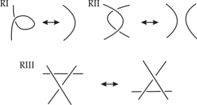
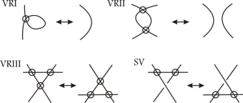
Virtual knots and links were introduced by Louis Kaufman in [6] as an essential generalization of classical knots. Diagrams of virtual knots may have classical and virtual crossings both. Two virtual knots are equivalent if and only if their diagrams could be transformed in each other by finite sequences of classical (RI, RII, RIII in Fig. 1) and virtual (VRI, VRII, VRIII and SV in Fig. 2) Reidemeister moves.
Diagram, obtained by forgetting over/under crossing information is said to be flat knot diagram. Equivalence of flat knots is defined by flat Reidemeister moves, which are different from virtual Reidemeister moves in having flat crossings instead of classical ones.
Let be a diagram of an oriented virtual knot. We denote the set of all classical crossings of diagram as . Sign of a classical crossing, denoted by is defined as shown in the Fig. 3.
For every arc in a diagram of virtual knot we assign an integer value in such way that relations presented in a picture4 hold. In [7] Kaufman proved, that such coloring of an oriented virtual knot diagram, called Cheng coloring, always exists. Indeed, for every arc of a diagram one can assign value , where is the set of classical crossings, which are fist met as overcrossings, when moving around the knot from with respect to the orientation.
In [2] Cheng and Gao put every classical crossing in correspondence with an integer value , defined as
| (1) |
where and given by Cheng coloring. One can notice, that Cheng coloring does not depend on types of classical crossings and hence it is defined for an oriented flat knot diagram. Let us remember that affine index polynomial from [7] can be written in the following form:
| (2) |
where is a set of all classical crossings of .
In [11] Satoh and Taniguchi introduced a notion of -writhe . For every define -writhe of oriented virtual knot diagram as a difference between number of positive crossings and negative crossings of index . Notice that is a coefficient of in affine index polynomial and it is an invariant of oriented virtual knot. For more information about -writhe see [11]. Using -writhe in [9] was defined another invariant – -dwrithe :
Remark 1.1.
is an invariant of oriented virtual knot, since is an invariant of oriented virtual knot. Moreover, for every classical knot.
As it shown in [9], represents a flat knot structure. Namely, the following lemma holds
Lemma 1.2.
[9, Lemma 2.4] For every , -dwrithe is an oriented flat knot invariant.
Let be a diagram, obtained from by reversing an orientation and is obtained by switching all classical crossings.
Lemma 1.3.
[9, Lemma 2.5] Let be a diagram of oriented virtual knot, then and .
Consider a smoothing according to the rule, shown in picture 5. We will call this kind of smoothing by smoothing against orientation. Orientation of is induced by smoothing. Since is a diagram of virtual knot, so is a diagram of virtual knot too.
Definition 1.4.
[9] For a diagram of a virtual oriented knot and an integer , a polynomial is defined as:
| (3) |
Note that -polynomials generalize affine index polynomial, since for every and every .
Definition 1.5.
[9] For a diagram of a virtual oriented knot and an integer , a polynomial is defined as:
| (4) |
where .
Theorem 1.6.
[9] For every integer polynomials and are oriented virtual knot invariants.
2. Totally flat-trivial knots
Let be a diagram of oriented virtual knot and a set of all classical crossings in .
Definition 2.1.
We will call totally flat-trivial if diagrams obtained from and for all by forgetting over/under crossing information are flat equivalent to unknot. Virtual knot is said to be totally flat-trivial, if it admits a totally flat-trivial diagram.
Lemma 2.2.
If virtual knot is totally flat-trivial, then
-
(1)
For all we have and .
-
(2)
is palindromic.
Proof.
(1) Let be a totally flat-trivial diagram of a knot , a set of all its classical crossings, and a diagram, obtained by smoothing against orientation in crossing . By the definition, all these diagrams are flat-equivalent to a trivial knot. By Lemma 1.2 we have and for all . From these equalities and formulas (2), (3), and (4) we obtain that
(2) It was mentioned above that is a coefficient of in affine index polynomial. By the equality , coefficients of and coincide and is palindromic. ∎
Recall the following properties of affine index polynomial. Let be a diagram, obtained from by reversing orientation and is obtained by switching all classical crossings.
Lemma 2.3.
[7] The following equalities hold
3. Polynomial invariants of Akimova-Matveev knots
Prime knots in thickened torus , that is a product of 2-dimensional torus and the unit interval , admitting diagrams with at most five classical crossings were tabulated by Akimova and Matveev in [1]. The total number of these diagrams is equal to . Due to Kuperberg’s result [10], it is equivalent to tabulating prime virtual knots of genus one. To distinguish the knots, Akimova and Matveev introduced for diagrams on a torus an analogue of bracket polynomial. These diagrams, pictured on a plane using virtual crossing are given in [1, Fig. 17]. For reader’s convenience we present them in Tables 3 and 4.
Theorem 3.1.
Every Akimova –Matveev knot is totally flat-trivial.
Proof.
It’s easy to see, that forgetting the information of over/under crossings in diagrams from Tables 3 and 4 leads us to 40 different diagrams of flat knots as in Table 1.
| knot | knot | knot | knot | knot | |||||
| 1 | 2.1 | 9 | 4.10, 4.11 | 17 | 5.10 | 25 | 5.23, 5.24 | 33 | 5.40-5.42 |
| 2 | 3.1 | 10 | 4.12-4.14 | 18 | 5.11 | 26 | 5.25, 5.26 | 34 | 5.43-5.46 |
| 3 | 3.2, 3.3 | 11 | 4.15-4.17 | 19 | 5.12 | 27 | 5.27-5.29 | 35 | 5.47-5.50 |
| 4 | 4.1 | 12 | 5.1, 5.2 | 20 | 5.13 | 28 | 5.30 | 36 | 5.51-5.53 |
| 5 | 4.2 | 13 | 5.3, 5.4 | 21 | 5.14 | 29 | 5.31 | 37 | 5.54-5.59 |
| 6 | 4.3 | 14 | 5.5 | 22 | 5.15, 5.16 | 30 | 5.32, 5.33 | 38 | 5.60-5.65 |
| 7 | 4.4, 4.5 | 15 | 5.6, 5.7 | 23 | 5.17, 5.18 | 31 | 5.34-5.37 | 39 | 5.66-5.68 |
| 8 | 4.6-4.9 | 16 | 5.8, 5.9 | 24 | 5.19-5.22 | 32 | 5.38, 5.39 | 40 | 5.69 |
Further we consider each of these classes separately and prove them to be totally flat-trivial. Changing type of a crossing leads to changing in orientation of a knot, obtained by smoothing at the crossing. Thereby it is sufficient to consider just one member from each of 40 classes to prove the theorem for the all 90 knots.
As an example we consider a virtual knot pictured in Fig. 6.

It’s easy to see, that it is flat-trivial. Then we consider all the diagrams obtained by smoothings in classical crossings. There are five classical crossings denoted as , , , , . Diagrams, obtained by smoothings at , and are shown in the picture 7.


As one can see, all diagrams in Fig. 7 are also flat-trivial. Similarly, diagrams obtained by smoothing at and are also flat-trivial. Hence, virtual knot is totally flat-trivial. Analogous considerations for knots from other classes show that they are all totally flat-trivial, and thus all Akimova-Matveev knots are totally flat-trivial. ∎
Theorem 3.1 and Lemma 2.2 allow us o obtain the following properties of -polynomials, -polynomials and affine index polynomial of Akimova – Matveev knots.
Corollary 3.2.
Let be a genus one knot admitting a diagram with at most five crossings. Then for every its polynomials and -polynomials coincide with affine index polynomial, presented in Table 2, where knots are splitted in groups with respect to the value of polynomials for the knot or its mirror image .
| knot | polynomial |
|---|---|
| 4.4, 4.5, 5.15, 5.16, 5.27, 5.28, 5.29, 5.30, | |
| 5.31, 5.45, 5.47, 5.48, 5.67, 5.69 | |
| 2.1, 3.1, 4.2, 5.6, 5.7*, 5.10*, 5.13*, 5.19, | |
| 5.20, 5.21*, 5.22, 5.23, 5.24*, 5.43, 5.46 | |
| 4.1*, 4.3, 5.5, 5.12, 5.44 | |
| 3.2, 3.3, 4.6, 4.9, 4.10, 4.11, 5.3, 5.4*, 5.8, 5.9*, | |
| 5.14, 5.17, 5.18*, 5.32, 5.33, 5.34, 5.37, 5.49, 5.66 | |
| 5.1, 5.2, 5.11, 5.25, 5.26, 5.50, 5.68 | |
| 4.8, 5.35*, 5.39* | |
| 4.7, 5.36, 5.38 | |
| 4.13, 4.15, 4.16, 4.17, 5.40, 5.41, 5.42*, 5.52, 5.53* | |
| 4.14 | |
| 4.12, 5.51 | |
| 5.54, 5.57, 5.60, 5.61, 5.62, 5.63, 5.64*, 5.65 | |
| 5.56, 5.68* | |
| 5.55, 5.59 |
Question 3.3.
Is it true, that every virtual knot of genus one is totally flat trivial?
References
- [1] A.A. Akimova, S.V. Matveev, Classification of genus 1 virtual knots having at most five classical crossings, Journal of Knot Theory and Its Ramificatons 23(6) (2014).1450031 (19 pages).
- [2] Z. Cheng, H. Gao, A polynomial invariant of virtual links, Journal of Knot Theory and Its Ramifications 22(12) (2013), 1341002.
- [3] H. Dye, An invitation to knot theory: virtual and classical. 2016.
- [4] J. Green, A table of virtual knots, available at https://www.math.toronto.edu /drorbn/Students/GreenJ/ last updated August 10, 2004.
- [5] M. Ivanov, A. Vesnin, -polynomials of tabulated virtual knots, preprint available at arXiv:1906.01976.
- [6] L. Kauffman, Virtual knot theory, European Journal of Combinatorics 20(7) (1999), 663–691.
- [7] L. Kauffman, An affine index polynomial invariant of virtual knots, Journal of Knot Theory and Its Ramifications 22(04) (2013), 1340007.
- [8] L. Kauffman, Virtual knot cobordism and the affine index polynomial, Journal of Knot Theory and Its Ramifications, 27(11) (2018), 1843017.
- [9] K. Kaur, M. Prabhakar, A. Vesnin, Two-variable polynomial invariants of virtual knots arising from flat virtual knot invariants, Journal of Knot Theory and Its Ramifications, 27(13) (2018), 1842015.
- [10] G. Kuperberg, What is a virtual knot? Algebr. Geom. Topol., 3 (2003), 587–591.
- [11] S. Satoh, K. Taniguchi, The writhes of a virtual knot, Fundamenta Mathematicae 225 (2014), 327–341.