Control of discrete-time nonlinear systems via finite-step control Lyapunov functions

Abstract

In this work, we establish different control design approaches for discrete-time systems, which build upon the notion of finite-step control Lyapunov functions (fs-CLFs). The design approaches are formulated as optimization problems and solved in a model predictive control (MPC) fashion. In particular, we establish contractive multi-step MPC with and without reoptimization and compare it to classic MPC. The idea behind these approaches is to use the fs-CLF as running cost. These new design approaches are particularly relevant in situations where information exchange between plant and controller cannot be ensured at all time instants. An example shows the different behavior of the proposed controller design approaches.

1 Introduction

Lyapunov functions are a central tool in the context of nonlinear control theory as they do not only serve as certificates of stability and simplify stability proofs, but also provide means to quantify robustness or redesign the controller to improve robustness of the feedback connection [1]. This has the drawback that systematic methods for obtaining Lyapunov functions for general nonlinear systems still do not exist. In particular, standard Lyapunov function candidates, including quadratic, weighted supremum norm and weighted $1$-norm functions, do not necessarily decay at each time step.

In contrast to classic Lyapunov functions, so-called finite-step Lyapunov functions are energy functions which do not have to decay at each time step, but only after a fixed and finite number of steps. This relaxation leads to significant contributions in the context of stability analysis of (large-scale) nonlinear systems [2, 3, 4, 5, 6]. In particular, it has been shown that any proper scaling of a $p$-norm function is a finite-step Lyapunov function for a large class of asymptotically stable nonlinear systems [2]. Such converse Lyapunov theorems are constructive for control purposes in the sense that they provide an explicit way of construction of a Lyapunov function for control systems. This motivates the use of such results for the controller design in nonlinear control systems. In this paper, we generalize the notion of finite-step Lyapunov functions to control systems by introducing the notion of finite-step control Lyapunov functions (fs-CLF).

Given a fs-CLF, we reformulate a fs-CLF-based control design into an optimization problem. In particular, we link the fs-CLF-based control design to model predictive control (MPC) approaches. By considering three different optimization setups for the fs-CLF-based design, we come up with three fs-CLF-based MPC approaches: a) contractive multi-step MPC; b) contractive updated multi-step MPC; and c) classic (i.e. one-step) MPC. In c), we focus on MPC without terminal constraints and/or costs, see, e.g. [7, Section 7.4] and the references therein for a thorough discussion on MPC with or without additional stabilizing terminal ingredients. In a) and b), the optimization problem includes a contractive condition guaranteeing a decay rate after a finite number of time steps. In all these schemes the running cost in the respective optimization problem is taken as the fs-CLF. The a priori knowledge of such a fs-CLF is guaranteed by the converse Lyapunov theorem stated as Theorem 9 below.

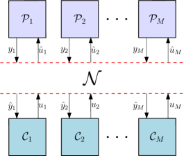
Figure 1: The implementation of $M$ independent control loops over a single communication channel $\mathcal{N}$.

Classic MPC approaches are based on the following philosophy: at each time step we measure the current state value of the system, optimize a cost over the control input using model based predictions of the system response over a fixed optimization horizon, implement the first component of the computed control sequence, and repeat these steps ad infinitum [7]. However, in practice, the controller and the plant may not communicate with each other at each time step. In networked control systems applications, multiple (physically decoupled) plants often need to share a communication channel for exchanging information with their corresponding remotely located controllers; see Figure 1. Therefore only a few plants can exchange information with their controllers at any instant of time and the remaining plants operate in open-loop until they are granted access to the communication channel. The allocation (also known as scheduling) of communication resources is frequently performed in a periodic fashion. In such a situation, we need to develop a control setting in which the controller (if possible) sends not only one component, but a control sequence of the length equal to the periodicity of the allocation process at each transmission instant; see [8, 9] for such networked control systems configurations. Such a scenario motivates our contractive multi-step MPC, where the MPC does not communicate with the plant at each time step, but only after a fixed number of time steps. The whole optimal control sequence is sent to the plant to compensate for the lack of access to the network. To guarantee the stability of the resulting system, we include a contractive constraint, which is obtained from the corresponding fs-CLF, into the optimization problem as an inequality constraint.

Another problem with the classic implementation of MPC is that the execution of the optimization problem at each time step may result in high computational cost (here we assume the controller and the plant can communicate at each time step). To keep the computational cost low, inspired by [10, 11], the second control scheme proposes an updating approach based on re-optimizations on shrinking horizons which are computationally less expensive than re-optimizations on the full horizon in classic MPC schemes. Similar to the first scheme, a contractive constraint is also used in the optimization problem to ensure the stability of the overall system. Finally, the third control scheme proposes a classic MPC approach in which the optimization problem is solved over a fixed optimization horizon at each time step; and hence only the first component of the computed control sequence is applied to the plant. Moreover, the contraction condition is not considered as an additional inequality constraint in the optimization problem. The absence of the contractive constraint reduces the computational complexity, though considering a fixed optimization horizon will increase the computational burden.

The MPC schemes we are proposing have similarities with MPC schemes known from the literature. Particularly, the scheme from Algorithm 11, in which the whole open loop optimal control sequence is used, is an instance of a contractive MPC scheme, as investigated, e.g., in [12, 13, 14, 15]. The contractivity constraint in Problem 10 can be seen as a nonlinear version of the respective condition in [13, 14, 15]. Actually, under suitable conditions the explicit use of a contractive constraint can be replaced by a term in the cost functional with sufficiently high weight, see [16, Theorem 3.18] or [12]. The paper [12] already mentions the possibility to use a fs-CLF in contractive MPC. Contractivity assumptions have also been used in MPC schemes with additional terminal constraints, see [17, 18]. The updating technique with shrinking horizon in Algorithm 15 was inspired by [10, 11], where a theoretical robustness analysis of this method is performed. Finally, the MPC Algorithm 19 without terminal constraints is classical and the particular stability analysis in Theorem 22 uses techniques from [19, 20] (see also [7, Section 6]), which in turn can be seen as a refinement of earlier, similar approaches in [21, 22, 23].

Throughout this paper we consider a stabilization problem with respect to a closed (not necessarily compact) set. This treatment enables us to formulate several stabilization problems in a unified manner.

This paper is organized as follows: First, relevant notation is recalled in Section 2. Then the notion of fs-CLFs together with some other relevant notions are introduced in Section 3. The fs-CLF-based MPC schemes are developed in Section 4. Section 5 concludes the paper.

2 Notation

In this paper, $\mathbb{R}_{\geq 0}(\mathbb{R}_{>0})$ and $\mathbb{N}(\mathbb{N}^{*})$ denote the nonnegative (positive) real numbers and the nonnegative (positive) integers, respectively. For a set $\mathcal{S}\subseteq\mathbb{R}^{n}$, $\operatorname{int}(\mathcal{S})$ and $\operatorname{co}(\mathcal{S})$, respectively, denote the interior and the convex hull of $\mathcal{S}$. Given $\mathcal{S}\subseteq\mathbb{R}^{n}$, $\mathcal{S}^{\ell}:=\underbrace{\mathcal{S}\times\dots\times\mathcal{S}}_{\ell\,\,\mathrm{times}}$ is the $\ell$-fold Cartesian product. The $i$th component of $v\in\mathbb{R}^{n}$ is denoted by $v_{i}$. For any $x\in\mathbb{R}^{n}$, $x^{\top}$ denotes its transpose. We write $(x,y)$ to represent $[x^{\top},y^{\top}]^{\top}$ for $x\in\mathbb{R}^{n},y\in\mathbb{R}^{p}$. For $x\in\mathbb{R}^{n}$, we, respectively, denote the Euclidean norm and the maximum norm by $\left|x\right|$ and by $\left|x\right|_{\infty}$. Given a nonempty set $\mathcal{A}\subset\mathbb{R}^{n}$ and any point $x\in\mathbb{R}^{n}$, we denote $\left|x\right|_{\mathcal{A}}\coloneqq\inf\limits_{y\in\mathcal{A}}\left|x-y\right|$. A function $\rho\colon\mathbb{R}_{\geq 0}\to\mathbb{R}_{\geq 0}$ is positive definite if it is continuous, zero at zero and positive otherwise. A positive definite function $\alpha$ is of class-$\mathcal{K}$ ($\alpha\in\mathcal{K}$) if it is zero at zero and strictly increasing. It is of class-$\mathcal{K}_{\infty}$ ($\alpha\in\mathcal{K}_{\infty}$) if $\alpha\in\mathcal{K}$ and also $\alpha(s)\to\infty$ if $s\to\infty$. A continuous function $\beta\colon\mathbb{R}_{\geq 0}\times\mathbb{R}_{\geq 0}\to\mathbb{R}_{\geq 0}$ is of class-$\mathcal{KL}$ ($\beta\in\mathcal{KL}$), if for each $s\geq 0$, $\beta(\cdot,s)\in\mathcal{K}$, and for each $r\geq 0$, $\beta(r,\cdot)$ is decreasing with $\beta(r,s)\to 0$ as $s\to\infty$. The interested reader is referred to [24] for more details about comparison functions. The identity function is denoted by $\operatorname{id}$. Composition of functions is denoted by the symbol $\circ$ and repeated composition of, e.g., a function $\gamma$ by $\gamma^{i}$. For positive definite functions $\alpha,\gamma$ we write $\alpha<\gamma$ if $\alpha(s)<\gamma(s)$ for all $s>0$.

3 Preliminaries

We first introduce the notions of admissible finite-step feedback control laws and fs-CLFs. We then show that our definition implies that an admissible finite-step feedback control law generated by a fs-CLF stabilizes the system of interest. The idea how to construct a fs-CLF is given by a converse Lyapunov theorem.

3.1 Finite-step control Lyapunov function

Consider the discrete-time system

$$x(t+1)=g\big{(}x(t),u(t)\big{)},\qquad t\in\mathbb{N}$$ (1)

with state $x\in\mathcal{X}\subseteq\mathbb{R}^{n}$ and control input $u\in\mathcal{U}\subseteq\mathbb{R}^{m}$. We assume $g\colon\mathcal{X}\times\mathcal{U}\to\mathbb{R}^{n}$ is continuous. Moreover, we assume that $g$ is $\mathcal{K}$-bounded on $(\mathcal{X},\mathcal{U})$ as defined below.

Definition 1.

A continuous and nonnegative $\omega\colon\mathbb{R}^{n}\to\mathbb{R}_{\geq 0}$ is called a measurement function, if the preimage of $0$ satisfies $\omega^{-1}(0)\neq\emptyset$.

Definition 2.

Consider system (1). Given measurement functions $\omega_{1}:\mathbb{R}^{n}\to\mathbb{R}_{\geq 0}$ and $\omega_{2}:\mathbb{R}^{m}\to\mathbb{R}_{\geq 0}$, we call $g$ $\mathcal{K}$-bounded on $(\mathcal{X},\mathcal{U})$ with respect to $(\omega_{1},\omega_{2})$ if there exist $\kappa_{i}\in\mathcal{K}$, $i=1,2$ such that

$$\omega_{1}(g(\xi,\mu))\leq\kappa_{1}(\omega_{1}(\xi))+\kappa_{2}(\omega_{2}(\mu))$$

for all $\xi\in\mathcal{X}$ and all $\mu\in\mathcal{U}$.

The concept of $\mathcal{K}$-boundedness was introduced in [2] for the case when $\omega_{i}(\cdot)=\left|\cdot\right|$. Extensions to $\mathcal{K}$-boundedness with respect to one (resp. two measurement functions) are given in [6] (resp. [25]). Here we extend this concept to the constraint sets $\mathcal{X}$ and $\mathcal{U}$. Frequently, $\omega_{2}$ will be taken as a norm. Note that in the classic case $\omega_{i}(\cdot)=\left|\cdot\right|$, $\mathcal{K}$-boundedness is equivalent to continuity of $g$ in the origin and boundedness of $g$ on bounded sets, see [25, Lemma 5]. Thus, any closed-loop system, consisting of a continuous plant controlled by an optimization-based or quantized controller, is $\mathcal{K}$-bounded. We note that $\mathcal{K}$-boundedness is a necessary condition for input-to-state stability, see [5, Remark 3.3].

Let ${\bf u}=(u(0),u(1),\ldots)$ denote a possibly infinite control sequence for system (1), where $u(i)\in\mathcal{U}$ for all $i=0,1,\ldots$. If we only study trajectories of (1) over a finite horizon, we might restrict to finite control sequences denoted by $\mathbf{u}_{k}:=(u(0),\dots,u(k-1))\in\mathcal{U}^{k}$. Given a control sequence $\bf u$ and an initial value $\xi\in\mathcal{X}$, the corresponding solution to (1) is denoted by $x(\cdot,\xi,\mathbf{u}(\cdot))$, also the notation $x(\cdot,\xi,\mathbf{u})$ or $x(\cdot)$ will be used.

We require some notation to state the definitions below. Let $M\in\mathbb{N}^{*}$ be fixed. For $\xi\in\mathcal{X}$ and $\mathbf{u}_{M}=(u(0),\ldots,u(M-1))\in\mathcal{U}^{M}$ we define

$$g^{1}(\xi,\mathbf{u}_{M})\coloneqq g(\xi,u(0))$$

and inductively, for $j=1,\ldots,M-1$,

$$g^{j+1}(\xi,\mathbf{u}_{M})\coloneqq g\big{(}g^{j}(\xi,\mathbf{u}_{M}),u(j)\big{)}.$$

We note that strictly speaking $g^{j}$ is only a function of $\xi$ and $(u(0),\ldots,u(j-1))$, but there is no benefit in making this precise notationaly so we stick to the simpler version. Consider system (1) and a map $q:\mathcal{X}\to\mathcal{U}^{M}$. We wish to interpret $q$ as a feedback evaluated every $M$ steps. Given an initial condition $x(0)=\xi\in\mathcal{X}$, the feedback $q$ determines a closed-loop trajectory $x_{q}$ of (1) as follows. For $j=0,\ldots,M-1$ we let $x_{q}(j+1)=g^{j+1}(x(0),q(x(0))$ and at time $M$ we evaluate the feedback again and repeat the process. We obtain inductively for $k\in\mathbb{N},j=0,\ldots,M-1$ that

$$x_{q}(kM+j+1)=g^{j+1}\bigl{(}x_{q}(kM),q(x_{q}(kM))\bigr{)}.$$

In the sequel we use the notation $u_{q}\in\mathcal{U}^{\mathbb{N}}$ to denote the sequence of control inputs generated by the repeated application of the feedback $q$ and we denote interchangeably

$$x(\cdot,\xi,u_{q})=x_{q}(\cdot).$$ (2)

Definition 3.

Let a measurement function $\omega:\mathbb{R}^{n}\to\mathbb{R}_{\geq 0}$ and some $M\in\mathbb{N}^{*}$ be given. A map $q:\mathcal{X}\to\mathcal{U}^{M}$ is called an admissible finite-step feedback (of length $M$) for system (1), if for all $\xi\in\mathcal{X}$ and all $j=1,\ldots,M$, the following properties hold:

1. $g^{j}\big{(}\xi,q(\xi)\big{)}\in\mathcal{X}$;

2. $\xi\mapsto g^{j}\big{(}\xi,q(\xi)\big{)}$ is $\mathcal{K}$-bounded on $\mathcal{X}$ with respect to $\omega$, i.e., there exist $\kappa_{j}\in\mathcal{K}$ such that

   $$\omega\Big{(}g^{j}(\xi,q(\xi))\Big{)}\leq\kappa_{j}\big{(}\omega(\xi)\big{)}\qquad\forall\xi\in\mathcal{X}.$$ (3)

Condition (i) of Definition 3 justifies the terminology admissible as it ensures that trajectories of the closed-loop system obtained by applying the map $q$ to (1) stay in $\mathcal{X}$. In addition, condition (ii) ensures that along trajectories the measure $\omega$ remains bounded on bounded time intervals.

Definition 4.

Consider system (1) and let a measurement function $\omega:\mathbb{R}^{n}\to\mathbb{R}_{\geq 0}$ and some $M\in\mathbb{N}^{*}$ be fixed. Consider an admissible finite-step feedback $q\colon\mathcal{X}\to\mathcal{U}^{M}$ for system (1). We say that $q$ asymptotically $\omega$-stabilizes the set ${\cal A}:=\omega^{-1}(0)$, if there exist $\beta\in\mathcal{KL}$ and $\gamma\in\mathcal{K}$ such that for all $\xi\in\mathcal{X}$ and all $t\in\mathbb{N}$ we have

$$\omega\big{(}x(t,\xi,u_{q})\big{)}\leq\beta\big{(}\omega(\xi),t\big{)}.$$ (4)

In this case, the resulting closed-loop system

$$x_{q}(t+1)=g\big{(}x_{q}(t),u_{q}(t)\big{)},\qquad t\in\mathbb{N},$$ (5)

is asymptotically $\omega$-stable in ${\cal A}$. If the function $\beta$ in (4) can be taken as

$$\beta(r,s)=C\sigma^{s}r,$$ (6)

with $C\geq 1$ and $\sigma\in[0,1)$, then we call $q$ exponentially $\omega$-stabilizing.

Note that standard asymptotic stability of the origin is obtained by taking the measurement function $\omega(\cdot)=\left|\cdot\right|$.

Remark 5.

We note that while the definition of the concept of $\omega$-stabilization looks familiar, some care has to be applied in its interpretation. As the notion of a measurement function is quite general and as we do not assume continuity of the closed-loop system several surprising effects can appear. In particular, in the generality of Definition 4 the following situations cannot be ruled out:

1. ${\cal A}$ is compact and all trajectories not starting in ${\cal A}$ diverge to $\infty$ or to the boundary of ${\cal X}$. This requires discontinuity of $q$.

2. The feedback $q$ is continuous, ${\cal A}$ is unbounded and for certain trajectories $\mathrm{dist}_{\cal A}(x_{q}(\cdot,x_{0}))$ is strictly increasing.

3. Given $\varepsilon>0$ there is no $\delta>0$ such that $\mathrm{dist}_{\cal A}(x_{0})<\delta$ implies $\mathrm{dist}_{\cal A}(x_{q}(t,x_{0}))<\varepsilon$ for all $t\geq 0$.

Examples for these effects are easy to construct and we leave the details to the reader. There are easy additional assumptions that remove these peculiarities. For instance, one could assume that there is $\alpha\in{\cal K}$ such that $\alpha(\mathrm{dist}_{\cal A}(x))\leq\omega(x)$ for all $x\in{\cal X}$. This assumption already rules out (i) and (ii).

Now we introduce finite-step control Lyapunov functions, which is the key concept used for the control design in the next section.

Definition 6.

Let $\underline{\alpha},\overline{\alpha}\in\mathcal{K}_{\infty}$, $M\in\mathbb{N}^{*}$ and $\omega:\mathbb{R}^{n}\to\mathbb{R}_{\geq 0}$ be a measurement function. Consider a continuous function $V\colon\mathbb{R}^{n}\to\mathbb{R}_{\geq 0}$ satisfying for all $\xi\in\mathbb{R}^{n}$,

$$\underline{\alpha}(\omega(\xi))\leq V(\xi)\leq\overline{\alpha}(\omega(\xi)).$$ (7)

The function $V$ is called a finite-step control Lyapunov function (fs-CLF) (for the time step $M$) for system (1) if there exists an admissible finite-step feedback $q\colon\mathcal{X}\to\mathcal{U}^{M}$ for (1) and a function $\alpha\in\mathcal{K}_{\infty}$, $\alpha<\operatorname{id}$ such that for all $\xi\in\mathcal{X}$,

$$V(x(M,\xi,u_{q}))\leq\alpha(V(\xi)).$$ (8)

Remark 7.

If the conditions in Definition 6 are satisfied with $M=1$, we call $V$ a control Lyapunov function (CLF). We note that this definition of a CLF differs from the usual definition in the literature by the assumption that the Lyapunov function comes together with an admissible feedback. This is equivalent to the fact that the control value $u$ realizing the decrease of the Lyapunov function satisfies the constraint $f(x,u)\in\mathcal{X}$, because once such a control value exists, the existence of a — possibly discontinuous — admissible feedback is immediate. In this sense, Definition 6 extends the definition of a CLF.

In the case $M=1$, the understanding of a CLF is the following: The existence of a CLF ensures the existence of an admissible feedback control law for which the resulting CLF is a Lyapunov function, implying asymptotic $\omega$-stability of system (5).
Definition 6 now demands that the same is true for $M>1$, a similar reasoning applies: The existence of a fs-CLF ensures the existence of an admissible finite-step feedback for which the resulting fs-CLF is a finite-step Lyapunov function, again implying asymptotic $\omega$-stability, see [2].

Similarly as for (1-step) CLFs also the existence of a fs-CLF yields asymptotic stability as shown next.

Proposition 8.

Let $V:\mathbb{R}^{n}\to\mathbb{R}_{\geq 0}$ be a fs-CLF for measurement function $\omega:\mathbb{R}^{n}\to\mathbb{R}_{\geq 0}$. Let $q$ be the admissible finite-step feedback associated to $V$. Then $q$ asymptotically $\omega$-stabilizes the level set ${\cal A}$ for system (1).

Proof.

The invariance of the set $\mathcal{X}$, i.e. $g^{i}\big{(}x,q(x)\big{)}\in\mathcal{X}$ for all $x\in\mathcal{X}$ and all $i=1,\ldots,M$, is ensured by the admissible finite-step feedback $q$ by definition. With this observation, the asymptotic $\omega$-stability of system (5) follows directly from [6, Theorem 7]. ∎

3.2 Measurement functions as finite-step Lyapunov function candidates

As stated in Proposition 8, system (1) is asymptotically $\omega$-stabilized in ${\cal A}$ if a fs-CLF and its associated admissible finite-step feedback $q$ are given. Generally speaking, it is an open problem to find a (finite-step) (control) Lyapunov function candidate $V$. Most existing converse Lyapunov theorems for nonlinear systems are not constructive in the sense that the results are not usually useful for control purposes. Recently, constructive converse Lyapunov theorems have been introduced in the case of asymptotic stability with respect to the origin in [2, Theorem 13]. Here we extend Theorem 13 in [2] to the case of asymptotic stability with respect to closed sets. Our results show that, under a certain condition, the measurement function itself is a finite-step control Lyapunov function for the system.

Theorem 9.

Consider system (1) with measurement function $\omega:\mathbb{R}^{n}\to\mathbb{R}_{\geq 0}$, $M\in\mathbb{N}^{*}$ and an admissible finite-step feedback $q:\mathcal{X}\to\mathcal{U}^{M}$. Assume that the resulting closed-loop system (5) satisfies (4) with

$$\beta(r,M)<r$$ (9)

for all $r>0$. Then the function $V:\mathbb{R}^{n}\to\mathbb{R}_{\geq 0}$ defined by

$$V(\xi):=\omega(\xi)\qquad\forall\xi\in\mathbb{R}^{n},$$ (10)

is a finite-step control Lyapunov function for the time step $M$ for (1) with $\underline{\alpha}=\overline{\alpha}=\operatorname{id}$ and $\alpha(r)=\beta(r,M)$.

Proof.

This is proved using the same arguments as those in the proof of [2, Theorem 13]. ∎

Theorem 9 states that, under condition (9), a measurement function is a fs-CLF. It is not hard to see that condition (9) always holds for exponentially stable systems. Moreover, there exist systems which are not exponentially stable, but only asymptotically stable and satisfy condition (9) (cf. [2, Example 16] for more details). Theorem 9 can, therefore, be used for controller design: Assume that system (1) is asymptotically $\omega$-stabilized by a feedback $q$ in ${\cal A}$. Motivated by Theorem 9, one can take $\omega$ as the fs-CLF. In particular, if system (1) is exponentially $\omega$-stabilizable in ${\cal A}$, then $\omega$ is always a fs-CLF for the system and only $M$ needs to be determined.

4 fs-CLF-Based MPC Approaches

This section elaborates how to construct stabilizing feedback laws via fs-CLFs. In particular, we reformulate the control problem into an optimization problem which can be solved efficiently.

4.1 fs-CLF-based contractive multi-step MPC

To derive an optimization-based controller design, we impose the following problem.

Problem 10.

Consider system (1). Let $\omega$ be a measurement function. Let $M\in\mathbb{N}^{*}$ and a fs-CLF $V$ for the time step $M$ with the associated decay function $\alpha\in\mathcal{K}_{\infty}$, $\alpha<\operatorname{id}$ be given. Also, let $x(0)=:\xi\in\mathcal{X}$ be given. Compute ${\bf u}_{M}^{*}=\big{(}u_{0}^{*},\ldots,u_{M-1}^{*}\big{)}\in\mathcal{U}^{M}$ as an optimal solution of the following optimal control problem

$$\begin{split}\min_{\textbf{u}_{M}=(u_{0},\ldots,u_{M-1})}\,&\,\sum_{i=0}^{M-1}V\big{(}x(i,\xi,{\bf u}_{M})\big{)}\\ \mathrm{s.t.}&\mathrm{\,for\,all\,}j\in\{0,...,M-1\}\\ &\left\{\begin{array}[]{rcll}x(j+1)&=&g(x(j),u_{j})\\ u_{j}&\in&\mathcal{U}\\ g(x(j),u_{j})&\in&\mathcal{X}\\ V(x(M,\xi,{\bf u}_{M}))&\leq&\alpha(V(\xi)).\end{array}\right.\end{split}$$ (OCP-1)

We note that under our general assumptions an optimal input ${\bf u}_{M}^{*}$ need not exist for OCP-1. A minimal requirement is controlled invariance of ${\cal X}$, which we tacitly assume from now on. Even then the existence of ${\bf u}_{M}^{*}$ is not guaranteed. In the sequel, we will assume this existence for the sake of simplicity. Otherwise similar arguments can be applied using approximately optimal inputs. A similar comment holds for the optimal control problems we formulate below.

Note that $M$ in OCP-1 also determines the optimization horizon of the problem. Here we make use of the optimal control sequence obtained from OCP-1 as an admissible finite-step feedback. This implies that the controller communicates with the sensor every $M$ time steps and generates an optimal control sequence of length $M$ by solving OCP-1. Then the whole optimal control sequence is applied to the system and the procedure is repeated. This procedure is summarized by the following algorithm.

Algorithm 11.

At each time step $t=kM$, $k\in\mathbb{N}$:

1. Measure the state $x(t)\in\mathcal{X}$ of system (1).

2. Set $\xi:=x(t)$, solve Problem 10 and denote the optimal control sequence satisfying (OCP-1) by ${\bf u}_{M}^{*}$.

3. Define the finite-step feedback control value $\hat{q}(\xi)$ by

   $$\hat{q}(\xi):={\bf u}_{M}^{*}(\xi)$$ (11)

   and apply it to system (1) on the time interval $kM,\ldots,(k+1)M-1$,

4. Go to Step 1.

We note that that the map $\xi\mapsto\hat{q}(\xi)$ implicitly defined in (11) is an admissible feedback. The following lemma shows that even small perturbations of such a feedback are admissible, which accommodates computational errors that are to be expected in applications.

Lemma 12.

Let $\omega:\mathbb{R}^{n}\to\mathbb{R}_{\geq 0}$ be a measurement function. Assume $V:\mathbb{R}^{n}\to\mathbb{R}_{\geq 0}$ is a fs-CLF with associated admissible finite-step feedback $q$. Then a feedback $h:\mathcal{X}\to\mathcal{U}^{M}$ is admissible, if it satisfies the constraints of OCP-1 and if in addition

$$\sum_{i=0}^{M-1}V\big{(}x(i,\xi,h(\xi))\big{)}\leq\sum_{i=0}^{M-1}V\big{(}x(i,\xi,q(\xi))\big{)}\quad\forall\xi\in\mathcal{X}.$$ (12)

Proof.

The requirement of invariance of $\mathcal{X}$ is part of the assumption, so that we only need to check ${\cal K}$-boundedness of the maps $g^{j}$ for $h$. To this end note that for $j=1,\ldots,M-1$ we have

$$\omega(g^{j}(\xi,h(\xi)))\leq\underline{\alpha}^{-1}\circ V(g^{j}(\xi,h(\xi)))\\ \leq\underline{\alpha}^{-1}\left(\sum_{i=0}^{M-1}V(g^{i}(\xi,h(\xi)))\right)\leq\underline{\alpha}^{-1}\left(\sum_{i=0}^{M-1}V(g^{i}(\xi,\hat{q}(\xi)))\right)\\ \leq\underline{\alpha}^{-1}\left(\sum_{i=0}^{M-1}\overline{\alpha}\circ\omega(g^{i}(\xi,\hat{q}(\xi)))\right)\leq\underline{\alpha}^{-1}\left(\sum_{i=0}^{M-1}\overline{\alpha}\circ\kappa_{i}(\omega(\xi))\right),$$

where the $\kappa_{i}$ are the functions guaranteed by (3) for the admissible feedback $\hat{q}$. Finally, for $j=M$ and all $\xi\in\mathcal{X}$ we have using the constraints of OCP-1 that

$$\omega(g^{M}(\xi,h(\xi)))\leq\underline{\alpha}^{-1}\circ V(g^{M}(\xi,h(\xi)))\leq\underline{\alpha}^{-1}\circ\alpha\circ\overline{\alpha}(\omega(\xi)).$$

This shows the assertion. ∎

Now we show that solving Problem 10 provides an admissible finite-step feedback which renders system (1) asymptotically $\omega$-stable.

Proposition 13.

Consider system (1) and let a measurement function $\omega:\mathbb{R}^{n}\to\mathbb{R}_{\geq 0}$ as well as a fs-CLF $V:\mathbb{R}^{n}\to\mathbb{R}_{\geq 0}$ be given. Let $q$ be the admissible finite-step feedback associated with the fs-CLF $V$. Then the admissible finite-step feedback (11) obtained from Algorithm 11 yields an admissible feedback which asymptotically $\omega$-stabilizes the set ${\cal A}:=\omega^{-1}(0)$.

Proof.

The feasibility of the Problem 10 is guaranteed by the existence of the admissible finite-step feedback $q$ generated by the fs-CLF $V$ and our standing assumption that maximizing arguments exist. It follows from (OCP-1) that for all $\xi\in\mathcal{X}$

$$\sum_{i=0}^{M-1}V\big{(}x(i,\xi,{\bf u}_{\hat{q}})\big{)}\leq\sum_{i=0}^{M-1}V\big{(}x(i,\xi,{\bf u}_{q})\big{)}$$ (13)

and Lemma 12 the feedback defined by (11) is admissible. Take any $\xi\in\mathcal{X}$. For any $t=kM+j$, $k\in\mathbb{N}$, $j\in\{0,\dots,M-1\}$ we have

$$x(t,\xi,{\bf u}_{\hat{q}}) =x(j,x(kM,\xi,{\bf u}_{\hat{q}}),{\bf u}_{\hat{q}}(\cdot+kM)).$$ (14)

With (13) we obtain

$$\begin{split}&\sum_{i=0}^{M-1}V\big{(}x(i,x(kM,\xi,{\bf u}_{\hat{q}}),{\bf u}_{\hat{q}})\big{)}\\ &\hskip 56.9055pt\leq\sum_{i=0}^{M-1}V\big{(}x(i,x(kM,\xi,{\bf u}_{\hat{q}}),{\bf u}_{q})\big{)}.\end{split}$$ (15)

Moreover, it follows from (3) and (7) that

$$\sum_{i=0}^{M-1}V\big{(}x(i,x(kM,\xi,{\bf u}_{\hat{q}}),{\bf u}_{q})\big{)}$$

$$\hskip 28.45274pt\leq M\max\Big{\{}\overline{\alpha}\big{(}\omega(x(kM,\xi,{\bf u}_{\hat{q}}))\big{)},$$

$$\hskip 56.9055pt\max_{i\in\{1,\dots,M-1\}}\overline{\alpha}\circ\kappa_{i}\big{(}\omega\big{(}x(kM,\xi,{\bf u}_{\hat{q}})\big{)}\big{)}\Big{\}}$$

$$\hskip 28.45274pt=:\kappa\big{(}\omega\big{(}x(kM,\xi,{\bf u}_{\hat{q}})\big{)}\big{)}.$$ (16)

It follows from (15) and (16) that for all $i\in\{0,\dots,M-1\}$

$$\sum_{i=0}^{M-1}V\big{(}x(i,x(kM,\xi,{\bf u}_{\hat{q}}),u_{\hat{q}})\big{)}\leq\kappa\big{(}\omega\big{(}x(kM,\xi,{\bf u}_{\hat{q}})\big{)}\big{)}.$$ (17)

It follows from the first inequality of (7) that for all $i\in\{0,\dots,M-1\}$

$$\omega\big{(}x(i,x(kM,\xi,{\bf u}_{\hat{q}}),{\bf u}_{q})\big{)} \leq\underline{\alpha}^{-1}\circ\kappa\big{(}\omega\big{(}x(kM,\xi,{\bf u}_{\hat{q}})\big{)}\big{)}$$

$$=:\gamma\big{(}\omega\big{(}x(kM,\xi,{\bf u}_{\hat{q}})\big{)}\big{)}.$$

For $M>0$ we now denote by $\alpha^{1/M}:=\chi\in\mathcal{K}_{\infty}$ a fixed solution of the equation $\chi^{M}=\alpha$, which exists by [26, Proposition 3.1], though it may not be unique. Then for $t\geq 0$, the function $\alpha^{t/M}\in\mathcal{K}_{\infty}$ is the $t$-fold composition of $\chi$. As $\alpha<\operatorname{id}$, it follows that $\alpha^{1/M}<\operatorname{id}$, because the condition $\alpha^{1/M}(r)\geq r$ leads by induction to $\alpha^{(t+1)/M}(r)\geq\alpha^{t/M}(r)\geq r$, $t\in\mathbb{N}$. But the latter condition for $t=M$ implies that $\alpha(r)\geq r$, whence $r=0$.

Now as $\alpha^{1/M}<\operatorname{id}$, it follows for all $r>0$ that the map $t\mapsto\alpha^{t/M}(r),t\in\mathbb{N}$ is strictly decreasing to $0$ as $t\to\infty$. As the map is strictly decreasing we may interpolate linearly in each interval $[t,t+1],t\in\mathbb{N}$, to obtain a strictly decreasing map defined on all of $[0,\infty)$. With slight abuse of notation we continue to call this map $\alpha^{\cdot/M}(r)$. With this convention, the function $(r,t)\mapsto\alpha^{t/M}(r)$ is in $\mathcal{KL}$. Also with the decomposition $t=kM+j$, $j\in\{0,\ldots,M-1\}$, we obtain that

$$\alpha^{t/M}\circ\alpha^{-1}=\alpha^{k}\circ\alpha^{-(M-j)/M}\geq\alpha^{k}.$$

From the last two inequalities we can conclude

$$\omega\big{(}x(t,\xi,{\bf u}_{\hat{q}})\big{)} \leq\gamma\big{(}\omega(x(kM,\xi,{\bf u}_{\hat{q}}))\big{)}$$

$$\leq\gamma\circ\underline{\alpha}^{-1}\big{(}V(x(kM,\xi,{\bf u}_{\hat{q}}))\big{)}$$

$$\leq\gamma\circ\underline{\alpha}^{-1}\circ\alpha^{k}\big{(}V(\xi)\big{)}$$

$$\leq\gamma\circ\underline{\alpha}^{-1}\circ\alpha^{k}\circ\overline{\alpha}\big{(}\omega(\xi)\big{)}$$

$$\leq\gamma\circ\underline{\alpha}^{-1}\circ\alpha^{\frac{t}{M}}\circ\alpha^{-1}\circ\overline{\alpha}\big{(}\omega(\xi)\big{)}$$

$$=:\beta\big{(}\omega(\xi),t\big{)}.$$

It is easy to see that $\beta\in\mathcal{KL}$, as $\alpha^{\cdot/M}(\cdot)$ is. See also [1, Lemma 4.2] for a discussion of the necessary details. ∎

We note that one has to make some standard convexity assumption on the dynamics $g$ to guarantee OCP-1 is numerically solvable via existing algorithms. We emphasize that OCP-1 needs no knowledge of an admissible control $q$. The difficultly in the computation of ${\bf u}_{\hat{q}}$ via OCP-1 is, however, the need for the knowledge of a fs-CLF beforehand and the choice of a suitable time-step. As discussed in Section 3.2, a fs-CLF candidate can be chosen as the corresponding measurement function for which only the time-step $M$ remains to be determined.

4.2 fs-CLF-based contractive updated multi-step MPC

An obvious drawback of the control scheme proposed by Proposition 13 is that it only communicates with the sensor every $M$ time-steps. Hence, the control loop is closed less often than that for a classic closed-loop control, which may make the system less robust with respect to perturbations. As shown in [10, 11], a remedy to this problem is to re-compute the remaining part of the optimal control sequence at each time instant. This amounts to solving an optimal control problem with shortened horizon.

Problem 14.

Consider system (1). Let a measurement function $\omega$, $M\in\mathbb{N}^{*}$ and a fs-CLF $V:\mathbb{R}^{n}\to\mathbb{R}_{\geq 0}$ with associated decay function $\alpha\in\mathcal{K}_{\infty}$, $\alpha<\operatorname{id}$ be given. Furthermore, let $j\in\{1,\ldots,M\}$. For a given initial value $\tilde{\xi}\in\mathcal{X}$ consider a control sequence $\mathbf{\tilde{u}}=(\tilde{u}_{0},\ldots,\tilde{u}_{M-j-1})$ satisfying $x(M-j,\tilde{\xi},\mathbf{\tilde{u}})\in\mathcal{X}$. Define $x(0)=\xi:=x(M-j,\tilde{\xi},\mathbf{\tilde{u}})$. Compute ${\bf u}_{j}=\big{(}u_{1}(\xi),\ldots,u_{j}(\xi)\big{)}$ as the optimal solution the following optimal control problem

$$\begin{split}&\min_{\textbf{u}_{j}=(u_{j}(0),\ldots,u_{j}(j-1))}\,\,\sum_{i=0}^{j-1}V\big{(}x(i,\xi,{\bf u}_{j})\big{)}\\ \mathrm{s.t.}&\mathrm{\,for\,all\,}\ell\in\{0,...,j-1\}\\ &\left\{\begin{array}[]{rcll}x(\ell+1)&=&g(x(\ell),u_{j}(\ell))\\ u_{j}(\ell)&\in&\mathcal{U}\\ g(x(\ell),u_{j}(\ell))&\in&\mathcal{X}\\ V(x(j,\xi,{\bf u}_{j}))&\leq&\alpha(V(\tilde{\xi})).\end{array}\right.\end{split} 2_{j}$$ (OCP-)

Note that feasibility of Problem 14 depends, among others, on the initial control sequence $\mathbf{\tilde{u}}$. However, it is not hard to see that if we consider a control sequence $\mathbf{\hat{u}}=(\hat{u}_{1},\ldots,\hat{u}_{M})$ solving Problem 10, then for any $j=1,\ldots,M$ and initial control sequence $\mathbf{\tilde{u}}:=(\hat{u}_{1},\ldots,\hat{u}_{M-j})$ a solution of Problem 14 is given by $\mathbf{u_{j}}=(\hat{u}_{M_{j}+1},\ldots,\hat{u}_{M})$. The idea is to iteratively solve Problem 14 and only to apply the first control value to shrink the horizon by one. The algorithm for such a control strategy is formalized as follows.

Algorithm 15.

At each time step $t=kM+j$, $k\in\mathbb{N}$, $j=0,\ldots,M-1$:

1. Measure the state $x(t)\in\mathcal{X}$ of system (1).

2. Set $\xi:=x(t)$, $j=j(t)$ and solve Problem 14 and denote the optimal control sequence satisfying (OCP-$2_{j}$) by ${\bf u}_{j}^{*}$.

3. Set the control value to

   $$u(k)=\mathbf{u}_{j}^{*}(0)$$ (18)

   and apply it to system (1) at time $t=kM+j$.

4. Go to Step 1.

Remark 16.

We note that by the optimality principle [7, Corollary 3.16] the solutions to Algorithm 11 and Algorithm 15 coincide in the absence of perturbations.

To illustrate the two proposed algorithms, we give an example.

Example 17.

Here we consider an illustrative numerical example for which we compare the two different MPC approaches. Since both algorithms produce identical results in the case without perturbations, we compare them for the situation in which the controller is derived by optimizing over the nominal, i.e., unperturbed system but then applied to a perturbed system. We consider the nominal system described by

$$\begin{array}[]{rcl}x_{1}^{+}&=&x_{1}+x_{2}\\ x_{2}^{+}&=&x_{2}+x_{3}\\ x_{3}^{+}&=&\frac{3}{2}x_{3}+u\end{array}$$ (22)

and the corresponding perturbed system

$$\begin{array}[]{rcl}x_{1}^{+}&=&x_{1}+x_{2}+0.1\sin(k/4)\\ x_{2}^{+}&=&x_{2}+x_{3}\\ x_{3}^{+}&=&\frac{3}{2}x_{3}+u.\end{array}$$ (26)

Note that the nominal system (22) is open-loop unstable.

Motivated by the converse Lyapunov function result in Theorem 9 we start by considering the candidate fs-CLF $V(x)=x^{\top}Px$ with

$$P=\left(\begin{array}[]{ccc}1&0&0.25\\ 0&1&0.25\\ 0.25&0.25&1\end{array}\right),$$

which is obviously of the form (10). This choice of the matrix $P$ contains cross terms between the states. It is easy to check that the function $V$ thus defined is an $M$-step Lyapunov function for $M=3$. However, in order to obtain more pronounced differences between Algorithms 11 and 15, we used $M=6$ in the simulations. Moreover, we used $\alpha(r)=0.9r$ in both Problem 10 and 14 and all simulations were performed with the initial condition $\xi=(-1,1,1)^{T}$.

Figure 2 illustrates the state trajectories corresponding to the nominal case for Algorithm 11.

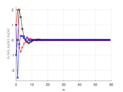
Figure 2: State trajectories of the nominal system (22), $x_{1}$ (black $\boldsymbol{\circ}$), $x_{2}$ (red  $\color[rgb]{1,0,0}\boldsymbol{\times}$), $x_{3}$ (blue $\color[rgb]{0,0,1}\boldsymbol{\square}$) with control input computed via Algorithm 11.

The case in which the control sequence computed by Algorithm 11 is applied to the perturbed system (26) is depicted by Figure 3. One clearly sees that the $x_{1}$-component, in which the perturbation enters in (26), is more strongly affected by the perturbation than the other components of the solution.

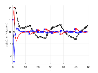
Figure 3: State trajectories of the perturbed system (26), $x_{1}$ (black $\boldsymbol{\circ}$), $x_{2}$ (red $\color[rgb]{1,0,0}~{}\boldsymbol{\times}$), $x_{3}$ (blue $\color[rgb]{0,0,1}\boldsymbol{\square}$) with control input computed via Algorithm 11.

Finally, Figure 4 illustrates the state trajectories associated with the shrinking horizon strategy with re-optimization, i.e., Algorithm 15 applied to the perturbed system (26). It may be observed that the re-optimization on shrinking horizons is able to mitigate the effect of the perturbation, as the maximal deviation of the $x_{1}$-component from the desired equilibrium $x_{1}=0$ after the transient phase is reduced by about 37%, from 0.615 to 0.387.

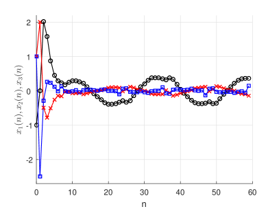
Figure 4: State trajectories of the perturbed system (26), $x_{1}$ (black $\boldsymbol{\circ}$), $x_{2}$ (red $\color[rgb]{1,0,0}\boldsymbol{\times}$), $x_{3}$ (blue $\color[rgb]{0,0,1}\boldsymbol{\square}$) with control input computed via Algorithm 15.

4.3 fs-CLF-based classic MPC

The shrinking horizon method is a rather unusual way of obtaining a feedback law via optimization based techniques. More commonly, one would use a classic MPC approach, in which the optimization is performed at every time step over a fixed horizon length $N$ and always the first element of the resulting control sequence is implemented. In this section we show that this approach can also be applied using fs-CLFs. To this end, we consider the following optimal control problem.

Problem 18.

Consider system (1) and let $M,N\in\mathbb{N}^{*}$. Let $\omega$ be a measurement function and $V$ be a fs-CLF with the associated decay function $\alpha\in\mathcal{K}_{\infty}$, $\alpha<\operatorname{id}$ be given. Also, let $x(0)=:\xi\in\mathcal{X}$. Compute ${\bf u}_{N}^{*}=\big{(}u_{0}^{*}(\xi),\ldots,u_{N-1}^{*}(\xi)\big{)}$ as the optimal solution of the following optimal control problem (OCP-3)

$$\begin{split}\min_{\textbf{u}_{N}}\,&\,\sum_{i=0}^{N-1}V\big{(}x(i,\xi,{\bf u}_{N})\big{)}\\ \mathrm{s.t.}&\,\mathrm{\,for\,all\,}j\in\{0,\dots,N-1\}\\ &\left\{\begin{array}[]{rcll}x(j+1)&=&g(x(j),u_{j})\\ u_{k}&\in&\mathcal{U}\\ g(x(j),u_{j})&\in&\mathcal{X}.\end{array}\right.\end{split}$$ (OCP-3)

Here we make use of the feedback signal at every time step. To do this, one can solve Problem 18 every single time-step and apply the first element of the corresponding optimal control sequence ${\bf u}_{N}$ to the system and then the (OCP-3) is solved again. This procedure is summarized by the following algorithm.

Algorithm 19.

At each time step $t\in\mathbb{N}$:

1. Measure the state $x(t)\in\mathcal{X}$ of system (1).

2. Set $\xi:=x(t)$, solve Problem 18 and denote the optimal control sequence satisfying (OCP-3) by ${\bf u}_{N}^{*}$.

3. Define the MPC-feedback value $\hat{q}_{\mathrm{MPC}}$ by

   $$\hat{q}_{\mathrm{MPC}}(\xi):=u_{0}^{*}(\xi)$$ (27)

   and apply it to system (1).

4. Go to Step 1.

The solution to the resulting MPC closed-loop system starting from some initial value $\xi$ and with optimization horizon $N$ is denoted by $x_{\mathrm{MPC}(N)}(\cdot,\xi)$. We denote the optimal value function related to Problem 18 by

$$V_{N}(\xi):=\sum_{i=0}^{N-1}V\big{(}x(i,\xi,{\bf u}_{N}^{*})\big{)}.$$ (28)

In order to analyze the resulting MPC closed-loop system, we make use of the following result.

Definition 20.

We say that the MPC scheme described in Algorithm 19 is semiglobally practically asymptotically $\omega$-stabilizing with respect to the optimization horizon $N$ in ${\cal A}:=\omega^{-1}(0)$, if there exists $\beta\in\mathcal{KL}$ such that the following property holds: for each $\delta>0$ and $\Delta>\delta$ there exists $N_{\delta,\Delta}\in\mathbb{N}^{*}$ such that for all optimization horizons $N\geq N_{\delta,\Delta}$ and all $\xi\in\mathbb{R}^{n}$ with $\omega(\xi)<\Delta$ the closed-loop solutions $x_{\mathrm{MPC}(N)}(\cdot,\xi)$ satisfy

$$\omega\big{(}x_{\mathrm{MPC}(N)}(t,\xi)\big{)}\leq\max\left\{\beta\big{(}\omega(\xi),t\big{)},\,\delta\right\}\qquad\forall t\in\mathbb{N}.$$

Proposition 21.

Let $\omega:\mathbb{R}^{n}\to\mathbb{R}_{\geq 0}$ be a measurement function and $V$ be a fs-CLF. Assume that there is a $\mathcal{K}_{\infty}$-function $\sigma$ such that the optimal value function $V_{N}$ from (28) satisfies

$$V_{N}(\xi)\leq\delta(V(\xi)),\quad\forall x\in\mathcal{X},N\in\mathbb{N}^{*}.$$

Then the MPC scheme obtained from Algorithm 19 is semiglobally practically asymptotically $\omega$-stabilizing in ${\cal A}:=\omega^{-1}(0)$ for system (1) with respect to the optimization horizon $N$. If, moreover, $\sigma$ is a linear function, i.e., $\sigma(r)=\gamma r$ for some $\gamma\in\mathbb{R}$, then the resulting MPC closed-loop is asymptotically $\omega$-stable in ${\cal A}:=\omega^{-1}(0)$ for all $N>2+\frac{\ln(\gamma-1)}{\ln\gamma-\ln(\gamma-1)}$.

Proof.

The first statement is proved by following similar arguments as those in [7, Theorem 6.37]. For the second statement, see [7, Corollary 6.21 and Remark 6.22]. We note that Theorem 6.37 and Corollary 6.21 in [7] consider stabilization at an equilibrium point. However, it is not hard to see that with the obvious modification of the arguments in these references we obtain that

$$V_{N}\big{(}x_{\mathrm{MPC}(N)}(t,\xi))\big{)}\leq\max\{\tilde{\beta}(V_{N}(\xi),i),\tilde{\delta}\}$$

for all $\xi$ with $V_{N}(\xi)\leq\widetilde{\Delta}$, $\widetilde{\Delta}>0$, $\tilde{\beta}\in\mathcal{KL}$, and $\tilde{\delta}\geq 0$, where $\widetilde{\Delta}\to\infty$ and $\tilde{\delta}\to 0$ as $N\to\infty$. Moreover, the inequality holds for arbitrarily large $\widetilde{\Delta}>0$ and $\tilde{\delta}=0$ if $\sigma$ is linear. Now, the inequalities

$$V(\xi)\leq V_{N}(\xi)\leq\delta(V(\xi)),$$

which follow by definition of $V_{N}$ and by the assumption of the proposition, imply that $V_{N}$ is a Lyapunov function for the closed loop, which proves (practical) asymptotic stability. ∎

In order to check whether the optimal value function (28) satisfies the conditions in Proposition 21, we make the following observation: From (7) and (3) it follows that there exists a $\mathcal{K}_{\infty}$-function $\hat{\kappa}$ such that for each admissible finite-step feedback control law $q:\mathcal{X}\to\mathcal{U}^{M}$ the inequality

$$V\Big{(}g^{i}\big{(}\xi,q_{1}(\xi),\ldots,q_{i}(\xi)\big{)}\Big{)}\leq\hat{\kappa}(V(\xi))$$ (29)

holds for all $i=1,\ldots,M-1$. This fact is easily verified for $\hat{\kappa}(r)=\max_{i=1,\ldots,M-1}\overline{\alpha}\circ\kappa_{i}\circ\underline{\alpha}^{-1}(r)$. Now we give the main result of this section.

Theorem 22.

Consider system (1) and let $M,N\in\mathbb{N}^{*}$. Let $\omega:\mathbb{R}^{n}\to\mathbb{R}_{\geq 0}$ be a measurement function and $V$ be a fs-CLF for the step size $M$. Then, the following statements hold.

1. If in (8) $\alpha(s)=cs$ with $c\in[0,1)$ and in (29) $\hat{\kappa}(r)=dr$ with $d>0$, then the MPC closed-loop is asymptotically $\omega$-stable with respect to the optimization horizon $N$ in ${\cal A}:=\omega^{-1}(0)$ for all $N>2+\frac{\ln(\gamma-1)}{\ln\gamma-\ln(\gamma-1)}$ with $\gamma=Md/(1-c)$.

2. If in (8) $\alpha(s)=cs$ with $c\in[0,1)$ and $\hat{\kappa}$ in (29) satisfies $\hat{\kappa}(r)\leq q\max\{r^{a},r^{b}\}$ for constants $a,b,q>0$, then the MPC scheme is semiglobally practically asymptotically $\omega$-stabilizing with respect to the optimization horizon $N$ in ${\cal A}$.

3. There exists $\rho\in\mathcal{K}_{\infty}$ such that if we replace $V$ by $\widetilde{V}=\rho(V)$ in Problem 18, then the MPC scheme is semiglobally practically asymptotically $\omega$-stabilizing with respect to the optimization horizon $N$ in ${\cal A}$.

Proof.

(i) Iterating (8) yields the existence of a control function ${\bf u}$ satisfying $V(x(kM,\xi,{\bf u}))\leq c^{k}V(\xi)$ and $V(x(kM+j,\xi,{\bf u}))\leq dV(x(kM,\xi,{\bf u}))$ for all $k\in\mathbb{N}$ and $j=0,\ldots,M-1$. Together this yields

$$V(x(kM+j,\xi,{\bf u}))\leq c^{k}dV(\xi),$$

which implies for $K\in\mathbb{N}$ such that $KM\geq N$

$$V_{N}(\xi) \leq \sum_{i=0}^{N-1}V\big{(}x(i,\xi,{\bf u})\big{)}$$

$$\leq \sum_{k=0}^{K-1}\sum_{j=0}^{M-1}V\big{(}x(kM+j,\xi,{\bf u})\big{)}$$

$$\leq \sum_{k=0}^{K-1}Mc^{k}dV(\xi)\;\leq\;\frac{Md}{1-c}V(\xi).$$

Now the second part of Proposition 21 with $\delta(r)=\frac{Md}{1-c}r$ yields the claim.

(ii) Iterating (8), as in (i) we obtain the inequality

$$\begin{split}V(x(kM+j,\xi,{\bf u}))&\leq q\max\{(c^{k}V(\xi))^{a},(c^{k}V(\xi))^{b}\}\\ &\leq q\max\{c^{a},c^{b}\}^{k}\max\{V(\xi)^{a},V(\xi)^{b}\}.\end{split}$$

Abbreviating $\hat{c}=\max\{c^{a},c^{b}\}\in[0,1)$ the same computation as in (i) yields

$$\begin{split}V_{N}(\xi)&\leq\sum_{k=0}^{K-1}Mq\hat{c}^{k}\max\{V(\xi)^{a},V(\xi)^{b}\}\\ &\leq\frac{Mq}{1-\hat{c}}\max\{V(\xi)^{a},V(\xi)^{b}\}.\end{split}$$

This implies that the assumptions of the first part of Proposition 21 are satisfied with $\delta(r)=\frac{Mq}{1-\hat{c}}\max\{r^{a},r^{b}\}$ and the claim follows.

(iii) Recall $\hat{\kappa}$ from (29). From (8) it follows that

$$\hat{\kappa}(V(x(M,\xi,{\bf u}_{q})))\leq\hat{\kappa}\circ\alpha(V(\xi))=\underbrace{\hat{\kappa}\circ\alpha\circ\hat{\kappa}^{-1}}_{=:\mu}(\hat{\kappa}(V(\xi)).$$

Since $\alpha<\operatorname{id}$ it follows that $\mu<\operatorname{id}$. Hence, applying Proposition 3.2 from [27] to $\widehat{V}=\hat{\kappa}(V)$ implies that there exists $\rho\in\mathcal{K}_{\infty}$ and $\lambda\in(0,1)$ such that $W:=\rho(\widehat{V})$ satisfies $W(x(M,\xi,{\bf u}_{q}))\leq\lambda W(\xi)$. Iterating this inequality yields the existence of ${\bf u}$ with

$$\begin{split}W(x(kM,\xi,{\bf u}))\leq\lambda^{k}W(\xi)\\ V(x(kM+j,\xi,{\bf u}))\leq\hat{\kappa}(V(x(kM,\xi,{\bf u}))).\end{split}$$

For $\widetilde{V}=\rho(V)$ this implies

$$\begin{split}\widetilde{V}(x(kM+j,\xi,{\bf u}))&=\rho(V(x(kM+j,\xi,{\bf u}))\\ &\leq\rho\circ\hat{\kappa}(V(x(kM,\xi,{\bf u}))\\ &=W(x(kM,\xi,{\bf u}))\\ &\leq\lambda^{k}W(\xi)=\lambda^{k}\underbrace{\rho\circ\hat{\kappa}\circ\rho^{-1}}_{=:\sigma\in\mathcal{K}_{\infty}}(\widetilde{V}(\xi)).\end{split}$$

With an analogous computation as in (i) and (ii) we obtain

$$\begin{split}V_{N}(\xi)\leq\sum_{k=0}^{K-1}\sum_{j=0}^{M-1}\widetilde{V}\big{(}x(kM+j,\xi,{\bf u})\big{)}\\ \hskip 28.45274pt\leq\sum_{k=0}^{K-1}M\lambda^{k}\sigma(\widetilde{V}(\xi))\leq\frac{M}{1-\lambda}\sigma(\widetilde{V}(\xi)).\end{split}$$

Hence, the assumptions of the first part of Proposition 21 are satisfied for $\widetilde{V}$ in place of $V$ with $\delta(r)=M\sigma(r)/(1-\lambda)$. Thus, Proposition 21 yields the assertion. ∎

Example 23.

We illustrate the performance of the classic MPC approach again for the nominal and perturbed systems (22) and (26). We use the same initial condition $\xi=(-1,1,1)^{T}$ as in Example 17, the fs-CLF $V(x)=x^{T}Px$ from Example 17 as stage cost and the optimization horizon $N=6$. Figure 5 shows the resulting state trajectory for applying the control computed by Algorithm 19 to the perturbed system (26). The effect of the perturbation is comparable to the updated shrinking horizon MPC Algorithm in Figure 4; after the transient phase the maximal deviation of $x_{1}$ to the desired equilibrium is 0.363 here compared to 0.387 in the shrinking horizon algorithm. However, one observes that the trajectories in Figure 5 appear smoother than those in Figure 4. Further numerical tests have revealed that the loss of smoothness in Figure 4 is mainly due to the contractive constraints and not due to the shrinking horizon. Hence, this is an advantage for MPC without using contraction constraints. However, we emphasize that we have not rigorously checked the assumptions of Theorem 22 (which are usually quite conservative, anyway), but rather determined the optimization horizon $N$ by trial and error. Hence, in contrast to Algorithms 11 and 15, there is no formal guarantee for asymptotic stability here.

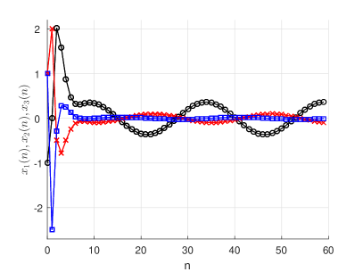
Figure 5: State trajectories of the perturbed system (26), $x_{1}$ (black $\boldsymbol{\circ}$), $x_{2}$ (red $\color[rgb]{1,0,0}\boldsymbol{\times}$), $x_{3}$ (blue $\color[rgb]{0,0,1}\boldsymbol{\square}$) with control input computed via Algorithm 19.

5 Conclusions and outlook

We have exploited the notion of fs-CLF to develop control design approaches for discrete-time systems. To this end, the controller design problem has been reformulated into an optimization problem. Motivated by state-of-the-art applications, we have provided three different MPC schemes via fs-CLFs: i) contractive multi-step MPC, ii) contractive updated multi-step MPC, iii) classic MPC without stabilizing terminal constraints. We have illustrated the MPC schemes via an example.

The results of the paper can be extended in several directions: fs-LFs are leveraged to develop nonconservative small-gain and dissipativity conditions for stability analysis of large-scale systems [28, 3, 4, 6]. We aim to fuse the results of the current paper with the nonconservative small-gain and dissipativity to develop distributed MPC schemes. Applications of such results to smart grids, smart city and mobile robots are expected. The analysis in this work can also be generalized to systems subject to disturbances.

References

- [1] H. K. Khalil, Nonlinear systems, 3rd ed. Englewood Cliffs, NJ: Prentice-Hall, 2002.
- [2] R. Geiselhart, R. H. Gielen, M. Lazar, and F. R. Wirth, “An alternative converse Lyapunov theorem for discrete-time systems,” Syst. Control Lett., vol. 70, pp. 49–59, 2014.
- [3] R. Geiselhart, M. Lazar, and F. R. Wirth, “A relaxed small-gain theorem for interconnected discrete-time systems,” IEEE Trans. Autom. Control, vol. 60, no. 3, pp. 812–817, 2015.
- [4] R. H. Gielen and M. Lazar, “On stability analysis methods for large-scale discrete-time systems,” Automatica, vol. 55, pp. 66–72, 2015.
- [5] R. Geiselhart and F. R. Wirth, “Relaxed ISS small-gain theorems for discrete-time systems,” SIAM J. Control Optim., vol. 54, no. 2, pp. 423–449, 2016.
- [6] N. Noroozi, R. Geiselhart, L. Grüne, B. S. Rüffer, and F. R. Wirth, “Nonconservative discrete-time ISS small-gain conditions for closed sets,” IEEE Trans. Autom. Control, vol. 63, no. 5, pp. 1231–1242, 2018.
- [7] L. Grüne and J. Pannek, Nonlinear Model Predictive Control: Theory and Algorithms, 2nd ed. London: Springer, 2017.
- [8] P. Varutti and R. Findeisen, “Compensating network delays and information loss by predictive control methods,” in Eur. Control Conf., Budapest, Aug 2009, pp. 1722–1727.
- [9] L. Grüne, J. Pannek, and K. Worthmann, “A prediction based control scheme for networked systems with delays and packet dropouts,” in 48h IEEE Conf. Decision Control, Shanghai, Dec 2009, pp. 537–542.
- [10] L. Grüne and V. G. Palma, “Robustness of performance and stability for multistep and updated multistep MPC schemes,” Discrete Continuous Dyn. Syst. - A, vol. 35, p. 4385, 2015.
- [11] L. Grüne and M. Sigurani, “A Lyapunov based nonlinear small-gain theorem for discontinuous discrete-time large-scale systems,” in Proc. 21st Int. Symp. Mathematical Theory Networks Syst., 2014, pp. 439–446.
- [12] M. Alamir, “Contraction-based nonlinear model predictive control formulation without stability-related terminal constraints,” Automatica, vol. 75, pp. 288–292, 2017.
- [13] S. L. de Oliveira Kothare and M. Morari, “Contractive model predictive control for constrained nonlinear systems,” IEEE Trans. Autom. Control, vol. 45, no. 6, pp. 1053–1071, 2000.
- [14] J. Wan, “Computationally reliable approaches of contractive MPC for discrete-time systems,” Ph.D. dissertation, University of Girona, Girona, 2007.
- [15] T. H. Yang and E. Polak, “Moving horizon control of nonlinear systems with input saturation, disturbances and plant uncertainty,” Int. J. Control, vol. 58, no. 4, pp. 875–903, 1993.
- [16] K. Worthmann, “Stability Analysis of Unconstrained Receding Horizon Control Schemes,” PhD Thesis, Universität Bayreuth, 2011.
- [17] J. Hanema, M. Lazar, and R. Tóth, “Stabilizing tube-based model predictive control: Terminal set and cost construction for LPV systems,” Automatica, vol. 85, pp. 137–144, 2017.
- [18] M. Lazar and V. Spinu, “Finite-step terminal ingredients for stabilizing model predictive control,” in 5th IFAC Conf. Nonlinear Model Predictive Control, Seville, Spain, Sep 2015, pp. 9–15.
- [19] L. Grüne, “Analysis and design of unconstrained nonlinear MPC schemes for finite and infinite dimensional systems,” SIAM J. Control Optim., vol. 48, pp. 1206–1228, 2009.
- [20] L. Grüne, J. Pannek, M. Seehafer, and K. Worthmann, “Analysis of unconstrained nonlinear MPC schemes with time varying control horizon,” SIAM J. Control Optim., vol. 48, pp. 4938–4962, 2010.
- [21] G. Grimm, M. J. Messina, S. E. Tuna, and A. R. Teel, “Model predictive control: for want of a local control Lyapunov function, all is not lost,” IEEE Trans. Autom. Control, vol. 50, no. 5, pp. 546–558, 2005.
- [22] S. E. Tuna, M. J. Messina, and A. R. Teel, “Shorter horizons for model predictive control,” in Amer. Control Conf., Minneapolis, 2006, pp. 863–868.
- [23] L. Grüne and A. Rantzer, “On the infinite horizon performance of receding horizon controllers,” IEEE Trans. Automat. Control, vol. 53, pp. 2100–2111, 2008.
- [24] C. M. Kellett, “A compendium of comparison function results,” Math. Control Signals Syst., vol. 26, no. 3, pp. 339–374, 2014.
- [25] R. Geiselhart and N. Noroozi, “Equivalent types of ISS Lyapunov functions for discontinuous discrete-time systems,” Automatica, vol. 84, pp. 227–231, 2017.
- [26] R. Geiselhart and F. Wirth, “Solving iterative functional equations for a class of piecewise linear -functions,” J. Math. Anal. Appl., vol. 411, no. 2, pp. 652 – 664, 2014.
- [27] L. Grüne and C. M. Kellett, “ISS-Lyapunov functions for discontinuous discrete-time systems,” IEEE Trans. Autom. Control, vol. 59, no. 11, pp. 3098–3103, 2014.
- [28] N. Noroozi and B. S. Rüffer, “Non-conservative dissipativity and small-gain theory for ISS networks,” in 53rd IEEE Conf. Decision Control, Los Angeles, 2014, pp. 3131–3136.