Preventing the Generation of Inconsistent Sets of Classification Rules

Abstract

In recent years, the interest in interpretable classification models has grown. One of the proposed ways to improve the interpretability of a rule-based classification model is to use sets (unordered collections) of rules, instead of lists (ordered collections) of rules. One of the problems associated with sets is that multiple rules may cover a single instance, but predict different classes for it, thus requiring a conflict resolution strategy. In this work, we propose two algorithms capable of finding feature-space regions inside which any created rule would be consistent with the already existing rules, preventing inconsistencies from arising. Our algorithms do not generate classification models, but are instead meant to enhance algorithms that do so, such as Learning Classifier Systems. Both algorithms are described and analyzed exclusively from a theoretical perspective, since we have not modified a model-generating algorithm to incorporate our proposed solutions yet. This work presents the novelty of using conflict avoidance strategies instead of conflict resolution strategies.

I Introduction

Classification is one of the commonest tasks of Machine Learning, concisely described in [1] as the generation of a model that learns relations between predictive features and target features. This learning occurs by adjusting the internal parameters of the model.

In recent years, the interest in interpretable classification models has grown, partly due to regulations such as the General Data Protection Regulation (commonly known as GDPR), that created a “right to explanation”, a regulation “whereby a user can ask for an explanation of an algorithmic decision that significantly affects them” [2].

Even though interpretability, in the context of classification models, is not an objectively and consistently defined concept [3], it is reasonable to say that some types of classification models are inherently more interpretable than others; a Decision Tree [4], for instance, can be said to be more interpretable than a Deep Neural Network [5].

It is generally accepted that rule-based classifiers are among the most interpretable [6]. The training phase of such classifiers usually consist in creating and tuning a list of classification rules. A classification rule usually has two components, its antecedent and its consequent. The antecedent is a collection of tests over feature values, and the consequent is the label that will be assigned to the dataset instance which will be classified, if it passes all the antecedent’s tests. A simple classification rule is exemplified in Figure 1.

Figure 1: Simple Classification Rule

The interpretability of a rule-based classification model is frequently measured by its size, i.e. the number of rules in the model and/or the number of features tested by the rules [6]. Therefore, many algorithms that generate interpretable classification models try to minimize the model size.

In [1], however, the authors propose an alternative way of improving the interpretability of a rule-based classification model, using sets (unordered collections) of rules, instead of lists (ordered collections).

If a classifier employs a list of rules, then its n-th rule cannot be correctly interpreted alone, because an instance that is covered by it may also be covered by a previous rule; the actual class predicted by the classifier would be the one of the previous rule. Using, instead, a set of rules allows the user to analyze the rules individually, making the model more interpretable.

However, using a set of rules may create conflicts when multiple rules (with different consequents) cover the same dataset instance. The authors of [1] discuss two conflict resolution strategies, allowing the classifier to function properly even if it contains multiple rules that contradict each other.

In this work, we propose two algorithms capable of finding sets of feature-space regions such that any rule created within those regions will always be consistent with $R$. In this context, a rule $r_{1}$ is said to be consistent with a rule $r_{2}$ if their consequents are identical or if there is no intersection between their antecedents, i.e. it is not possible to create an object that would be covered by rules that predict different labels. A set of rules is said to be consistent if each rule of the set is consistent with each other.

By only creating consistent rules, one avoids the problem of conflicting predictions entirely, hence improving the interpretability of the classification model.

The proposed algorithms do not generate classification models by themselves, instead they are meant to enhance algorithms that do so. They can be used, for instance, during the initialization and mutation phases of a genetic algorithm. Since no model is directly generated, our algorithms can only be evaluated by modifying an existing model-building algorithm to use one of the methods, then measuring the relative change on the induced models. The two algorithms themselves are independent of the metrics chosen.

It is interesting to note that our algorithms are not sensitive to the type of the consequent of the rules, as long as they can be tested for equality. This means that they can be used to supplement algorithms that generate any kind of rule format, since inconsistencies between rules arise from overlaps between the rules’ antecedents.

The remainder of this work is organized as follows: in Section II we discuss related works; in Section III we present two algorithms to aid the creation of consistent rules, and analyze their properties; in Section IV we discuss future works and present our conclusions.

II Related Works

The concept of interpretability has been a point of contention in Artificial Intelligence (AI) literature. There are many different views on what constitute an interpretable classification model, how to measure interpretability, and whether it is necessary to, or even worth to, sacrifice predictive power of a classifier in favor of its interpretability. Some authors have proposed mechanisms to improve the interpretability of black-box models [7], while other have focused on transparent rule-based models, such as Learning Classifier Systems [8]. In this section, we will discuss some of the works which have focused on algorithms that generate rule-based models, and why interpretability is important.

In [9] and [10] the authors argue that AI models do not usually operate in a vacuum, they interact with humans, and that various types of Human-AI interactions may benefit from an interpretable model.

In areas such as bioinformatics (protein function prediction, gene function prediction, among others) it is important that the classification model is interpretable, in order to make it possible for its users to validate it [11]. In medical and financial applications, understanding a computer-induced model is often a prerequisite for users to trust the model’s predictions [6].

Considering that rule-based classification models are inherently transparent, thus interpretable, many algorithms that generate interpretable models have been published (see the discussion of transparency in [3]).

The Decision Tree algorithm C4.5 [12], for instance, generates models that can be interpreted as easily as a flowchart. It also employs a pruning strategy that improves simultaneously the interpretability of the model, by reducing its size, and its predictive power, by reducing overfitting.

In [13], the authors modified the algorithm C4.5 to handle multi-label classification. One of the most interesting parts of their work, from an interpretability perspective, was the generation of a set of rules from the decision tree. This process of “splitting” a decision tree into a set of rules is one of the few processes that we know of that can generate a consistent set of rules.

In [14], the authors propose an algorithm based on Predictive Clustering Trees (PCTs) [15] to perform hierarchical multi-label classification using a single, global model. PCT-based algorithms see decision trees as hierarchies of clusters and as such, during the model training phase, they try to minimize intra-cluster variance. The proposed algorithm, called Clus-HMC, was later modified in [16] to handle class hierarchies organized as Directed Acyclic Graphs (DAGs), and used in [17] to generate a collection of trees which build an ensemble.

In [18], the authors propose an evolutionary algorithm to generate interpretable fuzzy classification rules by using the Pittsburg approach, in which each individual of the population represents a complete classifier. The fittest selection mechanism used was the multi-objective algorithm NSGA-2 [19], and the functions being optimized were accuracy, number of rules, and length of rules. The authors also discuss the issue of interpretability of fuzzy classification rules and strategies to improve it, such as merging similar fuzzy sets.

In [20], the authors propose a Genetic Algorithm (GA) to generate interpretable traditional (non-fuzzy) classification rules. The algorithm, called HMC-GA, is the only GA-based method in the literature that is capable of building a global hierarchical multi-label classification model [21].

In [22], the authors propose the first ant colony-based classification algorithm, called Ant-Miner. It generates lists of classification rules, and had, in its original version, the limitation of only handling categorical features. Ant-Miner was used as a base for many algorithms, such as Multi-Label Ant-Miner (MuLAM) [23], which generates flat (i.e. non-hierarchical) multi-label classification rules; cAnt-Miner [24], which removed the restriction of using only categorical features; h-Ant-Miner [25], which generates hierarchical single-label classification rules; and hm-Ant-Miner [11], which generates hierarchical multi-label classification rules.

In [26], the authors propose a new sequential covering strategy for cAnt-Miner, in an algorithm called cAnt-Miner${}_{\text{pb}}$. This algorithm was later enhanced to generate sets (unordered collections) of rules in an algorithm called Unordered cAnt-Miner${}_{\text{pb}}$ [1]. The authors of Unordered cAnt-Miner${}_{\text{pb}}$ argue that a set of rules is more interpretable than a list (ordered collection) of rules. They also propose a new interpretability metric, called Prediction-Explanation Size, that accounts for the inter-dependency of rules in lists.

The sets of rules generated by Unordered cAnt-Miner${}_{\text{pb}}$ could contain inconsistent rules, i.e. multiple rules that cover the same dataset instance but predict different classes for it. The authors discuss mechanisms to resolve such conflicts when they arise (i.e. when making a prediction), such as using the rule with the highest quality, or aggregating the predictions of the conflicting rules and selecting the most common label in the aggregation.

The idea that sets of rules are more interpretable than lists of rules, and the fact that there are, as far as we are aware, no mechanisms to prevent the generation of inconsistent rules, motivated us to research and develop the algorithms described in Section III.

III Proposed Algorithms

We propose two algorithms to solve the problem of adding a new rule to an existing set of consistent rules, creating an expanded rule set that is still consistent. More specifically, the algorithms find feature-space regions in which rules can be created while being consistent with an already existing set of rules; the actual creation of the rules inside such regions is not within the scope of the methods.

There is a important distinction between identifying if a new rule is consistent with an existing collection of rules and creating a new rule that is consistent with an existing collection of rules; the first task, analogous to determining if a cake tastes good, is trivial; the second task, analogous to baking a good cake, is far more complex. The algorithms we propose are meant to guide the execution of the later task.

To the best of our knowledge, both algorithms, and the conflict avoidance approach they employ, are new to the literature. We refer to these algorithms as Constrained Feature-Space Greedy Search (CFSGS) and Constrained Feature-Space Box-Enlargement (CFSBE). We present them, respectively, in Section III-A and Section III-B.

Whenever we refer to a rule, unless stated otherwise, we will be referring only to its antecedent. The case in which rules have the same consequent but different antecedents, hence are consistent with each other, will be discussed in Section III-D.

We will assume that all predictive features are continuous. Both algorithms can handle categorical features, but explaining them exclusively in terms of continuous features allows a better visualization and explanation. We will discuss the treatment of categorical features in Section III-C.

In order to simplify the explanation of both algorithms we will use the convention that rules have exactly one feature test for each predictive feature and have the format shown in Equation 1, where $test_{i}$ denotes the i-th test of the rule, i.e. the test over the i-th feature, and $|f|$ denotes the number of features in the dataset. We will also use the convention that feature tests have the format shown in Equation 2, where $f_{i}$ denotes the value of the i-th feature of the dataset instance being tested, and $test.lower$ and $test.upper$ are, respectively, the lower and upper bound values of the test.

$$\begin{split}rule:=test_{1}\wedge test_{2}\wedge\dots\wedge test_{|f|}\end{split}$$ (1)

$$\begin{split}test:=test.lower\leq f_{i}<test.upper\end{split}$$ (2)

It is important to observe that the lower bound of a test is inclusive, but the upper bound is exclusive. This definition prevents inconsistencies when two tests from different rules “touch” each other, i.e. the upper bound of the i-th test from a rule has the same value as the lower bound of the i-th test from another rule. To exemplify this, consider the rules described in Equations 3 and 4. If we use an inclusive upper bound, a person with $age=10$ will be covered by both rules, which will make the rules inconsistent with each other.

$$rule_{1}=\textbf{IF } 0\leq age<10 \textbf{ THEN }class=child$$ (3)

$$rule_{2}=\textbf{IF } 10\leq age<99 \textbf{THEN }class=adult$$ (4)

Both algorithms can be more easily explained if we use a geometric interpretation, that is, by viewing the antecedent of a classification rule as an $|f|$-dimensional hyperrectangle, being $f$ the set of features of the dataset.

Figure 2 shows what three classification rules, represented as colored rectangles, and seven dataset instances, represented as black dots, could look like in a classification problem with two predictive features, $f_{1}$ and $f_{2}$.

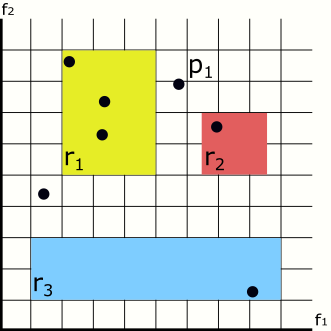
Figure 2: Classification rules in 2D feature-space

Considering that the grid squares in Figure 2 have unitary length, the antecedent of the rules depicted in the figure can be formally described by Equations 5, 6 and 7.

$$\begin{split}rule_{1}=\begin{cases}test_{1}=2\leq f_{1}<5\\ test_{2}=5\leq f_{2}<9\end{cases}\end{split}$$ (5)

$$\begin{split}rule_{2}=\begin{cases}test_{1}=6.5\leq f_{1}<8.5\\ test_{2}=5\leq f_{2}<7\end{cases}\end{split}$$ (6)

$$\begin{split}rule_{3}=\begin{cases}test_{1}=1\leq f_{1}<9\\ test_{2}=1\leq f_{2}<3\end{cases}\end{split}$$ (7)

The premise of the two proposed algorithms is that if we can find a region of the feature-space that is not covered by any rule, we could create a rule inside such region. The new rule would be consistent with the already existing rules, because no dataset instance could be simultaneously covered by more than one rule.

III-A Constrained Feature-Space Greedy Search

Since the region covered by a rule is the region described by the conjunction of its tests, the region not covered by it can be described by the the disjunction of the negation of its tests, as we can see in Equations 8 and 9.

$$rule =test_{1}\wedge\dots\wedge test_{n}$$ (8)

$$\lnot rule =\lnot(test_{1}\wedge\dots\wedge test_{n})$$

$$\lnot rule =(\lnot test_{1})\lor\dots\lor(\lnot test_{n})$$

$$test_{i} =lower_{i}\leq f_{i}<upper_{i}$$ (9)

$$test_{i} =(lower_{i}\leq f_{i})\land(f_{i}<upper_{i})$$

$$\lnot test_{i} =\lnot((lower_{i}\leq f_{i})\land(f_{i}<upper_{i}))$$

$$\lnot test_{i} =\lnot(lower_{i}\leq f_{i})\lor\lnot(f_{i}<upper_{i})$$

$$\lnot test_{i} =(lower_{i}>f_{i})\lor(f_{i}\geq upper_{i})$$

$$\lnot test_{i} =(f_{i}<lower_{i})\lor(f_{i}\geq upper_{i})$$

Negating the tests of $r_{1}$, for instance, results in four inequalities (or constraints), each describing a region not covered by the rule:

• $f_{1}<2$ , the region to the left of the yellow rectangle

• $f_{1}\geq 5$ , the region to the right of the yellow rectangle

• $f_{2}<5$ , the region below the yellow rectangle

• $f_{2}\geq 9$ , the region above the yellow rectangle

In Constrained Feature-Space Greedy Search (CFSGS), we create a collection $C$ with the constraints generated by the negation of all the tests from all the rules, with $C_{i,j}$ denoting the j-th inequality generated from the i-th rule. The constraints generated from the negation of the tests of $r_{1}$, $r_{2}$, and $r_{3}$ are shown in Table II. As we assumed that all features are continuous, the number of constraints generated per rule, $n_{f}$, is equal to $2\cdot|f|$. We discuss the relation between $n_{f}$ and the data type of the features (categorical or continuous) in Section III-C.

TABLE I: Constraints Generated From Rules

TABLE II: Constraints Generated From Rules

Index in $C$	Constraint Generated
$C_{1,1}$	$f_{1}<2$
$C_{1,2}$	$f_{1}\geq 5$
$C_{1,3}$	$f_{2}<5$
$C_{1,4}$	$f_{2}\geq 9$
$C_{2,1}$	$f_{1}<6.5$
$C_{2,2}$	$f_{1}\geq 8.5$
$C_{2,3}$	$f_{2}<5$
$C_{2,4}$	$f_{2}\geq 7$
$C_{3,1}$	$f_{1}<1$
$C_{3,2}$	$f_{1}\geq 9$
$C_{3,3}$	$f_{2}<1$
$C_{3,4}$	$f_{2}\geq 3$

By using Algorithm 1 we can organize $C$ into a Directed Acyclic Graph (DAG). Doing so allows us to perform a greedy search to find all subsets of $C$ that contain exactly one constraint from each rule and all constraints are simultaneously satisfiable. Such subsets of $C$ describe non-empty regions of the feature-space that are not covered by any rule. The DAG generated from the constraints of $r_{1}$, $r_{2}$, and $r_{3}$ is shown in Figure 3.

Algorithm 1 CFSGS - DAG Build

1:

2:Collection of constraints: $C$

3:Number of existing rules: $n_{r}$

4:Number of constraints generated from a rule: $n_{f}$ (number of categorical features plus 2 times the number of continuous features)

5:

6:The DAG $G$ representing the constrained feature-space to be explored

7:

8:G $\leftarrow$  New Directed Graph

9:$G.E\leftarrow\{\}$ $\triangleright$ The set of edges of G

10:$G.V\leftarrow\{root\}$ $\triangleright$ The set of vertices of G

11:for $i\in\{1,2,\ldots,n_{r}\}$ do

12:    for $j\in\{1,2,\ldots,n_{f}\}$ do

13:         $G.V\leftarrow G.V\cup\{{C_{i,j}}$}

14:         if $i>1$ then

15:             for $k\in\{1,2,\ldots,n_{f}\}$ do

16:                 $G.E\leftarrow G.E\cup\{(C_{i-1,k},C_{i,j})\}$

17:             end for

18:         end if

19:    end for

20:end for

21:return $G$

Figure 3: Constraints as DAG

The objective of the search is to find consistent paths from the root to a leaf node. A path is said to be consistent iff the constraints represented by its nodes can all be simultaneously satisfied, such as the one described in Equation 10. If adding a node to the path currently being explored makes the constraints unsatisfiable, the search algorithm backtracks and tries adding another node.

$$\{C_{1,1},C_{2,1},C_{3,1}\} =(f_{1}<2)\wedge(f_{1}<6.5)\wedge(f_{1}<1)$$ (10)

$$=f_{1}<1$$

We could fully explore the DAG to generate all consistent paths, but since we only need one, we stop the search as soon as the first one is found. It is important to observe that the order in which the nodes within a level are explored determine the order in which paths are found. If the nodes are explored in a lexicographic order, e.g. $C_{1,1}$ is explored before $C_{1,2}$, the first paths found will have a bias for the lower regions of the first features (e.g. bottom left area in Figure 2). To remove this bias, it suffices to explore the nodes of each level in a random order.

The runtime complexity of building the DAG can be expressed in function of the number of existing rules $n_{r}$ and the number of constraints generated per rule $n_{f}$.

In Algorithm 1, line 7 is executed $n_{r}\cdot n_{f}$ times, due to the two nested loops. Line 10 is executed $n_{r}\cdot(n_{f}-1)\cdot n_{f}$ times, since the conditional in line 8 decreases the number of iterations by one. Considering the cost of line 7 to be a constant $k_{1}$, and the cost of the line 10 to be a constant $k_{2}$, the total cost of building the DAG is described by Equation 11.

$$T(n_{f},n_{r}) =n_{r}\cdot n_{f}\cdot k_{1}+n_{r}\cdot(n_{f}-1)\cdot n_{f}\cdot k_{2}$$ (11)

$$T(n_{f},n_{r}) \in\mathcal{O}(n_{f}^{\text{\hskip 4.2679pt2}}\text{\hskip 2.84526pt}\cdot n_{r})$$

For the search algorithm, the worst-case scenario of having no possible consistent paths would cause the exploration of every path. Since creating a path is choosing an edge, out of $n_{f}$ edges, repeated over $n_{r}$ levels of the graph, there are exactly $n_{f}^{\text{\hskip 4.2679pt}n_{r}}$ possible paths, leading to a complexity cost of $\mathcal{O}(n_{f}^{\text{\hskip 4.2679pt}n_{r}})$.

The total computational cost of CFSGS is the sum of building the DAG and exploring it, which makes the method bounded by $(\mathcal{O}(n_{f}^{\text{\hskip 4.2679pt2}}\text{\hskip 2.84526pt}\cdot n_{r})+\mathcal{O}(n_{f}^{\text{\hskip 4.2679pt}n_{r}}))\in\mathcal{O}(n_{f}^{\text{\hskip 4.2679pt}n_{r}})$. While the algorithm is capable of finding all sub-regions where a consistent rule could be created, this exponential complexity cost makes it unsuitable for many applications.

III-B Constrained Feature-Space Box-Enlargement

Extending the geometrical interpretation provided by CFSGS, we would like a way to guide the search through the DAG such that the cost becomes polynomial in relation to the number of features and rules. Constrained Feature-Space Box-Enlargement’s central idea is that it is possible to leverage information from the training dataset to visit only nodes that lead to a possible consistent path to a leaf node.

Instead of searching the feature-space for suitable regions, CFSBE starts from a point known not to be covered by any rule, called a “seed”, and “enlarge” this point along the different dimensions, creating a box that does not overlap with any of the existing rules’ antecedents. A rule created inside such box would also not overlap with the existing rules, so they would be consistent, regardless of their consequent.

Searching for arbitrary non-covered points is equivalent to searching for non-covered regions, being as computationally expensive as CFSGS. However, if we keep track of which dataset instances are not covered by any rules we may use one of such instances as the seed. By using an associative array structure to map which points are covered by which rules, choosing a seed would have cost $\mathcal{O}(1)$, and updating the structure on the insertion or removal of a rule would have cost $\mathcal{O}(n)$, $n$ being the number of instances in the training dataset.

After selecting a non-covered point as seed, we must choose the order in which the dimensions will be expanded. Consider the point $p_{1}$ in Figure 2; if we first enlarge it along the $f_{1}$ dimension and $f_{2}$ afterwards, we end up with the green region shown in Figure 4. If, however, we start with $f_{2}$, we end up with the green region shown in Figure 5.

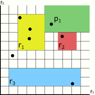
Figure 4: CFSBE - Horizontal Axis First

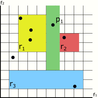
Figure 5: CFSBE - Horizontal Axis First

Once a seed point and a feature order is chosen, a degenerate hyperrectangle (or box) is created around the point. The box is then enlarged in each dimension according to the chosen ordering.

To determine the limit of the expansion along each dimension, that is, the boundaries to which the box can grow without overlapping with existing rules, it is necessary to check which rules “intersect” with the box on the other dimensions.

To exemplify the need for checking for “intersections” on dimensions that are not currently being expanded on, consider the point $p_{1}$ in Figure 2. Even though it is not covered by any rule, it does pass the $f_{2}$ feature test of the rule $r_{1}$, i.e. it “intersects” the rule $r_{1}$ on the $f_{2}$ dimension. If we create our box around $p_{1}$ and grow it along the $f_{1}$ dimension, it would eventually contain points that satisfy both tests of $r_{1}$, i.e. there would be an intersection between the box and $r_{1}$.

The method used to safely grow a box in such a way that it does not overlap with the boxes described by the antecedents of a set of rules is presented in Algorithm 2.

Algorithm 2 Constrained Feature-Space Box-Enlargement

1:

2:Set of non-overlapping rules $R$

3:Seed point $x$, not covered by any rule of $R$

4:Order of dimensions to expand $O_{d}$ (a permutation of $\{1,2,\ldots,|O_{d}|\}$)

5:

6:The box $B$ covers a possible hyperrectangle containing $x$ that can not be further expanded, and does not intersect any rule of R

7:

8:$B\leftarrow$  Degenerate rectangle with $|O_{d}|$ dimensions

9:for $i\in O_{d}$ do

10:    $B_{i}.lower\leftarrow x_{i}$

11:    $B_{i}.upper\leftarrow x_{i}$

12:end for

13:for $d\in O_{d}$ do

14:    $B_{d}.lower\leftarrow-\infty$

15:    $B_{d}.upper\leftarrow+\infty$

16:    for $r\in R$ do

17:         if $Intersects(B,r,d)$ then

18:             if $x_{d}\geq r_{d}.upper$ then

19:                 $B_{d}.lower\leftarrow max(B_{d}.lower,~{}r_{d}.upper)$

20:             else$\triangleright$ Meaning $x_{d}<r_{d}.lower$, otherwise $x$ would be covered by $r$

21:                 $B_{d}.upper\leftarrow min(B_{d}.upper,~{}r_{d}.lower)$

22:             end if

23:         end if

24:    end for

25:end for

26:return $B$

27:

28:function Intersects(Box B, Rule r, Dimension to skip d)

29:    $NumDimensions\leftarrow\lvert r\rvert$

30:    for $i\in\{1,2,\ldots,NumDimensions\}\setminus d$  do

31:         $u\leftarrow B_{i}.upper>r_{i}.lower$

32:         $l\leftarrow B_{i}.lower<r_{i}.upper$

33:         if $\lnot(u\land l)$ then

34:             return False

35:         end if

36:    end for

37:    return True

38:end function

It is worth noting that even though CFSBE cannot find all suitable hyperrectangles, it can find all the arguably relevant ones. Consider the dataset depicted in Figure 2, CFSGS could find a region below the blue rectangle, while CFSBE cannot; but since there are no instances there, it is arguable that the rules created in such region would not be useful, as their coverage would be zero and their predictive power could not be measured on the dataset used to train the classification model.

CFSBE’s runtime complexity can be calculated in a straightforward manner. Let $d$ be the number of dimensions (features) in the dataset and $r$ be the number of rules in the set of existing rules. The innermost part of the algorithm, in lines 11 through 15, has a constant cost, $k_{1}$, because they do not depend on the values of $d$ or $r$. The $Intersects$ function has a loop that executes at most $d-1$ steps. The contents of this loop do not depend on $d$ nor $r$, therefore they also have a constant cost, $k_{2}$, hence the worst-case scenario for this function is $T_{1}(d)=(d-1)\cdot k_{2}$.

Lines 1 through 4 perform the initialization of the degenerated rectangle, which occurs in a loop with $d$ steps, each step having constant cost $k_{3}$. The rest of the algorithm is a trivial nesting of loops, the first of which takes $d$ steps, the second $r$ steps, and the third, inside the $Intersects$ function, takes at most $d-1$ steps, as discussed previously.

The total cost of CFSBE is described as $T_{2}$ in Equation 12. There are three terms in this summation, the first being the creation of the degenerated rectangle, the second the main algorithm body, and the third value, $n$, comes from keeping track of the available seeds, as discussed previously. Many algorithms that generate rule-based classification models, however, already have to create a mapping between dataset instances and rules that cover them; Learning Classifier Systems, for instance, may need such information to calculate the fitness of the rules [20]. Therefore, in practice, the cost of CFSBE could be considered as $\mathcal{O}(d^{2}\cdot r)$.

$$T_{2}(d,r,n) =d\cdot k_{3}+d\cdot r\cdot T_{1}(d)\cdot k_{1}+n$$ (12)

$$T_{2}(d,r,n) \in\mathcal{O}(d^{2}\cdot r+n)$$

III-C Tests Over Categorical Features

We explained both algorithms assuming that the dataset contained only continuous features, but both algorithms can be modified to handle categorical features. Since a feature test over a categorical feature is simply an equality test, the main difference for CFSGS is that during the creation of the collection of constraints $C$, a single constraint is generated for categorical features, instead of two, as we can see in Equations 13 and 14. Consequently, the parameter $n_{f}$ of Algorithm 1 equals to the number of categorical features plus two times the number of continuous features.

$$\begin{split}rule_{1}&=\begin{cases}test_{1}=2\leq f_{1}<5\\ test_{2}=f_{2}=yellow\end{cases}\end{split}$$ (13)

$$\begin{split}C&=\begin{cases}C_{1,1}=f_{1}<2\\ C_{1,2}=f1\geq 5\\ C_{2,1}=f2\neq yellow\end{cases}\end{split}$$ (14)

For CFSBE to handle categorical features, we must change the data structure that represents the enlarging box. Instead of being a simple associative array that maps feature indices to continuous ranges, it must now map feature indices to either sets of values, for categorical features, or continuous ranges, for continuous features. Considering this difference, it is more appropriate to call the Box a conflict-free “Region”.

Modifying the algorithm to check whether the Region and a rule intersect along a dimension that represents a categorical feature is rather simple, one only needs to check if the value being tested by the rule is a member of the set of values of the Region for that dimension. Similarly, adjusting the Region’s values for a categorical dimension, in order to avoid overlapping with a rule, equates to removing the value which is tested by the rule from the set of values for that dimension.

III-D Rules With Identical Consequents

We explained both algorithms using the simplification of ignoring the case in which the created rule could overlap with rules that already existed because they have the same consequent. If the consequent of the rule that will be created is known beforehand, then both CFSGS and CFSBE can be modified to allow rules with the same consequent to overlap.

If, however, the consequent is not known beforehand, to ensure that the the rule created inside the region found will be consistent with the already existing rules, both CFSGS and CFSBE must assume that the consequent will be different from the consequents of the rules that already exist, i.e. that rules cannot overlap. It is common for evolutionary algorithms to generate the consequent of the rule in function of its antecedent, e.g. [20, 22, 23]. In such cases, both our algorithms will not allow intersections in the antecedents.

Remember that rules are inconsistent, and therefore require a conflict resolution strategy, iff their antecedents overlap but have different consequents, i.e. they predict different labels for a single dataset instance. That means that if two rules have the same consequent, then they are consistent, and don’t require a conflict resolution strategy, even if they overlap.

For CFSGS that means that during the creation of $C$, the collection of constraints, it is not necessary to generate constraints from rules that have the same consequent as the rule that will be created. Not generating constraints from a rule allows the region found by CFSGS to overlap with such rule.

For CFSBE, when enlarging the box, we can safely ignore rules that have the same consequent as the rule that will be created, again resulting in the possibility of overlaps. That can be achieved by either changing line 22 to skip such rules, or by simply removing them from the argument $R$.

IV Conclusion and Future Work

In this work we discussed the problem of generating sets of rules without inconsistencies and proposed two algorithms to solve this problem, called CFSGS and CFSBE.

CFSGS is able to search through the feature-space for any region where the antecedent of a rule can be created without creating inconsistencies with any existing rule. However, the algorithm is computationally expensive.

The CFSBE algorithm, on the other hand, can only find regions around dataset instances that are not covered by any existing rule, but its computational cost is far more reasonable. We argue that the non-covered dataset instance requirement of CFSBE is not a hindering issue.

Neither algorithm is particularly useful by itself, since both are meant to supplement algorithms that generate rule-based classification models. In the future, we intend to modify a Learning Classifier System to use CFSBE both during the initial population creation and during the mutation phases, in order to study its effects on the predictive power and interpretability of the generated models, and whether it makes the models more prone to overfitting.

V Acknowledgments

This study was financed in part by the Coordenação de Aperfeiçoamento de Pessoal de Nível Superior - Brasil (CAPES) - Finance Code 001. R. Cerri thanks São Paulo Research Foundation (FAPESP) for the grant #2016/50457-5.

VI Conflicts of Interest

The authors declare no conflict of interest. The financing instutions had no role in the design of the study, in the writing of the manuscript or in the decision to publish the results.

References

- [1] F. E. Otero and A. A. Freitas, “Improving the interpretability of classification rules discovered by an ant colony algorithm,” in Proceedings of the 15th annual conference on Genetic and evolutionary computation. ACM, 2013, pp. 73–80.
- [2] B. Goodman and S. Flaxman, “European union regulations on algorithmic decision-making and a "right to explanation",” arXiv preprint arXiv:1606.08813, 2016.
- [3] Z. C. Lipton, “The mythos of model interpretability,” arXiv preprint arXiv:1606.03490, 2016.
- [4] J. R. Quinlan, “Induction of decision trees,” Machine learning, vol. 1, no. 1, pp. 81–106, 1986.
- [5] Y. LeCun, Y. Bengio, and G. Hinton, “Deep learning,” nature, vol. 521, no. 7553, p. 436, 2015.
- [6] A. A. Freitas, “Comprehensible classification models: a position paper,” ACM SIGKDD explorations newsletter, vol. 15, no. 1, pp. 1–10, 2014.
- [7] R. Caruana, H. Kangarloo, J. Dionisio, U. Sinha, and D. Johnson, “Case-based explanation of non-case-based learning methods.” in Proceedings of the AMIA Symposium. American Medical Informatics Association, 1999, p. 212.
- [8] J. H. Holland, L. B. Booker, M. Colombetti, M. Dorigo, D. E. Goldberg, S. Forrest, R. L. Riolo, R. E. Smith, P. L. Lanzi, W. Stolzmann et al., “What is a learning classifier system?” in International Workshop on Learning Classifier Systems. Springer, 1999, pp. 3–32.
- [9] K. R. Varshney, P. Khanduri, P. Sharma, S. Zhang, and P. K. Varshney, “Why interpretability in machine learning? an answer using distributed detection and data fusion theory,” arXiv preprint arXiv:1806.09710, 2018.
- [10] S. Nirenburg, “Cognitive systems: Toward human-level functionality.” AI Magazine, vol. 38, no. 4, 2017.
- [11] F. E. Otero, A. A. Freitas, and C. G. Johnson, “A hierarchical multi-label classification ant colony algorithm for protein function prediction,” Memetic Computing, vol. 2, no. 3, pp. 165–181, 2010.
- [12] J. R. Quinlan, C4. 5: programs for machine learning. Elsevier, 2014.
- [13] A. Clare and R. D. King, “Knowledge discovery in multi-label phenotype data,” in European Conference on Principles of Data Mining and Knowledge Discovery. Springer, 2001, pp. 42–53.
- [14] H. Blockeel, M. Bruynooghe, S. Džeroski, J. Ramon, and J. Struyf, “Hierarchical multi-classification,” in Workshop Notes of the KDD’02 Workshop on Multi-Relational Data Mining, 2002, pp. 21–35.
- [15] H. Blockeel, L. D. Raedt, and J. Ramon, “Top-down induction of clustering trees,” in Proceedings of the Fifteenth International Conference on Machine Learning. Morgan Kaufmann Publishers Inc., 1998, pp. 55–63.
- [16] C. Vens, J. Struyf, L. Schietgat, S. Džeroski, and H. Blockeel, “Decision trees for hierarchical multi-label classification,” Machine learning, vol. 73, no. 2, p. 185, 2008.
- [17] L. Schietgat, C. Vens, J. Struyf, H. Blockeel, D. Kocev, and S. Džeroski, “Predicting gene function using hierarchical multi-label decision tree ensembles,” BMC bioinformatics, vol. 11, no. 1, p. 2, 2010.
- [18] H. Wang, S. Kwong, Y. Jin, W. Wei, and K.-F. Man, “Agent-based evolutionary approach for interpretable rule-based knowledge extraction,” IEEE Transactions on Systems, Man, and Cybernetics, Part C (Applications and Reviews), vol. 35, no. 2, pp. 143–155, 2005.
- [19] K. Deb, A. Pratap, S. Agarwal, and T. Meyarivan, “A fast and elitist multiobjective genetic algorithm: Nsga-ii,” IEEE transactions on evolutionary computation, vol. 6, no. 2, pp. 182–197, 2002.
- [20] R. Cerri, R. C. Barros, and A. C. de Carvalho, “A genetic algorithm for hierarchical multi-label classification,” in Proceedings of the 27th annual ACM symposium on applied computing. ACM, 2012, pp. 250–255.
- [21] E. C. Gonçalves, A. A. Freitas, and A. Plastino, “A survey of genetic algorithms for multi-label classification,” in 2018 IEEE Congress on Evolutionary Computation (CEC). IEEE, 2018, pp. 1–8.
- [22] R. S. Parpinelli, H. S. Lopes, and A. A. Freitas, “Data mining with an ant colony optimization algorithm,” IEEE transactions on evolutionary computation, vol. 6, no. 4, pp. 321–332, 2002.
- [23] A. Chan and A. A. Freitas, “A new ant colony algorithm for multi-label classification with applications in bioinfomatics,” in Proceedings of the 8th annual conference on Genetic and evolutionary computation. ACM, 2006, pp. 27–34.
- [24] F. E. Otero, A. A. Freitas, and C. G. Johnson, “cant-miner: an ant colony classification algorithm to cope with continuous attributes,” in International Conference on Ant Colony Optimization and Swarm Intelligence. Springer, 2008, pp. 48–59.
- [25] ——, “A hierarchical classification ant colony algorithm for predicting gene ontology terms,” in European Conference on Evolutionary Computation, Machine Learning and Data Mining in Bioinformatics. Springer, 2009, pp. 68–79.
- [26] ——, “A new sequential covering strategy for inducing classification rules with ant colony algorithms.” IEEE Trans. Evolutionary Computation, vol. 17, no. 1, pp. 64–76, 2013.