A linear system for pipe flow stability analysis allowing for boundary condition modifications

Abstract

An accurate system to study the stability of pipe flow that ensures regularity is presented. The system produces a spectrum that is as accurate as Meseguer & Trefethen (2000), while providing flexibility to amend the boundary conditions without a need to modify the formulation. The accuracy is achieved by formulating the state variables to behave as analytic functions. We show that the resulting system retains the regular singularity at the pipe centre with a multiplicity of poles such that the wall boundary conditions are complemented with precisely the needed number of regularity conditions for obtaining unique solutions. In the case of axisymmetric and axially constant perturbations the computed eigenvalues match, to double precision accuracy, the values predicted by the analytical characteristic relations. The derived system is used to obtain the optimal inviscid disturbance pattern, which is found to hold similar structure as in plane shear flows.

1 Introduction

Flow through pipes is of a great importance due to vast applications ranging from cooling systems to fluid transportations. As drag reduction in such systems will enhance human life by lowering energy consumption, understanding laminar to turbulent transition has been the subject of research since Reynolds’ experiments. Despite that the flow exhibits instability in reality, it is linearly stable mathematically. This phenomenon has induced research to tackle the understanding in the perspectives of nonlinear dynamics, chaos and intermediate edge states [1, 2, 3], relatively recently.

However, for the nonlinearity to set in, the disturbances need to be brought to a certain finite-scale size. Algebraic transient growth [4, 5, 6, 7, 8] caused by non-normality of the linearized Navier-Stokes operator can mathematically explain this initial growth. In physical terms, the transient growth is described by the inviscid interaction of the mean flow and perturbation through the lift-up effect for the modes with azimuthal modulations and through the Orr mechanism of enhancing the perturbations that oppose the mean shear in the case of modes with streamwise modulations. Inherently, since the laminar mean flow exhibits a mean shear, the flow has a tendency to transfer energy into infinitesimal disturbances, which can be inflow borne or originate from wall roughness and vibrations.

One of the other several routes to turbulence is distortions of the mean flow. Spatial analysis of this flow configuration predicted instability under suitable mean flow distortion [9]. Furthermore, irregularities in the pipe geometry can serve as a cause for instability. For example, the flow has been found unstable in slowly diverging pipes [10]. In addition, flow through sinusoidally corrugated pipe has exhibited linear instability [11]. Wall roughness in the molecular scales has been found to be a destabilizing factor compared to smooth pipe, though instability has not been observed [12].

Among the early investigations that predicted the linear stability of flow through straight pipes in temporal setting [13, 14, 15, 16], Burridge & Drazin [14] proposed an ansatz for their working variables for an asymptotic analysis, which was later adopted for numerical calculations [7, 17, 18].

Priymak & Miyazaki [19] predicted the form of the $r-$, the radial coordinate, dependence of the velocity and pressure variables through an ansatz, which is suitable if solutions of the linear system for the perturbations that are analytic at the centreline are sought. It should be noted that this ansatz already incorporates the necessary behaviour for velocity fields deduced by Khorrami et al. [20], thus leaving only regularity as means for further conditioning of the system. We would like to note that in the light of this ansatz, the working variables of Burridge & Drazin [14], namely, $\overline{\phi}$ and $\overline{\Omega}$ (defined in section 3.2), which are related to the radial velocity and radial vorticity have the property, $(\overline{\phi},\overline{\Omega})\sim(r^{2},\textrm{const})$ for $n=0$ to the leading order close to the centreline, and $(\overline{\phi},\overline{\Omega})\sim(r^{|n|},r^{|n|})$ for $n\neq 0$, where $n$ is the azimuthal wavenumber. This suggests that for higher values of $|n|$ (e.g., $|n|\geq 5$), all the eigenfunctions will be vanishingly small in a finite neighbourhood of the centreline. Consequently, there will be precision loss in determining the eigenfunctions. This complication arises because the eigenvalues are multiplied by exceedingly low values in the discretized eigensystem equations close to the the centreline.

Furthermore, an increase of collocation points would only worsen the situation by enhancing the round-off errors since the eigenfunctions $(\overline{\phi},\overline{\Omega})^{\rm T}$ do not undergo steep variations close to the centreline. These round-off errors at the end of the iterative procedures for eigenvalues demonstrate themselves as pseudospectra. Since pseudospectra generally affects modes decaying at higher rate than the least decaying ones, the optimal patterns can get distorted at such high values of $n$.

Priymak & Miyazaki [19] also developed a method for solving the linearized Navier-Stokes equations cast as a system of two unknowns, the radial and azimuthal perturbation velocities, that utilizes the above findings, thus producing very accurate spectra. However, the linear operator itself needs to be determined in a complex algorithmic way, unlike the case of Burridge & Drazin [14]. In [19], the linear system is determined through a sequence of steps numerically, where the pressure needs to be found by inverting a Poisson operator, and the continuity is being imposed by a correcting pressure which leads to correcting velocities, similar to the steps of the SIMPLE algorithm.

Meseguer & Trefethen [21, 22] deployed the ansatz of Priymak and Miyazaki, and have produced very accurate results with a number of collocation points as low as $55$. Their work is in Petrov-Galerkin formalism which uses solenoidal trial basis and test functions that satisfies the particular boundary condition of no-slip. However, this method comes with a task of changing the trial and test bases if the boundary conditions are other than no-slip. In some occasions, the boundary conditions are even time dependent (see for example, [23]). Finding appropriate solenoidal trial and test bases that satisfy arbitrary boundary conditions and the properties prescribed by the ansatz of Priymak & Miyazaki is not a simple task, in general.

The above facts motivate us to formulate a method that is as accurate and efficient as Priymak & Miyazaki [19] and Meseguer & Trefethen [21], but as flexible and simple as a usual spectral collocation method with 2-tuple state variable similar to that of Ref. [7] or [14]. To this end, we use the ansatz of Priymak & Miyazaki for velocity fields to determine a 2-tuple working variables that do not go like a power law close to the centreline. As the boundary conditions will be imposed on the unknowns unlike the Petrov-Galerkin method, the formulated equations are applicable for a range of boundary conditions.

The theoretical derivations are presented in section 2, while the numerical results are discussed in section 3. Finally, in section 4, we derive the Ellingsen and Palm solutions [24] that are valid for inviscid axially constant modes that captures nonmodal algebraic growth. Derivation of this is remarkably simpler in the working variables in this paper. Such solutions have been found useful in the case of plane-shear flows to compute the optimal patterns that demonstrate the lift-up effect leading to streaks. We find that the pipe flow configuration retains these features. Although this is known through earlier viscous computations [7] and DNS [25], we arrive at these results in the inviscid limit.

2 Theoretical derivations

Let us consider the cylindrical coordinates, $\bm{r}=(x,r,\theta)$, which are the axial, radial and azimuthal coordinates, respectively. We emphasize the unusual order of the coordinates used here. Let $\bm{u}(\bm{r})=(u,v,w)^{\rm T}$ be the velocities normalized with respect to the centreline velocity. Let us use the decomposition, $\bm{u}=\bm{U}+\bm{\tilde{u}}$ where the mean flow, $\bm{U}=(U,0,0)^{\rm T}$ and $U=1-r^{2}$, and the considered perturbation, $\bm{\tilde{u}}$ is such that $\|\bm{\tilde{u}}\|\ll\|\bm{U}\|$, which are governed by,

$$\bm{\tilde{u}}_{t}+(\bm{U}\cdot\bm{\nabla})\bm{\tilde{u}}+(\bm{\tilde{u}}\cdot\bm{\nabla})\bm{U}=-\bm{\nabla}\tilde{p}+Re^{-1}\nabla^{2}\bm{\tilde{u}},$$ (1)

and by the continuity condition, $\bm{\nabla}\cdot\bm{\tilde{u}}=0$. In Eq. (1), $Re=U_{c}R/\nu$, where $U_{c}$ is the dimensional centreline velocity, $R$ is the pipe radius, and $\nu$ is the kinematic viscosity. The $\tilde{p}$ in Eq. (1) is the perturbation pressure. Substituting $(\bm{\tilde{u}},\tilde{p})=(\bm{u^{\prime}},p^{\prime})\exp[\mathrm{i}(\alpha x+n\theta-\omega t)]$ into Eq. (1) to consider a single Fourier mode, and upon taking the curl to remove the appearance of pressure, we obtain the following three equations:

$$\!\mathrm{i}(\alpha U-\omega)(Du^{\prime}-\mathrm{i}\alpha v^{\prime})=-\mathrm{i}\alpha U_{r}u^{\prime}-(U_{rr}+U_{r}D)v^{\prime}\\ +Re^{-1}\left(\Delta(Du^{\prime}-\mathrm{i}\alpha v^{\prime})-2\mathrm{i}nr^{-2}\eta^{\prime}\right)$$ (2)

$$\!\mathrm{i}(\alpha U-\omega)[D(rw^{\prime})-\mathrm{i}nv^{\prime}]=-\mathrm{i}\alpha rU_{r}w^{\prime}\\ +Re^{-1}\left(\overline{\Delta}[D(rw^{\prime})-\mathrm{i}nv^{\prime}]\right)$$ (3)

$$\!\mathrm{i}(\alpha U-\omega)\eta^{\prime}=-\mathrm{i}nU_{r}r^{-1}v^{\prime}\\ +Re^{-1}\left(\Delta\eta^{\prime}+2nr^{-2}(\alpha v^{\prime}+\mathrm{i}Du^{\prime})\right)$$ (4)

where $\Delta=\left[D^{2}+r^{-1}D-r^{-2}(d+1)\right]$, $\overline{\Delta}=\left[D^{2}-r^{-1}D-r^{-2}(d-1)\right]$ , $\eta^{\prime}=\mathrm{i}(nr^{-1}u^{\prime}-\alpha w^{\prime})$ and $d=n^{2}+\alpha^{2}r^{2}$. As a matter of convention, we use suffix $\scriptsize{r}$ to imply differentiation of mean flow variables with respect to $r$, and the operator $D$ to represent the same for the fluctuation variables. Using the above definition of $\eta^{\prime}$ and the continuity equation, the variables $u^{\prime}$ and $w^{\prime}$ can be written as

$$u^{\prime}= \mathrm{i}rd^{-1}(\alpha v^{\prime}+\alpha rDv^{\prime}-n\eta^{\prime})\quad\text{and}$$ (5)

$$w^{\prime}= \mathrm{i}d^{-1}(nv^{\prime}+nrDv^{\prime}+\alpha r^{2}\eta^{\prime}).$$ (6)

Priymak & Miyazaki [19] observed the following behaviour close to the centreline.

$$(u^{\prime},v^{\prime},w^{\prime})=\left\{\begin{array}[]{lll}(\psi_{1},r\phi,r\psi_{2})&\text{for}&n=0,\\ (r^{\ell+1}\psi_{1},r^{\ell}\phi,r^{\ell}\psi_{2})&\text{for}&n\neq 0\end{array}\right.$$ (7)

where $\ell=|n|-1$ and, $\psi_{1}$, $\psi_{2}$ and $\phi$ are analytic functions having Taylor expansion around the centreline with vanishing coefficients of odd powers of $r$. Substituting Eq. (7) into the definition of $\eta^{\prime}$, we get its behaviour. In summary, $v^{\prime}$ and $\eta^{\prime}$ have the following forms:

$$(v^{\prime},\eta^{\prime})=\left\{\begin{array}[]{lll}(r\phi,r\Omega)&\text{for}&n=0\quad\text{and}\\ (r^{\ell}\phi,r^{\ell}\Omega)&\text{for}&n\neq 0\end{array}\right.$$ (8)

with $\Omega$ an analytical function having similar Taylor expansion as $\phi$. Substituting Eq. (8) into Eq. (5) and Eq. (6), we get

$$u^{\prime}= \left\{\begin{array}[]{ll}\frac{\mathrm{i}r^{\ell+1}}{d}[\alpha(\ell+1)\phi+\alpha rD\phi-n\Omega]&n\neq 0\\ \frac{\mathrm{i}}{\alpha}(2\phi+rD\phi)&n=0\end{array}\right.$$ (11)

$$w^{\prime}= \left\{\begin{array}[]{lll}\mathrm{i}r^{\ell}d^{-1}[n(\ell+1)\phi+nrD\phi+\alpha r^{2}\Omega]&n\neq 0,\\ \mathrm{i}\alpha^{-1}r\Omega&n=0.\end{array}\right.$$ (14)

First, let us consider the case of $n\neq 0$. Upon substituting Eqs. (8)-(14) into Eqs. (2)-(4) we get

$$(\omega-\alpha U)\left(\alpha L_{1}\phi-nL_{2}\Omega\right)=\alpha L_{3}\phi-\alpha nL_{4}\Omega\\ +\mathrm{i}Re^{-1}\left(\alpha L_{5}\phi-nL_{6}\Omega\right),$$ (15)

$$(\omega-\alpha U)\left(nL_{7}\phi+\alpha L_{8}\Omega\right)=nL_{9}\phi-\alpha^{2}L_{10}\Omega\\ +\mathrm{i}Re^{-1}\left(nL_{11}\phi+\alpha L_{12}\Omega\right),\quad\text{and}$$ (16)

$$(\omega-\alpha U)\Omega=nr^{-1}U_{r}\phi+\mathrm{i}Re^{-1}\left(2\alpha nL_{13}\phi+L_{14}\Omega\right)$$ (17)

where the operators, $L_{1-14}$ are given in A. Eq. (15) and Eq. (16) are fourth order in $\phi$ and third order in $\Omega$. As we have three equations, Eqs. (15)-(17) for two unknowns, $\phi$ and $\Omega$, we use Eq. (15) and Eq. (16) to reduce the order of $\Omega$. The resulting equation that is fourth order in $\phi$ and second order in $\Omega$ is

$$(\omega-\alpha U)\left(rdL_{1}\phi+2\alpha nr^{2}d^{-1}\Omega\right)=\alpha r(U_{r}-rU_{rr})\phi\\ +\mathrm{i}Re^{-1}\left(L_{15}\phi+4\alpha nL_{16}\Omega\right),$$ (18)

where $L_{15}$ and $L_{16}$ are operators given in A.

Four more tasks are carried out before arriving at the required final system to work with: Firstly, the appearance of second derivative of $\Omega$ in Eq. (18) is removed with the help of Eq. (17). Though this will not reduce the order of the system, it helps in deriving simpler conditions of regularity which are shown later. The outcome is that the order of the derivatives of $\Omega$ in the yet-to-be-derived regularity condition is less than the order of the governing equation.

Secondly, the even parity nature of $\phi$ and $\Omega$, which have Taylor series expansions $\phi(r)=\sum_{n}a_{n}r^{2n}$ and $\Omega(r)=\sum_{n}b_{n}r^{2n}$ is implemented by the transformation, $y=r^{2}$. Since this will transform $\phi$ and $\Omega$ to general analytic functions, Chebyshev polynomials of both odd and even orders can be used for the spectral expansion without any loss of efficiency. (For another method, where only even Chebyshev polynomials are used, see Priymak & Miyazaki [19] and Meseguer & Trefethen [21]).

Thirdly, similar operations performed for the case of $\{n=0,\alpha\neq 0\}$ by substituting $\phi$ and $\Omega$ from Eq. (8), give the required system for axisymmetric disturbances. However, it should be noted that this system is derived without using Eq. (3) as there will not be a need to reduce the order of $\Omega$ in the system. The obtained system from Eq. (2) and Eq. (4) will already be fully decoupled in this case with six as the order of the system.

Finally, a system suitable for the case of $\{n=0,\alpha=0\}$, the axisymmetric and axially constant modes, is derived with $y$ $(\equiv r^{2})$ as the independent variable. This special case requires a different set of working variables, as $v^{\prime}(y)=0$ (hence, $\phi=0$) for all $y$ due to continuity, and $\eta^{\prime}(y)=0$ (hence, $\Omega=0$) by definition. We choose the variables, $\psi_{1}$ and $\psi_{2}$ defined in Eq. (7) for this purpose. The required system for this case can be derived from the axial and azimuthal components of Eq. (1).

2.1 Linear System

In summary, the final system of equations are

$$(\omega-\alpha U)\left([-\alpha^{2}g_{1}+g_{2}\mathcal{D}+4yd^{3}\mathcal{D}^{2}]\phi-2\alpha nd^{2}\Omega\right)\\ =-8\alpha d^{2}n^{2}U_{y}\phi+\mathrm{i}Re^{-1}\left([\alpha^{4}g_{3}-8\alpha^{2}g_{4}\mathcal{D}\right.\\ \left.+g_{5}\mathcal{D}^{2}+8y(g_{2}+4d^{3})\mathcal{D}^{3}+16y^{2}d^{3}\mathcal{D}^{4}]\phi\right.\\ \left.-8\alpha^{3}n[d_{2}+2dy\mathcal{D}]\Omega\right),$$ (19)

$$(\omega-\alpha U)d^{2}\Omega=2nd^{2}U_{y}\phi+\mathrm{i}Re^{-1}\left(2\alpha n\{\alpha^{2}g_{6}\right.\\ \left.-2[d_{2}+(\ell+3)d]\mathcal{D}-4yd\mathcal{D}^{2}\}\phi+\{-\alpha^{2}g_{7}\right.\\ \left.+4d[(\ell+1)d+n^{2}]\mathcal{D}+4yd^{2}\mathcal{D}^{2}\}\Omega\right),$$ (20)

for the case of $n\neq 0$, and

$$(\omega-\alpha U)(8\mathcal{D}+4y\mathcal{D}^{2}-\alpha^{2})\phi=\mathrm{i}Re^{-1}\left(16y^{2}\mathcal{D}^{4}\right.\\ \left.+96y\mathcal{D}^{3}+(96-8\alpha^{2}y)\mathcal{D}^{2}-16\alpha^{2}\mathcal{D}+\alpha^{4}\right)\phi$$ (21)

$$(\omega-\alpha U)\Omega=\mathrm{i}Re^{-1}\left(4y\mathcal{D}^{2}+8\mathcal{D}-\alpha^{2}\right)\Omega$$ (22)

for the case of $\{n=0,\alpha\neq 0\}$, and

$$-\mathrm{i}\omega\psi_{1}= 4Re^{-1}\left(y\mathcal{D}^{2}+\mathcal{D}\right)\psi_{1}$$ (23)

$$-\mathrm{i}\omega\psi_{2}= 4Re^{-1}\left(y\mathcal{D}^{2}+2\mathcal{D}\right)\psi_{2}$$ (24)

for the case of $\{n=0,\alpha=0\}$, where $y\equiv r^{2}$, $\mathcal{D}=\frac{\mathrm{d}}{\mathrm{d}y}$ and the $d_{2}$ and $g_{i}(y)$ ($i=1\cdots 7$) are functions as given in A. The order of the system is six for each of the cases of $n\neq 0$ and $\{n=0,\alpha\neq 0\}$, whereas it is four in the case of $\{n=0,\alpha=0\}$. In the latter case, the order is only four owing to the fact that we did not have to take the curl of Eq. (1) to remove the appearance of $\bm{\nabla}p^{\prime}$, as pressure is a constant in the axial and azimuthal directions similar to the other perturbation quantities. All modes of this flow configuration, for all cases of $\alpha$ and $n$, are observed to be decaying. For the special case of $\{n=0,\alpha=0\}$, a physical reason can be deduced since the time evolution is dictated only by the viscous dissipation because both the mean shear and the pressure gradient terms are zero.

2.2 Boundary and Regularity Conditions

The systems given by Eqs. (19)-(20) and Eqs. (21)-(22) need to be solved with six conditions for a unique solution, and four conditions for the system of Eqs. (23)-(24). In the case of $n\neq 0$ and $\{n=0,\alpha\neq 0\}$, three of the needed six conditions are straight forward: they are the no-slip and no-penetration conditions at the pipe boundary. These conditions in terms of the variables $\phi$ and $\Omega$ read as

$$\phi=\mathcal{D}\phi=\Omega=0\quad\text{at}\quad y=1.$$ (25)

The other three conditions should come from the regularity of solutions at $y=0$. Note that, although we are seeking analytic solutions by making the required transformations, $\{v^{\prime},\eta^{\prime}\}\rightarrow\{\phi,\Omega\}$ with relations given in Eq. (8), the appearance of regular singularity in Eq. (19)-(22) implies that they still can allow non-analytic solutions such as, for analogy, the Bessel functions of second kind $Y_{\nu}$ for positive integer $\nu$ in the case of the Bessel equation. In a numerical procedure, the transformation in Eq. (8) and the transformation of the coordinate, $y=r^{2}$ would only guarantee the accuracy by shifting the focus to the factors of $v^{\prime}$ and $\eta^{\prime}$, namely, $\phi$ and $\Omega$, whose $r-$variations are unknown, and allow us to work with a reduced number of Chebyshev polynomials in the spectral expansion, while still allowing non-analytic solutions. Therefore, we need regularity conditions to explicitly rule out non-analytic solutions in our solution procedure.

Since we seek $\phi$ and $\Omega$ as analytic functions, they have Taylor series expansion around $y=0$. This warrants all orders of the derivatives to be of $O(1)$, which implies that all derivative terms in Eq. (19)-(22) that are multiplied by $y$ should vanish in the limit $y\rightarrow 0$. For analogy, such requirement is satisfied by the the analytic $J_{\nu}$, the Bessel functions of first kind for positive integer $\nu$, in the case of the Bessel equation. This instantly gives us two conditions of regularity for each of the cases, which are

$$(\omega-\alpha U)\left([-\alpha^{2}g_{1}+g_{2}\mathcal{D}]\phi-2\alpha nd^{2}\Omega\right)=\\ -8\alpha n^{2}d^{2}U_{y}\phi+\mathrm{i}Re^{-1}\left([\alpha^{4}g_{3}-8\alpha^{2}g_{4}\mathcal{D}\right.\\ \left.+g_{5}\mathcal{D}^{2}]\phi-8\alpha^{3}nd_{2}\Omega\right),$$ (26)

$$(\omega-\alpha U)d^{2}\Omega=2nd^{2}U_{y}\phi+\mathrm{i}Re^{-1}\left(2\alpha n\{\alpha^{2}g_{6}\right.\\ \left.-2[d_{2}+(\ell+3)d]\mathcal{D}\}\phi+\{-\alpha^{2}g_{7}\right.\\ \left.+4d[(\ell+1)d+n^{2}]\mathcal{D}\}\Omega\right),$$ (27)

for the case of $n\neq 0$, and

$$(\omega-\alpha U)(8\mathcal{D}-\alpha^{2})\phi=\mathrm{i}Re^{-1}\times\\ \left(96\mathcal{D}^{2}-16\alpha^{2}\mathcal{D}+\alpha^{4}\right)\phi$$ (28)

$$(\omega-\alpha U)\Omega=\mathrm{i}Re^{-1}\left(8\mathcal{D}-\alpha^{2}\right)\Omega$$ (29)

for the case of $\{n=0,\alpha\neq 0\}$. We need one more condition for each of these cases of $n\neq 0$ and $\{n=0,\alpha\neq 0\}$. Note that in Eq. (19) and (21) the term $\mathcal{D}^{4}\phi$ is being multiplied by $y^{2}$. Requiring $\lim_{y\rightarrow 0}y^{2}\mathcal{D}^{4}\phi=0$ would only yield the constraint that $y\mathcal{D}^{4}\phi\sim O(1)$. Therefore, the other condition is the one that would enforce $\lim_{y\rightarrow 0}y\mathcal{D}^{4}\phi=0$, since $\phi$ is analytic. The following two facts should be noted in order to derive the required condition: (1) As the Eq. (19) and (21) are both valid for the whole domain, their derivatives with respect to $y$ are also valid through out the flow field; (2) Due to regular singularity, Eq. (26) and (28) are at most second order in $\phi$ and zero-th order in $\Omega$, allowing them to be treated as boundary conditions. Furthermore, the derivatives of Eq. (19) and (21) with respect to $y$ at the centreline can be used as boundary conditions since they are of at most first order in $\Omega$ and third order in $\phi$, which are less by one order comparing to the orders of these variables in the governing equations. Hence, the additional regularity condition that guarantees the differentiability of $\phi$ until fourth order for each cases of $n\neq 0$ and $\{n=0,\alpha\neq 0\}$ are the following:

$$(\omega-\alpha)\left([-\alpha^{4}g_{8}+\alpha^{2}g_{9}\mathcal{D}+g_{10}\mathcal{D}^{2}]\phi-2\alpha n^{3}[2\alpha^{2}\right.\\ \left.+n^{2}\mathcal{D}]\Omega\right)=[\alpha^{3}g_{11}-4\alpha n^{6}\ell\mathcal{D}]\phi+2\alpha^{2}n^{5}(1-D)\Omega\\ +\mathrm{i}Re^{-1}\left([\alpha^{6}g_{12}+\alpha^{4}g_{13}\mathcal{D}-\alpha^{2}g_{14}\mathcal{D}^{2}+g_{15}\mathcal{D}^{3}]\phi\right.\\ \left.-8\alpha^{3}n[\alpha^{2}(\ell-1)+n^{2}(\ell+3)\mathcal{D}]\Omega\right)$$ (30)

for $n\neq 0$, and

$$(\omega-\alpha)(12\mathcal{D}^{2}-\alpha^{2}\mathcal{D})\phi=\alpha(\alpha^{2}-8\mathcal{D})\phi\\ +\mathrm{i}Re^{-1}(192\mathcal{D}^{3}-24\alpha^{2}\mathcal{D}^{2}+\alpha^{4}\mathcal{D})\phi$$ (31)

for the case of $\{n=0,\alpha\neq 0\}$, where $g_{8\cdots 15}$ are constants defined in A. In Eq. (30), we have substituted the values of mean flow variables for brevity.

Note that the multiplicity of the pole in the governing equation is such that it yields exactly three conditions to complement the three boundary conditions at the wall. Had we instead derived another regularity condition by differentiating the governing equations once more and evaluated at the pipe centre, the condition would not have served as a boundary condition since it would have had the same orders of derivatives of the unknowns as they appear in the governing equations. Similarly, had the multiplicity been lower than in the present case, we would not have been able to obtain a total of six conditions to solve the sixth-order system.

In the case of $\{n=0,\alpha=0\}$, the boundary and regularity conditions are given by

$$\psi_{1}=\psi_{2}=0\quad\text{at}\quad y=1,\quad\text{and},$$ (32)

$$\left(\omega-4\mathrm{i}Re^{-1}\mathcal{D}\right)\psi_{1}=\left(\omega-8\mathrm{i}Re^{-1}\mathcal{D}\right)\psi_{2}=0.$$ (33)

at $y=0$.The regularity condition for $\psi_{2}$ in Eq. (33) and the governing equation Eq. (24) can also be obtained from the limit $\alpha\rightarrow 0$ in Eq. (29) and Eq. (22), respectively, since $\psi_{2}=\mathrm{i}\alpha^{-1}\Omega$ for $n=0$. Therefore, one can expect that a part of the spectrum for the case of $\{n=0,\alpha=0\}$ can be obtained from the system for the case of $\{n=0,\alpha\neq 0\}$ in the limit of $\alpha\rightarrow 0$. However, there are a new set of modes for this case that cannot be obtained from the system for finite $\alpha$ in the limit $\alpha\rightarrow 0$. These modes originate from Eq. (23). Both sets of these modes are governed by Sturm and Liouville theory (see for example [26]) since the underlying operators are self-adjoint. In the next subsection, the solutions for this case $\{\alpha=n=0\}$ are derived in $y-$ coordinate so that the characteristic relation are presented in a form that is less susceptible to numerical errors. This will facilitate to validate the eigenvalues obtained from the numerical spectral collocation solutions of Eq. (23) and (24).

It should be highlighted that the boundary conditions can be changed depending on the flow configurations, without affecting the formulation, i.e., Eq. (19)-(24). This is the advantage of the present system compared with Meseguer and Trefethen [21], where one would be tasked with finding appropriate basis and test functions that satisfies the boundary and regularity conditions, besides satisfying the other condition of continuity.

2.3 Stokes Modes with no Transient Growth

The operators on the RHS in Eq. (23)- (24) are examples of Stokes operators. The general Stokes operators are defined as Laplacians acted upon by Leray projectors which ensures continuity [27]. In the present case of $\{\alpha=0,n=0\}$, the continuity is automatically satisfied without any constraint as $v^{\prime}=0$, and hence $\bm{\nabla}p^{\prime}=0$. This implies that the Leray projector is an identity operator in the present case. It is well known that the eigenvalues of a general Stokes operators are decaying and that the operator itself is self-adjoint for no-slip boundary conditions. For this particular case of $\{\alpha=0,n=0\}$, the solutions and characteristic relation are known to be Bessel functions of $r\sqrt{|\Im\{\omega\}|Re}$ and their roots at $r=1$ [15, 28]. (For such modes of plane Poiseuille flow, see [29]. For application of these Stokes modes, see [30].)

Eq. (23)- (24) can be rewritten as

$$\lambda\psi_{1}= \left(y\mathcal{D}^{2}+\mathcal{D}\right)\psi_{1},$$ (34)

$$\lambda\psi_{2}= \left(y\mathcal{D}^{2}+2\mathcal{D}\right)\psi_{2},$$ (35)

where $\lambda=-\mathrm{i}\omega Re/4$. The differential operators on the RHS are self-adjoint under the inner product defined as the cross-sectional area integral of velocity fields, i.e., $\psi_{1}$ or $\sqrt{y}\psi_{2}$. The Sturm and Liouville theory suggests that the eigenvalues, $\lambda_{j}$ of Eq. (34) and $\lambda_{k}$ of Eq. (35) with $j,k\in 1,2,3,\cdots$ are real and the eigenfunctions, $\psi_{1,j}$ and $\psi_{2,j}$ are orthogonal in the sense,

$$\left.\begin{array}[]{l}\int_{0}^{1}\psi_{1,j}^{*}\psi_{1,k}\mathop{}\!\mathrm{d}y=C_{1}\ \delta_{jk}\\ \int_{0}^{1}\psi_{2,j}^{*}\psi_{2,k}y\mathop{}\!\mathrm{d}y=C_{2}\ \delta_{jk}\end{array}\right\}$$ (36)

where $\delta_{jk}$ is the Kronecker delta and, $C_{1}$ and $C_{2}$ are constants.

As we are interested in solutions of Eq. (34)-(35) that are analytic at the centreline, we can bypass the method of Frobenius and resort to a simple power series method. Let $\psi_{1}=\sum_{k\geq 0}\overline{a}_{k}y^{k}$ and $\psi_{2}=\sum_{k\geq 0}\overline{b}_{k}y^{k}$, where the constants, $\overline{a}_{k}$ and $\overline{b}_{k}$, are to be determined. Substituting these into Eq. (34)-(35), and matching the coefficients of like powers of $y$, we get the eigenfunctions, $\psi_{1,l}$ and $\psi_{2,l}$ as,

$$\psi_{1,l}(y)= \overline{a}_{0}\left(1+\sum_{k\geq 1}\left(\lambda_{1,l}\,y\right)^{k}(k!)^{-2}\right)\quad\text{and}$$ (37)

$$\psi_{2,l}(y)= \overline{b}_{0}\left(1+\sum_{k\geq 1}\left(\lambda_{2,l}\,y\right)^{k}[k!(k+1)!]^{-1}\right),$$ (38)

where $\lambda_{1,l}$ with $l=1,2,3,\cdots$ are the real solutions of the characteristic equation,

$$1+\sum_{k\geq 1}\lambda^{k}(k!)^{-2}=0,$$ (39)

and $\lambda_{2,l}$ are the real solutions of

$$1+\sum_{k\geq 1}\lambda^{k}[k!(k+1)!]^{-1}=0,$$ (40)

which arise due to the no-slip conditions given by Eq. (32). The Eqs. (39) and (40) can also be written as the roots of $J_{0}(\sqrt{|\Im\{\omega\}|Re})=0$ and $J_{1}(\sqrt{|\Im\{\omega\}|Re})=0$ [15, 28], however the above expressions are helpful to obtain the eigenvalues accurately as the roots of polynomials that approximate the LHS of Eqs. (39) and (40) by cutting off the summation at some $k=k_{\max}$. The constants, $\overline{a}_{0}$ and $\overline{b}_{0}$ in Eqs. (37) and (38), respectively, can be of any value as long as the linearity of the perturbations with respect to the mean flow is respected. Without loss of generality they can be the normalization constants, $\overline{a}_{0}=1/\sqrt{(\psi_{1},\psi_{1})}$ and $\overline{b}_{0}=1/\sqrt{\langle\psi_{2},\psi_{2}\rangle}$, where the inner-products are defined as $(\psi_{1},\ \psi_{1})=\int_{0}^{1}\psi_{1}^{*}(y)\psi_{1}(y)\mathop{}\!\mathrm{d}y$ and $\langle\psi_{2},\ \psi_{2}\rangle=\int_{0}^{1}y\psi_{2}^{*}(y)\psi_{2}(y)\mathop{}\!\mathrm{d}y$. It should be mentioned that $\int_{0}^{1}\mathop{}\!\mathrm{d}y$ is in fact an area element, $2\int_{0}^{1}r\mathop{}\!\mathrm{d}r$. Under such normalizations, the constants $C_{1}$ and $C_{2}$ of Eq. (36) become, $C_{1}=C_{2}=1$. The convergence of the series in Eq. (37) and (38) is obvious by comparison tests with the series for $\exp[\lambda_{1,l}\,y]$ and $\exp[\lambda_{2,l}\,y]$, respectively. The implication of the orthogonality is that superposition of such modes cannot have transient growth. A velocity state can be represented using the notation introduced at the beginning of this section as $\bm{u^{\prime}}_{kl}(y)=\{\psi_{1,k}(y),0,\sqrt{y}\psi_{2,l}(y)\}^{\mathrm{T}}$. Then the superposition velocity is given by,

$$\bm{\tilde{u}}(t,y)=\exp(\mathrm{i}[\alpha x+n\theta])\sum_{k,l}\bm{a}_{kl}\exp{(\bm{\Lambda}_{kl}t)}\bm{u^{\prime}}_{kl},$$ (41)

where $\bm{\Lambda}_{kl}=\mathrm{diag}\{\lambda_{k},0,\lambda_{l}\}$ and $\bm{a}_{kl}=\mathrm{diag}\{a_{k},0,a_{l}\}$ are diagonal matrices for each chosen $k$ and $l$, where in turn $\lambda_{k}$ and $\lambda_{l}$ are the real solutions of Eq. (39) and (40), respectively, and $a_{k}$ and $a_{l}$ are some constants.

Let us define the energy as, $E(t)=2^{-1}\int_{0}^{1}|\bm{\tilde{u}}|^{2}dy$.

$$E(t)=2^{-1}\sum_{k,l}\sum_{i,j}\bm{a}_{ij}^{\text{H}}\bm{a}_{kl}\\ \times\exp{([\bm{\Lambda}_{kl}+\bm{\Lambda}_{ij}]t)}\int_{0}^{1}{\bm{u^{\prime}}_{ij}}^{\text{H}}\bm{u^{\prime}}_{kl}\mathop{}\!\mathrm{d}y,$$ (42)

where the superscript, ‘H’ denotes Hermitian transpose. Using the orthogonality relations given by Eq. (36) and normalizations of $\psi_{1}$ and $\psi_{2}$, we get,

$$E(t)=\frac{1}{2}\left(\sum_{k}|a_{k}|^{2}\exp{(2\lambda_{k}t)}+\sum_{l}|a_{l}|^{2}\exp{(2\lambda_{l}t)}\right).$$ (43)

As said in the subsection 2.1, in this present case of $\{\alpha=0,n=0\}$, the evolution of perturbations are determined by a dissipative phenomena. Therefore, $\lambda_{k}$ and $\lambda_{l}$ are all negative. This shows that the energy, $E(t)$ in Eq. (43), is a monotonously decaying function of time. Since the interaction with the mean flow is null for these modes, they should be supplied with energy by other means of receptivity such as vibration of the wall or by inflow-borne disturbances. The role of acoustic disturbances may also be ruled out since extremely longwaves imply extremely low (near-zero) infrasonic frequencies of the source (since, frequency $\sim 1$/wavelength).

3 Numerical Results

3.1 Numerical method

The system of Eqs. (19)-(22) can be written as,

$$Re^{-1}\bm{A}\bm{q}=\omega\bm{B}\bm{q},$$ (44)

where $\bm{q}=\{\phi,\Omega\}^{T}$ and, $\bm{A}$ and $\bm{B}$ are matrices of operators. The elements of $\bm{A}$ and $\bm{B}$ can be figured out from those equations (Eq. (19)-(22)) for each case of $n\neq 0$ and $n=0$. For discretization, we use spectral collocation method in transform space (see, for example, Ref. [31] or Appendix A.5 of Ref. [32] and S. C. Reddy’s codes therein). The generalized eigensystem, Eq. (44) is discretized at the points,

$$y_{j}=2^{-1}(1+\xi_{j}),\quad\text{if $\alpha\leq 3$ and $Re\leq 6000$, }$$ (45a)

else

$$y_{j}=\left(\exp(a)-1\right)^{-1}\left(\exp[a(1+\xi_{j})/2]-1\right),$$ (45b)

where the Gauss Lobatto points, $\xi_{j}=\cos(\pi j/N),\ j=0\cdots N$ and $N$ is the highest order of Chebyshev polynomials. Eq. (45b) represents a stretching function that maps $\xi$ on $y$ such that the grid points cluster towards $y=0$ for the parameter $a>0$. For $n\leq 5$, $a=2$ gives best result, whereas $a=3$ works well for $n>5$.

The stretching is needed in our present formulation for large values of $\alpha$ and $Re$, due to the following. As the algebraic $r-$variations of the velocity fields in a power-law fashion (i.e., $y-$variations) has been factored out from the unknowns by the Priymak and Miyazaki ansatz given in Eq. (7), the functions $\phi$ and $\Omega$ do not have any other constraints apart from those of satisfying regularity. This allows $\Omega$ and $\phi$ to have steep variations at the pipe centre, given that there is a regular singularity at that location. The freedom of $\Omega$ and $\phi$ and their derivatives from the requirement to vanish at the pipe centre, coupled with their vanishing at the wall and the presence of regular singularity there, causes a boundary layer behaviour at pipe centre. Hence, the stretching introduced in Eq. (45b) is required in our formalism. However, it is precisely this boundary layer behaviour at the pipe centre that allows for avoiding the pseudospectra, as will be shown further down.

Note that the requirement for stretching does not arise in the formulation of Burridge & Drazin, where the functions and one of their derivatives vanish at both boundaries, namely, wall and pipe centre. Therefore, upon solving their system, the variations of the solutions are spread over the entire domain, avoiding steep variations. Such clustering is neither needed in the formulation of Meseguer & Trefethen since the computation is performed with $r$ as independent variable, which would allow the collocation to resolve the near-centre of the pipe.

The no-slip boundary conditions are implemented through a set of row and column operations of reducing the order of the system as described through commented lines in the code provided in B. We would like to note in passing that the alternate method of spurious modes technique, which is a concise and clever way of implementing such homogeneous boundary conditions described in Ref. [32], renders our results different at the order of $10^{-9}$. The method of elimination that we used gives $2N-1$ number of modes in the cases of $n\neq 0$ and $\{n=0,\alpha\neq 0\}$, and $2N$ modes in the case of $\{n=0,\alpha=0\}$. Care is taken to ward off round-off errors by evaluating the functions $g_{i}$, $i=1\cdots 7$, which are polynomials in $\alpha^{2}y$, in a nested manner.

The eigensystems were solved using QZ algorithm implemented in the tool, EIG of Matlab (version R2016a Update 7), and the least decaying modes are evaluated through the Arnoldi method implemented in the tool, EIGS of Matlab which allows specification of the error tolerance.

3.2 Validations and comparisons

The obtained eigenvalues are compared with that of Meseguer & Trefethen [21], Schmid & Henningson [32] and Priymak & Miyazaki [19] with identical parameters as in those references, and shown in Table 1. It can be noted that, on the average, the accuracy matches with that of Meseguer & Trefethen [21].

Table 1: Least decaying eigenvalues of converged accuracy. ‘Size’ refers to the order of eigensystem

Parameters			Present Method			Meseguer & Trefethen(2000)
$\alpha$	$n$	$Re$	Size	$\omega_{r}$	$\omega_{i}$	Size	$\omega_{r}$	$\omega_{i}$
$1$	$0$	$3000$	$93$	$0.94836022205056$	$-0.051973111282766$	$110$	$0.9483602220505$	$-0.0519731112828$
$1$	$1$	$3000$	$93$	$0.9114655676232$	$-0.041275644694$	$110$	$0.91146556762$	$-0.041275644693$
$1$	$2$	$3000$	$93$	$0.88829765875$	$-0.060285689555$	$110$	$0.88829765875$	$-0.060285689559$
$1$	$3$	$3000$	$93$	$0.86436392106$	$-0.083253976943$	$110$	$0.86436392104$	$-0.08325397694$
$0$	$0$	$3000$	$94$	$0$	$-0.001927728654315596$	$110$	$0$	$-0.0019277286542$
$0$	$1$	$3000$	$93$	$0$	$-0.0048939902144$	$110$	$0$	$-0.00489399021$
$0$	$2$	$3000$	$93$	$0$	$-0.00879153881$	$110$	$0$	$-0.0087915387$
$0$	$3$	$3000$	$93$	$0$	$-0.0135688219$	$110$	$0$	$-0.0135688219$
$1$	$1$	$9600$	$99$	$0.9504813966688$	$-0.023170795763$	$110$	$0.950481396670$	$-0.023170795764$
Parameters			Present Method			Schmid & Henningson(2001)
$\alpha$	$n$	$Re$	Size	$\omega_{r}$	$\omega_{i}$	Size	$\omega_{r}$	$\omega_{i}$
$1$	$0$	$2000$	$85$	$0.93675536015933$	$-0.063745512531531$	$-$	$0.93675536$	$-0.06374551$
$0.5$	$1$	$2000$	$77$	$0.423234848559$	$-0.0358816618407$	$-$	$0.423234850$	$-0.03588166$
$0.25$	$2$	$2000$	$77$	$0.18137922101$	$-0.037238251507$	$-$	$0.18137922$	$-0.0372382525$
$0$	$1$	$2000$	$73$	$0$	$-0.0073409853206$	$-$	$0$	$-0.00734099$
Parameters			Present Method			Priymak & Miyazaki(1998)
$\alpha$	$n$	$Re$	Size	$\omega_{r}$	$\omega_{i}$	Size	$\omega_{r}$	$\omega_{i}$
$20$	$20$	$4000$	$201$	$1.476280140$	$-1.0395781217$	$202$	$1.476280140\cdots$	$-1.039578121\cdots$
							$\cdots 6380943001$	$\cdots 8520833192$

We also found that all 41 eigenvalues listed in [21] were matching at similar accuracy with the present computation. The figures for Schmid & Henningson reported in the Table 1 are after converting the complex phase-speeds reported in [32] into complex $\omega$’s by the relation $\omega=\alpha c$. The improved accuracy in the present case is pronounced in comparison with Schmid & Henningson, which is due to the deployment of the ansatz of Priymak & Miyazaki [19] given in Eq. (8). Schmid & Henningson’s [32] results were obtained by solving a system equivalent to that of Burridge & Drazin [14].

As shown in Table 1, a matching accuracy is reached at collocation points as low as $N+1=48$, which corresponds to the system size of $2N-1=93$. Increasing the value of $N$ further did not increase the accuracy of the least decaying mode in the present 64-bit calculations, although the modes with higher decay rates improved in convergence.

The attaining of the maximum possible accuracy of the least decaying mode for the case of $\alpha=n=0$ shown in Table 1, is due to that the system is normal, hence the effectiveness of eigenvalue iterative algorithms is maximized. In this case, the Arnoldi method reduces to the Lanczos method [33].

The eigenvalue of the least decaying mode of the case with parameters, $\alpha=n=20$ and $Re=4000$ matches well with that of Priymak & Miyazaki [19]. It should be noted that the present computations have been performed in 64-bit calculations. From the number of significant places in the data of Priymak & Miyazaki shown in Table 1, one can note that it is a result from 80-bit computation.

Figure 1 shows representative spectra for various combinations of parameters.

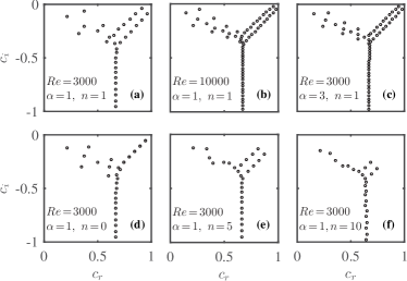
Figure 1: Spectra for parameters shown in each panels. Other parameters:(a) $N=47$; (b) $N=68$; (c) $N=69$; (d) $N=53$; (e) $N=53$; (f) $N=53$;

The sub-figures show the overall converged spectrum. As can be observed from the caption of Fig. 1, an increase in the number of collocation points is needed when there is an increase in $\alpha$, shown in Fig. 1(c), or $Re$, Fig. 1(b), but seldom for an increase in $n$, shown in Fig. 1(e) and (f). However, it should be observed that there is a surfacing of mild distortion in the spectrum for $n=10$ with $\alpha=1$ and $Re=3000$ as shown in Fig. 1(f). This can be explained using Eq. (4). It is well-known that the non-normality is caused by the convective terms that interact with mean shear. These terms are enhanced for large values of $n$ by the first term on the RHS of Eq. (4) giving rise to such distortions. The spectrum in Fig. 1(b) has same parameters as a sub-figure of Fig. 1 of Meseguer & Trefethen [22] and can be compared as a validation. For the case of $\{n=0,\alpha=1\}$ shown in Fig. 1(d), the two wall-mode branches appears to have merged at the accuracy of the figure. As the azimuthal wavenumber is increased the number of modes in the centre branch decrease as shown in Fig. 1(e) and (f).

Table 2 compares the spectrum obtained for the case of $\{\alpha=0,n=0\}$ from the system of Eqs. (23)-(24) with those obtained from the characteristic relations given by Eqs. (39)-(40). These characteristic relations have been approximated by polynomials, as explained in the caption of Table 2, by setting a cut-off value of 90 for the running index $k$ in the summation.

Table 2: Comparison of first seven least decaying eigenvalues, $\omega_{i}$’s for the case of $\{\alpha=0,n=0\}$ with $Re=3000$ and $N=47$ obtained from system of Eq. (23)-(24) versus those obtained from $\omega_{i}=\lambda Re/4$ where the $\lambda$’s are the real solutions of the characteristic Eq. (39)-(40) approximated with the setting $\max\{k\}=90$. The reported figures are of the converged accuracy with respect to $N$ and $\max\{k\}$.

$\omega_{i}$’s from Eq. (23)	$\lambda Re/4$ with $\lambda$’s from Eq. (39)
$-0\cdot 001927728654315596$	$-0\cdot 0019277286543156$
$-0\cdot 01015708744788736$	$-0\cdot 010157087447887$
$-0\cdot 02496233559689843$	$-0\cdot 024962335596$
$-0\cdot 04634676147548659$	$-0\cdot 046346761475$
$-0\cdot 0743107678725448$	$-0\cdot 07431076787$
$-0\cdot 108854450977443$	$-0\cdot 108854450$
$-0\cdot 149977842839345$	$-0\cdot 14997784$
$\omega_{i}$’s from Eq. (24)	$\lambda Re/4$ with $\lambda$’s from Eq. (40)
$-0\cdot 004893990214041297$	$-0\cdot 0048939902140412$
$-0\cdot 01640615210723253$	$-0\cdot 01640615210723$
$-0\cdot 03449981796504557$	$-0\cdot 0344998179650$
$-0\cdot 0591735889379348$	$-0\cdot 05917358893$
$-0\cdot 090427218090958$	$-0\cdot 0904272181$
$-0\cdot 128260635034236$	$-0\cdot 12826063$
$-0\cdot 172673813670569$	$-0\cdot 1726738$

In the table, we have shown only the converged decimal figures that does not change when $N$ is changed from $46$ to $47$, or when $\max\{k\}$ is changed from 89 to 90. As can be noted from this table, the results obtained by computation from Eqs. (23)-(24) have higher converging precision in comparison with those given by the characteristic relations Eqs. (39)-(40). The characteristic relations contains a quadratic term of factorials of $k$ in the denominator, which causes loss of precision for large values of $k$. The set value of $\max\{k\}=90$ is the largest that we could afford in the present 64-bit (double precision) calculations. Especially, the highly decaying modes are prone to the precision loss since $|\lambda|$ are large for these modes.

Finally, in Fig. 2 we compare the result from the present system for large wavenumbers with that from solving the system of Burridge & Drazin [14]. The system of Burridge and Drazin is given by

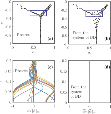
Figure 2: Comparison of spectra and eigenfunctions from the present formulation with that computed from the system of Burridge & Drazin, Eq. (46)-(47). Parameters: $N=200$, $\alpha=10$, $n=7$, $Re=2000$. (a) and (b) are spectra; (c) and (d) are the $\infty-$norm normalized real parts of $\phi$ and $\overline{\phi}$, respectively, close to the centreline of 25 modes selected from the region shown by rectangles in (a) and (b). In (c) $\phi$ has been plotted with respect to $r$ for the purpose of comparison with (d).

$$(\omega-\alpha U)T\overline{\phi}= -\alpha dr^{-1}D\left(rd^{-1}U_{r}\right)\overline{\phi}$$

$$+\mathrm{i}Re^{-1}\left(T^{2}\overline{\phi}-2\alpha nT\overline{\Omega}\right)\quad\text{and}$$ (46)

$$(\omega-\alpha U)\overline{\Omega}= -n(rd)^{-1}U_{r}\overline{\phi}$$

$$+\mathrm{i}Re^{-1}\left(2\alpha nd^{-2}T\overline{\phi}+S\overline{\Omega}\right),$$ (47)

where $D=\frac{\mathop{}\!\mathrm{d}}{\mathop{}\!\mathrm{d}r}$, $\overline{\phi}=-\mathrm{i}rv^{\prime}$ and $\overline{\Omega}=(\alpha rw^{\prime}-nu^{\prime})/d$, and the operators $T$ and $S$ are defined as $T[\cdot]=dr^{-1}D(rd^{-1}D[\cdot])-dr^{-2}[\cdot]$ and $S[\cdot]=(rd)^{-1}D(rdD[\cdot])-dr^{-2}[\cdot]$. The boundary conditions are given in Schmid & Henningson [32]. (However, there is a trivial typographical sign error in the first term of Eq. (3.41) in that reference. The system of Burridge & Drazin as it appear in Ref. [14], has a typographical error in the definition of operator, $T$.)

As can be noted from Fig. 2(a) and (b), the computation from the system, Eq. (46)-(47), suffers from pseudospectra, which is absent in the present formulation. This can be understood as follows. In Fig. 2(a) and (b) the blue rectangle shows a region of the spectrum containing 25 modes that undergoes distortion when computation is performed from the system of Burridge and Drazin. Fig. 2(c) and (d) shows $\phi$’s of the modes that are present within those rectangles. As mentioned earlier, the components of eigenfunctions of the present formulation, $\phi$ for example, undergoes steep variations close to the centreline for large $\alpha$. Such variations have been suppressed in the case of the system of Eq. (46)-(47), as $\overline{\phi}=-\mathrm{i}r^{n}\phi$, which shows that Burridge and Drazin’s unknown $\overline{\phi}$ is a multiplication of the present unknown $\phi$ by a function that is vanishingly small for a range of the domain. When $n$ is large, $\overline{\phi}$ is closer to zero for almost a fifth of the pipe radius as can be seen from Fig. 2(d) for the modes of distorted regions of the spectrum shown in Fig. 2(b). This implies that the details of the factor of $\phi$ in the expression for $\overline{\phi}(=-\mathrm{i}r^{n}\phi)$, where the former, i.e., $\phi$ is the distinguishing feature among different eigenfunctions, would be poorly represented even at double precision. For evidence that the distortion of the spectrum in Fig. 2(b) originiates in round-off errors, one can note that this pattern is similar to Fig. 2(b) of Ref. [7], which shows a spectrum in 16 bit, although for a set of small values of parameters, i.e., $\alpha$, $n$ and $Re$.

Let us assume that we cast Eqs. (46)-(46) in the form of $Re^{-1}\bm{\overline{A}}\bm{\overline{q}}=\omega\bm{\overline{B}}\bm{\overline{q}}$ where $\overline{\overline{q}}=(\overline{\phi},\overline{\Omega})^{\rm T}$, similar to the present formulation as we saw in Eq. (44). Let us compare the condition numbers, $\text{cond}(\bm{L}-\omega I)$ and $\text{cond}(\bm{\overline{L}}-\omega I)$ where $\bm{L}=\bm{B}^{-1}\bm{A}/Re$ and $\bm{\overline{L}}=\bm{\overline{B}}^{-1}\bm{\overline{A}}/Re$. We found that $\text{cond}(\bm{\overline{L}}-\omega I)\sim O(10^{18})$ and $\text{cond}(\bm{L}-\omega I)\sim O(10^{21})$, for $\omega^{\prime}s$ chosen from their respective rectangles shown in Fig. 2(a) and (b). This shows that the present eigensystem is much closer to singularity for these modes than that of Burridge and Drazin. In other words, the contours of resolvent norms in the complex plane will be of smaller value for the same radial distance from these eigenvalues in the present formulation in comparison with the system of Burridge and Drazin.

4 Inviscid Algebraic Instability of Axially constant Modes

In this section we deduce the present flow configuration’s analogue of the findings of Ellingsen and Palm [24] for plane shear flows for the streamwise constant modes. The aim is to find the initial $\phi$ and $\Omega$, i.e. at time $t=0$, that maximizes the energy amplification, and the output pattern at a later time $t$. Ellingsen and Palm solution concerns inviscid solutions with $\alpha=0$ in a non-modal setting and results in a initial value problem. (For such initial value problem in viscous scenario, see Ref. [34] for series solutions, and Ref. [7] for optimal patterns). For axially constant inviscid modes that has a general non-modal time dependence, Eq. (19) and (20) become

$$\frac{\partial}{\partial t}\left[(\ell+2)\mathcal{D}\phi+y\mathcal{D}^{2}\phi\right]= 0$$ (48)

$$\frac{\partial\Omega}{\partial t}= -2\mathrm{i}nU_{y}\phi.$$ (49)

The Eq. (48) implies conservation of kinetic energy in the radial and azimuthal directions. As will be shown later in this section, the sum of energies in these directions is proportional to $(\ell+2)\mathcal{D}\phi+y\mathcal{D}^{2}\phi$ (apart from a factor of $-2n^{-2}y^{\ell+1}$). Eq. (48) governs the rate at which energy is pumped into the radial vorticity by the mean shear. Since the azimuthal velocity is conserved, this implies the rate at which the axial component of the kinetic energy is enhanced, giving rise to streaks.

Eq. (48) can be readily integrated to yield $(\ell+2)\mathcal{D}\phi+y\mathcal{D}^{2}\phi=C(y)$, where the function, $C(y)=[(\ell+2)\mathcal{D}\phi+y\mathcal{D}^{2}\phi]|_{t=0}$ is equivalent to the specification of an initial value of the kinetic energy in the non-streamwise directions. Such specification of $C(y)$ at $t=0$ is equivalent to the specification of $\phi_{0}$, the initial value of $\phi$ itself. (In fact, for a specified $C(y)$, the $\phi_{0}(y)$ that is finite at centreline and satisfying $\phi_{0}(1)=0$ is given by $\phi_{0}(y)=\int_{0}^{1}[\mathcal{U}(y-\overline{y})-1]{\overline{y}}^{-(\ell+2)}\int_{0}^{\overline{y}}C(\tilde{y})\tilde{y}^{\ell+1}\mathop{}\!\mathrm{d}\tilde{y}\mathop{}\!\mathrm{d}\overline{y}$ where $\mathcal{U}(y)$ is the unit step function). Therefore,

$$\phi(t,y)= \phi_{0}(y)$$ (50)

$$\Omega(t,y)= \Omega_{0}(y)-2\mathrm{i}nU_{y}t\phi_{0}(y),$$ (51)

where $\Omega_{0}(y)=\Omega(t=0,y)$. Eq. (51) is obtained from integration of Eq. (49) and describes algebraic growth since the second term is secular, which implies the collapse of linear perturbation theory after certain initial time unless viscosity acts and kills it. In terms of velocities these equations translate into: $v^{\prime}(t,y)=v^{\prime}(0,y)$, $u^{\prime}(t,y)=u^{\prime}(0,y)-2t\sqrt{y}U_{y}v^{\prime}(0,y)$ and $w^{\prime}(t,y)=\mathrm{i}n^{-1}[v^{\prime}(0,y)+2y\mathcal{D}v^{\prime}(0,y)]$.

To find the optimal patterns in this inviscid limit, we follow the method of Ref. [35] for compressible flow with necessary modifications for the present incompressible configurations (see also Ref [36]). As we are working with a 2-tuple variable, the constraint of continuity is already taken into consideration. The energy, $E(t)\equiv 2^{-1}\int_{0}^{1}|\bm{u^{\prime}}|^{2}dy$ can be written with the help of Eq. (8)-(14) as

$$E(t)=\frac{1}{2n^{2}}\int_{0}^{1}\left[y^{\ell+1}|\Omega|^{2}+2n^{2}y^{\ell}|\phi|^{2}+4y^{\ell+2}|\mathcal{D}\phi|^{2}\right.\\ \left.+2(\ell+1)y^{\ell+1}\left(\phi^{*}\mathcal{D}\phi+\phi\mathcal{D}\phi^{*}\right)\right]\mathop{}\!\mathrm{d}y,$$ (52)

which can be written after integration by parts as,

$$E(t)=(2n^{2})^{-1}\int_{0}^{y}y^{\ell+1}\bm{q_{0}^{\text{H}}\mathcal{A}^{\text{H}}\mathcal{MA}q_{0}}\mathop{}\!\mathrm{d}y,$$ (53)

where $\bm{q_{0}}=\{\phi_{0},\Omega_{0}\}^{\textrm{T}}$, the positive definite $2\times 2$ matrix $\bm{\mathcal{M}}=\textrm{diag}\{-4[(\ell+2)\mathcal{D}+y\mathcal{D}^{2}],1\}$. The operator $\bm{\mathcal{A}}$ is the propagator of $\bm{q_{0}}$ and can be obtained by casting Eq. (50) and Eq. (51) in matrix form. The elements of $\bm{\mathcal{A}}$ are $\mathcal{A}_{11}=\mathcal{A}_{22}=1$, $\mathcal{A}_{12}=0$, and $\mathcal{A}_{21}=-2\mathrm{i}nU_{y}t$. Let $g(t)$ be the propagator of the initial energy, i.e.,

$$E(t)=g(t)E(0).$$ (54)

Note that $E(0)=(2n^{2})^{-1}\int_{0}^{y}y^{\ell+1}\bm{q_{0}^{\text{H}}\mathcal{M}q_{0}}\mathop{}\!\mathrm{d}y$. Let us define, $G(t)=\max_{\bm{q_{0}}}g(t)$. This $G(t)$ is found as follows. Taking the functional derivative of Eq. (54), we get

$$\frac{\delta}{\delta\bm{q_{0}}^{\text{H}}}E(t)=\left(\frac{\delta}{\delta\bm{q_{0}}^{\text{H}}}g(t)\right)E(0)+g(t)\frac{\delta}{\delta\bm{q_{0}}^{\text{H}}}E(0).$$ (55)

Setting $\delta g/\delta\bm{q_{0}}^{\text{H}}=0$ for maximization we get,

$$\bm{\mathcal{A}^{\text{H}}\mathcal{MA}q_{0}}=g(t)\bm{\mathcal{M}q_{0}},$$ (56)

which is a differential equation that can also be written as

$$2\left[(nU_{y}t)^{2}-(\ell+2)\mathcal{D}-y\mathcal{D}^{2}\right]\phi_{0}+\mathrm{i}nU_{y}t\Omega_{0}\\ =-2g(t)\left[(\ell+2)\mathcal{D}+y\mathcal{D}^{2}\right]\phi_{0}$$ (57)

$$-2\mathrm{i}nU_{y}t\phi_{0}+\Omega_{0}=g(t)\Omega_{0}$$ (58)

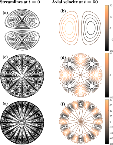
Figure 3: The inviscid initial (left) and the instantaneous velocity patterns at a later time (right) for axially constant modes that are optimized for maximum energy growth: (a) and (b) $n=1$; (c) and (d) $n=4$; and, (e) and (f) $n=10$. The sub-figures on the left column are the 2D streamlines in the cross section of the pipe at time, $t=0$. The sub-figures on the right column are the contours of the axial velocity at time, $t=50$ with levels indicated by colour-bar.

This is an eigenvalue problem with the Lagrange multiplier, $g(t)$, as the eigenvalue for a chosen $t$. Since the operators are Hermitian, $g(t)$’s are all real, and as $\mathcal{M}$ is positive definite by definition, $g(t)$’s are all positive. The boundary conditions are no-penetration at the wall and regularity at the centreline, i.e., $\phi_{0}(1)=0$ and $2[(g(t)-1)(\ell+2)\mathcal{D}+(nU_{y}t)^{2}]_{y=0}\phi_{0}+\mathrm{i}nU_{y}t\Omega_{0}(0)=0$, respectively. As $\Omega_{0}$ appears algebraically in Eq. (58), it does not require boundary conditions. In fact, we can explicitly solve for $\Omega_{0}$ in terms of $\phi_{0}$ and express Eq. (56) as an eigenvalue problem with only $\phi_{0}$ as the unknown. However, this will lead to that the eigenvalue parameter, $g(t)$, appears quadratically and will warrant a companion matrix method to solve the equation numerically, which is equivalent to the problem as it appears currently in Eq. (56). The maximum amplification, $G(t)$ as defined above, is given by $G(t)=\max_{j}g_{j}(t)$ where $g_{j}(t)$’s for a chosen $t$ are the set of eigenvalues of Eq. (56). However, the variation $G(t)\sim t^{2}$ can be anticipated from Eq. (51). In addition, such a variation of $G(t)$ with respect to $t$ has been observed in wall-bounded plane shear flows [37]. Here, we focus is on the optimal $\bm{q_{0}}$ and the corresponding $\bm{q}(t)$ as obtained from Eq. (56). To solve the system given by Eq. (56), we adopt the the spectral method described in previous section.

Figs. 3(a), (c) and (e) show the streamlines of initial velocity pattern in the cross sectional plane for $n=1,4\ \text{and}\ 10$, respectively, that are prone to the maximum energy amplification. These patterns represent counter rotating vortices. The explanation for the appearance of these patterns is similar to the case of plane shear flows, such as boundary layer, Couette and plane Poiseuille flows. Since counter rotating vortices contain movement of fluid particles in the radial direction, they can transfer energy from mean shear into axial velocity. This phenomenon is widely known as lift-up effect [32] in these plane shear flows. In the context of this pipe flow, the term, up refers to the radial direction.

Such patterns have been observed in this flow configuration through DNS of full nonlinear viscous equations when the mean flow was perturbed initially with axially constant modes [25]. Fig. 3(a) matches with the optimal pattern from the viscous flow computation at $Re=3000$ shown in Ref. [22]. Since this inviscid analysis captures those features, one can conclude that the inviscid lift-up effect is dominant at initial times before viscosity break this vortices into small scales. Figs. 3(b), (d) and (f) show the contours of axial component of perturbation velocity at a later time chosen as $t=50$ in the non-dimensional scale, where the initial state $\bm{q_{0}}$ has been normalized such that $E(0)=1$. These patterns describe near-wall streaks when superimposed with the mean flow. These streaks are known to be the characteristic feature of bypass transition. (For a matching of these optimal perturbations with experimental data in the case of boundary layers, see [38]). As the value of $n$ is increased, these streaks are pushed closer to the wall, a result tied to the following two facts: (1) The streamwise velocity’s growth is proportional to the radial velocity as can be seen from the relation, $u^{\prime}(t,y)=u^{\prime}(0,y)-2t\sqrt{y}U_{y}v^{\prime}(0,y)$; and, (2) the radial velocity culminates at the periphery of the cross-section when $n$ is increased as can be to noted from $v^{\prime}=r^{l}\phi_{0}$.

It should be noted that the $G(t)$ at a chosen time would increase with an increase in $n$ as evident from Eq. (51). This also shows up on the range of the colour bars in Fig. 3 as we move down from panels (b) to (f). However, as can be seen from the optimal patterns (in the inviscid limit), the size of these vortices reduces when $n$ is increased, making them more prone to the action of viscosity to break them further and eventually being killed. This phenomenon can be observed from Fig.4(a) of Ref. [7] and Fig.4 of Ref. [39].

5 Conclusion

The present formulation, which uses the ansatz of Priymak & Miyazaki [19] results in accurate spectra even for reasonably large values of the parameters, namely, the wavenumbers and Reynolds number. The obtained accuracy is on par with that of Meseguer & Trefethen [21]. However, as the boundary conditions of the wall are directly imposed on the unknowns used, which is in contrast to that of Meseguer & Trefethen [21], where they are imposed on the basis functions, the present formulation enables the derived system to be applied on a range of flow configurations with various boundary conditions.

The multiplicity of the poles of regular singularity yielded the necessary number of regularity conditions in order to complement the boundary conditions at wall, providing 6 conditions to solve the 6th order system for the cases other than that of $\{\alpha=0,n=0\}$.

In the case of $\{\alpha=0,n=0\}$, the working variables had to be changed from a representative of normal vorticity and normal velocity to that of streamwise and azimuthal velocities. The obtained self-adjoint system’s analytical characteristic relation predicted eigenvalues which were used to validate the numerical results for this case. The orthogonality showed that the superposition of these modes are always decaying.

As a demonstration of the performance of this formulation, the results were contrasted against those from the system of Burridge and Drazin [14]. The performance of the current formulation is found to be highlighted at large values of the parameters, and found to postpone the appearance of pseudo-spectra to the regimes of further higher values of these parameters. This was tracked to the fact that the numerical representation of distinctive features of different eigenfunctions are enhanced in the present formulation, and that it undergoes precision loss in the case of Burridge and Drazin due to round-off errors.

Finally, the inviscid algebraic (nonmodal) growth of the perturbation for streamwise constant modes were studied. The result was the pipe flow’s counterpart of Ellingsen and Palm solutions for plane shear flows. The present working variables for the unknowns and the independent variable, $y$, resulted in the solutions which were almost identical in structure to that of plane shear-flows, hence retaining the well known characteristics such as having the counter rotating vortices and streaks as optimal patterns. These streaks were found to be closer to the wall when the azimuthal wavenumber is larger. For the appearance of such streaks, it is not necessary that the infinitesimal perturbations acquired through receptivity should have the Fourier components with $n$ very large. The nonlinearity can play the role even at very early stages to give birth to such modes through convolution of modes with lower $n$, and subsequently amplified by the linear mechanism of lift-up.

Appendix A Operators and functions

To facilitate locating the functions and operators below, their names have been given in boldface. $\bm{L_{1}}=(f_{1}+f_{2}D+rd^{-1}D^{2})$, $\bm{L_{2}}=(f_{3}+d^{-1}D)$, $\bm{L_{3}}=(f_{4}+f_{5}D+\alpha^{2}rUd^{-1}D^{2})$, $\bm{L_{4}}=d^{-1}(f_{6}+UD)$, $\bm{L_{5}}=(f_{7}+f_{8}D+f_{9}D^{2}+f_{10}D^{3}+rd^{-1}D^{4})$, $\bm{L_{6}}=(f_{11}+f_{12}D+f_{13}D^{2}+d^{-1}D^{3})$, $\bm{L_{7}}=f_{14}+f_{15}D+(rd)^{-1}D^{2}$, $\bm{L_{8}}=f_{16}+d^{-1}D$, $\bm{L_{9}}=f_{17}+U_{r}(rd)^{-1}D$, $\bm{L_{10}}=d^{-1}(U_{r}+UD)$, $\bm{L_{11}}=f_{18}+f_{19}D+f_{20}D^{2}+f_{21}D^{3}+(rd)^{-1}D^{4}$, $\bm{L_{12}}=f_{22}+f_{23}D+f_{24}D^{2}+d^{-1}D^{3}$, $\bm{L_{13}}=f_{25}-f_{26}D-d^{-1}D^{2}$, $\bm{L_{14}}=f_{27}+f_{28}D+D^{2}$, $\bm{L_{15}}=f_{29}+f_{30}D+f_{31}D^{2}+f_{32}D^{3}+r^{2}D^{4}$, $\bm{L_{16}}=f_{33}+f_{34}D+r^{2}d^{-1}D^{2}$

$\bm{f_{1}}=[(\ell+1)d_{2}-d^{2}]/(d^{2}r)$, $\bm{f_{2}}=[d_{2}+(\ell+2)d]/d^{2}$, $\bm{f_{3}}=d_{2}/(d^{2}r)$, $\bm{f_{4}}=[U_{r}(\alpha^{2}r^{2}-n^{2}\ell)-rdU_{rr}]/(dr^{2})$, $\bm{f_{5}}=-n^{2}U_{r}/(rd)$, $\bm{f_{6}}=(Ud_{2}+rdU_{r})/(rd)$, $\bm{f_{7}}=[(\ell+1)(d_{4}+dd_{3}-(d+1)d_{2}d^{2})+(d+1-\ell^{2})d^{4}]/(d^{4}r^{3})$, $\bm{f_{8}}=[d_{4}+(3\ell+7)dd_{3}+(2\ell+3-d)d^{2}d_{2}-3(\ell+1)d^{4}-(\ell+2)d^{3}]/(d^{4}r^{2})$, $\bm{f_{9}}=[3d_{3}+(3\ell+11)dd_{2}+(\ell+2-2d)d^{2}]/(rd^{3})$, $\bm{f_{10}}=[3d_{2}+(\ell+5)d]/d^{2}$, $\bm{f_{11}}=[d_{4}+dd_{3}-(d+1)d^{2}d_{2}+2d^{4}]/(d^{4}r^{3})$, $\bm{f_{12}}=[3d_{3}+2dd_{2}-(d+1)d^{2}]/(d^{3}r^{2})$, $\bm{f_{13}}=[3d_{2}+d]/(d^{2}r)$,

$\bm{f_{14}}=[(\ell+1)(d+d_{5})-d^{2}]/(d^{2}r^{3})$, $\bm{f_{15}}=[d_{5}+(\ell+3)d]/(d^{2}r^{2})$, $\bm{f_{16}}=(d_{5}+3d)/(rd^{2})$, $\bm{f_{17}}=(\ell+1)U_{r}/(r^{2}d)$, $\bm{f_{18}}=(\ell+1)(r^{5}d^{4})^{-1}[d_{7}+2dd_{6}-(d+1)d^{2}d_{5}+(1-d)d^{3}]+r^{-5}(d-\ell^{2}+2\ell-1)$, $\bm{f_{19}}=[d_{7}+(3\ell+8)dd_{6}+(4\ell+7-d)d^{2}d_{5}-(\ell+1)d^{3}-(3\ell+2)d^{4}]/(rd)^{4}$, $\bm{f_{20}}=[3d_{6}+(3\ell+13)dd_{5}+(2\ell+5)d^{2}-2d^{3}]/(rd)^{3}$, $\bm{f_{21}}=[3d_{5}+(\ell+6)d]/(rd)^{2}$, $\bm{f_{22}}=[d_{7}+8dd_{6}+(13-d)d^{2}d_{5}+3(1-d)d^{3}]/(d^{4}r^{3})$, $\bm{f_{23}}=(3d_{6}+15dd_{5}+13d^{2}-d^{3})/(d^{3}r^{2})$, $\bm{f_{24}}=(3d_{5}+8d)/(d^{2}r)$,

$\bm{f_{25}}=[d^{2}-(\ell+1)d_{2}]/(rd)^{2}$, $\bm{f_{26}}=[d_{2}+(\ell+2)d]/(d^{2}r)$, $\bm{f_{27}}=[(\ell^{2}-d-1)d^{2}+2n^{2}d_{2}]/(rd)^{2}$, $\bm{f_{28}}=[(2\ell+1)d+2n^{2}]/(rd)$, $\bm{f_{29}}=[(\ell+1)(d_{4}-d^{3}d_{2}-d_{1}d_{3}+dd_{1}d_{2})+(d-\ell^{2})d^{4}+(2\ell n^{2}-d_{1})d^{3}]/(d^{3}r^{2})$, $\bm{f_{30}}=[d_{4}+2(2\ell+3)dd_{3}-d_{2}d_{3}-2(2\ell+1)d^{4}+(\ell+2)d^{2}d_{1}-(2\ell+3)dd_{1}d_{2}]/(d^{3}r)$, $\bm{f_{31}}=[3d_{3}+(5\ell+9)dd_{2}-2d_{2}^{2}-(\ell+2)dd_{1}-2d^{3}]/d^{2}$, $\bm{f_{32}}=2r[d_{2}+(\ell+2)d]/d$, $\bm{f_{33}}=(d_{3}+dd_{2}-d^{3})/d^{3}$, $\bm{f_{34}}=r[2d_{2}+d]/d^{2}$

$\bm{d_{1}}=n^{2}-\alpha^{2}r^{2}$, $\bm{d_{2}}=(\ell+1)d-2\alpha^{2}r^{2}$, $\bm{d_{3}}=(\ell d-4\alpha^{2}r^{2})d_{2}+2(\ell-1)\alpha^{2}r^{2}d$, $\bm{d_{4}}=(\ell-1)dd_{3}-6\alpha^{2}r^{2}d_{3}+2\alpha^{2}r^{2}d[(\ell-4)d_{2}+(\ell-1)(\ell+2)d-2(\ell-1)\alpha^{2}r^{2}]$, $\bm{d_{5}}=\ell d-2\alpha^{2}r^{2}$, $\bm{d_{6}}=(\ell-1)dd_{5}-4\alpha^{2}r^{2}d_{5}+2(\ell-2)\alpha^{2}r^{2}d$, $\bm{d_{7}}=(\ell-2)dd_{6}-6\alpha^{2}r^{2}d_{6}+2\alpha^{2}r^{2}d[(\ell-5)d_{5}+(\ell-2)(\ell+1)d-2(\ell-2)\alpha^{2}r^{2}]$

$\bm{g_{1}}=n^{6}+2(\ell+1)n^{4}+n^{2}[3n^{2}+4(\ell+1)]\alpha^{2}y+[3n^{2}+2(\ell+1)]\alpha^{4}y^{2}+\alpha^{6}y^{3}$, $\bm{g_{2}}=4(\ell+2)n^{6}+4n^{4}(3\ell+5)\alpha^{2}y+4n^{2}(3\ell+4)\alpha^{4}y^{2}+4(\ell+1)\alpha^{6}y^{3}$, $\bm{g_{3}}=n^{2}(\ell^{4}+8\ell^{3}+26\ell^{2}+32\ell+13)+(3\ell^{4}+20\ell^{3}+50\ell^{2}+36\ell+3)\alpha^{2}y+(3\ell^{2}+10\ell+7)\alpha^{4}y^{2}+\alpha^{6}y^{3}$, $\bm{g_{4}}=n^{4}(\ell^{3}+6\ell^{2}+11\ell+6)+n^{2}(3\ell^{3}+15\ell^{2}+21\ell+5)\alpha^{2}y+(3\ell^{3}+12\ell^{2}+13\ell+4)\alpha^{4}y^{2}+(\ell+1)\alpha^{6}y^{3}$, $\bm{g_{5}}=8[n^{6}(2\ell^{2}+10\ell+12)+n^{4}(5\ell^{2}+22\ell+21)\alpha^{2}y+n^{2}(3\ell^{2}+12\ell+9)\alpha^{4}y^{2}-n^{2}\alpha^{6}y^{3}-\alpha^{8}y^{4}]$, $\bm{g_{6}}=n^{2}+2(\ell+1)+\alpha^{2}y$, $\bm{g_{7}}=n^{2}(\ell^{2}+4\ell+7)+2(\ell^{2}+3\ell+2)\alpha^{2}y+\alpha^{4}y^{2}$, $\bm{g_{8}}=n^{2}[3n^{2}+4(\ell+1)]$, $\bm{g_{9}}=n^{4}[2(5\ell+9)-n^{2}]$, $\bm{g_{10}}=4n^{6}(\ell+3)$, $\bm{g_{11}}=n^{4}[n^{2}+2\ell+18]$, $\bm{g_{12}}=3\ell^{4}+20\ell^{3}+50\ell^{2}+36\ell+3$, $\bm{g_{13}}=n^{2}(\ell^{4}-16\ell^{3}-94\ell^{2}-136\ell-27)$, $\bm{g_{14}}=8n^{4}(\ell^{3}+\ell^{2}-11\ell-15)$, $\bm{g_{15}}=16n^{6}(\ell^{2}+7\ell+12)$

Appendix B MATLAB Code

References

- [1] T. Itano, S. Toh, The dynamics of bursting process in wall turbulence, Journal of the Physical Society of Japan 70 (3) (2001) 703–716 (2001).
- [2] T. M. Schneider, B. Eckhardt, J. A. Yorke, Turbulence transition and the edge of chaos in pipe flow, Physical review letters 99 (3) (2007) 034502 (2007).
- [3] N. B. Budanur, B. Hof, Complexity of the laminar-turbulent boundary in pipe flow, Physical Review Fluids 3 (5) (2018) 054401 (2018).
- [4] L. Böberg, U. Brosa, Onset of turbulence in a pipe, Zeitschrift für Naturforschung A 43 (8-9) (1988) 697–726 (1988).
- [5] K. M. Butler, B. F. Farrell, Three-dimensional optimal perturbations in viscous shear flow, Physics of Fluids A: Fluid Dynamics 4 (8) (1992) 1637–1650 (1992).
- [6] L. N. Trefethen, A. E. Trefethen, S. C. Reddy, T. A. Driscoll, Hydrodynamic stability without eigenvalues, Science 261 (5121) (1993) 578–584 (1993).
- [7] P. J. Schmid, D. S. Henningson, Optimal energy density growth in hagen–poiseuille flow, Journal of Fluid Mechanics 277 (1994) 197–225 (1994).
- [8] P. J. Schmid, Nonmodal stability theory, Annu. Rev. Fluid Mech. 39 (2007) 129–162 (2007).
- [9] M. Gavarini, A. Bottaro, F. Nieuwstadt, The initial stage of transition in pipe flow: role of optimal base-flow distortions, Journal of Fluid Mechanics 517 (2004) 131–165 (2004).
- [10] K. C. Sahu, R. Govindarajan, Stability of flow through a slowly diverging pipe, Journal of Fluid Mechanics 531 (2005) 325–334 (2005).
- [11] S. Loh, H. Blackburn, Stability of steady flow through an axially corrugated pipe, Physics of Fluids 23 (11) (2011) 111703 (2011).
- [12] V. Pruša, On the influence of boundary condition on stability of hagen–poiseuille flow, Computers & Mathematics with Applications 57 (5) (2009) 763–771 (2009).
- [13] M. Lessen, S. G. Sadler, T.-Y. Liu, Stability of pipe poiseuille flow, The Physics of Fluids 11 (7) (1968) 1404–1409 (1968).
- [14] D. Burridge, P. Drazin, Comments on “stability of pipe poiseuille flow”, The Physics of Fluids 12 (1) (1969) 264–265 (1969).
- [15] H. Salwen, C. E. Grosch, The stability of poiseuille flow in a pipe of circular cross-section, Journal of Fluid Mechanics 54 (1) (1972) 93–112 (1972).
- [16] H. Salwen, F. W. Cotton, C. E. Grosch, Linear stability of poiseuille flow in a circular pipe, Journal of Fluid Mechanics 98 (2) (1980) 273–284 (1980).
- [17] P. O’sullivan, K. Breuer, Transient growth in circular pipe flow. I. linear disturbances, Physics of fluids 6 (11) (1994) 3643–3651 (1994).
- [18] C. Thomas, A. Bassom, P. Blennerhassett, The linear stability of oscillating pipe flow, Physics of Fluids 24 (1) (2012) 014106 (2012).
- [19] V. Priymak, T. Miyazaki, Accurate navier–stokes investigation of transitional and turbulent flows in a circular pipe, Journal of Computational Physics 142 (2) (1998) 370–411 (1998).
- [20] M. R. Khorrami, M. R. Malik, R. L. Ash, Application of spectral collocation techniques to the stability of swirling flows, Journal of Computational Physics 81 (1) (1989) 206–229 (1989).
- [21] A. Meseguer, L. Trefethen, A spectral petrov-galerkin formulation for pipe flow I: linear stability and transient growth, Tech. rep., Oxford University Computing Laboratory (2000).
- [22] A. Meseguer, L. N. Trefethen, Linearized pipe flow to reynolds number , Journal of Computational Physics 186 (1) (2003) 178–197 (2003).
- [23] M. Malik, M. Skote, R. Bouffanais, Growth mechanisms of perturbations in boundary layers over a compliant wall, Physical Review Fluids 3 (1) (2018) 013903 (2018).
- [24] T. Ellingsen, E. Palm, Stability of linear flow, The Physics of Fluids 18 (4) (1975) 487–488 (1975).
- [25] O. Y. Zikanov, On the instability of pipe poiseuille flow, Physics of Fluids 8 (11) (1996) 2923–2932 (1996).
- [26] W. E. Boyce, R. C. DiPrima, Elementary differential equations and boundary value problems., John Wiley & Sons, 2009 (2009).
- [27] C. Foias, O. Manley, R. Rosa, R. Temam, Navier-Stokes equations and turbulence, Vol. 83, Cambridge University Press, 2001 (2001).
- [28] B. Rummler, The eigenfunctions of the stokes operator in special domains. I, ZAMM-Journal of Applied Mathematics and Mechanics/Zeitschrift für Angewandte Mathematik und Mechanik 77 (8) (1997) 619–627 (1997).
- [29] B. Rummler, The eigenfunctions of the stokes operator in special domains. II, ZAMM-Journal of Applied Mathematics and Mechanics/Zeitschrift für Angewandte Mathematik und Mechanik 77 (9) (1997) 669–675 (1997).
- [30] P. F. Batcho, G. E. Karniadakis, Generalized stokes eigenfunctions: a new trial basis for the solution of incompressible navier-stokes equations, Journal of Computational Physics 115 (1) (1994) 121–146 (1994).
- [31] L. N. Trefethen, Spectral methods in MATLAB, Vol. 10, Siam, 2000 (2000).
- [32] P. J. Schmid, D. S. Henningson, Stability and transition in shear flows, Vol. 142, Springer Verlag, 2001 (2001).
- [33] G. H. Golub, C. F. Van Loan, Matrix computations, 3rd Edition, JHU press, 1996 (1996).
- [34] L. Bergström, Initial algebraic growth of small angular dependent disturbances in pipe poiseuille flow, Studies in Applied Mathematics 87 (1) (1992) 61–79 (1992).
- [35] A. Hanifi, D. S. Henningson, The compressible inviscid algebraic instability for streamwise independent disturbances, Physics of Fluids 10 (8) (1998) 1784–1786 (1998).
- [36] M. Malik, J. Dey, M. Alam, Linear stability, transient energy growth, and the role of viscosity stratification in compressible plane couette flow, Physical Review E 77 (3) (2008) 036322 (2008).
- [37] L. H. Gustavsson, Energy growth of three-dimensional disturbances in plane poiseuille flow, Journal of Fluid Mechanics 224 (1991) 241–260 (1991).
- [38] P. Luchini, Reynolds-number-independent instability of the boundary layer over a flat surface: optimal perturbations, Journal of Fluid Mechanics 404 (2000) 289–309 (2000).
- [39] L. Bergström, Optimal growth of small disturbances in pipe poiseuille flow, Physics of Fluids A: Fluid Dynamics 5 (11) (1993) 2710–2720 (1993).