Analytic traveling-wave solutions of the Kardar-Parisi-Zhang interface growing equation with different kind of noise terms

Abstract

The one-dimensional Kardar-Parisi-Zhang dynamic interface growth equation with the traveling-wave Ansatz is analyzed. As a new feature additional analytic terms are added. From the mathematical point of view, these can be considered as various noise distribution functions. Six different cases were investigated among others Gaussian, Lorentzian, white or even pink noise. Analytic solutions are evaluated and analyzed for all cases. All results are expressible with various special functions Mathieu, Bessel, Airy or Whittaker functions showing a very rich mathematical structure with some common general characteristics. This study is the continuation of our former work, where the same physical phenomena was investigated with the self-similar Ansatz. The differences and similarities among the various solutions are enlightened.

Keywords traveling-wave solution  $\cdot$ KPZ equation  $\cdot$ Gaussian noise  $\cdot$ Lorentzian noise  $\cdot$ Special functions  $\cdot$ Heun functions

1 Introduction

Solidification fronts or crystal growth is a scientific topic which attracts much interest from a long time. Basic physics of growing crystallines can be found in large number of textbooks (see e.g., [1]). One of the simplest nonlinear generalization of the ubiquitous diffusion equation is the so called Kardar-Parisi-Zhang (KPZ) model obtained from Langevin equation

$$\frac{\partial u}{\partial t}=\nu{\bf{\nabla}}^{2}u+\frac{\lambda}{2}({\bf{\nabla}}u)^{2}+\eta({\bf{x}},t),$$ (1)

where $u$ stands for the profile of the local growth [2]. The first term on the right hand side describes relaxation of the interface by a surface tension preferring a smooth surface. The next term is the lowest-order nonlinear term that can appear in the surface growth equation justified with the Eden model. The origin of this term lies in non-equilibrium. The third term is a Langevin noise which mimics the stochastic nature of any growth process and usually has a Gaussian distribution. In the last two decades numerous studies came to light about the KPZ equation. Without completeness we mention some of them. The basic physical background of surface growth can be found in the book of Barabási and Stanley [3]. Later, Hwa and Frey [4, 5] investigated the KPZ model with the help of the renormalization group-theory and the self-coupling method which is a precise and sophisticated method using Green’s functions. Various dynamical scaling forms of $C(x,t)=x^{-2\varphi}C(bx,b^{z}t)$ were considered for the correlation function (where $\varphi,b$ and $z$ are real constants). The field theoretical approach by Lässig was to derive and investigate the KPZ equation [6]. Kriecherbauer and Krug wrote a review paper [7], where the KPZ equation was derived from hydrodynamical equations using a general current density relation.

Several models exist and all lead to similar equations as the KPZ model, one of them is the interface growth of bacterial colonies [8]. Additional general interface growing models were developed based on the so-called Kuramoto-Sivashinsky (KS) equation which shows similarity to the KPZ model with an extra $\nabla^{4}u$ term [9], [10].

Kersner and Vicsek investigated the traveling wave dynamics of the singular interface equation [11] which is closely related to the KPZ equation. One may find certain kind of analytic solutions to the problem [12] as already mentioned in [CaDo11].

Ódor and co-worker intensively examined the two dimensional KPZ equation with dynamical simulations to investigate the aging properties of polymers or glasses [13].

Beyond these continuous models based on partial differential equations (PDEs), there are large number of purely numerical methods available to study diverse surface growth effects. As a view we mention the kinetic Monte Carlo [14] model, Lattice-Boltzmann simulations [15], and the etching model [16].

In this paper we investigate the solutions to the KPZ equation with the traveling wave Ansatz in one-dimension applying various forms of the noise term. The effects of the parameters involved in the problem are examined.

2 Theory

In general, non-linear PDEs has no general mathematical theory which could help us to understand general features or to derive physically relevant solutions. Basically, there are two different trial functions (or Ansatz) which have well-founded physical interpretation. The first one is the traveling wave solution, which mimics the wave property of the investigated phenomena described by the non-linear PDE of the form

$$u(x,t)=f(x\pm ct)=f(\omega),$$ (2)

where $c$ means the velocity of the corresponding wave. Gliding and Kersner used the traveling wave Ansatz to investigate study numerous reaction-diffusion equation systems [17]. To describe pattern formation phenomena [18] the traveling waves Ansatz is a useful tool as well. Saarloos investigated the front propagation into unstable states [19], where traveling waves play a key role.

This simple trial function can be generalized in numerous ways, e.g., to $e^{-\alpha t}f(x\pm ct):=e^{-\alpha t}f(\omega)$ which describes exponential decay or to $g(t)\cdot f(x\pm c\cdot t):=g(t)f(\omega)$ which can even be a power law function of the time as well. We note, that the application of these Ansatz to the KPZ equation leads to the triviality of $e^{-\alpha t}=g(t)\equiv 1$. In 2006, He and Wu developed the so-called exp-function method [20] which relying on an Ansatz (a rational combination of exponential functions), involving many unknown parameters to be specified at the stage of solving the problem. The method soon drew the attention of many researchers, who described it as “straightforward”, “reliable”, and “effective”. Later, Aslan and Marinakis [21] summarized various applications of the Ansatz.

There is another existing remarkable Ansatz interpolating the traveling-wave and the self-similar Ansatz by Benhamidouche [22].

The second one is the self-similar Ansatz [23] of the form $u(x,t)=t^{-\alpha}f\left(\frac{x}{t^{\beta}}\right):=t^{-\alpha}f(\omega).$ The associated mathematical and physical properties were exhaustively discussed in our former publications [24], [25] or in a book chapter [26] in the field of hydrodynamics. All these kind of methods belong to the so-called reduction mechanism, where applying a suitable variable transformation the original PDEs or systems of PDEs are reduced to an ordinary differential equation (ODE) or systems of ODEs.

3 Results without the noise term

Applying the traveling wave Ansatz to the KPZ PDE with $\eta(x,t)=0$, equation (1) leads to the ODE of

$$-\nu f^{\prime\prime}(\omega)+f^{\prime}(\omega)\left[c-\frac{\lambda}{2}f^{\prime}(\omega)\right]=0,$$ (3)

From now on we use the Maple 12 mathematical program package to obtain analytic solutions in closed forms. For equation (3), it can be given as

$$f(\omega)=\frac{2}{\lambda}\ln\left(\frac{\lambda\left[c_{1}\nu e^{\frac{c\eta}{\nu}}+c_{2}c\right]}{2\nu c}\right)\nu,$$ (4)

where $c_{1}$ and $c_{2}$ are the constants of integration and $c$ is the speed of the wave.

We fix this notation from now on throughout the paper. Note, that this is an equation of a linear function $f(\omega)=a\omega+b$ (just given in a complicated form) with any kind of parameter set, except $c_{1}=0$ which gives a constant solution. This physically means that there is a continuous surface growing till infinity which is quite unphysical. Therefore, some additional noise is needed to have surface growing phenomena. We remark the general properties of all the forthcoming solutions. Due to the Hopf-Cole transformation [27, 28] $(h=A\ln(y))$ convertes the non-linear KPZ equation to the regular heat conduction (or diffusion) equation with an additional stochastic source term eliminating the non-linear gradient-squared term. All the solutions contain a logarithmic function with a complicated argument. In this sense, the solutions have the same structure, the only basic difference is the kind of special function in the argument. If these argument functions take periodically positive and negative real values then the logarithmic function creates distinct intervals (small islands which describe the surface growing mechanisms, and define the final solution). This statement is generally true for our former study as well [29].

Remark that the solution to (1) obtained from the self-similar Ansatz reads

$$f(\omega)=\frac{2\nu}{\lambda}ln\left(\frac{\lambda c_{1}\sqrt{\pi\nu}\>\>erf[\omega/(2\sqrt{\nu})]+c_{2}}{2\nu}\right),$$ (5)

where $erf[\ ]$ means the error function [30]. Figure 1 compares these two solutions. We note the asymptotic convergence of the self-similar solution and the divergence of the traveling-wave solution. We have the same conclusion as in our former study [29] (where the self-similar Ansatz was applied) , that without any noise term the KPZ equation cannot be applied to describe surface growth phenomena. The different kind of noise terms define different kind of extra islands (parts of the solution having compact supports) and these islands show a growth dynamics.

To have a better understanding between the two solutions, Fig. 2 shows the projection of both complete solutions $u(x,y=0,t).$ The major differences are still present.

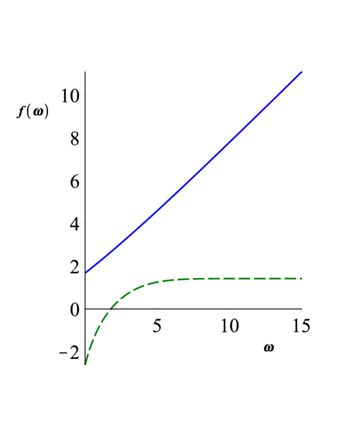
Figure 1: The two shape functions of the KPZ equation without any kind of noise term. The solid line represents the solution for traveling-wave and the dashed line is for the self-similar Ansatz. The applied parameter set is $c_{1}=c_{2}=c=1,\ \nu=4,\ \lambda=3$

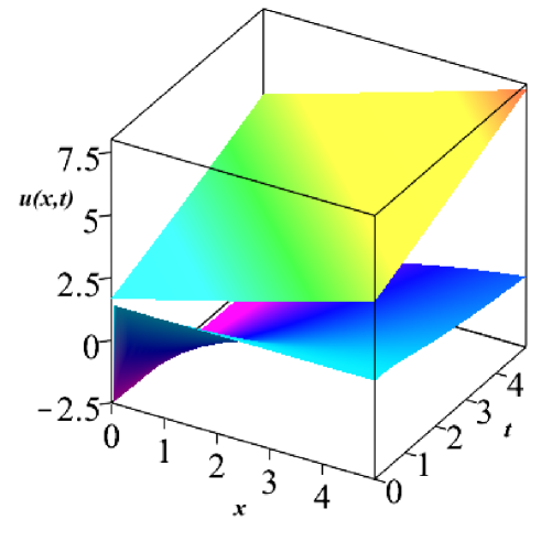
Figure 2: The two solutions of the KPZ equation without any noise term. The upper lying function represents the traveling-wave solution. The applied parameter set is the same as used above.

4 Results with various noise terms

As we mentioned in our former study [29] only the additional noise term makes the KPZ solutions interesting. We search the solutions with the traveling-wave Ansatz, therefore is it necessary that the noise term $\eta$ should be an analytic function of $\omega=x+ct$ like $\eta(\omega)=a(x+ct)^{2}$. We will see that for some kind of noise terms it is not possible to find a closed analytic solution when all the physical parameters are free $(\nu,\lambda,c,a)$, however, if some parameters are fixed it becomes possible to find analytic expressions. It is also clear, that it is impossible to perform a mathematically rigorous complete function analysis according to all four physical and two integral parameters $c_{1},c_{2}$. We performed numerous parameter studies and gave the most relevant parameter dependencies of the solutions.

4.1 Brown noise $n=-2$

As first, case let us consider the brown noise $\eta(x,t)=\frac{a}{\omega^{2}}$. It leads to the following ODE

$$-\nu f^{\prime\prime}(\omega)+f^{\prime}(\omega)\left[c-\frac{\lambda}{2}f^{\prime}(\omega)\right]-\frac{a}{\omega^{2}}=0.$$ (6)

The solution can be given in the form

$$f(\omega)=\frac{1}{\lambda}\left(c\eta+\nu\ln\left\{\frac{\lambda^{2}\left[-c_{1}I_{d}\left(\frac{c\omega}{2\nu}\right)+c_{2}K_{d}\left(\frac{c\omega}{2\nu}\right)\right]^{2}}{c^{2}\omega\left[K_{d}\left(\frac{c\omega}{2\nu}\right)I_{d+1}\left(\frac{c\omega}{2\nu}\right)+I_{d}\left(\frac{c\omega}{2\nu}\right)K_{d+1}\left(\frac{c\omega}{2\nu}\right)\right]^{2}}\right\}\right)$$ (7)

where $I_{d}(\omega)$ and $K_{d}(\omega)$ are the modified Bessel functions of the first and second kind [30] with the subscript of $d=\frac{\sqrt{\nu^{2}-2a\lambda}}{2\nu}+1$. To obtain real solutions for the KPZ equation (which provides the height of the surface) the order of the Bessel function (notated as the subscript) has to be non-negative and provides the following constrain $\nu^{2}\geq 2a\lambda$. This gives us a reasonable relation among the three terms of the right hand side of equation (1). When the magnitude of the noise term $a$ becomes large enough no surface growth take place. Figure 3 presents solutions with different combinations of the integration constants $c_{1},c_{2}$. Having in mind, that the $K_{d}()$ Bessel function of the second kind is regular at infinity, one gets that it has a strong decay at large argument $\omega$. The $c_{1}=0,c_{2}=0$ type solutions have physical relevance. Figure 4 shows the complete solution of the KPZ equation. It can be seen that a sharp and localized peak exists for a short time. Therefore, no typical surface growth phenomena is described with this kind of noise and initial conditions.

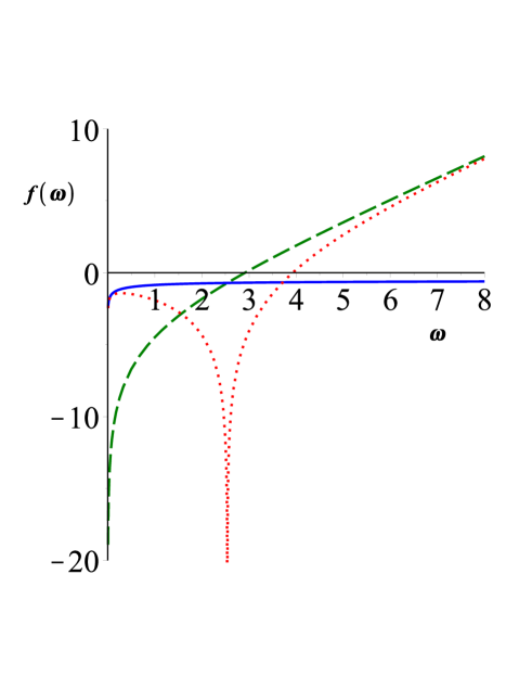
Figure 3: Three different shape functions for the brown noise $n=-2$. The applied physical parameter set is $\lambda=5,\nu=3,a=2$ and $c=2$. The dashed line is for $c_{1}=1,c_{2}=0$, the dotted line is for $c_{1}=c_{2}=1$ and the solid line is for $c_{1}=0,c_{2}=1$, respectively.

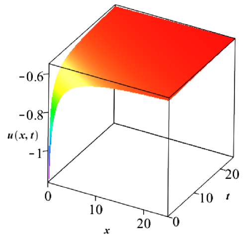
Figure 4: The solution $u(x,t)$ to the KPZ equation for the brown noise $n=-2$ with the parameter set of $c_{1}=c_{2}=c=1,\ \nu=4,\ \lambda=3.$

4.2 Pink noise $n=-1$

The noise term $\eta=\frac{a}{\omega}$ corresponds to the ODE

$$-\nu f^{\prime\prime}(\omega)+f^{\prime}(\omega)\left[c-\frac{\lambda}{2}f^{\prime}(\omega)\right]-\frac{a}{\omega}=0,$$ (8)

whose general solution is

$$f(\omega)=\frac{1}{\lambda}+\ln\left\{\frac{-c\lambda[c_{1}M(\epsilon_{b})-c_{2}U(\epsilon_{b})]}{M(\epsilon_{d})(2\nu cU(\epsilon_{b})+a\lambda U(\epsilon_{b}))+2M(\epsilon_{b})\nu cU(\epsilon_{d})}\right\},$$ (9)

where $M(\epsilon_{b})$ and $U(\epsilon_{d})$ are the Kummer M and Kummer U functions (for more see [30]) with the parameters of $\epsilon_{b}=(\frac{2c\nu-a\lambda}{2c\nu},2,\frac{c\omega}{\nu})$ and $\epsilon_{d}=(\frac{-a\lambda}{2c\nu},2,\frac{c\omega}{\nu})$. Figure 5 shows three different shape functions corresponding to the pink noise. The evaluation of direct parameter dependencies of the solutions are not trivial. In some reasonable parameter range we found the following trends: for fixed $a,c,\nu$ and larger $\lambda$ values, the solution shows more independent well-defined "bumps" or islands and higher steepness of the line which connects the maxima of the existing peaks of the islands. At fixed parameter values $a,c,\lambda$, different values of $\nu$ just shift the position of the existing peaks. The role of $a$ and $c$ is not defined. Figure 6 presents a total solution $u(x,t)$ to the KPZ equation, the freely traveling three islands are clearly seen.

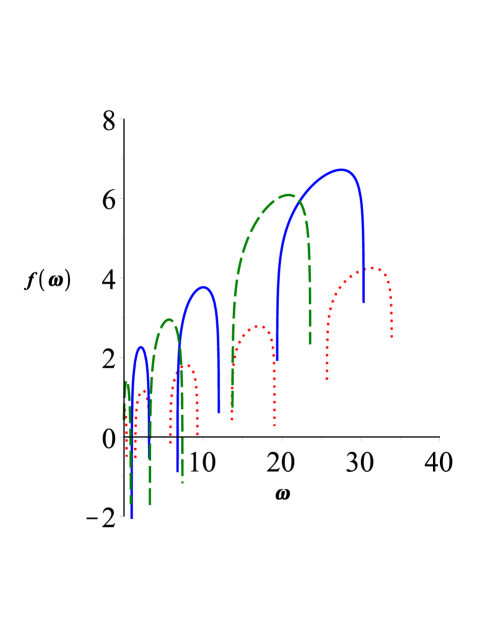
Figure 5: Three different shape functions for the pink noise $(n=-1)$. Solid, dashed and dotted lines are for the parameter sets of $(c_{1}=c_{2}=1;c=1/2,\nu=0.85,\lambda=3,a=2)$, $(c_{1}=c_{2}=1;c=1/2,\nu=0.85,\lambda=2.5,a=2)$, $(c_{1}=c_{2}=1;c=0.6,\nu=0.85,\lambda=5,a=2)$, respectively.

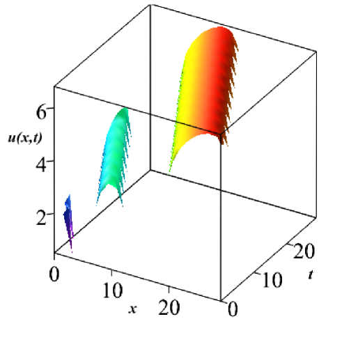
Figure 6: The total solution of the KPZ equation for $n=-1$ with the applied parameter set $c_{1}=c_{2}=1,c=1/2,\nu=0.85\lambda=3$ and $a=2$.

4.3 White noise $n=0$

Here, the noise term is $\eta=a\omega^{0}=a$ which leads to the ODE of

$$-\nu f^{\prime\prime}(\omega)+f^{\prime}(\omega)\left[c-\frac{\lambda}{2}f^{\prime}(\omega)\right]-a=0,$$ (10)

$$f(\omega)=\frac{\omega c}{\lambda}-\frac{\omega\sqrt{c^{2}-2a\lambda}}{\lambda}-\frac{2\nu\ln(2)}{\lambda}-\frac{\nu\ln\left(\frac{c^{2}-2a\lambda}{\lambda^{2}\left[c_{1}e^{\frac{\omega\sqrt{c^{2}-2a\lambda}}{\nu}}-c_{2}\right]^{2}}\right)}{\lambda}$$ (11)

Figure 7 shows two shape functions for two different parameter sets. There exists basically two different functions depending on the ratios of the integral constants $c_{1}$ and $c_{2}$. The first is a pure linear function with infinite range and its domain represents boundless surface growth, which is a physical nonsense. The second solution is a sum of a linear and logarithmic function with a domain bounded from above due to the argument of the $ln$ function. Figure 8 shows the final solution of the KPZ equation $u(x,t)$. We note that with the substitution $\omega=x+ct$ only the first kind of solution remains real. For the second parameter set which creates a modified $ln$ function with a cut at well-defined argument becomes complex.

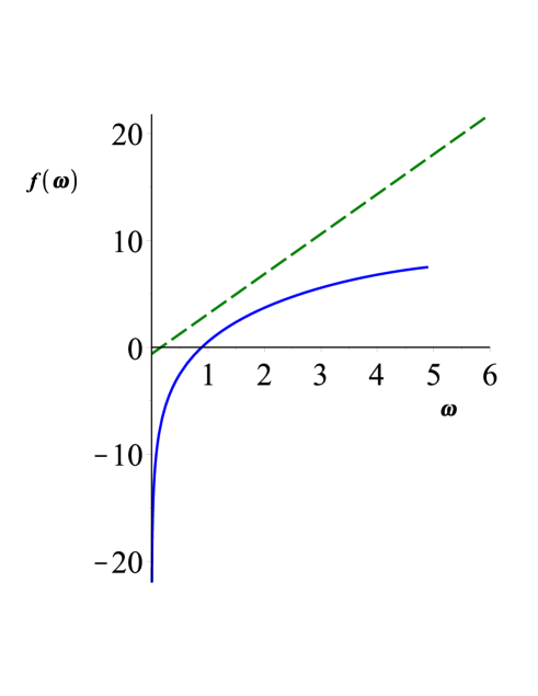
Figure 7: Two shape functions for the constant or white noise. The solid line is for the parameter set $c_{1}=4,\ c_{2}=-1,\ c=0.3,\ \nu=2,\ \lambda=1,\ a=1$, and the dashed line is for $c_{1}=c_{2}=1,\ c=4,\ \nu=0.5,\ \lambda=1,\ a=0.3$, respectively.

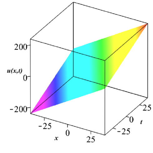
Figure 8: The KPZ solution for the constant or white noise. The applied parameter set is $c_{1}=c_{2}=1,c=4,\nu=0.5,\lambda=1,a=0.3$, respectively.

4.4 Blue noise $n=1$

The last color noise $\eta=a\omega$ leads to the ODE of

$$-\nu f^{\prime\prime}(\omega)+f^{\prime}(\omega)\left[c-\frac{\lambda}{2}f^{\prime}(\omega)\right]-a\omega=0,$$ (12)

with the general solution of

$$f(\omega)=\frac{c\omega}{\lambda}-\frac{4\nu\ln(2)}{3\lambda}+\frac{2\nu}{3\lambda}\ln\left\{\frac{\lambda^{2}[c_{1}Ai(\tilde{\omega})-c_{2}Bi(\tilde{\omega})]^{3}}{\nu a[Ai(1,\tilde{\omega})Bi(1,\tilde{\omega})-Bi(1,\tilde{\omega})Ai(\tilde{\omega}))]^{3}}\right\}$$ (13)

where $Ai(\tilde{\omega}),Bi\tilde{\omega})$ denote the Airy functions of the first and second kind and $Ai(1,\tilde{\omega})$ and $Bi(1,\tilde{\omega})$ are the first derivatives of the Airy functions, where we used the following notation: $\tilde{\omega}=\frac{-(2a\omega\lambda-c^{2})4^{\frac{1}{3}}\left(\frac{a\lambda}{\nu^{2}}\right)^{1/3}}{4a\lambda}$. Exhaustive details of the Airy function can be found in [31]. When the argument $\omega$ is positive, $Ai(\omega)$ is positive, convex, and decreasing exponentially to zero, while $Bi(\omega)$ is positive, convex, and increasing exponentially. When $\omega$ is negative, $Ai\omega)$ and $Bi\omega)$ oscillate around zero with ever-increasing frequency and ever-decreasing amplitude.

Figure 9 represents shape functions with different parameter sets. Our analysis showed that the composite argument of the $ln$ function is purely real having a decaying oscillatory behavior with alternatively positive and negative values. The $ln$ function creates infinite number of separate "bumps" or islands with compact supports and infinite first spatial derivatives at their boarders. Combining the first two terms of the (13), we get an infinite series of separate islands with increasing height. The ratio $c/\lambda$ is the steepness of the line, this automatically defines the steepness of the absolute height of the islands. The effects of the various parameters are not quite independent and hard to define, we may say that in general each parameter $\nu,\lambda,a,c$ alone can change the widths, spacing and absolute height of the peaks. Figure 10 shows the total solution of the KPZ equation. The traveling "bumps" are clearly visible.

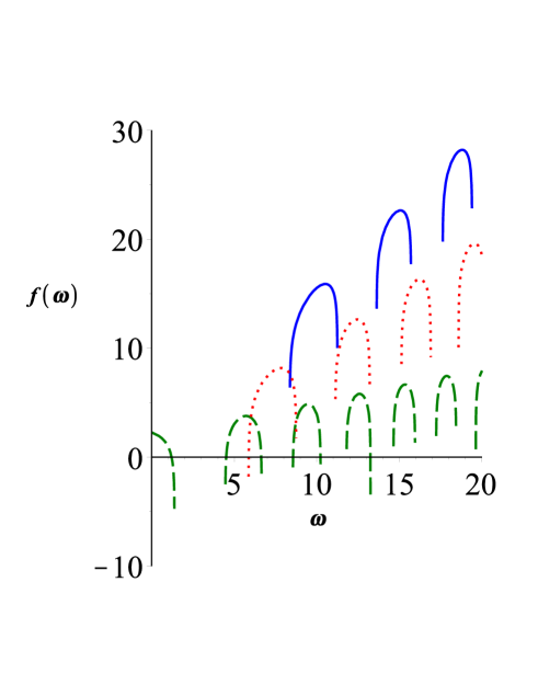
Figure 9: The shape function for the blue noise for three parameter sets. The solid, dashed and dotted lines are for the parameter sets $(c_{1}=1,c_{2}=0,c=3,a=0.5,\nu=1.5,\lambda=2)$ , $(c_{1}=c_{2}=c=1,a=1,\nu=1,\lambda=3)$ , and $(c_{1}=c_{2}=c=1,a=1,\nu=1,\lambda=3)$ , respectively.

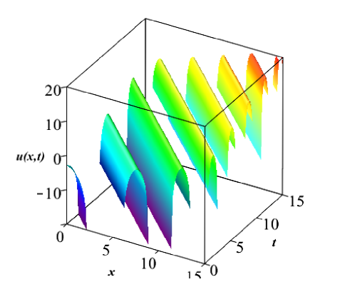
Figure 10: The solution $u(x,t)$ for the $n=1$ or blue noise with the applied parameter set of $c_{1}=c_{2}=c=1,\nu=2,\lambda=3,a=1$

4.5 Lorentzian noise

As a first non-colour noise let us consider the Lorentzian noise of the form $\eta=\frac{a}{1+\omega^{2}}$. It leads to the ODE of

$$-\nu f^{\prime\prime}(\omega)+f^{\prime}(\omega)\left[c-\frac{\lambda}{2}f^{\prime}(\omega)\right]-\frac{a}{1+\omega^{2}}=0,$$ (14)

We mention, that for the classical exponential and Gaussian noise distributions we could not give solutions in closed analytic form. Unfortunately, there is no closed analytic expression available if all the parameters $(\nu,\lambda,c,a)$ are free. The formal solution contains integrals of the Heun C confluent functions multiplied by some polynomials. However, if the parameters $a,\lambda,\nu$ are fixed, there is analytic solution available for free propagation speed $c$. The exact solution for $a=\lambda=\nu=1/2,$ and $c=2$ is the following

$$f(\omega)=c\omega+$$

$$2\ln\left\{\frac{c_{1}C(B)-c_{2}\omega C(A)}{2(\omega^{4}+\omega^{2})[C(A)C^{\prime}(B)-C(B)C^{\prime}(A)]+(1+\omega^{2})C(A)C(B)}\right\},$$ (15)

where $C^{\prime}()$ means the first derivative of the Heun C function. For the better transparency we introduce the following notations $A=0,\frac{1}{2},1,\frac{c^{2}}{4},1-\frac{c^{2}}{4};-\omega^{2}$ and $B=0,-\frac{1}{2},1,\frac{c^{2}}{4},1-\frac{c^{2}}{4};-\omega^{2}$.

Figure 11 shows the shape function for given parameter set. There is a broad island close to the origin and numerous tiny ones at larger arguments. The numerical accuracy of Maple 12 was enhanced to reach this resolution. It is well-known that the Heun functions are the most complicated objects among special functions and the evaluations needs more computer time.

Figure 12 presents the total solution of the original KPZ. Due to the substitution $\omega=x+ct$ the original local solution broke down to several smaller islands which freely propagate in time and space.

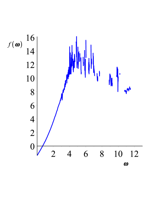
Figure 11: The shape function for the Lorentzian noise. The applied parameters are $c_{1}=0.5,c_{2}=2,c=1,\nu=1,a=1,\lambda=3,$

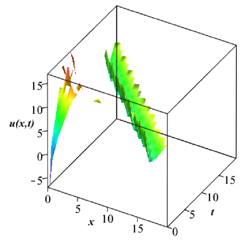
Figure 12: The solution of the KPZ equation for Lorentzian noise, with the parameters mentioned above.

4.6 Periodic noise

The last perturbation investigated is a periodic function $\eta=a\sin(\omega)$ and

$$-\nu f^{\prime\prime}(\omega)+f^{\prime}(\omega)\left[c-\frac{\lambda}{2}f^{\prime}(\omega)\right]-a\sin(\omega)=0.$$ (16)

The general solution can be given as

$$f(\omega)=\frac{1}{\lambda}\left(c\omega+2\ln\left\{\frac{\lambda[c_{1}C(\epsilon_{a})-c_{2}S(\epsilon_{a})]}{\nu[-C^{\prime}(\epsilon_{a})S(\epsilon_{a})+C(\epsilon_{a})S^{\prime}(\epsilon_{a})]}\right\}\right),$$ (17)

where $C(\epsilon_{a}),S(\epsilon_{a}),C^{\prime}(\epsilon_{a})$ and $S^{\prime}(\epsilon_{a})$ are the Mathieu S and Mathieu C functions and the first derivatives. For basic properties we refer to [30]. For a complex study about Mathieu functions see [32, 33, 34]. In (17), we used the abbreviation of $\epsilon_{a}=-\frac{c^{2}}{\nu^{2}},-\frac{a\lambda}{\nu^{2}},-\frac{\pi}{4}+\frac{\omega}{2}$.

Figure 13 shows a typical shape function for the periodic noise term. Due to the elaborate properties of even the single Mathieu C or S functions for some parameter pairs $a,q$ the function is finite with periodic oscillations and for some neighboring parameters it is divergent for large arguments. No general parameter dependence can be stated. The parameter space of the set of six real values $(c_{1},c_{2},c,a,\nu,\lambda)$ is too large to map. After the evaluation of numerous shape functions we may state, that a typical shape function is presented with two larger islands close to the origin and numerous smaller intervals. For large argument $\omega$ the shape function shows a steep decay.

Figure 14 shows the complete solution. Note, that the first two broader islands can be seen as they freely travel. Due to the finite resolution the smaller islands are represented as irregular noise in the background.

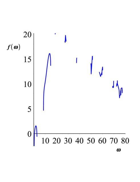
Figure 13: The shape function for the periodic noise. The applied parameters are $c_{1}=0.5,c_{2}=2,c=1,\nu=1,a=1,\lambda=3,$

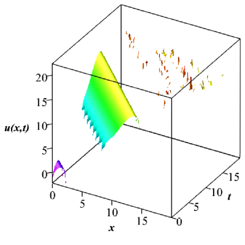
Figure 14: The complete traveling wave solution $u(x,t)$ for periodic noise with the same parameter set as given above.

5 Conclusions

In summary, we can say that with an appropriate change of variables applying the self-similar Ansatz one may obtain analytic solution for the KPZ equation for one spatial dimension with numerous noise terms. We investigated four type of power-law noise $\omega^{n}$ with exponents of $-2,-1,0,1$, called the brown, pink, white and blue noise, respectively. Each integer exponent describes completely different dynamics. Additionally, the properties of Gaussian and Lorentzian noises are investigated. Providing completely dissimilar surfaces with growth dynamics. All solutions can be described with non-trivial combinations of various special functions, like error, Whittaker, Kummer or Heun. The parameter dependencies of the solutions are investigated and discussed. Future works are planned for the investigations of two dimensional surfaces.

References

- [1] A. Pimpinelli and J. Villain. Physics of Crystal Growth. Cambridge University Press, 1998.
- [2] G. Parisi M. Kardar and Yi-C. Zhang. Dynamic scaling of growing interfaces. Phys. Rev. Lett., 56:889, 1986.
- [3] A.-L. Barabási and H. E. Stanley. Fractal concepts in surface growth. Press Syndicate of the University of Cambridge, 1995.
- [4] T. Hwa and E. Frey. Exact scaling function of interface growth dynamics. Physical Review A, 44(12):R7873, 1991.
- [5] E. Frey, U. C. Täuber, and T. Hwa. Mode-coupling and renormalization group results for the noisy burgers equation. Physical Review E, 53(5):4424, 1996.
- [6] M. Lässig. On growth, disorder, and field theory. Journal of physics: Condensed matter, 10(44):9905, 1998.
- [7] T. Kriecherbauer and J. Krug. A pedestrian’s view on interacting particle systems, kpz universality and random matrices. Journal of Physics A: Mathematical and Theoretical, 43(40):403001, 2010.
- [8] M. Matsushita, J. Wakita, H. Itoh, I. Rafols, T. Matsuyama, H. Sakaguchi, and M. Mimura. Interface growth and pattern formation in bacterial colonies. Physica A: Statistical Mechanics and its Applications, 249(1-4):517–524, 1998.
- [9] Y. Kuramoto and T. Tsuzuki. Persistent propagation of concentration waves in dissipative media far from thermal equilibrium. Progress of theoretical physics, 55(2):356–369, 1976.
- [10] G. I. Sivashinsky. Large cells in nonlinear marangoni convection. Physica D: Nonlinear Phenomena, 4(2):227–235, 1982.
- [11] R. Kersner and M. Vicsek. Travelling waves and dynamic scaling in a singular interface equation: analytic results. Journal of Physics A: Mathematical and General, 30(7):2457–2465, 1997.
- [12] T. Sasamoto and H. Spohn. One-dimensional kardar-parisi-zhang equation: an exact solution and its universality. Physical review letters, 104(23):230602, 2010.
- [13] J. Kelling, G. Ódor, and S. Gemming. Suppressing correlations in massively parallel simulations of lattice models. Computer Physics Communications, 220:205–211, 2017.
- [14] T. Martynec and S. H. L. Klapp. Impact of anisotropic interactions on nonequilibrium cluster growth at surfaces. Phys. Rev. E, 98:042801, Oct 2018.
- [15] D. Sergi, A. Camarano, J. M. Molina, A. Ortona, and J. Narciso. Surface growth for molten silicon infiltration into carbon millimeter-sized channels: Lattice–boltzmann simulations, experiments and models. International Journal of Modern Physics C, 27(06):1650062, 2016.
- [16] B. A. Mello. A random rule model of surface growth. Physica A: Statistical Mechanics and its Applications, 419:762–767, 2015.
- [17] Brian H Gilding and Robert Kersner. Travelling waves in nonlinear diffusion-convection reaction, volume 60. Birkhäuser, 2012.
- [18] Mark C Cross and Pierre C Hohenberg. Pattern formation outside of equilibrium. Reviews of modern physics, 65(3):851, 1993.
- [19] Wim Van Saarloos. Front propagation into unstable states. Physics reports, 386(2-6):29–222, 2003.
- [20] Ji-Huan He and Xu-Hong Wu. Exp-function method for nonlinear wave equations. Chaos, Solitons & Fractals, 30(3):700–708, 2006.
- [21] Ismail Aslan and Vangelis Marinakis. Some remarks on exp-function method and its applications. Communications in Theoretical Physics, 56(3):397, 2011.
- [22] Nouredine Benhamidouche. Exact solutions to some nonlinear pdes, travelling profiles method. Electronic Journal of Qualitative Theory of Differential Equations, 2008(15):1–7, 2008.
- [23] L. I. Sedov. Similarity and dimensional methods in mechanics. CRC press, 1993.
- [24] I. F. Barna. Self-similar solutions of three-dimensional navier—stokes equation. Communications in Theoretical Physics, 56(4):745, 2011.
- [25] IF Barna and Laszlo Mátyás. Analytic self-similar solutions of the oberbeck–boussinesq equations. Chaos, Solitons & Fractals, 78:249–255, 2015.
- [26] I. F. Barna. Self-similar analysis of various navier-stokes equations in two or three dimensions. In D. Campos, editor, Handbook on Navier-Stokes Equations, Theory and Applied Analysis, New York, 2017. Nova Publishers.
- [27] Eberhard Hopf. The partial differential equation ut+ uux= xx. Communications on Pure and Applied mathematics, 3(3):201–230, 1950.
- [28] Julian D Cole. On a quasi-linear parabolic equation occurring in aerodynamics. Quarterly of applied mathematics, 9(3):225–236, 1951.
- [29] Imre Ferenc Barna, Gabriella Bognár, Mohammed Guedda, Krisztián Hriczó, and László Mátyás. Analytic self-similar solutions of the kardar-parisi-zhang interface growing equation with various noise term. arXiv preprint arXiv:1904.01838, 2019.
- [30] W. J. F. Olver, D. W. Lozier, R. F. Boisvert, and C. W. Clark. NIST handbook of mathematical functions hardback and CD-ROM. Cambridge University Press, 2010.
- [31] Olivier Vallée and Manuel Soares. Airy functions and applications to physics. World Scientific Publishing Company, 2004.
- [32] Norman W McLachlan. Theory and application of mathieu functions. 1951.
- [33] Josef Meixner and Friedrich Wilhelm Schäfke. Mathieusche Funktionen und Sphäroidfunktionen: mit Anwendungen auf physikalische und technische Probleme, volume 71. Springer-Verlag, 2013.
- [34] F. M. Ascott. Periodic Differential Equations. Pergamon Press, Oxford, 1964.