Comparison of the deep atmospheric dynamics of Jupiter and Saturn in light of the Juno and Cassini gravity measurements

Abstract

The nature and structure of the observed east-west flows on Jupiter and Saturn has been one of the longest-lasting mysteries in planetary science. This mystery has been recently unraveled due to the accurate gravity measurements provided by the Juno mission to Jupiter and the Grand Finale of the Cassini mission to Saturn. These two experiments, which coincidentally happened around the same time, allowed determination of the vertical and meridional profiles of the zonal flows on both planets. This paper reviews the topic of zonal jets on the gas giants in light of the new data from these two experiments. The gravity measurements not only allow the depth of the jets to be constrained, yielding the inference that the jets extend roughly 3000 and 9000 km below the observed clouds on Jupiter and Saturn, respectively, but also provide insights into the mechanisms controlling these zonal flows. Specifically, for both planets this depth corresponds to the depth where electrical conductivity is within an order of magnitude of 1 S m^-1, implying that the magnetic field likely plays a key role in damping the zonal flows.

1 Introduction

The most prominent features in the appearance of Jupiter and Saturn are their east-west banding, which have been observed ever since the invention of the first telescopes in the 17th century. These so called ’zones’ (bright regions) and ’belts’ (dark regions) are related to the two gas giants’ east-west jet-streams. The exact interplay between these zonal flows and the banded structure of the clouds is not completely understood (see recent review by Fletcher et al., 2019), yet the eastward (westward) jets are typically accompanied by a zone to the south (north) and a belt to the north (south). Jupiter has about six distinct jets in each hemisphere (Fig. 1), including a wide superrotating eastward jet around the equator and narrower jets poleward. The strongest jet, reaching $140$ m s^-1 is at latitude $23^{\circ}$N, and is not accompanied by a similar jet in the southern hemisphere, creating a hemispherical asymmetry (Fig. 1). On Saturn, the winds are stronger, with a wider equatorial eastward flow (up to latitude $\sim 30{}^{\circ}$) reaching velocities of nearly $400$ m s^-1. Poleward of that, Saturn has 3-4 distinct jets in each hemisphere (Fig. 1). These jet velocities, measured by cloud tracking (e.g., García-Melendo et al., 2011; Tollefson et al., 2017) and typically quoted relative to Jupiter and Saturn’s magnetic field rotation, have been overall very consistent since the first spacecraft observations in the 1970s. As Saturn’s magnetic field is almost perfectly axisymmetric, this reference frame has a larger uncertainty for the case of Saturn, although recent measurements and theoretical calculations have limited the rotation period uncertainty to within a few minutes (Read et al., 2009; Helled et al., 2015; Mankovich et al., 2019).

Prior to the recent Juno and Cassini missions there have been very little data regarding the flows beneath the cloud tops. The only in-situ measurements come from the Galileo probe, which descended in 1995 into Jupiter’s atmosphere around latitude $6.5^{\circ}$N, and found that the zonal wind velocity increased from around $80$ m s^-1 at the cloud level, where the probe entered, to $\sim 160$ m s^-1 at a depth of 4 bars, and from there downward the zonal velocity remained nearly constant down to $21$ bars (130 km) where the probe was lost (Atkinson et al., 1996). This indicated that the zonal flow was not restricted to the cloud-level, although the depth where it was lost is only a mere fraction of the planetary radius, and thus this measurement did not provide definitive tests to separate between theories suggesting the flows are a shallow atmospheric phenomena (e.g., Williams, 1978, 1979; Cho and Polvani, 1996), and theories suggesting the surface flows are just a surface manifestation of deep cylindrical columns extending deep into the planetary abyss (e.g., Busse, 1976; Heimpel et al., 2005). On Saturn, Cassini observations indicate that low-latitude winds seem to be stronger at the 2-3 bar level than at the cloud-level (0.5 bar), while mid-latitude winds seem to be nearly constant or weaker with depth (Choi et al., 2009; Studwell et al., 2018). Above the cloud layer, tracking wind velocities is difficult as the wind shear can only be indirectly inferred based on temperature measurements (Simon-Miller et al., 2006; Fletcher et al., 2007). Generally for both planets it seems that winds decay above the cloud-level but these measurements are very uncertain (Sánchez-Lavega et al., 2019).

The question of how deep the observed jets extend has been debated extensively in the literature since the early observations by the Pioneer and Voyager missions in the 1970s. Particularly, the research has split into two different approaches for how to explain the jets. According to the first approach, the jets are suggested to be a shallow atmospheric feature, as appears on a terrestrial planet, thus assuming all the dynamics are limited to a shallow weather-layer. Geostrophic turbulence theory provides good understanding to what sets the jet width and overall number of jets (Rhines, 1975; Held and Larichev, 1996; Chemke and Kaspi, 2015), and matches the numbers observed on Jupiter and Saturn. There have been many shallow-type models which have showed formation of jets similar to those on Jupiter and Saturn beginning with the models of Williams (1978, 1979), and over the years evolved to more complex models showing formation of multiple jets (e.g., Panetta, 1993; Vallis and Maltrud, 1993; Cho and Polvani, 1996; Huang and Robinson, 1998; Lee, 2004; Smith, 2004; Showman, 2007; Kaspi and Flierl, 2007; Scott and Polvani, 2007). These shallow-type models most commonly do not exhibit superrotation, but with particular configurations of bottom drag, internal heating, moist convection or thermal damping they can produce an equatorial superrotating jet and multiple high latitude jets (Scott and Polvani, 2008; Lian and Showman, 2008, 2010; Liu and Schneider, 2010; Warneford and Dellar, 2014; Young et al., 2019; Spiga et al., 2020). The second approach considers deep convection models, in which the source of the jets is suggested to be internal convection columns that interact to form the jets seen at the surface. These ideas have also emerged in the 1970s with the seminal papers of Busse (1970, 1976), and evolved to more complex interior convention 3D simulations (e.g., Busse, 1994; Sun et al., 1993; Christensen, 2001; Aurnou and Olson, 2001; Wicht et al., 2002; Heimpel et al., 2005; Kaspi et al., 2009; Jones and Kuzanyan, 2009; Heimpel et al., 2016). These models naturally exhibit superrotation driven by the convergence of convectively driven momentum near the equator, but do not naturally produce the multiple jet structure that appears at the higher latitudes. These two approaches have been debated greatly over the past several decades, but due to the lack of observational evidence, the debate has remained unresolved (see reviews by Vasavada and Showman, 2005 and Showman et al., 2018). Now, following the Juno and Cassini gravity measurements (Iess et al., 2018, 2019), which are reviewed here, the discussion about the source and structure of the jets can be reinvigorated by these new evidence.

Figure 1: The zonal wind profile of Jupiter (left) and Saturn (right), divided in the bottom panels into the north-south symmetric (black) and asymmetric (orange) parts. In the top panels the zonal wind profile for Jupiter (Tollefson et al., 2017) is overlaid on a image taken by the Hubble Wide Field Camera in 2014, and for the Saturn case the zonal wind profile (García-Melendo et al., 2011) is overlaid on an image created by Björn Jónsson by combining Cassini and Voyager images and removing the rings. The grid in both images has a 20^∘ latitudinal spread and a $45^{\circ}$ longitudinal spread. The scale of the zonal flows for Jupiter is the same as the longitudinal grid on the sphere and for Saturn it is triple.

The Juno gravity experiment is one of the key objectives of the Juno mission (Bolton, 2005), with the purpose of measuring Jupiter’s gravity spectra to high accuracy, and thereby providing information about Jupiter’s interior and atmospheric flows (Hubbard, 1999; Kaspi et al., 2010). Juno has been in orbit around Jupiter since July 2016, orbiting Jupiter every 53 days with X and Ka-band radio links to Earth allowing measurements of Jupiter’s gravity field via Doppler shifts in the radio frequencies sent to Earth (Bolton et al., 2017). The measurements are obtained around the time of closest approach (perijove) at 4000 km above the cloud level (Iess et al., 2018). The perijoves are designed to give an overall 360^∘ longitudinal coverage of Jupiter’s as the planet rotates underneath the orbiting spacecraft. In addition, due to the oblateness of Jupiter the perijoves drift about 1^∘ in latitude poleward every orbit, with the first being at latitude $3^{\circ}$N. As the Juno microwave radiometer and the Ka-band radio experiment can not operate in tandem only a subset of the orbits have been devoted to gravity. Nonetheless, there have been enough gravity orbits to date that the error estimate of the measured zonal harmonics has reached saturation.

Motivated by the Juno mission polar orbital configuration, it was decided that during the Cassini Grand Finale (the final Cassini orbits before terminating the mission by a decent into Saturn), the spacecraft would be sent into a polar orbit similar to that of Juno, diving between the planet and the innermost ring with close, 3500-km flybys (Edgington and Spilker, 2016). Between May and August 2017, Cassini performed 22 such flybys (every 6 days), out of which six were devoted for gravity science. Similar to the case of Jupiter, these gravity measurements have allowed the measurement of Saturn’s gravity spectrum up to $J_{10}$, and increased the accuracy of the known harmonics by more than two orders of magnitude (Iess et al., 2019).

In light of these two monumental new experiments, this paper provides a comparative review of what was learned from the gravity measurements regarding the atmospheric and interior dynamics on Jupiter and Saturn. In section 2 we briefly review the dynamical relations connecting the momentum and gravity fields. In section 3 we review the gravity measurements and compare the measured fields on both Jupiter an Saturn. The interpretation of these results in terms of the resulting vertical and meridional profile of the zonal flows that best matches the gravity measurements is shown in section 4. In section 5 we discuss the implications of the commonalities between the Juno and Cassini results, and on what these imply about the possible mechanisms that affect the flow at depth and how the flow might interact with the magnetic field. In section 6 we discuss similar gravity constraints for the zonal flows on Uranus and Neptune, and we conclude in section 7.

2 Theory

The theoretical starting point for understanding the zonal jet dynamics are the Euler equations in the rotating frame

$$\left(\mathbf{u\cdot\nabla}\right)\mathbf{u}+2\Omega\times\mathbf{u}+\Omega\times\left(\Omega\times\mathbf{r}\right) = -\frac{1}{\rho}\nabla p+\nabla V,$$ (1)

where $\mathbf{u}$ is the 3D velocity vector, $\rho$ is density, $p$ is pressure and $V$ is the body force. The rotation rate of Jupiter is given by the System III rotation (Riddle and Warwick, 1976; May et al., 1979), with $\Omega=1.75\times 10^{-4}$ corresponding to a period of $9.92$ hours. For Saturn there has been significant uncertainty in its rotation rate due to the axisymmetric nature of the planets’s magnetic field, but recent studies, using gravity measurements, have constrained the rotation period to $10.57\pm 0.03$ hours (Helled et al., 2015; Mankovich et al., 2019). As both giant planets are rapid rotators, for the purpose of studying the large scale zonal flows, the Rossby number, which is the ratio of the inertial accelerations (first term on lhs in Eq. 1) and the Coriolis accelerations (second term on lhs in Eq. 1), is small. Thus, in the limit of small Rossby number, the fluid is in geostrophic balance (Pedlosky, 1987), meaning:

Figure 2: The measured zonal gravity harmonics of Jupiter and Saturn divided between the even harmonics (red) and odd harmonics (green). For reference the rigid-body harmonics calculated by the CMS model (Hubbard, 1999, 2012) are shown as well (gray). Full circles denote positive values on the log scale and open circles denote negative values. The lines are the Juno and Cassini measurement $3\sigma$ uncertainty (Iess et al., 2018).

$$2\Omega\times\rho\mathbf{u} = -\nabla p-\rho\mathbf{g^{*}},$$ (2)

where $\mathbf{g^{*}}$ is the effective gravitational field, $\mathbf{g^{*}}=-\nabla V+\Omega\times\left(\Omega\times\mathbf{r}\right)$, with the second term being the centrifugal acceleration. Multiplying equation 2 by the density $\rho$, and taking its curl gives

$$2\Omega\cdot\nabla\left(\rho\mathbf{u}\right)=\nabla\rho\times\mathbf{g^{*}},$$ (3)

where the left hand side (lhs) has been simplified using mass conservation $\nabla\cdot\left(\rho\mathbf{u}\right)=0$ and since the rotation rate vector is constant. This also implies that $\mathbf{g^{*}}$ can be expressed as a scalar potential meaning that $\nabla\times\mathbf{g^{*}}=0$, which has been used for the rhs of Eq. 3. This thermal-wind like relation (Kaspi et al., 2009) is different from the standard thermal-wind used in atmospheric science for a shallow atmosphere (e.g., Vallis, 2006), in that the derivatives on the lhs are in the direction of the spin axis and not in the radial direction (the latter is an approximation that holds when the planetary aspect ratio between the vertical and horizontal scales is small), and the rhs involves the full density and effective gravity. Thus, this is a general expression applicable for a rotating atmosphere at any depth as long as the Rossby number is small.

A considerable simplification to this equation can be taken by assuming spherical symmetry. Without this assumption the rhs will involve several terms coming from the deviation of gravity from radial symmetry (both due to the planetary oblateness and dynamical contributions to the gravity vector) and the centrifugal terms (see Eq. 7). In Galanti et al. (2017) and Kaspi et al. (2018) a careful treatment of all these terms is taken, and it is shown that to leading order Eq. 3 is given by

$$2\Omega\cdot\nabla\left(\rho_{s}\mathbf{u}\right)=\nabla\rho^{\prime}\mathbf{\times}\mathbf{g_{s}},$$ (4)

where $\rho$ has been split into static $\rho_{s}\left(r\right)$ and dynamical $\rho^{\prime}\left(r,\theta\right)$ components, $r$ is the radial direction and $\theta$ is latitude. Here $\mathbf{g_{s}}$ is the radial gravitational acceleration coming from integrating $\rho_{s}$. It is important to note that if the spherical assumption is not taken in Eq. 3 the rhs evolves into several different terms of equal magnitude (Galanti et al., 2017), and using only part of them (Zhang et al., 2015) leads to an inconsistent expansion (see more detail below). Since the flows on the giant planets are predominantly in the zonal direction, taking the zonal components of Eq. 4 allows integrating the flow induced density gradient to give the dynamical contribution to the gravity harmonics given by

$$\Delta J_{n}=-\frac{2\pi}{Ma^{n}}\intop_{-1}^{1}d\mu\intop_{0}^{R\left(\mu\right)}r^{n+2}P_{n}\left(\mu\right)\rho^{\prime}\left(r,\mu\right)dr,$$ (5)

where $M$ is the planetary mass, $a$ is the planetary mean radius, $R$ is the 1-bar radius, $P_{n}$ are the associated Legendre polynomials and $\mu=\sin\left(\theta\right).$ Note that when integrating $\frac{\partial\rho^{\prime}}{\partial\theta}$ from the zonal component of Eq. 4, for use in Eq. 5, an undetermined radially dependent integration function arrises $\left(\rho^{\prime}_{0}\left(r\right)\right)$. However such a function will not project onto the gravity harmonics when multiplied by the $P_{n}$ in Eq. 5, since

$$\intop_{-1}^{1}d\mu\intop_{0}^{a}r^{n+2}P_{n}\left(\mu\right)\rho^{\prime}_{0}\left(r\right)dr=0,$$ (6)

because the latitudinally dependent associated Legendre polynomials $P_{n}$ have a zero mean. Therefore in spherical geometry the dynamical gravity anomalies can be uniquely determined, despite the density anomaly itself being determined only up to an unknown constant of integration (Kaspi et al., 2016).

There has been debate in the literature whether an additional term, namely $\nabla\rho_{s}\times\mathbf{g^{\prime}}$ which appears to be of the same order as the rhs of Eq. 4 should be included in that equation (termed the thermal-gravity wind equation by Zhang et al., 2015). However, this additional term contains a deviation from radial symmetry and therefore it was dropped going from Eq. 3 to Eq. 4. If this term is retained, then for consistency, other terms that involve deviation from radial symmetry, and are of the same order from Eq. 3, must to be retained as well (Galanti et al., 2017). Then the azimuthal component of Eq. 3 will take the form:

$$2\Omega\frac{\partial}{\partial z}\left(\rho_{s}u\right)=\frac{g_{s}^{(r)}}{r}\frac{\partial\rho^{\prime}}{\partial\theta}-g_{s}^{(\theta)}\frac{\partial\rho^{\prime}}{\partial r}+\frac{g^{\prime(r)}}{r}\frac{\partial\rho_{s}}{\partial\theta}-g^{\prime(\theta)}\frac{\partial\rho_{s}}{\partial r}+\Omega^{2}\left[\frac{\partial\rho^{\prime}}{\partial\theta}\cos^{2}\theta+\frac{\partial\rho^{\prime}}{\partial r}r\cos\theta\sin\theta\right],$$ (7)

where $u$ is the velocity component in the azimuthal direction, and the notation $\frac{\partial}{\partial z}\equiv\cos\theta\frac{1}{r}\frac{\partial}{\partial\theta}+\sin\theta\frac{\partial}{\partial r}$ denotes the derivative along the direction of the axis of rotation. Note that in the radial symmetric limit the rhs reduces to only the first term on the rhs which is exactly the azimuthal component of Eq. 4 giving thermal-wind balance. Eq. 7 is an integro-differential equation since both the gravity $\mathbf{g_{s}}$ and $\mathbf{g^{\prime}}$, are calculated by integrating $\rho_{s}$ and $\rho^{\prime}$, respectively. Although this equation can be solved numerically (Galanti et al., 2017), the additional terms (terms 2-6 on the rhs) are all small and contribute very little to the gravity solution. The individual contribution of each of the terms in Eq. 7 is shown in Kaspi et al. (2018) for the case of Jupiter, demonstrating that the first term on the rhs is indeed the leading order term. All other terms in this equation are at least an order of magnitude smaller, meaning that taking $\mathbf{g}=\mathbf{g}\left(r\right)$ and neglecting the centrifugal terms gives the leading order solution. Galanti et al. (2017) solves the full equation 7 and shows that the resulting gravity harmonics are very close to those resulting from using thermal wind balance. Other solutions, such as retaining only the first and third terms on the rhs of Eq. 7 (Zhang et al., 2015; Kong et al., 2018), are thus inconsistent and invalid.

3 The Juno and Cassini gravity measurements

Table 1: Values of Jupiter’s $J_{2}-J_{10}$ gravity harmonics. Measured values are the Juno measured values with the uncertainty being three times the formal uncertainty (Iess et al., 2018). The interior model values with no dynamics are averages from the ensemble of rigid-body interior models presented in Guillot et al. (2018). The dynamical contribution is the difference between the measured values and the rigid-body models with no dynamics. The fifth column shows the dynamical solutions when using the cloud-level profile of the zonal winds (Fig. 1), extend down along the direction of the spin axis with a best fit e-folding decay value of $H=1471$ km (Eq. 8). The sixth column shows the solutions when using the cloud level winds, but with a more complex decay function as described in Kaspi et al. (2018). The seventh column shows the solutions when optimizing both the meridional and vertical profile of zonal wind (as shown in Fig. 5, blue), with the optimization done for the odd gravity harmonics only (as for columns 5 and 6). The last column shows the same but optimizing for the even gravity harmonics as well (the profiles are shown in Fig. 5, green). The last row shows the normalized rms of the difference between the measurements and the solution for all cases, giving a relative value for how close the solution is to the measurements.

The close orbits of Juno and Cassini yielded determination of the gravity harmonics of Jupiter and Saturn to unprecedented accuracy (Iess et al., 2018, 2019). Prior to these missions, the only known gravity harmonics were $J_{2}$, $J_{4}$ and $J_{6}$ (Jacobson, 2003; Jacobson et al., 2006). Supplementary Fig. 1 illustrates how much these have been improved over the last few decades showing the significant reduction in the uncertainty going from the Voyager era to the Juno and Cassini measurements. In addition, the higher-order even harmonics $J_{8}$ and $J_{10}$ have been now determined with high accuracy as well (Tables 1 and 2). These even harmonics are mostly affected by the interior density distribution and shape of the planet, and only to second order by the flow ($\Delta J_{n}$, Eq. 5), although the relative contribution from the flow grows for the higher harmonics and becomes of similar order to that associated to the rotational flattening beyond $J_{10}$ (Hubbard, 1999). Conversely, the odd gravity harmonics ($J_{3},$ $J_{5}$, $J_{7}$ etc.) have no contribution from the interior static density distribution and shape as these are purely north-south symmetric for such gas planets. The only possible contribution to the odd gravity harmonics comes from asymmetries in the dynamics (see the asymmetry in the wind profiles of both Jupiter and Saturn in Fig. 1). Therefore, in terms of probing the dynamics using gravity measurements, the odd harmonics provide a more direct way of determining the depth of the flows (Kaspi, 2013).

The values of the even harmonics are to leading order powers of $q^{n}$, where $q$ is the ratio of the gravity to centrifugal terms in Eq. 1 (Hubbard, 1984). The rotation therefore is dominant is determining the values in the rigid-body limit (no dynamics) in addition to the internal density distribution. The dependence on the density distribution is more complex, and can be calculated by internal models (e.g., Hubbard, 1975; Hubbard and Marley, 1989; Hubbard, 1999, 2012; Nettelmann et al., 2012; Miguel et al., 2016; Hubbard and Militzer, 2016), and depends on the equation of state (EOS) as well (e.g., Militzer and Hubbard, 2013; Chabrier et al., 2019). Both the interior models and the EOS are topics of intense research and will not be reviewed here, as the focus is on the dynamics. Most pre Juno/Cassini published interior structure models for Jupiter and Saturn gave gravity harmonics outside of the narrow range of the Juno and Cassini measurements (Supplementary Fig. 1), resulting in a need for improving the interior models and EOSs. The first to match the Juno measurements to an internal model was Wahl et al. (2017), who found that the Juno measured harmonics can only be matched if Jupiter has a dilute core that expands to a significant fraction of the planet’s radius. These results, however, heavily depend on the choice of EOS. Recently, Debras and Chabrier (2019) presented a new model for the interior of giant planets, and were able to match with a new EOS the Juno measurements as well as the abundance of heavy elements measured by Galileo. Their results also support the existence of an extended diluted core enriched by heavy elements.

Despite the dynamical contribution to the even gravity harmonics being small relative to the rotation and interior mass distribution, due to the high accuracy of the Juno and Cassini gravity measurements the dynamical effects on the even harmonics turned to be larger than the formal measurement uncertainty (supplementary Fig. 1). Therefore, without any knowledge of how much mass is involved in the flow (i.e., how deep the flows are), the dynamical effects can be regarded as the effective uncertainty of the gravity harmonics (Kaspi et al., 2017; Debras and Chabrier, 2019). In Supplementary Fig. 1 we show this effective uncertainty considering a wide range of possible flow profiles calculated using the method described in section 2 and assuming no a priori knowledge about the internal dynamics (i.e., before the Juno and Cassini measurements). However, given the current knowledge about how deep the cloud-level flows are, and assuming there are no other significant internal flows that affect the even harmonics, allows more accurate estimates of the effective uncertainty where the dynamical correction to the measurements of the even harmonics is already taken into account. In Supplementary Fig. 1 we show both the effective uncertainty assuming no knowledge on the dynamical contribution (yellow shading), and the dynamical contribution given the knowledge of the flow depth (green dots). For Jupiter, the odd harmonics allowed getting an independent measure of the flow depth without need to use the even harmonics; while for Saturn, as discussed in section 4, the even harmonics are needed to determine the flow depth which makes this effective uncertainty more ambiguous.

Table 2: Values of Saturn’s $J_{2}-J_{10}$ gravity harmonics. Measured values are the Cassini Grand Finale measured values with the uncertainty being three times the formal uncertainty (Iess et al., 2019). The model values without dynamics are the average values from the ensemble of models presented in Galanti et al. (2019). The dynamical contribution is the difference between the measured values and the rigid-body models with no dynamics. The fifth column shows the solutions when using the cloud-level profile of the zonal winds (Fig. 1), and extending them along the direction of the spin axis with a best-fit e-folding decay value of $H=12995$ km (Eq. 8). The sixth column shows the solutions when using the cloud level winds, but with a more complex decay function as described in Galanti et al. (2019). The seventh column shows solutions when optimizing both the meridional and vertical profile of zonal wind (as shown in Fig. 5, green) with the optimization done for the even and odd gravity harmonics together (as for columns 5 and 6). The last column shows the same, but optimizing for the odd harmonics only (the profiles are shown in Fig. 5, blue). The last row shows the normalized standard deviation of the difference between the measurements solution for all cases, giving a relative value for how close the solution is to the measurements.

The measured even gravity harmonics by Juno and Cassini, as well as theoretical estimates for the gravity values if Jupiter and Saturn were rotating as a rigid body (equivalent to a case where the dynamics are very shallow and have no influence on the gravity field) are presented in Fig. 2 (red and gray dots, respectively). The numerical values for Jupiter and Saturn are presented as well in Tables 1 and 2, respectively. As expected, the low order even harmonics match previous estimates as they are mostly dominated by non-dynamical effects, and thus very close to the rigid body values. For Jupiter, also $J_{8}$ and $J_{10}$ are relatively close to the rigid-body values and therefore the measured even harmonics and the rigid-body values are virtually indistinguishable in Fig. 2. However, for the Saturn case, these values differ substantially, indicating that the flows are deeper than on Jupiter. This separation between the measurements and the rigid-body values matches Hubbard (1999)’s prediction that if a planet is differentially rotating the even gravity harmonics beyond $n=8$ will differ from the rigid-body theoretical values. Hubbard’s solution allowed only for cases of full differential rotation, meaning the surface flows extend throughout the whole planet (i.e., following the Busse, 1976 barotropic model). Intermediate cases for which the surface flows halt at a certain depth can be obtained using methods as presented in section 2 (Kaspi et al., 2010). Quantitative solutions showing which vertical decay profiles best match these measurements are presented in section 4.

A key result of the gravity measurement was that the measured odd gravity harmonics vary significantly from zero. The measured values (green dots in Fig. 2), match predicted theoretical values (Kaspi, 2013) calculated by extending the observed cloud-level wind inward along the direction of the spin axis and calculating their affect on the gravity field (see section 4). The fact that the expected gravity signal of zonal flows was in fact detected, confirmed that dynamics play a role in redistributing mass inside the planet and that the dynamics are deep enough to affect the measured gravity field. Different from the even gravity harmonics, the odd harmonics have no contribution from the non-dynamical interior mass distribution as it should not have any north-south asymmetries on a gas planet. The observed jets on the other hand do have north-south asymmetries (Fig. 1) and are the only considerable source of north-south asymmetries on the gravity field. Other sources of north-south asymmetries can be internal oscillations (Durante et al., 2017) and the known north-south asymmetry in the magnetic field (Connerney et al., 2018; Moore et al., 2018). However, internal oscillations can be expected to give fluctuating contributions from orbit to orbit whereas the measured odd harmonics are steady. The magnetic effect can be expected to scale as the ratio of magnetic pressure to total pressure. For a field of $100$ Gauss (plausibly the unobserved toroidal field) in a region of total pressure of $\sim 100$ kilobars (at $\sim 0.96$ Jupiter radii), this is of order $3\times 10^{-9}$, likely too small to be important, although it cannot be excluded with complete certainty because this field (unlike the observed poloidal field) is not known. For the case of Jupiter, $J_{3}$, $J_{5}$, $J_{7}$ and $J_{9}$ were measured to be above the 3-sigma uncertainty level (black line in Fig. 2), while for Saturn only the first two are above the 3-sigma uncertainty level. The robustness of the odd harmonics measurement of Jupiter allowed therefore to uniquely determine the depth and structure of the flow even without consideration of the even harmonics. For the case of Saturn, this turned to be more complex, because only the first two odd gravity harmonics are above the uncertainty level, and as shown below those alone do not give a solution that matches the even harmonics as well.

4 Inversion of the gravity fields into wind fields

Given the measurements from Juno and Cassini, the challenge is to translate these measurements into the wind fields that generate them. The challenge is both in the conversion between the gravity anomaly data and the dynamically balanced wind field, and in dealing with the non-unique nature of such solutions. Given that the gravity field is described by only a finite set of values (Fig. 2), while a full wind field will require many degrees of freedom to describe properly, it is obvious that the solution is not unique, and the more degrees of freedom the wind field has, the easier it will be to find a fit to the gravity data. We present therefore here a hierarchal approach beginning with a simple case where the wind is described with only one degree of freedom, meaning a greater number of observables (the gravity harmonics), and then present cases with more degrees of freedom for the wind profile allowing better matches to the gravity data, but never allow more degrees of freedom for the wind than the number of overall observables.

Figure 3: Theoretical values of the even (top) and odd (bottom) gravity harmonics as function of the e-folding depth ($H$) of the cloud-level wind profile for Jupiter (left) and Saturn (right). The solid curves are the predicted dynamical contributions to $J_{n}$ (Kaspi, 2013), for winds decaying exponentially from the measured cloud-top winds given an e-folding depth $H$. The horizontal dashed lines are the measured values from Juno and Cassini, where for the even harmonics the rigid-body values used in Tables 1 and 2 have been subtracted. Depth values that match the corresponding measured gravity harmonics correspond to locations where the solid curve crosses the dashed line of the same color.

We begin with a simple forward model in which we assume the observed cloud-level flow at the 1 bar level decays radially towards the interior with an e-folding depth defined as $H$. This represents the expectation that the wind will overall decay with depth (despite possible enhancement at the high levels as measured by the Galileo probe), due to the compressibility of the fluid and/or Ohmic dissipation at depth due to increasing electrical conductivity. Due to the dominance of rotation, the cloud-level flow is extended inward along the direction of the spin axis, but the decay itself is radial since the density growth inward is also radial, meaning the functional dependence of the zonal flow is given by

$$u\left(r,\theta\right)=u_{{\rm cyl}}\left(r,\theta\right)\exp\left[\left(r-a\right)/H\right],$$ (8)

where $u_{{\rm cyl}}$ is the cloud-level wind profile extended inward along the direction of the axis of rotation and $H$ is the e-folding radial decay height of this flow (the other parameters are as defined in section 2). Such simplified models for the wind profile have been used in several studies (Kaspi et al., 2010; Kaspi, 2013; Liu et al., 2013; Kaspi et al., 2016; Kong et al., 2016; Guillot et al., 2018).

Given such a zonal wind profile, Eq. 4 can be used to generate the density anomaly gradients that balance this flow profile, and the dynamical gravity harmonics (Eq. 5) can be obtained. Fig. 3 (solid lines) shows such calculated gravity harmonics as function of the e-folding depth of the flow as predicted in Kaspi (2013), for both the even gravity harmonics (top) and the odd harmonics (bottom). Note that the values of all harmonics switch sign as function of depth depending on how the integrated density structure that is balancing the wind projects on the different spherical harmonics. Although the sign of these values is not intuitive—the overall tendency to larger values with depth is—due to having more mass involved with the flow. The measured values from Juno and Cassini are shown (dashed lines) on top of the theoretical prediction curves. For the even harmonics, $\Delta J_{n}$ is calculated as the difference between the measurements and the average rigid-body values from an ensemble of interior models (Guillot et al., 2018; Galanti et al., 2019; see Tables 1 and 2).

For the Jupiter case, the measured odd harmonics are all negative except $J_{7}$ which is positive, matching the prediction for this simplified model for depths of several thousand kilometers (indicated by the crossing between the solid and dashed lines in Fig. 3). Note that all the four gravity harmonics, independently, match the Kaspi (2013) prediction by sign and indicate that the depth of the flow is between 1000 and 3000 kilometers, with the optimized best fit e-folding depth for all harmonics combined being $H=1471$ km. Furthermore, the even gravity harmonics (omitting $J_{2}$ and $J_{4}$ where the relative contribution of the dynamics is very small) show a similar result where all three theoretical curves cross the measurement value between depths of 1500 and 2000 km. The fact that for all seven values ($J_{3}$ and $J_{5}$-$J_{10}$), the theoretical calculation matches the Juno measurement in sign and value gives a strong indication that the observed cloud-level flow is related to these measured gravity anomalies and indicates their depth. Nonetheless, using an exponential decay law for the cloud-level winds does not give an exact match to the gravity data (Table 1, column 5), and indeed exponential decay with a uniform e-folding depth was not made based on physical reasoning but for simplicity. Below we present more complex decay functions which better match the measurements, yet the simple model’s overall match to the data gives a strong indication to the relation between the observed flows, their depth and the gravity measurements.

Optimizing for a more complex decay function we use an adjoint based inversion technique (Galanti and Kaspi, 2016), where a cost function is minimized to give a best fit between the decay profile and the gravity measurements, taking into account the uncertainties in the gravity measurements and the error covariance between the different harmonics (Kaspi et al., 2018). Solutions for the vertical decay functions using this method with three degrees of freedom for the shape of the vertical profile (see Kaspi et al., 2018 for details) are shown in Fig. 4. Taking the exact observed cloud-level zonal flows and extending them into the interior with this best optimized vertical decay function gives a much better match to the gravity data than the exponential decay function (Table 1, column 6). Next, allowing the optimization procedure to include small variations to the cloud-level wind profile (assuming the zonal wind meridional profile at depth may vary somewhat from what is observed at the cloud-level) shows that in this case the solutions give an even better match (Table 1, column 7) to all 4 measured odd gravity harmonics (note that even harmonics are not optimized here, but still give a rather good match). Fig. 4 shows that in this case the variations to the observed wind profiles are very minor and well within the uncertainty (and observed variation between the Voyager and Juno eras) of this profile. The vertical profile in this case (blue) is very similar to the one obtained without varying the meridional structure of the wind profile indicating again the decay being at around several thousand kilometers.

As the odd harmonics are a consequence of the dynamics alone we have used only them so far for the optimization procedure. Despite this, the resulting even $\Delta J_{n}$ for these vertical profiles match well both in sign and in magnitude the difference between the measurements of $J_{6}$, $J_{8}$ and $J_{10}$ and the rigid body values (compare columns 4 and 7 in Table 1). Thus it is clear that if we include the even values in the optimization the results will not differ substantially. In the final column of Table 1 we present such an optimization, where now all values of the seven gravity harmonics ($J_{3}$ and $J_{5}$-$J_{10}$) match exactly the measurements. Here again we allow the wind profile to vary from the observed wind structure, though as can be seen in Fig. 4 the wind profile needs very minor changes in order to match the gravity measurements perfectly. We emphasize though that this exercise is not unique and other meridional and vertical profiles of the zonal flow can give an exact match to the gravity data. However, following Occam’s razor reasoning, here we have shown that taking the observed cloud-level flow, and extending it inward in a very simple fashion gives an exact match to the gravity measurements.

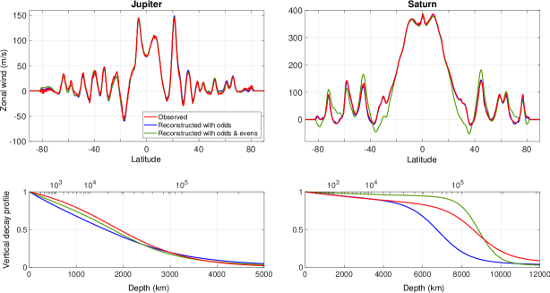
Figure 4: The optimized meridional profile (top) of the zonal wind for Jupiter (left) and Saturn (right), comparing the observed cloud-level profile (red), the optimized best fit solutions taking into account the odd harmonics only (blue), and the optimized best fit solutions taking into account both the odd and even harmonics (green). The resulting gravity harmonic values for these profiles appear in Tables 1 and 2. The bottom panel shows the corresponding vertical structures of the zonal flow as function of depth (km) and pressure (bar).

Complementary to this analysis, Guillot et al. (2018) used a wide range of rigid-body models for Jupiter (without averaging as in Table 1, column 3) to construct the possible dynamical contribution range to the even zonal harmonics, by subtracting this range of rigid-body solutions from the Juno gravity measurements. This range was used to constrain a wide range of hypothetical flow profiles derived using thermal wind balance (as in Kaspi et al. (2017)), not bounded to the observed cloud-level flows with different e-folding decay depths. This analysis, consistent with the analysis presented above, showed that with high likelihood the flow extends down to $2000-3500$ km beneath the cloud-level. Although the Guillot et al. (2018) analysis is not sensitive to provide the vertical decay profile of the flow, nor can it constrain the meridional profile of the zonal flow, it gives an independent method for constraining the bulk depth of the flow using the even gravity harmonics alone. Given the match of the flow to the even gravity harmonics it also indicates that the flow beneath this layer is likely very weak ($<5$ m s^-1), otherwise it would have an influence on the measured even gravity harmonics.

For the Saturn case, the cloud-level flow has shown much more variability between the Voyager and the Cassini eras (García-Melendo et al., 2011), and is more uncertain. Repeating the same analysis as for the Jupiter case and taking the cloud-level flow with a simple exponential decay gives a relatively good match to the even harmonics (same sign and within factor of 2 in magnitude) for e-folding depths of $\sim 10^{4}$ km. This indicates a substantially deeper flow than for the case of Jupiter. The odd harmonics for the Saturn case, despite being not very different in magnitude than for Jupiter, are closer to the measurement uncertainty and therefore only $J_{3}$ and $J_{5}$ have significant values (Fig. 2). Both, however, give an opposite sign compared to the theoretical prediction when using the cloud-level wind profile, indicating that a more sophisticated model is needed for Saturn. Similarly, as long as using the cloud-level winds, taking a more complex decay profile does not give a good match to the gravity measurements (Table 2, column 6). However, when allowing the cloud level wind to deviate from the observed profile, a good match to the measurements can be found (Fig. 4, green profile).

The deviation from the observed wind profile of Saturn is mainly around latitude 30^∘ where the flow needs to be more westward than the observed cloud-level wind, with values $\sim 50$ m s^-1 in order to match the measurements for both the even and odd harmonics (Table 2, column 7). The match is obtained with a vertical profile which is nearly barotropic down to $\sim 8000$ km and then decays with depth (green profile in Fig. 4) (Galanti et al., 2019). A similar conclusion, that a westward flow around latitude 30^∘ is needed in order to match the even gravity harmonics, was also reached by Militzer et al. (2019) who used a model allowing the flow to extend inward only barotropically (without changing along the direction of the spin axis), and found that such a westward zonal flow profile (but twice as large) is needed to match the measurements. Based on theoretical argument alone, Chachan and Stevenson (2019) obtained a similar conclusion that a retrograde wind profile is necessary around latitude 30^∘ in order to match the measurements. The optimizations discussed here used both the values of the odd and the even harmonics and took into account all cross correlations. For the case of Saturn, optimizing with odd harmonics only does not give a good match to the even harmonics, highlighting the difference between Jupiter and Saturn and pointing to that for Saturn the high order even harmonics (particularly $J_{8}$ and $J_{10}$) are key to determine the depth and profile of the deep flows. The uncertainty in rotation rate affects only the dynamical $J_{2}$ and $J_{4}$ and thus is not important for interpreting the Saturn gravity measurements (Galanti and Kaspi, 2017).

Comparing the different columns in Tables 1 and 2 and considering the different profiles in Fig. 5 shows that the gravity results not only inform us about the depth of the jets, but also about the meridional profile of the zonal flow at depth. The results show that the measurements are sensitive to the exact meridional profile, although the variations to it needed to get exact matches are not significant. To test the statistical significance of this profile, other profiles with a different meridional profile of the zonal flow have been tested, to investigate the possibility that the flow at depth might exhibit major qualitative differences from the flow observed at cloud-level. Out of a sample of a thousand zonal-wind profiles as a function of latitude with the same overall amplitude but different meridional profile, less than 1% had a better match to the measurements using the same optimization procedure (Kaspi et al., 2018). These few profiles had no correlation to one another, nor to the cloud-level profile. This indicates that although such random solutions can be found, it is with high confidence that the same meridional profile of the zonal flow that is observed at the surface extends to depth.

5 Interaction of the flow with the magnetic field at depth

The results presented above have shown some key similarities and differences between Jupiter and Saturn. On both planets, the measured gravity harmonics indicate how deep the cloud-level flows extend, and give a good match to a zonal wind profile at depth being very similar to the one observed at the cloud-level of both planets. Differently, on Jupiter the jets extend down to $\sim 3000$ km while on Saturn that depth nearly triples (Fig. 5). However, note that the mass of Jupiter is $3.3$ times that of Saturn while the radius is only about $1.2$ times larger, resulting in the fact that the gravitational acceleration on Jupiter is about three times larger than that of Saturn. As a result, the electrical conductivity of Saturn only achieves large values at a much greater depth than it does on Jupiter (Fig. 5 red dashed lines in the top panels). Despite the different depth, note that in both cases the rise in electrical conductivity is near $10^{5}$ bar, due to the dependence of electrical conductivity on temperature (Stevenson, 2003). Strikingly, the depth where the electrical conductivity rises in both planets is at the same depth where the gravity measurements imply that the zonal winds decay (where the blue and red curves cross in Fig. 5). This strongly hints that Ohmic dissipation plays a role in damping the flow at depth, and in fact was predicted previously based on theoretical arguments (Liu et al., 2008; Cao and Stevenson, 2017).

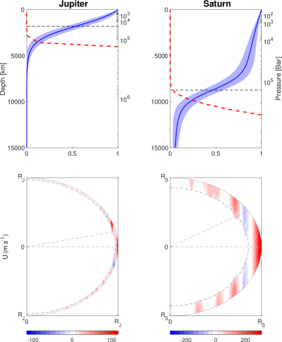
Figure 5: The vertical structure of the zonal flow on Jupiter (left) and Saturn (right) as function of depth corresponding to the best fit profile presented in column 6 of Table 1 and column 7 of Table 2, respectively. The upper panel shows this vertical profile function (blue), its uncertainty (blue shading) and the electrical conductivity profile (red dashed) as given by Liu et al. (2008) for Jupiter and French et al. (2012) for Saturn. The electrical conductivity is in units of S m^-1 with the scale going linearly from 0 to 100. The middle point in the decay profile, at depths of $1831$ km and $8743$ km for Jupiter and Saturn, respectively, is marked by the dashed horizontal line. The bottom panels show the same zonal flow profile as function of latitude and depth in the spherical projection. The middle point corresponding to that shown in the upper panels appears as the thick dashed line. The thin dashed lines contain the angle (latitude) derived from extending the depth of the flow along the direction of the spin axis ($\theta_{e}=\cos^{-1}\left(x/a\right)$, where $a$ is the planetary radius and $x$ is the depth beyond the middle point of the flow profile). This latitude ($\theta_{e}$) is $13^{\circ}$ for Jupiter and $31^{\circ}$ for Saturn, close to the latitude where the flow is observed to turn from eastward to westward at the cloud-level.

As a consequence, the depth at which a particular pressure is reached in Saturn is about three times greater than the corresponding depth for Jupiter. The temperature at a given pressure is only modestly ($\sim 20\%$) lower in Saturn than in Jupiter. Temperature is most important for determining the electrical conductivity of hydrogen, which results from excitation of electrons across the band gap between valence and conduction states (Stevenson and Salpeter, 1977). This conductivity is an extremely strong function of temperature, both in theoretical (French et al., 2012) and experimental results (Nellis et al., 1992), which are essentially in agreement. The expected conductivity at 3000 km in Jupiter and 9000 km in Saturn (about $10^{5}$ bars in both planets) is approximately 1 S m^-1 (similar to that of salty water at room temperature). At this conductivity, strong zonal winds would create a toroidal magnetic field whose associated electrical currents would produce a total Ohmic dissipation that is comparable to the observed luminosity of the planets (Liu, 2006; Liu et al., 2008).

The factor of three difference in zonal wind depth between Jupiter and Saturn, together with a remarkable correspondence to the theoretical argument of (Liu et al., 2008) (their prediction was $2800$ km for Jupiter) strongly suggests the role of magnetohydrodynamics. It should also be noted that because the electrical conductivity is such an extremely strong function of temperature and therefore radius, the results hold even given a likely order of magnitude uncertainty in the electrical conductivity and the large difference in field strengths between Jupiter and Saturn. Some cautionary comments are in order, however: first, the argument is purely kinematic; that is, there is as yet no fully dynamical argument that explains this truncation of the flows by the magnetic field. Moreover, the Lorentz force is not sufficient by itself to dampen the flows from large values (tens of m s^-1) to zero (Cao and Stevenson, 2017). Clearly the role of the magnetic field is more complicated and the full solution to the zonal flow requires an understanding of the spatial structure of the deviation from constant entropy throughout the envelope (Eq. 9).

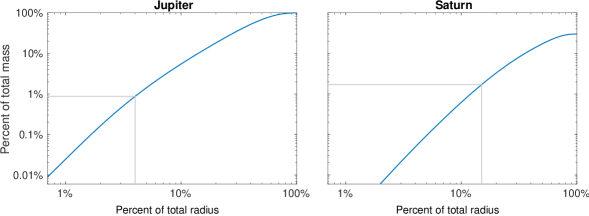
Figure 6: The percentage of Jupiter (left) and Saturn’s (right) mass as a function of depth beneath the 1-bar level. The grey line shows that percentage of mass contained within the depth of the zonal flows as found by the gravity measurements.

Therefore, although the Ohmic dissipation might be ultimately what halts the flow at depth, it does not explain what diminishes the strength of the flow substantially from the cloud-level down to where the electrical conductivity becomes large (Fig. 5). In this region the dissipation of the zonal flow needs to be due to other mechanisms. Reorganization of Eq. 4, looking at its zonal component and assuming the background profile is adiabatic leads to a relation between the wind shear along the direction of the spin axis and the entropy gradients (Kaspi et al., 2009):

$$\frac{\partial u}{\partial z} = -\frac{g}{2\Omega\rho_{s}}\left(\frac{\partial\rho}{\partial s}\right)_{p}\frac{1}{r}\frac{\partial s^{\prime}}{\partial\theta}$$ (9)

where $s$ is entropy. Thus the direction of the shear is determined by the average sign of the entropy gradients, and the shear is expected to be largest at the lower depths where the density is smallest. Note that in the purely barotropic limit, the rhs of equation vanishes leading to the flow being purely aligned with the axis of rotation. This is similar to the Taylor-Proudman theorem (Pedlosky, 1987), only that the Taylor-Proudman theorem requires the fluid to be incompressible, in which case all three components of velocity are aligned with the rotation axis ($2\Omega\cdot\nabla\mathbf{u}=0$ ). For a compressible flow, in the barotropic limit, the alignment is for the zonal and meridional component of the flow (throughout this paper only the zonal component of the velocity is discussed). Yet, due to the entropy gradients (Eq. 9), and as evident from the gravity results, the flow is likely not fully barotropic (baroclinic). Quantitatively however, the shear on both planets is of O(100 m s^-1) over thousands of kilometers, implying that the flows in effect are not very far from barotropic. If, for example, we assume the variation from barotropic is very large and allow the observed flows to extend inward in a different way (e.g., radially) the match to the gravity measurements would not have been as good as it is here (Tables 1, 2). For example, extending the cloud-level flow inward radially for Jupiter results in $J_{3}$ changing sign. Only if the zonal flow meridional profile is altered substantially solutions can be found.

An additional question regarding the zonal flows is the issue of their forcing mechanism. It is well understood from terrestrial atmospheric dynamics that geostrophic turbulence on a rotating planet will drive turbulent eddy momentum fluxes resulting in regions of momentum flux convergence with eastward (prograde) flows and momentum flux divergence with westward (retrograde) flows. It has been observed for Jupiter (Salyk et al., 2006) and Saturn (Del Genio et al., 2007) that indeed there is a strong correlation between the regions of eddy momentum flux convergence (divergence) and the eastward (westward) jets, implying this is a plausible mechanism for driving the zonal flows. Yet, it is not known what is the source of the eddies, with candidates being barotropic or baroclinic instabilities (e.g., Kaspi and Flierl, 2007) or the internal convection itself. It has also been shown that both shallow and deep forcing can drive such zonal flows (Showman et al., 2006). The driving and dissipation mechanisms discussed here can be seen in a single expression by taking the leading component of the momentum equation (Eq. 1) and expressing it in terms of angular momentum (Vallis, 2006). Taking a zonal and vertical average and in steady state gives, $\mathbf{u}\cdot\nabla M=-S+D$ , where $M$ is angular momentum, $S$ is the eddy momentum flux divergence and $D$ is the Lorentz drag (Schneider and Liu, 2009). In regions of low electrical conductivity, closer to the cloud-level, the balance will be $\mathbf{u}\cdot\nabla M=-S$ with the momentum flux providing the cross angular momentum surfaces (i.e., across the direction of the spin axis) flux to force eastward momentum flux convergence and zonal jets. In the the deep region, where the electrical conductivity is high, the drag allows for cross angular momentum flow, $\mathbf{u}\cdot\nabla M=D$, to close the circulation. In between, $\mathbf{u}\cdot\nabla M=0$, meaning there is no cross angular momentum flow and the flow must be aligned with the direction of axis of rotation. Note though that this has no implication on how barotropic is the zonal flow, and this argument puts a strong constraint on the meridional circulation but not on the zonal flow itself. These arguments are similar to those used to explain the midlatitude Ferrel cell on Earth with surface drag taking the place of the Lorentz drag (Vallis, 2006).

The dynamical constraints discussed earlier suggest that the flow likely extends inward along the direction of the spin axis as demonstrated in Fig. 5 where the full solution for the zonal wind in the radial-latitudinal plane is presented. It is evident that for the case of Jupiter, despite the jets being deep from an atmospheric perspective, extending down to 10⁵ bars and advecting 1% of the mass of the whole planet (Fig. 6), from the point of view of the whole gaseous planet, and compared to the proposed Busse (1976) model scenario, the winds penetrate only a small fraction of the planet. For Saturn, the fraction is larger, going down to 15% of the radius of the planet, but still containing only a few percent of the total mass (Fig. 6). That said, on both planets, the atmospheric advection of several percent of the planetary mass is very significant, and by far extends the advection on every other planet in the solar system (e.g., Earth’s atmosphere is less than one part in a million of the planetary mass).

Note that the depth for both Jupiter and Saturn obtained from the gravity measurements is also consistent with the observed latitudinal extent of the equatorial eastward flow; meaning that if the depth of the flow at the equator is extended along the direction of the axis of rotation, it interests the surface almost exactly at the latitude where the zonal flow turns from positive to negative (eastward to westward). Quantitatively, taking the half point of the flow depth (horizontal lines in the top panels of Fig. 5), being $1831$ km for Jupiter and $8743$ km for Saturn, and calculating the latitude where this line intersects the surface gives a latitude of $13^{\circ}$ for Jupiter and $31^{\circ}$ for Saturn. This is very close to the latitude where the equatorial flow changes sign which is $13^{\circ}$ and $35^{\circ}$ for Jupiter and Saturn, respectively. Note that for the Saturn case if a rotation rate of 10:34 is taken instead of 10:39 as recent publications indicate this latitude changes to $31^{\circ}$ (Fig. 1). Thus, this gives another independent observation which is in agreement with the conclusion from the gravity measurements regarding the depth of the zonal jets. Such arguments regarding the depth of the equatorial superrotation region have been presented in the past in the context of the tangent cylinder surrounding the inner region of deep convective models (e.g., Heimpel et al., 2005; Aurnou et al., 2008; Kaspi et al., 2009; Liu and Schneider, 2010; Gastine et al., 2013).

6 The depth of the zonal flow on Uranus and Neptune

As on Jupiter and Saturn, Uranus and Neptune also have very strong east-west flows at the observed cloud-level. These flows reach $\sim 200$ m s^-1 on Uranus and nearly $400$ m s^-1 on Neptune, with a meridional structure which is overall similar between the two planets, consisting of a westward broad equatorial flow and a strong and broad eastward flow at midlatitudes. The flows have an overall similar character despite the obliquity being very different ($98^{\circ}$ on Uranus and $29^{\circ}$ on Neptune), and the internal heat flux being three times stronger than the solar flux on Neptune while on Uranus the internal heat flux appears to be negligible (Pearl et al., 1990; Pearl and Conrath, 1991). As these are the only two planets yet to host a dedicated space mission (Fletcher et al., 2019), most data comes from the Voyager encounters of the two planets in 1986 and 1989 (Smith et al., 1986, 1989). The data obtained from Voyager includes the gravity harmonics up to $J_{4}$, although to a much lesser precision than the Juno and Cassini data discussed above (Jacobson, 2007, 2009). Nonetheless, due to the broader shape of the wind structure and its relative resemblance to the meridional structure of $P_{4}$ (Eq. 5), it was possible to place an upper bound on the depth of the atmospheric circulation on these planets (Kaspi et al., 2013).

This was done utilizing the known values of $J_{4}$ from Voyager and determining the difference between the observed $J_{4}$, and the $J_{4}$ resulting from a wide range of rigid-body models set to match all other observational constraints besides $J_{4}$. Any difference in these quantities places constraints on the dynamical contribution to $J_{4}$. Therefore, considering the observed $J_{4}$ and its uncertainty and the widest possible range of $J_{4}$ solutions from interior models, ranging from models with no solid cores to ones with massive solid cores (Helled et al., 2010, 2011; Nettelmann et al., 2013), an upper limit to the dynamic contribution to $J_{4}$ ($\Delta J_{4}$, as in Eq. 5) was constructed. This revealed that the dynamics are constrained to the outermost 0.4% of the mass on Uranus and 0.2% on Neptune, providing a much stronger limitation to the depth of the dynamical atmosphere than previously suggested (Hubbard et al., 1991). This result implies that the dynamics must be confined to a thin weather layer of no more than 1600 km on Uranus and 1000 km on Neptune (Kaspi et al., 2013). This is much shallower than the depths on Jupiter and Saturn with the pressure to which the flows extends being at most 4000 bar on Uranus and 2000 bar on Neptune.

7 Discussion and Conclusion

The recent gravity measurements of Juno and Cassini have provided data accurate enough to allow inferring the effect of atmospheric dynamics on the gravity field of both planets. This allowed determining the depth of the flows on both planets, and inferring that the meridional profile of the zonal flows observed at the cloud-level of both planets likely extends to depth. An intrinsic problem of any gravity inversion is that the contributing field is not unique, meaning in this case that the wind-induced gravity anomalies can not be traced uniquely to the wind field creating them. However, there are several independent lines of evidence supporting the solutions presented here:

1. The simplest possible Jovian flow model, taking the observed cloud-level winds and extending them inward, matches all 4 measured odd gravity harmonics ($J_{3}$, $J_{5}$, $J_{7}$ and $J_{9}$) independently both in sign and in magnitude (Fig. 3).

2. The same wind profile matches the dynamical component of the even gravity harmonics ($J_{6}$, $J_{8}$ and $J_{10}$) as well (Fig. 3).

3. There are no other likely sources of north-south asymmetries that can match in magnitude the measured values of the odd gravity harmonics (section 5).

4. A statistical analysis taking random zonal wind profiles (considering that the cloud-level winds may be decoupled from the interior flow causing the measured gravity anomalies), shows that less than 1% of such wind profiles give a match to the gravity measurements (Kaspi et al., 2018).

5. The Saturnian winds, with slight modifications (within the error range of the wind measurements), match the dynamical component of the gravity measurements for both the even and odd harmonics (Fig. 4).

6. For both Jupiter and Saturn, the depth of the flows inferred from the gravity measurements matches the depth where electrical conductivity rises abruptly. This suggests that the previously suggested mechanism of Ohmic dissipation might play a key role in setting the flow depth (Liu et al., 2008).

7. For both Jupiter and Saturn, the depth of the flows inferred from the gravity measurements matches the depth inferred from a tangent cylinder separating the equatorial eastward flow and the higher latitude flows. This may explain the different latitudinal extent of the equatorial flow on both planets (Fig. 5).

8. Temporal variation of the magnetic field of Jupiter implies that the variation is carried by the zonal flow and gives a magnitude of the zonal flow at depth consistent with the depth implied by the gravity measurements (Moore et al., 2019).

Overall, although each one of these evidence separately can be perhaps challenged as being coincidental, when taken together, these consistent lines of evidence combined yield a coherent picture regarding the extent and character of the flows beneath the cloud-level of Jupiter and Saturn. On both planets, the flows advect a substantial part of the mass of the planets ($1-2\%$), greater than in any other planetary atmospheres (Fig. 6). This depth implies that the flows span from top to bottom, nearly four orders of magnitude in density and nearly six orders of magnitude in pressure. That said, the depth on both planets is just a small fraction of the planetary radius ($\sim 4\%$ on Jupiter and $\sim 15\%$ on Saturn), suggesting that from a planetary perspective the flows are still bound to a relatively shallow layer.

Despite this new understanding regarding the depth and structure of the flow, we are still left with an incomplete picture of the mechanisms driving the flow. Particularly, several open questions remain, such as what causes the flow to decay before reaching the Ohmic dissipation level at $\sim 10^{5}$ bar? What drives the equatorial superrotation? Why are the flows on Saturn substantially stronger? What are the source of the eddies driving the jets? What are the roles of baroclinic, barotropic and convective instabilities in driving the winds? With better constrains on the dynamical component of the gravity fields (due to improved interior models), magnetic fields and their secular variation (future Juno orbits), temperature fields and water abundance (Juno microwave measurements) and improved dynamical models these questions might be addressed in the coming years, to give a better understanding of the fundamental physical processes driving the dynamics on the giant planets.

Figure 7: Supplementary Figure I: Historical (pre Juno and Cassini) measured values of $J_{2}$, $J_{4}$ and $J_{6}$ and their uncertainty for Jupiter (top) and Saturn (bottom) and the Juno and Cassini measurements (including $J_{8}$, red). Voyager values (purple) are from Campbell and Synnott (1985) for Jupiter and Campbell and Anderson (1989) for Saturn, and Cassini values (black) are from Jacobson (2003) for Jupiter and Jacobson et al. (2006) for Saturn. Recent Juno and Cassini results are from Iess et al. (2018) for Jupiter and Iess et al. (2019) for Saturn. The effective uncertainty due to dynamics assuming no knowledge on the flow and taking the widest possible range of internal flows (see Kaspi et al., 2017 for details) centered around the Juno/Cassini-measured values appears in yellow, with the contour for $H=3000$ km (Jupiter) and $H=10000$ km (Saturn) in dashed. In green is the difference between the recent Juno/Cassini measurement and the best fit flow profile presented in this paper ($J_{n}-\Delta J_{n}$), where $\Delta J_{n}$ is taken from column 7 in Tables 1 and 2 ($\Delta J_{2}$ for Saturn is out of the range presented in that panel), giving our best estimate to what internal models (with no dynamics) should match to.

References

- Atkinson et al. (1996) D.H. Atkinson, J.B. Pollack, A. Seiff, Galileo doppler measurements of the deep zonal winds at Jupiter. Science 272, 842–843 (1996)
- Aurnou and Olson (2001) J.M. Aurnou, P.L. Olson, Strong zonal winds from thermal convectionin a rotating spherical shell. Geophys. Res. Lett. 28(13), 2557–2559 (2001)
- Aurnou et al. (2008) J. Aurnou, M. Heimpel, L. Allen, E. King, J. Wicht, Convective heat transfer and the pattern of thermal emission on the gas giants. Geophysical Journal International 173, 793–801 (2008)
- Bolton (2005) S.J. Bolton, Juno Final Concept Study Report, Technical Report AO-03-OSS-03, New Frontiers, NASA, 2005
- Bolton et al. (2017) S.J. Bolton, A. Adriani, V. Adumitroaie, M. Allison, J. Anderson, S. Atreya, J. Bloxham, S. Brown, J.E.P. Connerney, E. DeJong, W. Folkner, D. Gautier, D. Grassi, S. Gulkis, T. Guillot, C. Hansen, W.B. Hubbard, L. Iess, A. Ingersoll, M. Janssen, J. Jorgensen, Y. Kaspi, S.M. Levin, C. Li, J. Lunine, Y. Miguel, A. Mura, G. Orton, T. Owen, M. Ravine, E. Smith, P. Steffes, E. Stone, D. Stevenson, R. Thorne, J. Waite, D. Durante, R.W. Ebert, T.K. Greathouse, V. Hue, M. Parisi, J.R. Szalay, R. Wilson, Jupiter’s interior and deep atmosphere: The initial pole-to-pole passes with the Juno spacecraft. Science 356, 821–825 (2017)
- Busse (1970) F.H. Busse, Thermal instabilities in rapidly rotating systems. J. Fluid Mech. 44, 441–460 (1970)
- Busse (1976) F.H. Busse, A simple model of convection in the Jovian atmosphere. Icarus 29, 255–260 (1976)
- Busse (1994) F.H. Busse, Convection driven zonal flows and vortices in the major planets. Chaos 4(2), 123–134 (1994)
- Campbell and Anderson (1989) J.K. Campbell, J.D. Anderson, Gravity field of the Saturnian system from Pioneer and Voyager tracking data. Astrophys. J. 97, 1485 (1989)
- Campbell and Synnott (1985) J.K. Campbell, S.P. Synnott, Gravity field of the Jovian system from pioneer and Voyager tracking data. Astrophys. J. 90, 364–372 (1985)
- Cao and Stevenson (2017) H. Cao, D.J. Stevenson, Zonal flow magnetic field interaction in the semi-conducting region of giant planets. Icarus 296, 59–72 (2017)
- Chabrier et al. (2019) G. Chabrier, S. Mazevet, F. Soubiran, A new equation of state for dense hydrogen-helium mixtures. Astrophys. J. 872, 51 (2019)
- Chachan and Stevenson (2019) Y. Chachan, D.J. Stevenson, A linear approximation for the effect of cylindrical differential rotation on gravitational moments: Application to the non-unique interpretation of Saturn’s gravity. Icarus 323, 87–98 (2019)
- Chemke and Kaspi (2015) R. Chemke, Y. Kaspi, The latitudinal dependence of atmospheric jet scales and macroturbulent energy cascades. J. Atmos. Sci. 72, 3891–3907 (2015)
- Cho and Polvani (1996) J. Cho, L.M. Polvani, The formation of jets and vortices from freely-evolving shallow water turbulence on the surface of a sphere. Phys. of Fluids. 8, 1531–1552 (1996)
- Cho and Polvani (1996) J.Y.-K. Cho, L.M. Polvani, The morphogenesis of bands and zonal winds in the atmospheres on the giant outer planets. Science 273, 335–337 (1996)
- Choi et al. (2009) D.S. Choi, A.P. Showman, R.H. Brown, Cloud features and zonal wind measurements of Saturn’s atmosphere as observed by Cassini/VIMS. J. Geophys. Res. (Planets) 114(E4), 04007 (2009)
- Christensen (2001) U.R. Christensen, Zonal flow driven by deep convection in the major planets. Geophys. Res. Lett. 28, 2553–2556 (2001)
- Connerney et al. (2018) J.E.P. Connerney, S. Kotsiaros, R.J. Oliversen, J.R. Espley, J.L. Joergensen, P.S. Joergensen, J.M.G. Merayo, M. Herceg, J. Bloxham, K.M. Moore, A new model of Jupiter’s magnetic field from Juno’s first nine orbits. Geophys. Res. Lett. 45(6), 2590–2596 (2018)
- Debras and Chabrier (2019) F. Debras, G. Chabrier, New models of Jupiter in the context of Juno and Galileo. Astrophys. J. 872, 100 (2019)
- Del Genio et al. (2007) A.D. Del Genio, J.M. Barbara, J. Ferrier, A.P. Ingersoll, R.A. West, A.R. Vasavada, J. Spitale, C.C. Porco, Saturn eddy momentum fluxes and convection: First estimates from Cassini images. Icarus 189(2), 479–492 (2007)
- Durante et al. (2017) D. Durante, T. Guillot, L. Iess, The effect of Jupiter oscillations on Juno gravity measurements. Icarus 282, 174–182 (2017)
- Edgington and Spilker (2016) S.G. Edgington, L.J. Spilker, Cassini’s Grand Finale. Nature Geoscience 9, 472–473 (2016)
- Fletcher et al. (2007) L.N. Fletcher, P.G.J. Irwin, N.A. Teanby, G.S. Orton, P.D. Parrish, R. de Kok, C. Howett, S.B. Calcutt, N. Bowles, F.W. Taylor, Characterising Saturn’s vertical temperature structure from Cassini/CIRS. Icarus 189(2), 457–478 (2007)
- Fletcher et al. (2019) L.N. Fletcher, Y. Kaspi, A.P. Showman, T. Guillot, How well do we understand the belt/zone circulation of Giant Planet atmospheres? Space Sci. Rev. (2019). Submitted
- Fletcher et al. (2019) L.N. Fletcher, N. André, D. Andrews, M. Bannister, E. Bunce, T. Cavalié, S. Charnoz, F. Ferri, J. Fortney, D. Grassi, L. Griton, P. Hartogh, R. Helled, R. Hueso, G. Jones, Y. Kaspi, L. Lamy, A. Masters, H. Melin, J. Moses, O. Mousis, N. Nettleman, C. Plainaki, E. Roussos, J. Schmidt, A. Simon, G. Tobie, P. Tortora, F. Tosi, D. Turrini, Ice giant systems: The scientific potential of missions to Uranus and Neptune (ESA voyage 2050 white paper). arXiv e-prints (2019)
- French et al. (2012) M. French, A. Becker, W. Lorenzen, N. Nettelmann, M. Bethkenhagen, J. Wicht, R. Redmer, Ab initio simulations for material properties along the Jupiter adiabat. Astrophys. J. Sup. 202(1), 5 (2012)
- Galanti and Kaspi (2016) E. Galanti, Y. Kaspi, An adjoint based method for the inversion of the Juno and Cassini gravity measurements into wind fields. Astrophys. J. 820, 91 (2016)
- Galanti and Kaspi (2017) E. Galanti, Y. Kaspi, Prediction for the flow-induced gravity field of Saturn: implications for Cassini’s Grande Finale. Astrophys. J. Let. 843, 25 (2017)
- Galanti et al. (2017) E. Galanti, Y. Kaspi, E. Tziperman, A full, self-consistent, treatment of thermal wind balance on fluid planets. J. Fluid Mech. 810, 175–195 (2017)
- Galanti et al. (2019) E. Galanti, Y. Kaspi, Y. Miguel, T. Guillot, D. Durante, P. Racioppa, L. Iess, Saturn’s deep atmospheric flows revealed by the Cassini grand finale gravity measurements. Geophys. Res. Lett. 46(2), 616–624 (2019)
- García-Melendo et al. (2011) E. García-Melendo, S. Pérez-Hoyos, A. Sánchez-Lavega, R. Hueso, Saturn’s zonal wind profile in 2004-2009 from Cassini ISS images and its long-term variability. Icarus 215(1), 62–74 (2011)
- Gastine et al. (2013) T. Gastine, J. Wicht, J.M. Aurnou, Zonal flow regimes in rotating anelastic spherical shells: An application to giant planets. Icarus 225, 156–172 (2013)
- Guillot et al. (2018) T. Guillot, Y. Miguel, B. Militzer, W.B. Hubbard, Y. Kaspi, E. Galanti, H. Cao, R. Helled, S.M. Wahl, L. Iess, W.M. Folkner, D.J. Stevenson, J.I. Lunine, D.R. Reese, A. Biekman, M. Parisi, D. Durante, J.E.P. Connerney, S.M. Levin, S.J. Bolton, A suppression of differential rotation in Jupiter’s deep interior. Nature 555, 227–230 (2018)
- Heimpel et al. (2005) M. Heimpel, J. Aurnou, J. Wicht, Simulation of equatorial and high-latitude jets on Jupiter in a deep convection model. Nature 438, 193–196 (2005)
- Heimpel et al. (2016) M. Heimpel, T. Gastine, J. Wicht, Simulation of deep-seated zonal jets and shallow vortices in gas giant atmospheres. Nature Geoscience 9, 19–23 (2016)
- Held and Larichev (1996) I.M. Held, V.D. Larichev, A scaling theory for horizontally homogeneous, baroclinically unstable flow on a beta plane. J. Atmos. Sci. 53(7), 946–952 (1996)
- Helled et al. (2010) R. Helled, J.D. Anderson, G. Schubert, Uranus and Neptune: Shape and rotation. Icarus 210, 446–454 (2010)
- Helled et al. (2015) R. Helled, E. Galanti, Y. Kaspi, Saturn’s fast spin determined from its gravitational field and oblateness. Nature 520, 202–204 (2015)
- Helled et al. (2011) R. Helled, J.D. Anderson, M. Podolak, G. Schubert, Interior models of Uranus and Neptune. Astrophys. J. 726, 15 (2011)
- Huang and Robinson (1998) H.P. Huang, W.A. Robinson, Two-dimentional turbulence and persistent jets in a global barotropic model. J. Atmos. Sci. 55, 611–632 (1998)
- Hubbard (1975) W.B. Hubbard, Gravitational field of a rotating planet with a polytropic index of unity. Soviet Astronomy 18, 621–624 (1975)
- Hubbard (1984) W.B. Hubbard, Planetary Interiors (pp. 343. New York, Van Nostrand Reinhold Co., ???, 1984)
- Hubbard (1999) W.B. Hubbard, Note: Gravitational signature of Jupiter’s deep zonal flows. Icarus 137, 357–359 (1999)
- Hubbard (2012) W.B. Hubbard, High-precision Maclaurin-based models of rotating liquid planets. Astrophys. J. Let. 756, 15 (2012)
- Hubbard and Marley (1989) W.B. Hubbard, M.S. Marley, Optimized Jupiter, Saturn, and Uranus interior models. Icarus 78, 102–118 (1989)
- Hubbard and Militzer (2016) W.B. Hubbard, B. Militzer, A preliminary Jupiter model. Astrophys. J. 820, 80 (2016)
- Hubbard et al. (1991) W.B. Hubbard, W.J. Nellis, A.C. Mitchell, N.C. Holmes, P.C. McCandless, S.S. Limaye, Interior structure of Neptune - comparison with Uranus. Science 253, 648–651 (1991)
- Iess et al. (2018) L. Iess, W.M. Folkner, D. Durante, M. Parisi, Y. Kaspi, E. Galanti, T. Guillot, W.B. Hubbard, D.J. Stevenson, J.D. Anderson, D.R. Buccino, L.G. Casajus, A. Milani, R. Park, P. Racioppa, D. Serra, P. Tortora, M. Zannoni, H. Cao, R. Helled, J.I. Lunine, Y. Miguel, B. Militzer, S. Wahl, J.E.P. Connerney, S.M. Levin, S.J. Bolton, Measurement of Jupiter’s asymmetric gravity field. Nature 555, 220–222 (2018)
- Iess et al. (2019) L. Iess, B. Militzer, Y. Kaspi, P. Nicholson, D. Durante, P. Racioppa, A. Anabtawi, E. Galanti, W.B. Hubbard, M.J. Mariani, P. Tortora, W.S. M, M. Zannoni, Measurement and implications of Saturn’s gravity field and ring mass. Science 364, 1052 (2019)
- Jacobson (2003) R.A. Jacobson, JUP230 orbit solutions, 2003. http://ssd.jpl.nasa.gov/
- Jacobson (2007) R.A. Jacobson, The Gravity Field of the Uranian System and the Orbits of the Uranian Satellites and Rings, in AAS/Division for Planetary Sciences Meeting Abstracts #39. Bull. Am. Astro. Soc., vol. 38, 2007, pp. 453–453
- Jacobson (2009) R.A. Jacobson, The orbits of the Neptunian satellites and the orientation of the pole of Neptune. Astrophys. J. 137, 4322–4329 (2009)
- Jacobson et al. (2006) R.A. Jacobson, P.G. Antreasian, J.J. Bordi, K.E. Criddle, R. Ionasescu, J.B. Jones, R.A. Mackenzie, M.C. Meek, D. Parcher, F.J. Pelletier, W.M. Owen Jr., D.C. Roth, I.M. Roundhill, J.R. Stauch, The gravity field of the Saturnian system from satellite observations and spacecraft tracking data. Astrophys. J. 132, 2520–2526 (2006)
- Jones and Kuzanyan (2009) C.A. Jones, K.M. Kuzanyan, Compressible convection in the deep atmospheres of giant planets. Icarus 204, 227–238 (2009)
- Kaspi (2013) Y. Kaspi, Inferring the depth of the zonal jets on Jupiter and Saturn from odd gravity harmonics. Geophys. Res. Lett. 40, 676–680 (2013)
- Kaspi and Flierl (2007) Y. Kaspi, G.R. Flierl, Formation of jets by baroclinic instability on gas planet atmospheres. J. Atmos. Sci. 64, 3177–3194 (2007)
- Kaspi et al. (2009) Y. Kaspi, G.R. Flierl, A.P. Showman, The deep wind structure of the giant planets: Results from an anelastic general circulation model. Icarus 202, 525–542 (2009)
- Kaspi et al. (2010) Y. Kaspi, W.B. Hubbard, A.P. Showman, G.R. Flierl, Gravitational signature of Jupiter’s internal dynamics. Geophys. Res. Lett. 37, 01204 (2010)
- Kaspi et al. (2013) Y. Kaspi, A.P. Showman, W.B. Hubbard, O. Aharonson, R. Helled, Atmospheric confinement of jet-streams on Uranus and Neptune. Nature 497, 344–347 (2013)
- Kaspi et al. (2016) Y. Kaspi, J.E. Davighi, E. Galanti, W.B. Hubbard, The gravitational signature of internal flows in giant planets: comparing the thermal wind approach with barotropic potential-surface methods. Icarus 276, 170–181 (2016)
- Kaspi et al. (2017) Y. Kaspi, E. Galanti, R. Helled, Y. Miguel, W.B. Hubbard, B. Militzer, S. Wahl, S. Levin, J. Connerney, S. Bolton, The effect of differential rotation on Jupiter’s low-degree even gravity moments. Geophys. Res. Lett. 44, 5960–5968 (2017)
- Kaspi et al. (2018) Y. Kaspi, E. Galanti, W.B. Hubbard, D.J. Stevenson, S.J. Bolton, L. Iess, T. Guillot, J. Bloxham, J.E.P. Connerney, H. Cao, D. Durante, W.M. Folkner, R. Helled, A.P. Ingersoll, S.M. Levin, J.I. Lunine, Y. Miguel, B. Militzer, M. Parisi, S.M. Wahl, Jupiter’s atmospheric jet streams extend thousands of kilometres deep. Nature 555, 223–226 (2018)
- Kong et al. (2016) D. Kong, K. Zhang, G. Schubert, A fully self-consistent multi-layered model of Jupiter. Astrophys. J. 826, 127 (2016)
- Kong et al. (2018) D. Kong, K. Zhang, G. Schubert, J.D. Anderson, Origin of Jupiter’s cloud-level zonal winds remains a puzzle even after Juno. Proc. Natl. Acad. Sci. U.S.A. 115(34), 8499–8504 (2018)
- Lee (2004) S. Lee, Baroclinic multiple jets on a sphere. J. Atmos. Sci. 62, 2484–2498 (2004)
- Lian and Showman (2008) Y. Lian, A.P. Showman, Deep jets on gas-giant planets. Icarus 194, 597–615 (2008)
- Lian and Showman (2010) Y. Lian, A.P. Showman, Generation of equatorial jets by large-scale latent heating on the giant planets. Icarus 207, 373–393 (2010)
- Liu (2006) J. Liu, Interaction of magnetic field and flow in the outer shells of giant planets, PhD thesis, California Institute of Technology, 2006
- Liu and Schneider (2010) J. Liu, T. Schneider, Mechanisms of jet formation on the giant planets. J. Atmos. Sci. 67, 3652–3672 (2010)
- Liu et al. (2008) J. Liu, P.M. Goldreich, D.J. Stevenson, Constraints on deep-seated zonal winds inside Jupiter and Saturn. Icarus 196, 653–664 (2008)
- Liu et al. (2013) J. Liu, T. Schneider, Y. Kaspi, Predictions of thermal and gravitational signals of Jupiter’s deep zonal winds. Icarus 224, 114–125 (2013)
- Mankovich et al. (2019) C. Mankovich, M.S. Marley, J.J. Fortney, N. Movshovitz, Cassini ring seismology as a probe of Saturn’s interior. I. rigid rotation. Astrophys. J. 871, 1 (2019)
- May et al. (1979) J. May, T.D. Carr, M.D. Desch, Decametric radio measurement of Jupiter’s rotation period. Icarus 40, 87–93 (1979)
- Miguel et al. (2016) Y. Miguel, T. Guillot, L. Fayon, Jupiter internal structure: the effect of different equations of state. Astron. and Astrophys. 596, 114 (2016)
- Militzer and Hubbard (2013) B. Militzer, W.B. Hubbard, Ab initio equation of state for hydrogen-helium mixtures with recalibration of the giant-planet mass-radius relation. Astrophys. J. 774, 148 (2013)
- Militzer et al. (2019) B. Militzer, S. Wahl, W.B. Hubbard, Models of Saturn’s interior constructed with accelerated concentric maclaurin spheroid method. arXiv e-prints, 1905–08907 (2019)
- Moore et al. (2019) K.M. Moore, H. Cao, J. Bloxham, D.J. Stevenson, J.E.P. Connerney, S.J. Bolton, Time variation of Jupiter’s internal magnetic field consistent with zonal wind advection. Nature Astronomy, 325 (2019)
- Moore et al. (2018) K. Moore, R. Yadav, L. Kulowski, H. Cao, J. Bloxham, J.E.P. Connerney, S. Kotsiaros, J. Jorgensen, J. Merayo, D. Stevenson, S.J. Bolton, L.S. M., A complex Jovian dynamo from the hemispheric dichotomy of Jupiter’s field. Nature 561, 76–78 (2018)
- Nellis et al. (1992) W.J. Nellis, A.C. Mitchell, P.C. McCandless, D.J. Erskine, S.T. Weir, Electronic energy gap of molecular hydrogen from electrical conductivity measurements at high shock pressures. Phys. Rev. Let. 68(19), 2937–2940 (1992)
- Nettelmann et al. (2012) N. Nettelmann, A. Becker, B. Holst, R. Redmer, Jupiter models with improved Ab initio hydrogen equation of state (H-REOS.2). Astrophys. J. 750, 52 (2012)
- Nettelmann et al. (2013) N. Nettelmann, R. Helled, J.J. Fortney, R. Redmer, New indication for a dichotomy in the interior structure of Uranus and Neptune from the application of modified shape and rotation data. Planatary and Space Science (2013)
- Panetta (1993) R.L. Panetta, Zonal jets in wide baroclinically unstable regions: Persistence and scale selection. J. Atmos. Sci. 50(14), 2073–2106 (1993)
- Pearl and Conrath (1991) J.C. Pearl, B.J. Conrath, The albedo, effective temperature, and energy balance of Neptune, as determined from Voyager data. J. Geophys. Res. 96(15), 18921–18930 (1991)
- Pearl et al. (1990) J.C. Pearl, B.J. Conrath, R.A. Hanel, J.A. Pirraglia, The albedo, effective temperature, and energy balance of Uranus, as determined from Voyager iris data. Icarus 84, 12–28 (1990)
- Pedlosky (1987) J. Pedlosky, Geophysical Fluid Dynamics (pp. 710. Springer-Verlag, ???, 1987)
- Read et al. (2009) P.L. Read, T.E. Dowling, G. Schubert, Saturn’s rotation period from its atmospheric planetary-wave configuration. Nature 460, 608–610 (2009)
- Rhines (1975) P.B. Rhines, Waves and turbulence on a beta plane. J. Fluid Mech. 69, 417–443 (1975)
- Riddle and Warwick (1976) A.C. Riddle, J.W. Warwick, Redefinition of System III longitude. Icarus 27, 457–459 (1976)
- Salyk et al. (2006) C. Salyk, A.P. Ingersoll, J. Lorre, A. Vasavada, A.D. Del Genio, Interaction between eddies and mean flow in Jupiter’s atmosphere: Analysis of Cassini imaging data. Icarus 185, 430–442 (2006)
- Sánchez-Lavega et al. (2019) A. Sánchez-Lavega, L.A. Sromovsky, A.P. Showman, A.D. Del Genio, R.M. Young, R. Hueso, E. Garcia-Melenso, Y. Kaspi, G.S. Orton, N. Barrado-Izagirre, D.S. Choi, B.J. M., Zonal Jets: Phenomenology, Genesis, and Physics, ed. by G. B, Read P., 1st edn. (Cambridge University Press, ???, 2019), pp. 72–103. Chap. 4
- Schneider and Liu (2009) T. Schneider, J. Liu, Formation of jets and equatorial superrotation on Jupiter. J. Atmos. Sci. 66, 579–601 (2009)
- Scott and Polvani (2007) R.K. Scott, L.M. Polvani, Forced-dissipative shallow-water turbulence on the sphere and the atmospheric circulation of the giant planets. J. Atmos. Sci. 64, 3158–3176 (2007)
- Scott and Polvani (2008) R.K. Scott, L.M. Polvani, Equatorial superrotation in shallow atmospheres. Geophys. Res. Lett. 35, 24202 (2008)
- Showman (2007) A.P. Showman, Numerical simulations of forced shallow-water turbulence: effects of moist convection on the large-scale circulation of Jupiter and Saturn. J. Atmos. Sci. 64, 3132–3157 (2007)
- Showman et al. (2006) A.P. Showman, P.J. Gierasch, Y. Lian, Deep zonal winds can result from shallow driving in a giant-planet atmosphere. Icarus 182, 513–526 (2006)
- Showman et al. (2018) A.P. Showman, R. Achterberg, A.P. Ingersoll, Y. Kaspi, Saturn in the 21st Century, in The global atmospheric circulation of Saturn, ed. by K. Baines, M. Flasar (Cambridge University Press, ???, 2018)
- Simon-Miller et al. (2006) A.A. Simon-Miller, B.J. Conrath, P.J. Gierasch, G.S. Orton, R.K. Achterberg, F.M. Flasar, B.M. Fisher, Jupiter’s atmospheric temperatures: From Voyager IRIS to Cassini CIRS. Icarus 180(1), 98–112 (2006)
- Smith et al. (1986) B.A. Smith, L.A. Soderblom, R. Beebe, D. Bliss, R.H. Brown, S.A. Collins, J.M. Boyce, G.A. Briggs, A. Brahic, J.N. Cuzzi, D. Morrison, Voyager 2 in the Uranian system - imaging science results. Science 233, 43–64 (1986)
- Smith et al. (1989) B.A. Smith, L.A. Soderblom, D. Banfield, C. Barnet, R.F. Beebe, A.T. Bazilevskii, K. Bollinger, J.M. Boyce, G.A. Briggs, A. Brahic, Voyager 2 at Neptune - imaging science results. Science 246, 1422–1449 (1989)
- Smith (2004) K.S. Smith, A local model for planetary atmospheres forced by small-scale convection. J. Atmos. Sci. 61, 1420–1433 (2004)
- Spiga et al. (2020) A. Spiga, S. Guerlet, E. Millour, M. Indurain, Y. Meurdesoif, S. Cabanes, T. Dubos, J. Leconte, A. Boissinot, S. Lebonnois, M. Sylvestre, T. Fouchet, Global climate modeling of Saturn’s atmosphere. Part II: Multi-annual high-resolution dynamical simulations. Icarus 335, 113377 (2020)
- Stevenson and Salpeter (1977) D.J. Stevenson, E.E. Salpeter, The phase diagram and transport properties for hydrogen-helium fluid planets. Astrophys. J. Sup. 35, 221–237 (1977)
- Stevenson (2003) D.J. Stevenson, Planetary magnetic fields. Earth Planet. Sci. Lett. 208(1-2), 1–11 (2003)
- Studwell et al. (2018) A. Studwell, L. Li, X. Jiang, K.H. Baines, P.M. Fry, T.W. Momary, U.A. Dyudina, Saturn’s global zonal winds explored by Cassini/VIMS 5-m images. Geophys. Res. Lett. 45, 6823–6831 (2018)
- Sun et al. (1993) Z.-P. Sun, G. Schubert, G.A. Glatzmaier, Banded surface flow maintained by convection in a model of the rapidly rotating giant planets. Science 260, 661–664 (1993)
- Tollefson et al. (2017) J. Tollefson, M.H. Wong, I. de Pater, A.A. Simon, G.S. Orton, J.H. Rogers, S.K. Atreya, R.G. C., W. Januszewski, R. Morales-Juberías, M.P. S., Changes in Jupiter’s zonal wind profile preceding and during the Juno mission. Icarus 296, 163–178 (2017)
- Vallis (2006) G.K. Vallis, Atmospheric and Oceanic Fluid Dynamics (pp. 770. Cambridge University Press., ???, 2006)
- Vallis and Maltrud (1993) G.K. Vallis, M.E. Maltrud, Generation of mean flows and jets on a beta plane and over topography. J. Phys. Oceanogr. 23, 1346–1362 (1993)
- Vasavada and Showman (2005) A.R. Vasavada, A.P. Showman, Jovian atmospheric dynamics: An update after Galileo and Cassini. Reports of Progress in Physics 68, 1935–1996 (2005)
- Wahl et al. (2017) S. Wahl, W.B. Hubbard, B. Militzer, N. Miguel Y. Movshovitz, Y. Kaspi, R. Helled, D. Reese, E. Galanti, S. Levin, J. Connerney, S. Bolton, Comparing Jupiter interior structure models to Juno gravity measurements and the role of an expanded core. Geophys. Res. Lett. 44, 4649–4659 (2017)
- Warneford and Dellar (2014) E.S. Warneford, P.J. Dellar, Thermal shallow water models of geostrophic turbulence in Jovian atmospheres. Phys. of Fluids. 26(1), 016603 (2014)
- Wicht et al. (2002) J. Wicht, C.A. Jones, K. Zhang, Instability of zonal flows in rotating spherical shells: An application to Jupiter. Icarus 155, 425–435 (2002)
- Williams (1978) G.P. Williams, Planetary circulations: Part I: Barotropic representation of the Jovian and terrestrial turbulence. J. Atmos. Sci. 35, 1399–1426 (1978)
- Williams (1979) G.P. Williams, Planetary circulations. Part II: The Jovian quasi-geostrophic regime. J. Atmos. Sci. 36, 932–968 (1979)
- Young et al. (2019) R.M.B. Young, P.L. Read, Y. Wang, Simulating Jupiter’s weather layer. Part I: Jet spin-up in a dry atmosphere. Icarus 326, 225–252 (2019)
- Zhang et al. (2015) K. Zhang, D. Kong, G. Schubert, Thermal-gravitational wind equation for the wind-induced gravitational signature of giant gaseous planets: Mathematical derivation, numerical method and illustrative solutions. Astrophys. J. 806, 270–279 (2015)