33institutetext: 1 Institute of Aerodynamics, RWTH Aachen University, Wüllnerstrasse 5a, 52062 Aachen, Germany
2 Institut für Strömungsmechanik, Technische Universität Braunschweig, Hermann-Blenk-Str. 37, 38108 Braunschweig, Germany
3 LIMSI, CNRS, Université Paris-Saclay, Bât 507, rue du Belvédère, Campus Universitaire, F-91403 Orsay, France
4 Institut für Strömungsmechanik und Technische Akustik (ISTA), Technische Universität Berlin, Müller-Breslau-Straße 8, 10623 Berlin, Germany
5 Institute for Turbulence-Noise-Vibration Interaction and Control, Harbin Institute of Technology, Shenzhen Campus, China
6 JARA Center for Simulation and Data Science, RWTH Aachen University, Seffenter Weg 23, 52074 Aachen, Germany
Drag Reduction and Energy Saving by Spanwise Traveling Transversal Surface Waves for Flat Plate Flow
Abstract
Wall-resolved large-eddy simulations are performed to study the impact of spanwise traveling transversal surface waves in zero-pressure gradient turbulent boundary layer flow. Eighty variations of wavelength, period, and amplitude of the space- and time-dependent sinusoidal wall motion are considered for a boundary layer at a momentum thickness based Reynolds number of . The results show a strong decrease of friction drag of up to and considerable net power saving of up to . However, the highest net power saving does not occur at the maximum drag reduction. The drag reduction is modeled as a function of the actuation parameters by support vector regression using the LES data. A substantial attenuation of the near-wall turbulence intensity and especially a weakening of the near-wall velocity streaks are observed. Similarities between the current actuation technique and the method of a spanwise oscillating wall without any normal surface deflection are reported. In particular, the generation of a directional spanwise oscillating Stokes layer is found to be related to skin-friction reduction.
Keywords:
Turbulent Boundary Layer, Drag Reduction, Transversal Traveling Surface Wave, Large-Eddy Simulation, Active Flow Control1 Introduction
Surface friction in turbulent wall-bounded flows is one of the major contributors to the overall drag of flow over slender bodies in general and passenger planes at cruise flight in particular. Lowering turbulent friction drag is therefore essential to meet future reduction goals. Besides preventing fully turbulent flow and benefiting from the considerably lower laminar drag Spalart2011 , there is substantial past and ongoing research in the field of turbulent drag reduction. Unlike active techniques, which require energy introduction to the system, passive techniques such as riblets Walsh1978 ; Bechert1985 ; Walsh1989 ; Garcia-Mayoral2011 ; Garcia-Mayoral2011b and compliant surfaces Choi1997 ; Kim2014 ; Luhar2015 ; Zhang2017 yield reduced skin friction without any added energy. However, compared to passive approaches, which are optimized for single operating conditions, active techniques are adaptive and, at least for some techniques, can achieve higher net power saving. These results, however, hold mostly in canonical flow setups like turbulent channel flows under laboratory conditions, i.e., at extremely low technology readiness levels.
In the following, we briefly review active flow control techniques that are most relevant to the current study. Particularly, we focus on methods that use either in-plane wall motion, such as forcing parallel to the wall or out of plane wall motion. In this study, we employ actuation that belongs to the latter category. We discuss its similarities and peculiarities over existing techniques, and present its drag reduction and net power saving potentials, which reach 26% and 10% compared to the unactuated flow.
Inspired by turbulence suppression by temporary pressure gradient variations Moin1990 , Jung et al. Jung1992 performed the first simulations of spanwise wall oscillations which resulted in significantly lowered friction drag. The method was subsequently investigated in detail in the following years for Poiseuille flow Choi1998 ; Quadrio2004 and turbulent boundary layer flow Ricco2004b ; Yudhistira2011 ; Lardeau2013 . Detailed analyses indicated an interaction of the oscillating spanwise shear with the near-wall velocity streaks Touber2012 ; Agostini2014 . Furthermore, it was found that the maximum drag reduction in turbulent boundary layer flow is moderately lower than in turbulent channel flow and is reached at a significantly lower oscillation period Lardeau2013 . Motivated by this simple but effective approach, other forms of spatio-temporal forcing have been developed, which is excellently discussed by Quadrio Quadrio2011 . A modified variant of the purely temporal oscillations of spanwise velocity Touber2012 are spanwise traveling waves of spanwise forcing Du2000 ; Du2002 or spanwise traveling waves of a flexible surface Zhao2004 . Although the techniques are different in their actuation principle, the effect of introducing oscillating spanwise shear close to the wall is alike.
Another actuation variant is spanwise traveling transversal surface waves Itoh2006 . Instead of directly introducing spanwise velocity, the surface is wavily deflected in the wall-normal direction to generate a secondary flow field of periodic wall-normal and spanwise fluctuations. Positive drag reduction using this technique was achieved experimentally Itoh2006 ; Tamano2012 ; Li2018 and numerically for channel flow Tomiyama2013 , boundary layer flow Klumpp2011 ; Koh2015 ; Koh2015a ; Ishar2019 , and airfoil flow Albers2019 . Tomiyama and Fukagata Tomiyama2013 observed a possible shielding effect of quasi-streamwise vortices from the wall by the wave-like deformations and showed that a combination of the thickness of the Stokes layer, i.e., the actuation period, and the actuation velocity amplitudes scales reasonably well with drag reduction.
However, the question remains what happens at higher amplitudes and wavelengths and lower periods, especially considering the vast gap between the mostly relatively short wavelength setups in numerical simulations and the large wavelengths in all experimental setups limited by mechanical actuator constraints. We will investigate if the trend of higher drag reduction for longer wavelengths Du2002 can be confirmed. Furthermore, an optimum forcing period in inner scaling was not determined for this technique and it remains an open question if one exists and if so if it is in the range of other techniques, e.g., for spanwise oscillating wall in turbulent boundary layer flow Lardeau2013 . In this study, we address these questions. We investigate the higher reduction trends with longer wavelengths and examine the flow sensitivities over the space spanned by the three actuation parameters, i.e., wavelength, wave period, and wave amplitude, using high-resolution large-eddy simulations (LES) of turbulent boundary layer flow. In total, 80 configurations are computed. The objective is to achieve drag reduction and net energy saving in the range of other actuation techniques and to compare the flow response to that from pure spanwise oscillations.
2 Numerical method
The actuated turbulent boundary layer flow is computed by solving the unsteady compressible Navier-Stokes equations by a large-eddy simulation (LES) formulation. To capture the temporal variation of the geometry, the equations are written in the Arbitrary Lagrangian-Eulerian (ALE) formulation Hirt1997 such that the actuated wall can be represented by an appropriate mesh deformation. Additional volume fluxes are determined to satisfy the Geometry Conservation Law (GCL).
The discrete solution is based on a finite-volume approximation on a structured body-fitted mesh. A second-order accurate formulation of the inviscid fluxes using the advection upstream splitting method (AUSM) is applied. The cell-surface values of the flow quantities are reconstructed from the surrounding cell-center values using a Monotone Upstream Scheme for Conservation Laws (MUSCL) type strategy. The viscous fluxes are discretized by a modified cell-vertex scheme at second-order accuracy. The time integration is performed by a second-order accurate five-stage Runge-Kutta scheme, rendering the overall discretization second-order accurate.
The subgrid scales in the LES are implicitly modeled following the monotonically integrated large-eddy simulation approach Boris1992 , i.e., the numerical dissipation of the AUSM scheme models for the viscous dissipation of the high wavenumber turbulence spectrum Meinke2002 . Thus, the small-scale structures are not explicitly resolved in the whole flow domain and the grid is used as a spatial filter resolving the large energy-containing structures in the inertial subrange.
The numerical method has thoroughly been validated by computing a wide variety of internal and external flow problems Ruetten2005 ; Alkishriwi2006 ; Renze2008 ; Statnikov2017 . Analyses of drag reduction have been performed for riblet structured surfaces Klumpp2010a and for traveling transversal surface waves in canonical turbulent boundary layer flow Klumpp2011 ; Koh2015a ; Koh2015 ; Meysonnat2016 and in turbulent airfoil flow Albers2019 . The quality of the results confirms the validity of the approach for the current flow problem.
3 Computational Setup
The zero-pressure gradient (ZPG) turbulent boundary layer flow over a wall actuated by a sinusoidal wave motion is defined in a Cartesian domain with the -axis in the main flow direction, the -axis in the wall-normal direction, and the -axis in the spanwise direction. The velocity vector in the Cartesian frame of reference is denoted by , the pressure is given by , and the density by . The flow variables are non-dimensionalized using the flow quantities at rest, the speed of sound , and the momentum thickness of the boundary layer at such that . The momentum thickness based Reynolds number is at where is the freestream velocity and is the kinematic viscosity. The Mach number is , i.e., the flow is nearly incompressible. Note that unlike standard ZPG turbulent boundary layer flow, the actuated flow is statistically three-dimensional due to the wave propagating in the -direction.
An overview of the setup is given in Fig. 2. The dimensions of the physical domain are , in the streamwise and wall-normal direction. For the spanwise direction, five domain widths, are used. The mesh resolution is in the streamwise direction, in the wall-normal direction with gradual coarsening off the wall up to at the boundary layer edge, and in the spanwise direction. This yields a DNS-like resolution near the wall. Away from the wall, the resolution requirements are lower such that overall an LES resolution is achieved.
At the inflow of the domain, the reformulated synthetic turbulence generation (RSTG) method by Roidl et al. Roidl2013 is used to prescribe a fully turbulent inflow distribution with an adaptation length of less than five boundary-layer thicknesses . A fully turbulent boundary layer is achieved at , which marks the onset of the actuation. Characteristic outflow conditions are applied at the downstream and upper boundaries, whereas periodic conditions are used in the spanwise direction. On the wall, no-slip conditions are imposed and the wall motion is described by
| (1) |
where is the amplitude, is the wavelength, and is the period. If not otherwise stated an inner scaling is used for all wave parameters, i.e., the quantities are scaled by the kinematic viscosity and the friction velocity of the non-actuated reference case .
In total, variations of , , and are simulated. A detailed list of all parameter combinations can be found in Tab. A1 in the appendix. Note that the narrowest domain has a spanwise extent of such that for all wavelengths multiple wavelengths are considered. A sketch of all wavelengths and the respective maximum amplitude at each wavelength is illustrated in Fig. 2. To enable a smooth spatial transition from the stationary flat plate to the deflected wall and vice versa, the piecewise defined function
| (2f) | |||||
is used in Eq. 1.
The drag is integrated over the wall surface within the streamwise interval and over the entire spanwise extent. This area is colored in Fig. 2. Hence, the drag is only computed in the region where the flow is fully influenced by the traveling wave actuation. The actuated boundary layer is not impacted by the flow upstream and downstream of the actuated surface.
The computing strategy is such that first, the non-actuated reference case is simulated for convective times until a quasi-steady state is observed in the integrated drag. All actuated cases are then initialized by the flow field of the reference case and the transition from a flat plate to an actuated wall flow is performed via a temporal decay controlled by . Once a new quasi-steady state is observed all simulations are averaged over times.
4 Results
In the following, the results of the parameter study will be investigated in detail. First, a grid convergence study is performed in Sec. 4.1. Then, the wall-shear stress reductions as a function of the wave parameters are thoroughly discussed in Sec. 4.2. The findings are compared with data from the literature for the same and similar drag reduction techniques. This analysis is followed in Sec. 4.3 by a discussion of the variation of the total drag, i.e., the wall-shear stress multiplied by the wetted surface, since the wetted surface changes for different parameter setups. Support vector regression is used to predict drag reductions and to examine the drag reduction sensitivities for varying actuation settings is concisely presented in Sec. 4.4. The statistics of the non-actuated and actuated flow field are compared, and links to drag reduction mechanisms are drawn in Sec. 4.5. The spanwise shear distribution in the near-wall region with special focus on the periodic Stokes shear and its relevance for drag reduction is analyzed in Sec. 4.6. Finally, the net energy balance results are presented in Sec. 4.7.
4.1 Grid convergence
To ensure a sufficient grid resolution for the large-eddy simulation of the actuated turbulent boundary layer flow a grid convergence study is conducted. The data of the three meshes that are compared are listed in Tab. 1. Besides the mesh data, the drag reduction , which is defined in Sec. 4.3, is given. The actuation parameters in inner coordinates are , , and . They define case in Tab. A1 in the appendix for which a moderate drag reduction is achieved. It is evident from the results in Tab. 1 that the drag reduction values on the standard and the fine grid are nearly identical. On the coarse grid, however, a clear deviation is determined.
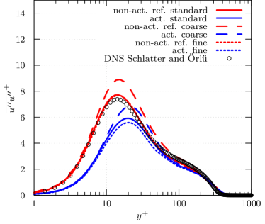
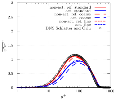
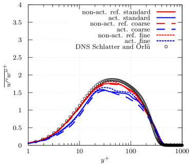
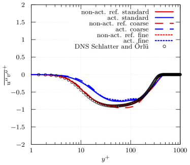
A comparison of the symmetric stresses and the shear-stress component of the Reynolds stress tensor at the streamwise location of , i.e., on the non-actuated surface at , is shown in Fig. 3. The distributions of the standard and the fine mesh nearly collapse for the non-actuated reference case and for the actuated case for all four components. Note that similar results were determined for other actuation parameter configurations. Only on the coarse mesh larger deviations are obtained. Furthermore, the data of the non-actuated reference case for the standard and the fine mesh shows good agreement with DNS data Schlatter2010 of a turbulent boundary layer at a similar Reynolds number, i.e., .
In conclusion, the analysis of the data shows that the resolution of the standard grid can be considered sufficient to accurately predict actuated turbulent boundary layer flow.
| Case | |||||||
|---|---|---|---|---|---|---|---|
| coarse | 20.0 | 1.5 | 8.0 | 78 | |||
| standard | 12.0 | 1.0 | 4.0 | 89 | |||
| fine | 10.0 | 0.7 | 2.0 | 100 |
4.2 Wall-shear stress reductions
The skin-friction reduction is defined in percent by
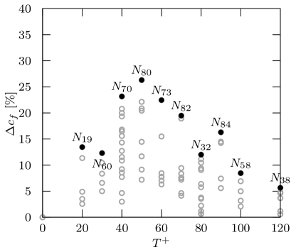
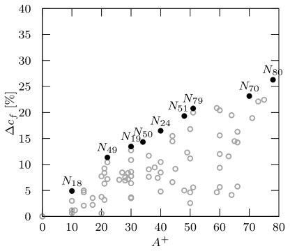
where the wall-shear stress is averaged over the shaded surface in Fig. 2. The values for of the cases are listed in Tab. A1 in the appendix. The dependence of on the various parameters, i.e., the wavelength, period, amplitude, and amplitude velocity, is summarized in Fig. 4. The highlighted and numbered distributions are mainly from cases of the upper envelope of the wall-shear stress reduction, i.e., the maximum values for the wavelength, the period, and the amplitude are emphasized. The discussion and illustration in Fig. 4 summarize the pronounced varying dependence of the wall-shear stress on the different actuation parameters.
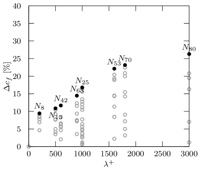

In Fig. LABEL:sub@fig::cfdep::wavelength a quasi-linear increase of the skin-friction reduction as a function of the wavelength is observed. Note, however, that this quasi-linear distribution is achieved by changing simultaneously the amplitude and the period . Especially the latter has to undergo quite a non-linear variation to obtain such an approximately linear growth.
The dependence of on the wave period at various and is presented in Fig. LABEL:sub@fig::cfdep::period. Due to the coupling between the forcing strength and the actuation period, which is in contrast to other actuation methods like spanwise traveling waves of spanwise forcing Du2002 and traveling waves of flexible wall Zhao2004 , the optimum period is determined by an internal, i.e., fluid mechanical, and an external, i.e., actuator, related condition. The ideal is defined by the streak formation time scale Touber2012 , i.e., for oscillatory spanwise forcing the period must be small enough to disrupt the reorganization of the streaks, and a sufficient strength of the forcing, which increases with decreasing period, is required. The dependence of the skin-friction reduction on the period in Fig. LABEL:sub@fig::cfdep::period shows that the optimum period among all cases is on the order of , which is slightly lower than the optimum period of a spanwise oscillating wall in turbulent boundary layer flow Lardeau2013 .
Note that likewise tendencies can be found for spanwise traveling oscillatory forcing Du2002 such as increased drag reduction with higher wavelengths (cf. Fig.LABEL:sub@fig::cfdep::wavelength). The longest wavelength considered in this study () is comparable to that used in the experimental setups by Tamano and Itoh Tamano2012 and Li et al. Li2018 . Although their lowest investigated period is and thus considerably higher than the optimum found in this study, their results corroborate the tendency of higher wall-shear stress reduction at lower periods in the regime .
The distribution of the skin-friction decrease as a function of the amplitude in Fig. LABEL:sub@fig::cfdep::amp shows that the maximum skin-friction reduction is directly coupled to the amplitude. This is to some extent expected since the velocity and thus, the strength of the actuation is directly related to the amplitude. That is, at a given period the strength of the actuation is determined by the amplitude. This is confirmed by the experimental findings of Li et al. Li2018 . They obtain in a lower amplitude range a monotonic increase of the skin-friction reduction for increasing amplitude. Figure LABEL:sub@fig::cfdep::vel presents the skin-friction reductions as a function of the velocity amplitude of the actuation , where the scaling shows a quasi-linear behavior for larger wavelengths .
A similar scaling for was proposed by Tomiyama and Fukagata Tomiyama2013 by combining the amplitude of the actuation velocity (cf. Fig. LABEL:sub@fig::cfdep::vel) and the thickness of the Stokes layer such that which is plotted in Fig. 5. For shorter wavelengths (cf. Fig. LABEL:sub@fig::dr::small), i.e., , a linear scaling is only observed for small values . Note that the current overall reductions are lower than those in Tomiyama2013 which is likely due to the higher Reynolds number in this study ( vs. in Tomiyama2013 ) and due to a generally lower skin-friction reduction efficiency in turbulent boundary layers compared to turbulent channel flow Ricco2004 . For higher scaling factor values, the distribution is more scattered. For larger wavelengths (cf. Fig. LABEL:sub@fig::dr::large), the skin-friction reduction scales almost linearly over the entire range. Above a certain value , however, the linear behavior of the skin-friction reduction deteriorates. We believe the reason for this degradation is the large momentum injection into the boundary layer via too high a velocity amplitude. This increases the spanwise velocity component which leads to an amplified turbulent exchange.


4.3 Drag reduction
Introducing a wave motion of the surface means that the area of the moving wall increases with the amplitude and the wavelength of the wave. The data in Tab. A1 in the appendix shows that this change of the wetted surface can be quite substantial, especially at small wavelengths and high amplitudes. At high wavelengths, this variation becomes rather small. Since the friction drag is defined by the product of the wall-shear stress and the surface interacting with the fluid, the variation of the wetted surface has to be taken into account leading to a non-linear relation between wall-shear stress and friction drag reduction.
The averaged drag reduction is defined as
where is the drag coefficient computed by an integration over the shaded surface in Fig. 2,
The quantity denotes the unit normal vector of the surface, is the unit vector in the -direction, and is the reference surface.
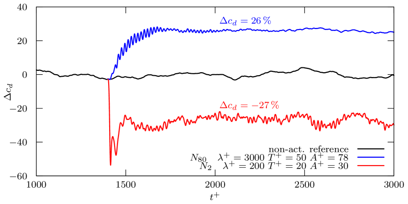
The data in Tab. A1 in the appendix evidences the differences between and , especially at small wavelengths. The highest drag reduction is for a wavelength of , a period of , and an amplitude of . Due to the large wavelength, the increase of the wetted surface is only . The highest drag increase with the highest corresponding skin-friction coefficient increase is observed for , , and . As stated before, this configuration with a small wavelength suffers considerably from a drastic increase of the wetted surface .
The temporal distributions of the instantaneous drag of the ”best” and ”worst”, i.e., highest and lowest drag reduction and , which is a massive drag increase, are compared exemplarily in Fig. 6, with the instantaneous drag of the reference case. The temporal fluctuations of the drag appear stronger for the ”worst” case. Note that due to the larger wavelength the drag of the ”best” case is numerically integrated over a three times larger spanwise extent. Due to the spanwise averaging, this leads to the temporally smoother distribution of the () case compared to the () case.
4.4 Drag reduction modeling and sensitivity analysis
In the following, the drag reduction is modeled as a function of the actuation parameters , , and . For this task, LES simulations provide only a sparse data set comprising 80 points. This amount would roughly correspond to a Cartesian discretization of a three-dimensional data space with only points. However, the modeling is further complicated by the fact that these points are far from regularly distributed. A dense coverage of the actuation space using expensive LES simulations is hardly feasible.
The modeling is performed using a powerful regression solver from machine learning: support vector regression (SVR) Cortes1995 . The algorithm is chosen for its prediction accuracy and its smooth response distribution. SVR is a supervised learning algorithm that constructs a mapping between features or inputs and a known response. Here, SVR maps the actuation parameters , , and on the averaged drag reduction . Note that due to the highly non-linear response behavior and the scarcity of data points at very low wavelengths, cases with wavelengths are ignored during the modeling process. This range is also of little interest as the best drag reduction is found at larger wavelengths. This data exclusion effectively yields 71 data points instead of 80. Overfitting is prevented with a 5-fold cross-validation. The SVR model has a coefficient of determination of indicating an excellent prediction accuracy.
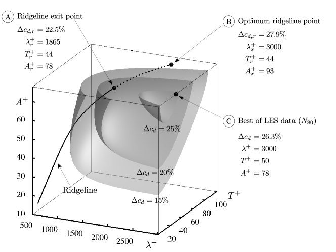
The SVR model from the LES data is employed to visualize a continuous actuation response in the investigated parameter range of , , and . Fig. 7 shows the isosurfaces of three drag reduction levels: , , and %. Within this parameter range, the best performance of 26.5 % is achieved at , and , which is slightly higher than the best simulated LES configuration with %. This location indicates that better drag reduction could be achieved by increasing amplitude and wavelength.
An extrapolation of better performance outside the investigated parameter range is obtained with a ridgeline. In every plane, the drag reduction features a single maximum with respect to the actuation amplitude and period . The curve of connecting all these -dependent maxima is the ridgeline, which is illustrated as a thick black curve in Fig. 7. Variables on this ridgeline are denoted by the subscript ‘r’.
In the range , this maximum is inside the modeled and data range. It is illustrated by the solid black curve. However, the ridgeline leaves this modeled data range through the exit point at the top surface near . The rigdeline is extrapolated outside the data range and depicted as dotted curve between points and . The extrapolation method is detailed in Fernex2019jfm . Along the ridgeline, monotonously increases from 7% at to the maximum of 27.9% at (point ). Note that this point is outside the current LES parameter range.
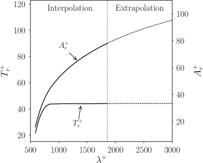
The ridgeline defines a ‘skeleton’ of the parametric behavior as illustrated in Fig. 8. Fig. 8a shows its projection in the and planes. Like in Fig. 7, the dotted sections correspond to the extrapolated ridgeline between points to . The amplitude and period along the ridgeline monotonously increase with the wavelength . The period asymptotes rapidly towards . The amplitude continually increases with the wavelength although at a decreasing rate.
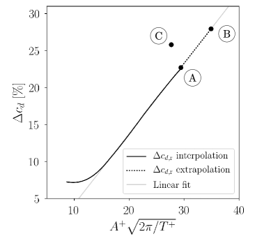
An intriguing physical insight about the drag-reduction mechanism is revealed in Fig. 8b complementing Fig. 5b. The relative drag reduction along the ridgeline is shown as a function of the scaling parameter proposed by Tomiyama and Fukagata Tomiyama2013 based on a Stokes layer of a transverse wall oscillation. clearly exhibits a linear behavior along the ridgeline in the scaling parameter range between 15 and 30. Away from the ridgeline, the scaling shows scatter on the order of that observed in Fig. LABEL:sub@fig::dr::large.

4.5 Turbulent flow statistics
In the following, the mean statistics of a drag reduced flow will be investigated in detail. For this analysis, the case with the highest drag reduction, i.e., the case , will be considered. If data from other cases is used, it is explicitly indicated. All presented wall-normal distributions are considered at the streamwise position , which is located in the actuated region. The actuated fully developed turbulent flow possesses a momentum based Reynolds number . The flow field of the actuated cases is phase averaged in the spanwise direction. Therefore, a triple decomposition Hussain1970 of the flow variables is used
| (3) |
where is the temporal and spanwise average, are periodic fluctuations, are phase averaged quantities, and are stochastic fluctuations. Using this decomposition, represents phase independent quantities, are the periodic fluctuations generated through the actuation, i.e., the secondary flow field, and are turbulent fluctuations. Spanwise averages are obtained along lines of constant distance from the wall, i.e., along the curved mesh lines. This calculation of the spanwise average suffers from some uncertainty for short wavelengths with high amplitudes, where the traveling wave massively intrudes into the boundary layer. For spanwise averages of long wavelengths as in the case, where the local perturbation of the viscous sublayer and the buffer layer is less drastic, this problem does not occur.
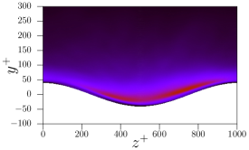
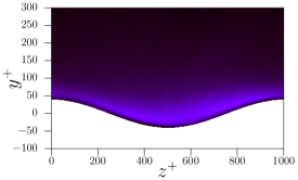
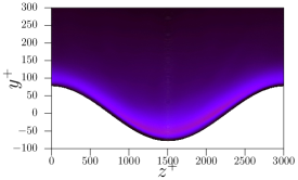
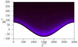
A first overall impression of the impact of the wave actuation on the turbulent coherent structures is given in Fig. 9 by comparing contours of the -criterion Jeong1995 for the random velocity fluctuations . It is evident that the total number of vortical structures in the near-wall region is significantly reduced for the actuated flow. Extended regions of little to hardly any structures occur in Fig. LABEL:sub@fig::lambda2::compare::act. A closer look evidences that unlike the structures of the non-actuated reference flow in Fig. LABEL:sub@fig::lambda2::compare::ref, the structures of the actuated flow are inclined to the left and right depending on the phase angle of the traveling wave. It will be discussed in Sec. 4.6 that this wave determined orientation of the flow structures is an important feature related to drag reduction Touber2012 .
To highlight the influence of the actuation on the instantaneous flow field, Fig. 10 shows contours of the instantaneous random fluctuations of the velocity component in the streamwise direction in a region above the wall. For the non-actuated flow, regions of localized high-speed and low-speed fluid, i.e., streaks, are illustrated whose length and width are on the order of and in inner units. The actuated flow field shows much less pronounced regions of high- and low-speed fluid. That is, the distinctive structure of thin meandering streaks is considerably alleviated compared to the non-actuated reference case.
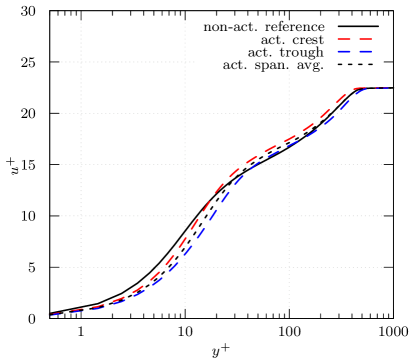
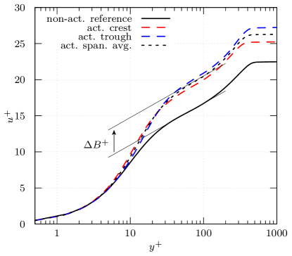
The wall-normal distributions of the phase averaged streamwise velocity above the wave crest and in the wave trough and the mean velocity are shown in Fig. 11. The scaling with the friction velocity of the non-actuated reference case in Fig. LABEL:sub@fig::vel::ref illustrates the decrease of the velocity in the near-wall region. The wall-normal gradient at the wall is lowered, which results in drag reduction. Scaling the velocities with the friction velocity of the actuated wall in Fig. LABEL:sub@fig::vel::nonref leads to an offset of the velocity profiles in the logarithmic region with respect to the non-actuated reference case by . Based on the idea of the analysis of the impact of roughness on fully turbulent flow Nikuradse1933 ; Clauser1956 , Gatti and Quadrio Gatti2016 suggested the offset to predict drag reduction at higher Reynolds numbers
| (4) |
Note, however, that this equation cannot be further simplified since for actuated turbulent boundary layer flow the term is neither constant, as for constant pressure gradient turbulent channel flow, nor can it be substituted by the drag reduction rate, as for constant flow rate turbulent channel flow. Thus, cannot be directly determined by equation (4). Nevertheless, using the local values of , , , and at the calculated offset from equation (4) is , which reasonably agrees with the result shown in Fig. LABEL:sub@fig::vel::nonref. The velocity profiles in Fig. 11 show that for the current actuation neither the non-actuated nor the actuated friction velocity scaling —regardless from crest, trough, or spanwise averaged wall shear scaling— result in a collapsed distribution over the entire boundary layer. In other words, an inner scaling does not hold over the entire boundary layer.
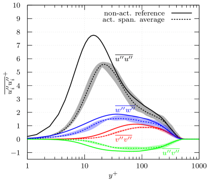
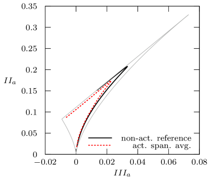
Next, the components of the Reynolds stress tensor are depicted in Fig. 12. Through the actuation, the symmetric Reynolds stresses and the Reynolds shear stress shown in Fig. LABEL:sub@fig::rst::rst are significantly lowered with only minor phase variations. Considering all cases for , a good correlation of the decrease of the skin-friction with the decrease of the peak of the streamwise velocity fluctuations is computed (). For the case , the reductions at , which defines the location of the peak of the streamwise fluctuations and the location of the maximum streamwise velocity streak intensity, are approx. for the streamwise component and for the shear-stress component. This suggests that the turbulent motion close to the wall is massively damped. Touber and Leschziner Touber2012 have reported similarly large reductions in this region for spanwise wall oscillations without normal deflection. They emphasize the importance of the reduced near-wall Reynolds shear stress and drag, as characterized by the Fukagata, Iwamoto, Kasagi (FIK) identity Fukagata2002 , i.e., for the shear-stress contribution . The structural property of the turbulent motion is evidenced by the anisotropy invariant map Lumley1977 in Fig. LABEL:sub@fig::rst::lumley. The stronger suppression of the streamwise fluctuations compared to the other components is illustrated by the shift of the actuated distribution away from one-dimensional turbulence in the upper right vertex to isotropic turbulence in the lower vertex.
The distributions of the joint probability density function (PDF) of the streamwise and the wall-normal stochastic velocity fluctuations and are presented in Fig. 13. High values in the upper left quadrant (negative and positive ) denote ejections of fluid from the near-wall region towards the outer flow, whereas high values in the lower right quadrant (positive and negative ) indicate sweeps of high-speed fluid from the outer flow towards the near-wall region. As can be seen in Fig. 13, an overall attenuation of the fluctuations is observed with a strong damping of the sweeps and ejections in the second and the fourth quadrant. Again, this is in agreement with the results from spanwise oscillating walls without normal deflection Agostini2014 ; Touber2012 .

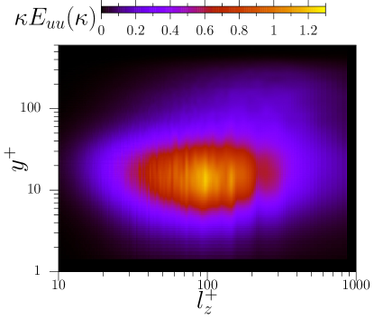
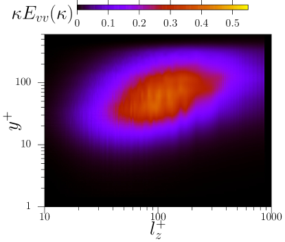
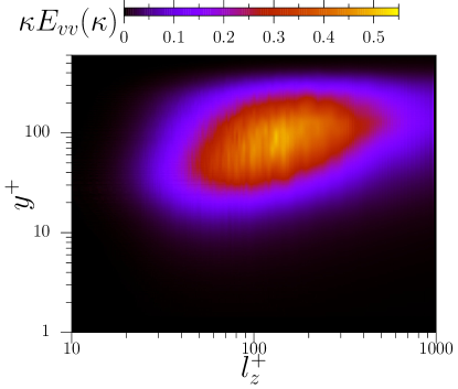
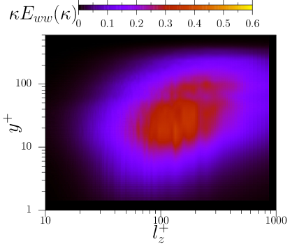
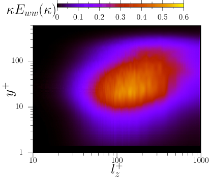
Spanwise premultiplied energy spectra of the velocity fluctuations , where is the wavenumber, are presented in Fig. 14. Each spectrum is normalized by the total resolved energy of the corresponding velocity component and the related case, i.e., the non-actuated reference case and . No general decrease in the energy peak of the actuated case is observed, only a shift in the energy distribution as a function of the structural wavelength and wall-normal coordinate can be seen. A comparison between the two differently normalized spectra for the streamwise component (cf. Fig. LABEL:sub@fig::spectra::u::ref and Fig. LABEL:sub@fig::spectra::u::act) shows an energy decrease especially for the small scales and in the near-wall region. In other words, for the actuated case the energy is accumulated further off the wall in the larger scale turbulent structures. The peak of the non-actuated reference case at , which is associated with the typical spacing of the near-wall streaks of , becomes less pronounced for the actuated case and is shifted off the wall. This observation corroborates the visual impression from Fig. 10 of a strong reduction of the near-wall streaks for the actuated case. Similar tendencies are observed for the wall-normal (cf. Fig. LABEL:sub@fig::spectra::v::ref and Fig. LABEL:sub@fig::spectra::v::act) and the spanwise velocity component (cf. Fig. LABEL:sub@fig::spectra::w::ref and Fig. LABEL:sub@fig::spectra::w::act). Additionally, a stronger concentration of the energy in the length scale range of the near-wall streaks is observed for the spanwise velocity component. There is a sharper peak for the actuated case in comparison to a broader energy distribution in the non-actuated case.

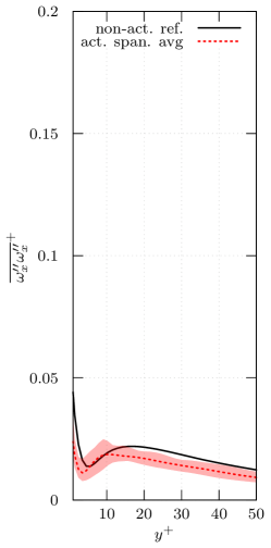
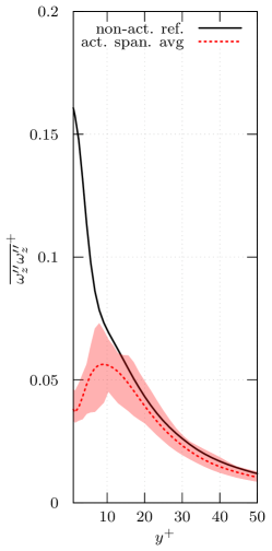
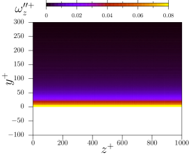
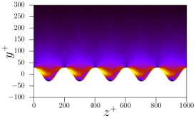
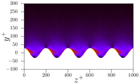
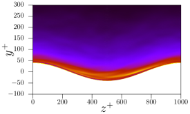
In Fig. 15 the phase averaged and spanwise averaged distributions of the vorticity fluctuations are presented as a function of the wall-normal distance. The comparison of the profiles of each component shows that the major attenuation is observed in the wall-normal and the spanwise components, whereas the streamwise component shows only minor changes. Generally, for all cases with a good correlation between the decrease of the skin-friction and the decrease of the peak of the wall-normal () and spanwise () vorticity fluctuations was found. Again, similar vorticity trends were reported for spanwise oscillating walls Touber2012 . The drag reduction was discussed to be caused by the weakening of velocity streaks near Agostini2014 . That is, at least for actuation with large wavelengths , a direct interference with quasi-streamwise vortices Tomiyama2013 has a minor effect on drag reductions.
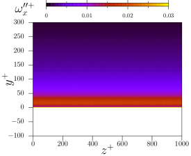
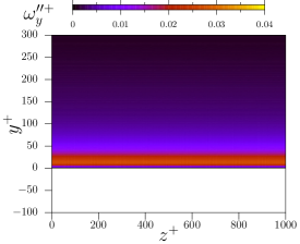
The comparison of the vorticity fluctuation contours for four cases, i.e., the non-actuated reference case, the case with the highest drag increase , a case with moderate drag reduction , and the case with the highest drag reduction , in Fig. 16 shows details about the phase dependence of the overall structure of the vorticity field. It is obvious that the drag increase is associated with strongly enlarged and highly phase dependent vorticity contours. Due to the high amplitude and short wavelength sinusoidal wall motion, the boundary layer flow is massively perturbed. This is completely different for the two drag reduction cases, where the overall boundary layer structure is maintained but with reduced values of the wall-normal and spanwise vorticity component. Phase variations occur especially for the wall-normal component with the highest decrease above the wave crest and the lowest decrease in the wave trough. Note, however, that despite the clear phase variations, the overall lowered vorticity levels are maintained throughout the entire actuation period, as shown in Fig. 15.


4.6 Spanwise shear
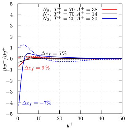
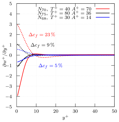
To investigate the secondary flow strength and its effect on the near-wall turbulent structures, the Stokes strain , i.e., the rate of change in the wall-normal direction of the periodic fluctuations of the spanwise velocity component, is considered in Fig. 17 for cases with wavelengths , , , and . Based on the data summarized in Tab A1 in the appendix, for each set the cases with the highest, medium, and lowest skin-friction reduction are shown. The Stokes strain is used to characterize the Stokes layer that develops above an oscillating wall without any wall-normal deflection. However, similar to a configuration with pure spanwise oscillating walls Jung1992 ; Touber2012 a Stokes-like layer is also generated by a transversal wave motion of the surface. Through the introduction of a periodic wall-normal velocity , a periodic spanwise velocity component is induced via mass conservation resulting in a wall-normal shear distribution defining a Stokes layer. Cases with a high drag reduction generally show a high level of symmetric, i.e., positive and negative, spanwise shear very close to the wall, whereas less symmetric shear distributions yield lower drag reduction. When the Stokes drag significantly increases near the wall, i.e., a singular-like distribution occurs, the drag reduction reduces drastically. This observation supports the assumption that the drag reduction mechanism is strongly linked to spanwise oscillations which are generated either by wave oscillations Touber2012 , traveling waves of spanwise forcing Du2002 , spanwise velocity at the wall Zhao2004 , or spanwise transversal surface waves Klumpp2010b ; Koh2015 .
The assumption of the importance of the oscillating spanwise shear for skin-friction reduction also yields an explanation for the increasing skin-friction reduction with growing wavelength, which agrees with an observation of Du et al. Du2002 . For short wavelengths, e.g., , the integration of the spanwise shear distribution over the spanwise width of a near-wall streak, i.e., , results in only a minor force in the spanwise direction acting on the streaks. For wavelengths , however, the spanwise shear varies only slightly over the width of a streak, therefore a considerable spanwise force is determined by the integration over the spanwise streak width. Note that this behavior does not occur for spanwise wall oscillations, since the periodic spanwise shear does not depend on the spanwise coordinate.


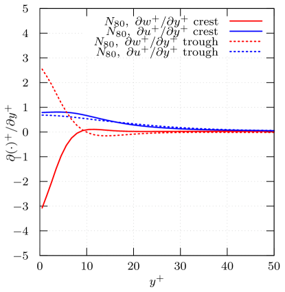
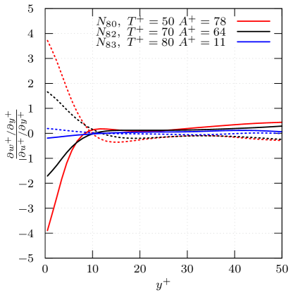
A comparison of spanwise and streamwise shear is shown in Fig. 18. Touber and Leschziner Touber2012 discuss a certain optimal scenario for oscillatory forcing in turbulent channel flow, where the ratio of spanwise to streamwise shear reaches values of up to . Fig. LABEL:sub@fig::shearuw::ratio shows that a similar value of this ratio is obtained for the case with the highest skin-friction reduction , whereas a lower ratio is obtained for the cases with medium () and low () skin-friction reduction. For all cases, the change of the skin-friction is well correlated, i.e., at the wave crest and in the wave trough, with a spanwise-to-streamwise shear ratio of .
Overall, the results for the spanwise traveling transversal waves in Fig. 17 underline the similarities to other drag reduction techniques based on periodic spanwise forcing. The results of the cases with lower wavelength in combination with high amplitude and high frequency deviate from this observation due to the increased wetted surface.
4.7 Energy saving analysis
The previous discussion has shown that considerable drag reduction rates have been obtained. However, drag reduction is not the only metric of interest. From a prospective application point of view, the question of net energy saving and its relation to drag reduction must be addressed. The ideal net energy saving is defined as
| (5) |
where is the power necessary to overcome the friction and pressure forces of the non-actuated and actuated surface in the streamwise direction. The power spent on control , i.e., on deflecting the surface for the traveling wave, is computed by
| (6) |
where is a combination of the unit vectors in the streamwise and wall-normal direction. Hence, is a combination of the viscous and pressure forces effective in the -direction multiplied by the speed of the wall motion in the -direction. The values of and are depicted in Fig. 19 for all cases. The data for are also listed in Tab. A1 in the appendix. Fig. LABEL:sub@fig::power::control shows the expected approximately linear dependence between the power spent and the actuation velocity cubed .
It is evident from Fig. LABEL:sub@fig::power::net that net power saving is only obtained for a few cases with a maximum of for case . Most cases clearly show no net power saving but net power loss. For instance, for is , i.e., almost the fourfold has to be invested.
A closer look at the net-power-saving cases in Fig. LABEL:sub@fig::power::netdetail shows that high drag reduction rates are no indicator for high net power saving. That is, there is no linear relation between drag reduction and net power saving. Instead, a high value of the scaling parameter obtained by a low amplitude speed leads to positive net power saving. Thus, as expected, there is a trade-off between the minimum power input to effectively influence the turbulent boundary layer and a maximum power input above which the energy costs grow tremendously. In the current parameter range, the optimum energy saving solution, i.e., , is achieved for the case with , , and , which possesses just a medium drag reduction of . Note that the parameters that result in high net energy saving are in the upper range of the interval. Furthermore, the data in Tab. A1 in the appendix indicates that the sensitivity of is less pronounced for larger wavelength and above a wave period of .


5 Conclusions
To analyze drag reducing effects and the net energy saving potential of spanwise traveling transversal surface waves high-resolution large-eddy simulations were conducted. The parameter space defined by the wave amplitude, wave period, and wavelength was investigated based on wave parameter setups for purely spanwise traveling waves. The variation of skin-friction reduction, i.e., mean wall-shear stress alteration, drag reduction, i.e., surface integrated wall-shear stress, and net energy saving was analyzed. In brief, a maximum drag reduction and net energy saving of and was found.
The highest skin-friction reduction was achieved for a period of , which is lower than the one reported for spanwise oscillating wall and within the range of the streak formation time scale. Larger wavelengths and amplitudes yielded higher skin-friction reduction. For wavelengths larger than 1000 plus units, a scaling with the Stokes layer height and the velocity amplitude was found to predict skin-friction reduction reasonably well. Additionally, the difference between skin-friction reduction and drag reduction, i.e., the increase of the wetted surface was taken into account, was found to be substantial for short wavelengths in combination with high amplitudes. A drag-reduction model was derived from the sparse dataset using optimized support vector regression. From the model, a tendency to an asymptotic behavior of amplitude and period could be identified, supporting the assumption of an optimum period in the range for large wavelengths. Moreover, a ridgeline behavior of optimum drag reduction in the high wavelength regime was extracted from the model.
The statistical results of the turbulent flow field confirmed this result for high wavelength configurations, where similar effects of the actuation on the near-wall region compared to spanwise oscillating walls were observed. That is, considerable reductions of the near-wall velocity streak strength were found for the cases with high drag reduction. For the highest drag reduction case, the smaller wall-shear stress was coupled to a substantial decrease of the Reynolds shear stress in the near-wall region. Generally, for large wavelength cases the decrease of the wall-normal and spanwise vorticity fluctuations strongly correlated with skin-friction reduction and drag reduction. A comparison among several configurations revealed that for unfavorable combinations of short wavelength and high amplitude, a considerable increase of the turbulent exchange resulting in skin-friction and drag increase was observed, whereas large wavelengths circumvented this effect and led to drag reduction. The periodic secondary flow field generated by the wavy surface motion approximated that of Stokes flow. Similar oscillating spanwise shear distributions were observed for many drag reducing cases, although no perfectly symmetrical oscillatory excitation of the near-wall structures is achieved.
No linear relationship between drag reduction and net energy saving was determined. That is, due to the non-linear response of the near-wall flow to the actuation the highest drag reduction does not result in the highest net energy saving. The maximum net energy saving was achieved for a drag reduction of , which is clearly lower than the maximum drag reduction of . A high value of the product of the actuation amplitude speed and the thickness of the Stokes layer at low amplitude speed results in positive net energy saving. The susceptibility of is less pronounced for larger wavelength, which is a promising observation for prospective applications.
Acknowledgements
The research was funded by the Deutsche Forschungsgemeinschaft (DFG) in the framework of the research projects SCHR 309/52 and SCHR 309/68. The authors gratefully acknowledge the Gauss Centre for Supercomputing e.V. (www.gauss-centre.eu) for funding this project by providing computing time on the GCS Supercomputers Hazelhen at HLRS Stuttgart and JURECA at Jülich Supercomputing Centre (JSC). BRN acknowledges support from the French National Research Agency (ANR) under grant ANR-17-ASTR-0022 (FlowCon).
Compliance with Ethical Standards
Conflict of Interests
The authors declare that they have no conflicts of interest.
Appendix A Appendix
| 1 | 1000 | 0 | 0 | 0 | 0 | 0 | 0.0 | 0 |
| 2 | 1000 | 200 | 20 | 30 | -27 | -7 | 19.4 | -100 |
| 3 | 1000 | 200 | 30 | 21 | -1 | 8 | 10.1 | -17 |
| 4 | 1000 | 200 | 40 | 30 | -9 | 9 | 19.4 | -24 |
| 5 | 1000 | 200 | 50 | 45 | -26 | 9 | 39.0 | -42 |
| 6 | 1000 | 200 | 60 | 30 | -10 | 8 | 19.4 | -17 |
| 7 | 1000 | 200 | 70 | 14 | 0 | 5 | 4.7 | -1 |
| 8 | 1000 | 200 | 70 | 38 | -17 | 9 | 29.4 | -24 |
| 9 | 1000 | 200 | 100 | 28 | -9 | 7 | 17.2 | -11 |
| 10 | 1000 | 500 | 20 | 30 | 0 | 4 | 3.5 | -98 |
| 11 | 1000 | 500 | 30 | 22 | 9 | 10 | 1.9 | -10 |
| 12 | 1000 | 500 | 40 | 21 | 8 | 9 | 1.7 | -1 |
| 13 | 1000 | 500 | 40 | 30 | 8 | 11 | 3.5 | -10 |
| 14 | 1000 | 500 | 60 | 30 | 5 | 8 | 3.5 | -2 |
| 15 | 1000 | 500 | 70 | 36 | 3 | 8 | 4.9 | -4 |
| 16 | 1000 | 500 | 70 | 64 | -10 | 4 | 14.6 | -33 |
| 17 | 1000 | 500 | 100 | 48 | -3 | 5 | 8.6 | -10 |
| 18 | 1000 | 1000 | 20 | 10 | 5 | 5 | 0.1 | -6 |
| 19 | 1000 | 1000 | 20 | 30 | 13 | 13 | 0.9 | -88 |
| 20 | 1000 | 1000 | 20 | 50 | 0 | 3 | 2.4 | -289 |
| 21 | 1000 | 1000 | 40 | 10 | 3 | 3 | 0.1 | 1 |
| 22 | 1000 | 1000 | 40 | 20 | 7 | 8 | 0.4 | 0 |
| 23 | 1000 | 1000 | 40 | 30 | 12 | 13 | 0.9 | -4 |
| 24 | 1000 | 1000 | 40 | 40 | 15 | 16 | 1.6 | -14 |
| 25 | 1000 | 1000 | 40 | 50 | 15 | 17 | 2.4 | -32 |
| 26 | 1000 | 1000 | 40 | 60 | 13 | 16 | 3.5 | -55 |
| 27 | 1000 | 1000 | 80 | 10 | 1 | 1 | 0.1 | 0 |
| 28 | 1000 | 1000 | 80 | 20 | 3 | 4 | 0.4 | 2 |
| 29 | 1000 | 1000 | 80 | 30 | 6 | 6 | 0.9 | 3 |
| 30 | 1000 | 1000 | 80 | 40 | 9 | 10 | 1.6 | 4 |
| 31 | 1000 | 1000 | 80 | 50 | 9 | 11 | 2.4 | 1 |
| 32 | 1000 | 1000 | 80 | 60 | 9 | 12 | 3.5 | -3 |
| 33 | 1000 | 1000 | 120 | 10 | 1 | 1 | 0.1 | 1 |
| 34 | 1000 | 1000 | 120 | 20 | 0 | 1 | 0.4 | 0 |
| 35 | 1000 | 1000 | 120 | 30 | 3 | 4 | 0.9 | 2 |
| 36 | 1000 | 1000 | 120 | 40 | 3 | 5 | 1.6 | 1 |
| 37 | 1000 | 1000 | 120 | 50 | 2 | 5 | 2.4 | -1 |
| 38 | 1000 | 1000 | 120 | 60 | 2 | 6 | 3.5 | -3 |
| 39 | 1200 | 0 | 0 | 0 | 0 | 0 | 0.0 | 0 |
| 40 | 1200 | 600 | 30 | 44 | 2 | 7 | 5.1 | -74 |
| 41 | 1200 | 600 | 40 | 59 | -4 | 5 | 8.9 | -71 |
| 42 | 1200 | 600 | 50 | 36 | 9 | 12 | 3.5 | -6 |
| 43 | 1200 | 600 | 60 | 21 | 5 | 6 | 1.2 | 2 |
| 44 | 1200 | 600 | 70 | 29 | 6 | 8 | 2.3 | 2 |
| 45 | 1200 | 600 | 80 | 66 | -5 | 6 | 11.0 | -23 |
| 46 | 1200 | 600 | 90 | 51 | -1 | 6 | 6.8 | -10 |
| 47 | 1200 | 600 | 100 | 14 | 2 | 2 | 0.5 | 1 |
| 48 | 1600 | 0 | 0 | 0 | 0 | 0 | 0.0 | 0 |
| 49 | 1600 | 1600 | 20 | 22 | 11 | 11 | 0.2 | -47 |
| 50 | 1600 | 1600 | 40 | 34 | 14 | 14 | 0.4 | -6 |
| 51 | 1600 | 1600 | 40 | 48 | 19 | 19 | 0.9 | -23 |
| 52 | 1600 | 1600 | 50 | 60 | 19 | 20 | 1.4 | -17 |
| 53 | 1600 | 1600 | 50 | 73 | 21 | 22 | 2.0 | -35 |
| 54 | 1600 | 1600 | 60 | 27 | 8 | 8 | 0.3 | 4 |
| 55 | 1600 | 1600 | 70 | 71 | 17 | 19 | 1.9 | -4 |
| 56 | 1600 | 1600 | 80 | 17 | 2 | 2 | 0.1 | 1 |
| 57 | 1600 | 1600 | 90 | 65 | 13 | 14 | 1.6 | 4 |
| 58 | 1600 | 1600 | 100 | 40 | 8 | 8 | 0.6 | 5 |
| 59 | 1800 | 0 | 0 | 0 | 0 | 0 | 0.0 | 0 |
| 60 | 1800 | 900 | 30 | 49 | 10 | 12 | 2.9 | -84 |
| 61 | 1800 | 900 | 40 | 63 | 7 | 12 | 4.7 | -69 |
| 62 | 1800 | 900 | 50 | 22 | 7 | 7 | 0.6 | 2 |
| 63 | 1800 | 900 | 50 | 44 | 12 | 14 | 2.3 | -8 |
| 64 | 1800 | 900 | 70 | 28 | 7 | 8 | 0.9 | 3 |
| 65 | 1800 | 900 | 80 | 17 | 3 | 4 | 0.4 | 2 |
| 66 | 1800 | 900 | 80 | 60 | 6 | 9 | 4.3 | -8 |
| 67 | 1800 | 900 | 90 | 39 | 6 | 7 | 1.8 | 2 |
| 68 | 1800 | 1800 | 30 | 14 | 5 | 5 | 0.1 | -2 |
| 69 | 1800 | 1800 | 40 | 51 | 19 | 20 | 0.8 | -27 |
| 70 | 1800 | 1800 | 40 | 70 | 22 | 23 | 1.5 | -67 |
| 71 | 1800 | 1800 | 50 | 59 | 20 | 21 | 1.1 | -15 |
| 72 | 1800 | 1800 | 60 | 44 | 15 | 15 | 0.6 | 3 |
| 73 | 1800 | 1800 | 60 | 75 | 21 | 22 | 1.7 | -14 |
| 74 | 1800 | 1800 | 70 | 29 | 7 | 7 | 0.3 | 4 |
| 75 | 1800 | 1800 | 80 | 36 | 9 | 9 | 0.4 | 5 |
| 76 | 1800 | 1800 | 90 | 66 | 13 | 14 | 1.3 | 4 |
| 77 | 1800 | 1800 | 100 | 21 | 3 | 3 | 0.1 | 2 |
| 78 | 3000 | 0 | 0 | 0 | 0 | 0 | 0.0 | 0 |
| 79 | 3000 | 3000 | 40 | 51 | 21 | 21 | 0.3 | -17 |
| 80 | 3000 | 3000 | 50 | 78 | 26 | 26 | 0.7 | -20 |
| 81 | 3000 | 3000 | 60 | 26 | 7 | 7 | 0.1 | 4 |
| 82 | 3000 | 3000 | 70 | 64 | 19 | 19 | 0.4 | 8 |
| 83 | 3000 | 3000 | 80 | 11 | 1 | 1 | 0.0 | 1 |
| 84 | 3000 | 3000 | 90 | 66 | 16 | 16 | 0.5 | 10 |
References
- (1) Agostini, L., Touber, E., Leschziner, M.A.: Spanwise oscillatory wall motion in channel flow: drag-reduction mechanisms inferred from DNS-predicted phase-wise property variations at . J. Fluid Mech. 743, 606–635 (2014)
- (2) Albers, M., Meysonnat, P.S., Schröder, W.: Actively reduced airfoil drag by transversal surface waves. Flow Turbul. Combust. 102(4), 865–886 (2019)
- (3) Alkishriwi, N., Meinke, M., Schröder, W.: A large-eddy simulation method for low Mach number flows using preconditioning and multigrid. Comp. Fluids 35(10), 1126–1136 (2006)
- (4) Bechert, D.W., Hoppe, G., Reif, W.E.: On the drag reduction of the shark skin. AIAA Paper No. 85-0546 (1985)
- (5) Boris, J.P., Grinstein, F.F., Oran, E.S., Kolbe, R.L.: New insights into large eddy simulation. Fluid Dyn. Res. 10(4-6), 199–228 (1992)
- (6) Choi, K.S., Debisschop, J.R., Clayton, B.R.: Turbulent boundary-layer control by means of spanwise-wall oscillation. AIAA Journal 36(7), 1157–1163 (1998)
- (7) Choi, K.S., Yang, X., Clayton, B.R., Glover, E.J., Atlar, M., Semenov, B.N., Kulik, V.M.: Turbulent drag reduction using compliant surfaces. Proc. R. Soc. London, Ser. A 453(1965), 2229–2240 (1997)
- (8) Clauser, F.H.: The turbulent boundary layer. pp. 1–51. Elsevier (1956)
- (9) Cortes, C., Vapnik, V.: Support-vector networks. Machine learning 20(3), 273–297 (1995)
- (10) Du, Y., Karniadakis, G.E.: Suppressing wall turbulence by means of a transverse traveling wave. Science 288(5469), 1230–1234 (2000)
- (11) Du, Y., Symeonidis, V., Karniadakis, G.E.: Drag reduction in wall-bounded turbulence via a transverse travelling wave. J. Fluid Mech. 457, 1–34 (2002)
- (12) Fernex, D., Semann, R., Albers, M., Meysonnat, P.S., Schröder, W., Noack, B.R.: Self-similar drag reduction formula from sparse data—optimization of turbulent skin-friction via spanwise travelling surface waves. J. Fluid Mech. In preparation. The preprint will be made available in arXiv. (2019)
- (13) Fukagata, K., Iwamoto, K., Kasagi, N.: Contribution of Reynolds stress distribution to the skin friction in wall-bounded flows. Phys. Fluids 14(11), L73–L76 (2002)
- (14) García-Mayoral, R., Jiménez, J.: Drag reduction by riblets. Philos. Trans. R. Soc. London, Ser. A 369(1940), 1412–1427 (2011)
- (15) García-Mayoral, R., Jiménez, J.: Hydrodynamic stability and breakdown of the viscous regime over riblets. J. Fluid Mech. 678, 317–347 (2011)
- (16) Gatti, D., Quadrio, M.: Reynolds-number dependence of turbulent skin-friction drag reduction induced by spanwise forcing. J. Fluid Mech. 802, 553–582 (2016)
- (17) Hirt, C.W., Amsden, A.A., Cook, J.L.: An arbitrary Lagrangian–Eulerian computing method for all flow speeds. J. Comput. Phys. 14, 227–253 (1974)
- (18) Hussain, A.K.M.F., Reynolds, W.C.: The mechanics of an organized wave in turbulent shear flow. J. Fluid Mech. 41(2), 241–258 (1970)
- (19) Ishar, R., Kaiser, E., Morzyński, M., Fernex, D., Semaan, R., Albers, M., Meysonnat, P.S., Schröder, W., Noack, B.R.: Metric for attractor overlap. J. Fluid Mech. 874, 720–755 (2019)
- (20) Itoh, M., Tamano, S., Yokota, K., Taniguchi, S.: Drag reduction in a turbulent boundary layer on a flexible sheet undergoing a spanwise traveling wave motion. J. Turbul. 7, N27 (2006)
- (21) Jeong, J., Hussain, F.: On the identification of a vortex. J. Fluid Mech. 285, 69–94 (1995)
- (22) Jung, W.J., Mangiavacchi, N., Akhavan, R.: Suppression of turbulence in wall‐bounded flows by high‐frequency spanwise oscillations. Phys. Fluids A 4(8), 1605–1607 (1992)
- (23) Kim, E., Choi, H.: Space-time characteristics of a compliant wall in a turbulent channel flow. J. Fluid Mech. 756, 30–53 (2014)
- (24) Klumpp, S., Meinke, M., Schröder, W.: Numerical simulation of riblet controlled spatial transition in a zero-pressure-gradient boundary layer. Flow Turbul. Combust. 85(1), 57–71 (2010a)
- (25) Klumpp, S., Meinke, M., Schröder, W.: Drag reduction by spanwise transversal surface waves. J. Turbul. 11 (2010b)
- (26) Klumpp, S., Meinke, M., Schröder, W.: Friction drag variation via spanwise transversal surface waves. Flow Turbul. Combust. 87(1), 33–53 (2011)
- (27) Koh, S.R., Meysonnat, P., Meinke, M., Schröder, W.: Drag reduction via spanwise transversal surface waves at high Reynolds numbers. Flow Turbul. Combust. 95(1), 169–190 (2015)
- (28) Koh, S.R., Meysonnat, P., Statnikov, V., Meinke, M., Schröder, W.: Dependence of turbulent wall-shear stress on the amplitude of spanwise transversal surface waves. Comput. Fluids 119, 261–275 (2015)
- (29) Lardeau, S., Leschziner, M.A.: The streamwise drag-reduction response of a boundary layer subjected to a sudden imposition of transverse oscillatory wall motion. Phys. Fluids 25(7), 075109 (2013)
- (30) Li, W., Roggenkamp, D., Hecken, T., Jessen, W., Klaas, M., Schröder, W.: Parametric investigation of friction drag reduction in turbulent flow over a flexible wall undergoing spanwise transversal traveling waves. Exp. Fluids 59(6), 105 (2018)
- (31) Luhar, M., Sharma, A., McKeon, B.: A framework for studying the effect of compliant surfaces on wall turbulence. J. Fluid Mech. 768, 415–441 (2015)
- (32) Lumley, J.L., Newman, G.R.: The return to isotropy of homogeneous turbulence. J. Fluid Mech. 82(01), 161–178 (1977)
- (33) Meinke, M., Schröder, W., Krause, E., Rister, T.: A comparison of second- and sixth-order methods for large-eddy simulations. Comput. Fluids 31(4), 695–718 (2002)
- (34) Meysonnat, P.S., Roggenkamp, D., Li, W., Roidl, B., Schröder, W.: Experimental and numerical investigation of transversal traveling surface waves for drag reduction. Eur. J. Mech. B. Fluids 55, 313–323 (2016)
- (35) Moin, P., Shih, T., Driver, D., Mansour, N.N.: Direct numerical simulation of a three‐dimensional turbulent boundary layer. Phys. Fluids A 2(10), 1846–1853 (1990)
- (36) Nikuradse, J.: Strömungsgesetze in rauhen Rohren. VDI-Forschungsheft 361 (1933)
- (37) Quadrio, M.: Drag reduction in turbulent boundary layers by in-plane wall motion. Philos. Trans. R. Soc. London, Ser. A 369(1940), 1428–1442 (2011)
- (38) Quadrio, M., Ricco, P.: Critical assessment of turbulent drag reduction through spanwise wall oscillations. J. Fluid Mech. 521, 251–271 (2004)
- (39) Renze, P., Schröder, W., Meinke, M.: Large-eddy simulation of film cooling flows at density gradients. Int. J. Heat Fluid Flow 29(1), 18–34 (2008)
- (40) Ricco, P.: Modification of near-wall turbulence due to spanwise wall oscillations. J. Turbul. 5, N24 (2004)
- (41) Ricco, P., Wu, S.: On the effects of lateral wall oscillations on a turbulent boundary layer. Exp. Therm Fluid Sci. 29(1), 41–52 (2004)
- (42) Roidl, B., Meinke, M., Schröder, W.: A reformulated synthetic turbulence generation method for a zonal RANS–LES method and its application to zero-pressure gradient boundary layers. Int. J. Heat Fluid Flow 44, 28–40 (2013)
- (43) Rütten, F., Schröder, W., Meinke, M.: Large-eddy simulation of low frequency oscillations of the Dean vortices in turbulent pipe bend flows. Phys. Fluids 17(3), 035107 (2005)
- (44) Schlatter, P., Örlü, R.: Assessment of direct numerical simulation data of turbulent boundary layers. J. Fluid Mech. 659, 116–126 (2010)
- (45) Spalart, P.R., McLean, J.D.: Drag reduction: enticing turbulence, and then an industry. Philos. Trans. R. Soc. London, Ser. A 369(1940), 1556–1569 (2011)
- (46) Statnikov, V., Meinke, M., Schröder, W.: Reduced-order analysis of buffet flow of space launchers. J. Fluid Mech. 815, 1–25 (2017)
- (47) Tamano, S., Itoh, M.: Drag reduction in turbulent boundary layers by spanwise traveling waves with wall deformation. J. Turbul. 13, N9 (2012)
- (48) Tomiyama, N., Fukagata, K.: Direct numerical simulation of drag reduction in a turbulent channel flow using spanwise traveling wave-like wall deformation. Phys. Fluids 25(10), 105115 (2013)
- (49) Touber, E., Leschziner, M.A.: Near-wall streak modification by spanwise oscillatory wall motion and drag-reduction mechanisms. J. Fluid Mech. 693, 150–200 (2012)
- (50) Walsh, M., Weinstein, L.: Drag and heat transfer on surfaces with small longitudinal fins. In: 11th Fluid and Plasma Dynamics Conference, p. 1161 (1978)
- (51) Walsh, M.J., Sellers III, W.L., Mcginley, C.B.: Riblet drag at flight conditions. J. Aircraft 26(6), 570–575 (1989)
- (52) Yudhistira, I., Skote, M.: Direct numerical simulation of a turbulent boundary layer over an oscillating wall. J. Turbul. 12, N9 (2011)
- (53) Zhang, C., Wang, J., Blake, W., Katz, J.: Deformation of a compliant wall in a turbulent channel flow. J. Fluid Mech. 823, 345–390 (2017)
- (54) Zhao, H., Wu, J.Z., Luo, J.S.: Turbulent drag reduction by traveling wave of flexible wall. Fluid Dyn. Res. 34(3), 175–198 (2004)