Data-driven retrieval of primary plane-wave responses

Department of Geoscience and Engineering, Delft University of Technology, Stevinweg 1, 2628 CN Delft, The Netherlands
G.A.Meles@tudelft.nl
Keywords: Seismic imaging, Multiple attenuation, Reverse-time migration

1 Abstract

Seismic images provided by reverse time migration can be contaminated by artefacts associated with the migration of multiples. Multiples can corrupt seismic images, producing both false positives, i.e. by focusing energy at unphysical interfaces, and false negatives, i.e. by destructively interfering with primaries. Multiple prediction / primary synthesis methods are usually designed to operate on point source gathers, and can therefore be computationally demanding when large problems are considered. A computationally attractive scheme that operates on plane-wave datasets is derived by adapting a data-driven point source gathers method, based on convolutions and cross-correlations of the reflection response with itself, to include plane-wave concepts. As a result, the presented algorithm allows fully data-driven synthesis of primary reflections associated with plane-wave source responses. Once primary plane-wave responses are estimated, they are used for multiple-free imaging via plane-wave reverse time migration. Numerical tests of increasing complexity demonstrate the potential of the proposed algorithm to produce multiple-free images from only a small number of plane-wave datasets.

2 Introduction

Most standard processing steps, e.g. velocity analysis (Yilmaz, (2001)) and reverse time migration (Whitmore, (1983); McMechan, (1983); Zhu et al., (1998); Gray et al., (2001); Mulder and Plessix, (2004)), are based on linear (Born) approximations, for which multiply scattered waves represent a source of coherent noise. When linearized methods are employed, multiples should then be suppressed to avoid concomitant artefacts. Free-surface multiples particularly affect seismic images resulting from marine data (Wiggins, (1988)), and many algorithms have been designed to attenuate the presence of free-surface multiples (for a comprehensive review see Dragoset et al., (2010)). On the other hand, internal multiples strongly contaminate both land (Kelamis et al., (2006)) and marine data (van Borselen, (2002)). Fewer techniques have been designed to estimate and remove internal multiples. The seminal method by Jakubowicz, (1998) uses combinations of three observed reflections to predict and remove internal multiples. However, this scheme requires prior information about reflections to allow proper multiple prediction and removal. On the other hand, applications of inverse scattering methods (Weglein et al., (1997)) can predict all orders of internal multiple reflections with approximate amplitudes in one step without model information (ten Kroode, (2002); Löer et al., (2016); Zhang et al., 2019a ).

Multiple-related artefacts can also be dealt with via Marchenko methods. Marchenko redatuming estimates Green’s functions between arbitrary locations inside a medium and real receivers located at the surface (Broggini et al., (2012); Wapenaar et al., (2012, 2014); da Costa Filho et al., (2014)). In Marchenko redatuming, Green’s functions are estimated using reciprocity theorems involving so called ‘focusing functions’, i.e. wavefields which achieve focusing properties in the subsurface (Slob et al., (2014)). In contrast to seismic interferometry, Marchenko redatuming requires an estimate of the direct wave from the virtual sources to the surface receivers, only one sided illumination of the medium and no physical receivers at the position of the virtual sources (Broggini et al., (2012); Wapenaar et al., (2014)). Focusing functions and redatumed Green’s functions can provide multiple-free images directly (Slob et al., (2014); Wapenaar et al., (2014)). Moreover, combining Marchenko methods and convolutional interferometry allows estimating internal multiples in the data at the surface (Meles et al., (2015); da Costa Filho et al., 2017b ). Other applications of the Marchenko method include microseismic source localization (Behura and Snieder, (2013); van der Neut et al., (2017); Brackenhoff et al., (2019)), inversion (Slob and Wapenaar, (2014); van der Neut and Fokkema, (2018)), homogeneous Green’s functions retrieval (Reinicke and Wapenaar, (2019); Wapenaar et al., (2018)) and various wavefield focusing techniques (Meles et al., (2019)). Despite its requirements on the quality of the reflection data, and more specifically its frequency content, the Marchenko scheme has already been successfully applied to a number of field datasets (Ravasi et al., (2016); van der Neut et al., 2015b ; Jia et al., (2018); da Costa Filho et al., 2017a ; Staring et al., (2018); Zhang and Slob, 2020b ). Further developments have also shown how a successful Marchenko redatuming can be achieved either via correct deconvolution of the source wavelet from the measured data or by including wavelet information in the Marchenko equations (Ravasi, (2017); Slob and Wapenaar, (2017); Becker et al., (2018)). Recent advances in Marchenko methods led to revised derivations which resulted in fully data driven demultiple / primary synthesis algorithms (van der Neut and Wapenaar, (2016); Zhang et al., 2019b ; Zhang and Slob, (2019). Different from standard Marchenko applications, in these revised derivations the focusing functions are projected to the surface, thus leading to the retrieval of specific properties of reflections responses in the data at the surface (i.e., internal multiples/primaries) instead of redatumed Green’s functions. We refer to the class of applications introduced by van der Neut and Wapenaar, (2016) and Zhang et al., 2019b as to ‘data domain Marchenko methods’.

Inspired by work on areal-source methods for primaries (Rietveld et al., (1992)), Marchenko redatuming and imaging schemes were recently adapted to include plane-wave concepts (Meles et al., (2018)). Here, we follow a similar approach and extend the applications of data domain Marchenko methods, originally derived for point sources, to plane-wave sources. The benefit of using plane-wave data for imaging, i.e. an overall reduction in the data volume and the possibility to get subsurface images by migrating fewer plane-wave gathers than shot gathers (Dai and Schuster, (2013); Wang et al., (2018); Stoffa et al., (2006); Schultz and Claerbout, (1978)) is then combined with a fully data-driven demultiple scheme.

3 Method and Theory

3.1 Data domain Marchenko method

In this section we briefly summarize the primary reflections retrieval algorithm recently proposed by Zhang et al., 2019b and in sections 3.2 and 3.3 discuss how it can be extended to include plane-wave concepts. First, we briefly introduce the definitions and properties of the so-called Marchenko focusing functions, upon which the work on projected focusing functions is based. Following standard notation, we indicate time as $t$ and the position vector as $\textbf{x}=(\textbf{x}_{H},z)$, where $z$ stands for depth and $\textbf{x}_{H}$ for the horizontal coordinates $(x,y)$. An acoustically transparent acquisition boundary $\partial\textbf{D}_{0}$ is defined at $z_{0}=0$ and points in $\partial\textbf{D}_{0}$ are denoted as $\textbf{x}_{0}=(\textbf{x}_{H},z_{0})$. Similarly, points along an arbitrary horizontal depth level $\partial\textbf{D}_{i}$ are indicated as $\textbf{x}_{i}=(\textbf{x}_{F},z_{i})$, where $z_{i}$ indicates the depth of $\partial\textbf{D}_{i}$ and $\textbf{x}_{F}$ denotes the horizontal coordinates of a focal point at this depth. Note that boundaries $\partial\textbf{D}_{0}$ and $\partial\textbf{D}_{i}$ in $2D$ and $3D$ are lines and planes, respectively (for a comprehensive analysis of generalized Marchenko concepts in $2D$ and $3D$, see Wapenaar et al., (2018)). The focusing function $f_{1}(\textbf{x}_{0},\textbf{x}_{i},t)$ is the solution of the source-free wave equation in a truncated medium which focuses at the focal point ${\textbf{x}_{i}}$. We define the truncated medium as being identical to the physical medium between $\partial\textbf{D}_{i}$ and $\partial\textbf{D}_{0}$, and reflection-free elsewhere (Wapenaar et al., (2014)). The focusing function $f_{1}(\textbf{x}_{0},\textbf{x}_{i},t)$ is decomposed into down- and up-going components, indicated by $f_{1}^{+}(\textbf{x}_{0},\textbf{x}_{i},t)$ and $f_{1}^{-}(\textbf{x}_{0},\textbf{x}_{i},t)$, respectively. The down-going component of the focusing function, $f_{1}^{+}(\textbf{x}_{0},\textbf{x}_{i},t)$, is the inverse of the transmission response $T(\textbf{x}_{i},\textbf{x}_{0},t^{\prime})$ of the above mentioned truncated medium, i.e.

$$\int_{\partial\textbf{D}_{0}}d\textbf{x}_{0}\int_{0}^{\infty}T(\textbf{x}^{{}^{\prime\prime}}_{i},\textbf{x}_{0},t^{\prime})f_{1}^{+}(\textbf{x}_{0},\textbf{x}_{i},t-t^{\prime})dt^{\prime}=\delta(\textbf{x}^{{}^{\prime\prime}}_{F}-\textbf{x}_{F})\delta(t),$$ (1)

where $\delta(\textbf{x}^{{}^{\prime\prime}}_{F}-\textbf{x}_{F})$ is a two-dimensional delta function along $\partial\textbf{D}_{i}$. Both $f_{1}^{+}(\textbf{x}_{0},\textbf{x}_{i},t)$ and $T(\textbf{x}_{i},\textbf{x}_{0},t^{\prime})$ can be decomposed into direct and coda components, indicated by _d and _m subscripts, respectively:

$$f_{1}^{+}(\textbf{x}_{0},\textbf{x}_{i},t)=f_{1d}^{+}(\textbf{x}_{0},\textbf{x}_{i},t)+f_{1m}^{+}(\textbf{x}_{0},\textbf{x}_{i},t)$$ (2)

and

$$T(\textbf{x}_{i},\textbf{x}_{0},t)=T_{d}(\textbf{x}_{i},\textbf{x}_{0},t)+T_{m}(\textbf{x}_{i},\textbf{x}_{0},t).$$ (3)

Using source-receiver reciprocity, Eq. 1 can be generalized as:

$$\int_{\partial\textbf{D}_{i}}d\textbf{x}_{i}\int_{0}^{\infty}T_{d}(\textbf{x}_{i},\textbf{x}^{{}^{\prime\prime}}_{0},t^{\prime})f_{1d}^{+}(\textbf{x}_{0},\textbf{x}_{i},t-t^{\prime})dt^{\prime}=\delta(\textbf{x}^{{{}^{\prime\prime}}}_{H}-\textbf{x}_{H})\delta(t),$$ (4)

where $\delta(\textbf{x}^{{}^{\prime\prime}}_{H}-\textbf{x}_{H})$ is now a two-dimensional delta function along $\partial\textbf{D}_{0}$. The up-going component of the focusing function, $f_{1}^{-}(\textbf{x}^{{}^{\prime}}_{0},\textbf{x}_{i},t)$, is by definition the reflection response of the truncated medium to $f_{1}^{+}(\textbf{x}_{0},\textbf{x}_{i})$, and it is equivalent to:

$$f_{1}^{-}(\textbf{x}^{{}^{\prime}}_{0},\textbf{x}_{i},t)=\int_{\partial\textbf{D}_{0}}d\textbf{x}_{0}\int_{0}^{\infty}R(\textbf{x}^{{}^{\prime}}_{0},\textbf{x}_{0},t^{\prime})f_{1}^{+}(\textbf{x}_{0},\textbf{x}_{i},t-t^{\prime})dt^{\prime},$$ (5)

where $R(\textbf{x}^{{}^{\prime}}_{0},\textbf{x}_{0},t)$ is the impulse reflection response (with the source ignited at time $t=0$ to allow standard Marchenko derivations) at the surface of the physical medium, with $\textbf{x}^{{}^{\prime}}_{0},\textbf{x}_{0}$ denoting receiver/source locations. This relationship is valid for $-t_{d}+\varepsilon<t<t_{d}+\varepsilon$, where $t_{d}$ is the one-way traveltime from a surface point ${\textbf{x}}^{{}^{\prime}}_{0}$ to $\textbf{x}_{i}$ and $\varepsilon$ is a small positive value accounting for the finite bandwidth of the data. Note that, unlike for the original Marchenko scheme, we have chosen an asymmetric time interval, following Zhang et al., 2019b . For this time interval, the coda of the down-going focusing function, namely $f_{1m}^{+}(\textbf{x}^{{}^{\prime}}_{0},\textbf{x}_{i},t)$, satisfies the following relationship:

$$f_{1m}^{+}(\textbf{x}^{{}^{\prime}}_{0},\textbf{x}_{i},t)=\int_{\partial\textbf{D}_{0}}d\textbf{x}_{0}\int^{0}_{-\infty}R(\textbf{x}^{{}^{\prime}}_{0},\textbf{x}_{0},-t^{\prime})f_{1}^{-}(\textbf{x}_{0},\textbf{x}_{i},t-t^{\prime})dt^{\prime}.$$ (6)

Next we project the focusing functions to the surface. The projected focusing functions $v^{-}$ and $v^{+}_{m}$ are then introduced as:

$$v^{-}(\textbf{x}^{{}^{\prime}}_{0},\textbf{x}^{{}^{\prime\prime}}_{0},t,z_{i})=\int_{\partial\textbf{D}_{i}}d\textbf{x}_{i}\int_{0}^{\infty}T_{d}(\textbf{x}_{i},\textbf{x}^{{}^{\prime\prime}}_{0},t^{\prime})f_{1}^{-}(\textbf{x}^{{}^{\prime}}_{0},\textbf{x}_{i},t-t^{\prime})dt^{\prime}$$ (7)

and

$$v^{+}_{m}(\textbf{x}^{{}^{\prime}}_{0},\textbf{x}^{{}^{\prime\prime}}_{0},t,z_{i})=\int_{\partial\textbf{D}_{i}}d\textbf{x}_{i}\int_{0}^{\infty}T_{d}(\textbf{x}_{i},\textbf{x}^{{}^{\prime\prime}}_{0},t^{\prime})f_{1m}^{+}(\textbf{x}^{{}^{\prime}}_{0},\textbf{x}_{i},t-t^{\prime})dt^{\prime},$$ (8)

where the variable $z_{i}$ indicates that these functions depend on the depth level along which standard Marchenko focusing functions are defined. Note that differently than in previous literature (van der Neut and Wapenaar, (2016); Zhang et al., 2019b ) we now make explicit the dependence of $v^{-}$ and $v^{+}_{m}$ on $z_{i}$ (Zhang and Slob, 2020a ). By convolving and integrating in space along $\partial\textbf{D}_{i}$ both sides of Eqs. 5 and 6 with $T_{d}$ as indicated in Eq. 4, we obtain:

$$v^{-}(\textbf{x}^{{}^{\prime}}_{0},\textbf{x}^{{}^{\prime\prime}}_{0},t,t_{2})=\int_{\partial\textbf{D}_{0}}d\textbf{x}_{0}\int_{0}^{\infty}R(\textbf{x}^{{}^{\prime}}_{0},\textbf{x}_{0},t^{\prime})v_{m}^{+}(\textbf{x}_{0},\textbf{x}^{{}^{\prime\prime}}_{0},t-t^{\prime},t_{2})dt^{\prime}+R(\textbf{x}^{{}^{\prime}}_{0},\textbf{x}^{{}^{\prime\prime}}_{0},t),$$ (9)

and

$$v^{+}_{m}(\textbf{x}^{{}^{\prime}}_{0},\textbf{x}^{{}^{\prime\prime}}_{0},t,t_{2})=\int_{\partial\textbf{D}_{0}}d\textbf{x}_{0}\int^{0}_{-\infty}R(\textbf{x}^{{}^{\prime}}_{0},\textbf{x}_{0},-t^{\prime})v^{-}(\textbf{x}_{0},\textbf{x}^{{}^{\prime\prime}}_{0},t-t^{\prime},t_{2})dt^{\prime},$$ (10)

for $\varepsilon<t<t_{2}+\varepsilon$, where for convenience we have replaced the dependence on $z_{i}$ by the new variable $t_{2}=t_{2}(\textbf{x}^{{}^{\prime}}_{0},\textbf{x}^{{}^{\prime\prime}}_{0},z_{i})$ corresponding to the two-way traveltime from a surface point $\textbf{x}^{{}^{\prime\prime}}_{0}$ to the specular reflection at a (hypothetical) interface at level $z_{i}$ and back to the surface point $\textbf{x}^{{}^{\prime}}_{0}$. Different from previous literature on this subject, we make all the relevant variables in $v^{-}$ and $v^{+}_{m}$ explicit, by considering also $t_{2}$. Note that for $t<\varepsilon$ and $t>t_{2}+\varepsilon$ both $v^{-}$ and $v^{+}_{m}$ are zero, which is why the integrals on the right-hand side are evaluated only for the time interval $\epsilon<t<t_{2}+\epsilon$. Using the time-domain formalism introduced in van der Neut et al., 2015a we rewrite Eqs. 9 and 10 as:

$${v}^{-}(\textbf{x}^{{}^{\prime}}_{0},\textbf{x}^{{}^{\prime\prime}}_{0},t,t_{2})=(\Theta_{\varepsilon}^{t_{2}+\varepsilon}R+\Theta_{\varepsilon}^{t_{2}+\varepsilon}\textbf{R}v_{m}^{+})(\textbf{x}^{{}^{\prime}}_{0},\textbf{x}^{{}^{\prime\prime}}_{0},t,t_{2}),\\$$ (11)

and

$${v}_{m}^{+}(\textbf{x}^{{}^{\prime}}_{0},\textbf{x}^{{}^{\prime\prime}}_{0},t,t_{2})=(\Theta_{\varepsilon}^{t_{2}+\varepsilon}\textbf{R}^{\star}{v}^{-})(\textbf{x}^{{}^{\prime}}_{0},\textbf{x}^{{}^{\prime\prime}}_{0},t,t_{2}),\\$$ (12)

where R indicates a convolution integral operator of the measured data $R$ with any wavefield, the superscript $\star$ indicates time-reversal and $\Theta_{\varepsilon}^{t_{2}+\varepsilon}$ is a muting operator removing values outside of the interval $(\varepsilon,t_{2}+\varepsilon)$.

Terms in Eq. 11 are rearranged using Eq. 12 to get:

$$({I}-\Theta_{\varepsilon}^{t_{2}+\varepsilon}\textbf{R}\Theta_{\varepsilon}^{t_{2}+\varepsilon}\textbf{R}^{\star})v^{-}(\textbf{x}^{{}^{\prime}}_{0},\textbf{x}^{{}^{\prime\prime}}_{0},t,t_{2})=\Theta_{\varepsilon}^{t_{2}+\varepsilon}R(\textbf{x}^{{}^{\prime}}_{0},\textbf{x}^{{}^{\prime\prime}}_{0},t),$$ (13)

which, under standard convergence conditions (Fokkema and van den Berg, (1993)), is solved by:

$${v}^{-}(\textbf{x}^{{}^{\prime}}_{0},\textbf{x}^{{}^{\prime\prime}}_{0},t,t_{2})=\Theta_{\varepsilon}^{t_{2}+\varepsilon}R(\textbf{x}^{{}^{\prime}}_{0},\textbf{x}^{{}^{\prime\prime}}_{0},t)+\left[\sum_{M=1}^{\infty}(\Theta_{\varepsilon}^{t_{2}+\varepsilon}\textbf{R}\Theta_{\varepsilon}^{t_{2}+\varepsilon}\textbf{R}^{\star})^{M}\Theta_{\varepsilon}^{t_{2}+\varepsilon}R\right](\textbf{x}^{{}^{\prime}}_{0},\textbf{x}^{{}^{\prime\prime}}_{0},t).$$ (14)

This procedure allows to retrieve ${v}^{-}(\textbf{x}^{{}^{\prime}}_{0},\textbf{x}^{{}^{\prime\prime}}_{0},t,t_{2})$, whose last event, when its two-way travel time $t$ is equal to $t_{2}(x_{0}^{\prime},x_{0}^{\prime\prime},z_{i})$ is a transmission loss compensated primary reflection in $R(\textbf{x}^{{}^{\prime}}_{0},\textbf{x}^{{}^{\prime\prime}}_{0},t)$ (Zhang et al., 2019b ). In practice, the transmission loss compensated primary is obtained by computing ${v}^{-}$ via Eq. 14 for all values $t_{2}$ (i.e., by considering the corresponding windowing operator $\Theta_{\varepsilon}^{t_{2}+\varepsilon}$), and by storing results in a new, parallel dataset at $t=t_{2}$. Similarly to other Marchenko schemes, in practical applications only a few terms of the series in Eq. 14 need to be computed to achieve proper convergence (Broggini et al., (2014)). Moreover, following Zhang and Staring, (2018), instead of computing $t_{2}$ as the space- and model-dependent two-way traveltime via a chosen depth level $z_{i}$, we can evaluate Eq. 14 for all possible constant values $\bar{t}_{2}$ (to include values large enough to allow waves to reach the bottom of the model and come back to the surface) and store results at $t=\bar{t}_{2}$. In this way the (transmission-compensated) primary reflection response in $R(\textbf{x}^{{}^{\prime}}_{0},\textbf{x}^{{}^{\prime\prime}}_{0},t)$ is then fully retrieved.

3.2 Extension to horizontal plane-wave data

In this paper, following a similar approach to what was recently proposed to extend Marchenko redatuming from point-source to horizontal plane-wave concepts (Meles et al., (2018)), we consider integral representations of the projected focusing functions $v^{-}$ and $v^{+}_{m}$. More precisely, we first define new projected focusing functions $V^{-}(\textbf{x}^{{}^{\prime}}_{0},t,t_{2})$ and $V^{+}_{m}(\textbf{x}^{{}^{\prime}}_{0},t,t_{2})$ as:

$$V^{-}(\textbf{x}^{{}^{\prime}}_{0},t,T_{2})\equiv\int_{\partial\textbf{D}_{0}}d\textbf{x}^{{}^{\prime\prime}}_{0}v^{-}(\textbf{x}^{{}^{\prime}}_{0},\textbf{x}^{{}^{\prime\prime}}_{0},t,t_{2}),$$ (15)

and

$$V^{+}_{m}(\textbf{x}^{{}^{\prime}}_{0},t,T_{2})\equiv\int_{\partial\textbf{D}_{0}}d\textbf{x}^{{}^{\prime\prime}}_{0}v^{+}_{m}(\textbf{x}^{{}^{\prime}}_{0},\textbf{x}^{{}^{\prime\prime}}_{0},t,t_{2}),$$ (16)

where $T_{2}=T_{2}(\textbf{x}^{{}^{\prime}}_{0},z_{i})$ is the two-way traveltime of a horizontal plane-wave propagating down from the surface to the specular reflection at a (hypothetical) interface at level $z_{i}$ and back to the surface point $\textbf{x}^{{}^{\prime}}_{0}$. We then integrate Eqs. 9 and 10 along $\partial\textbf{D}_{0}$ to obtain:

$$V^{-}(\textbf{x}^{{}^{\prime}}_{0},t,T_{2})=\int_{\partial\textbf{D}_{0}}d\textbf{x}_{0}\int_{0}^{\infty}R(\textbf{x}^{{}^{\prime}}_{0},\textbf{x}_{0},t^{\prime})V_{m}^{+}(\textbf{x}_{0},t-t^{\prime},T_{2})dt^{\prime}+R_{\rm PW}(\textbf{x}^{{}^{\prime}}_{0},t),$$ (17)

and

$$V^{+}_{m}(\textbf{x}^{{}^{\prime}}_{0},t,T_{2})=\int_{\partial\textbf{D}_{0}}d\textbf{x}_{0}\int_{-\infty}^{0}R(\textbf{x}^{{}^{\prime}}_{0},\textbf{x}_{0},-t^{\prime})V^{-}(\textbf{x}_{0},t-t^{\prime},T_{2})dt^{\prime},$$ (18)

for $\varepsilon<t<T_{2}+\varepsilon$ and where $R_{\rm PW}(\textbf{x}^{{}^{\prime}}_{0},t)\equiv\int_{\partial\textbf{D}_{0}}d\textbf{x}^{{}^{\prime\prime}}_{0}R(\textbf{x}^{{}^{\prime}}_{0},\textbf{x}^{{}^{\prime\prime}}_{0},t)$ is by definition the horizontal plane-wave source response of the medium (i.e., the source emits a vertically downward propagating plane wave). Using again the time-domain formalism we can therefore rewrite Eqs. 17 and 18 as:

$${V}^{-}(\textbf{x}^{{}^{\prime}}_{0},t,T_{2})=(\Theta_{\varepsilon}^{T_{2}+\varepsilon}R_{\rm PW}+\Theta_{\varepsilon}^{T_{2}+\varepsilon}\textbf{R}V_{m}^{+})(\textbf{x}^{{}^{\prime}}_{0},t,T_{2}),$$ (19)

and

$${V}_{m}^{+}(\textbf{x}^{{}^{\prime}}_{0},t,T_{2})=(\Theta_{\varepsilon}^{T_{2}+\varepsilon}\textbf{R}^{\star}{V}^{-})(\textbf{x}^{{}^{\prime}}_{0},t,T_{2}),$$ (20)

and therefore:

$$({I}-\Theta_{\varepsilon}^{T_{2}+\varepsilon}\textbf{R}\Theta_{\varepsilon}^{T_{2}+\varepsilon}\textbf{R}^{\star}){V}^{-}(\textbf{x}^{{}^{\prime}}_{0},t,T_{2})=\Theta_{\varepsilon}^{T_{2}+\varepsilon}R_{\rm PW}(\textbf{x}^{{}^{\prime}}_{0},t),$$ (21)

which is solved by:

$${V}^{-}(\textbf{x}^{{}^{\prime}}_{0},t,T_{2})=\Theta_{\varepsilon}^{T_{2}+\varepsilon}R_{\rm PW}(\textbf{x}^{{}^{\prime}}_{0},t)+\left[\sum_{M=1}^{\infty}(\Theta_{\varepsilon}^{T_{2}+\varepsilon}\textbf{R}\Theta_{\varepsilon}^{T_{2}+\varepsilon}\textbf{R}^{\star})^{M}\Theta_{\varepsilon}^{T_{2}+\varepsilon}{R_{\rm PW}}\right](\textbf{x}^{{}^{\prime}}_{0},t).$$ (22)

This procedure allows to retrieve ${V}^{-}(\textbf{x}^{{}^{\prime}}_{0},t,T_{2})$, whose last event, when its two-way travel time $t$ is equal to $T_{2}(x_{0}^{\prime},z_{i})$, is a transmission loss compensated primary reflection in $R_{\rm PW}(\textbf{x}^{{}^{\prime}}_{0},t)$. Instead of computing $T_{2}$ as the space- and model-dependent two-way traveltime via a chosen depth level $z_{i}$, we can evaluate Eq. 22 for constant values $\bar{T}_{2}$. By computing Eq. 22 for all possible constant values $\bar{T}_{2}$ and storing results at $t=\bar{T}_{2}$, the (transmission-compensated) primary reflection response in $R_{\rm PW}(\textbf{x}^{{}^{\prime}}_{0},t)$ is then fully retrieved. Note that in practical applications, the integrals along $\partial\textbf{D}_{0}$ in Eqs. 15-18 and in the definition of $R_{PW}$ are replaced by summations over source locations.

3.3 Extension to dipping plane-wave data

In standard Marchenko derivations it is assumed that point sources are fired at $t=0$ (Wapenaar et al., (2014); Zhang et al., 2019b ). Since dipping plane-waves are associated with many sources excited at different times, we cannot expect standard algorithms, such as that in Eq. 22, to predict primaries when delayed source gathers are considered. To illustrate how to proceed when dipping plane-waves are taken into account, we first consider the obvious corresponding projected focusing functions:

$$V^{-}(\textbf{x}_{0}^{{}^{\prime}},\textbf{p},t,T_{2})\equiv\int_{\partial\textbf{D}_{0}}d\textbf{x}^{{}^{\prime\prime}}_{0}v^{-}(\textbf{x}^{{}^{\prime}}_{0},\textbf{x}^{{}^{\prime\prime}}_{0},t-\textbf{p}\cdot\textbf{x}^{{}^{\prime\prime}}_{H},{t}_{2})$$ (23)

and

$$V^{+}_{m}(\textbf{x}_{0}^{{}^{\prime}},\textbf{p},t,T_{2})\equiv\int_{\partial\textbf{D}_{0}}d\textbf{x}^{{}^{\prime\prime}}_{0}v^{+}_{m}(\textbf{x}^{{}^{\prime}}_{0},\textbf{x}^{{}^{\prime\prime}}_{0},t-\textbf{p}\cdot\textbf{x}^{{}^{\prime\prime}}_{H},{t}_{2})$$ (24)

where p is a ray parameter vector and $T_{2}=T_{2}(\textbf{x}^{{}^{\prime}}_{0},\textbf{p},z_{i})$ is the two-way traveltime of a plane-wave with ray parameter p, propagating down from the surface to the specular reflection at a (hypothetical) interface at level $z_{i}$ and back to the surface point $\textbf{x}^{{}^{\prime}}_{0}$. Substituting Eqs. 9 and 10 into Eqs. 23 and 24, and indicating the reflection response associated with a dipping plane-wave source characterized by ray parameter vector p as $R_{DW}(\textbf{x}^{{}^{\prime}}_{0},\textbf{p},t)\equiv\int_{\partial\textbf{D}_{0}}d\textbf{x}_{0}^{{}^{\prime\prime}}R(\textbf{x}^{{}^{\prime}}_{0},\textbf{x}^{{}^{\prime\prime}}_{0},t-\textbf{p}\cdot\textbf{x}^{{}^{\prime\prime}}_{H})$, we obtain:

$$V^{-}(\textbf{x}_{0}^{{}^{\prime}},\textbf{p},t,T_{2})=\int_{\partial\textbf{D}_{0}}d\textbf{x}_{0}\int_{0}^{\infty}R(\textbf{x}^{{}^{\prime}}_{0},\textbf{x}_{0},t^{\prime})V_{m}^{+}(\textbf{x}_{0},\textbf{p},t-t^{\prime},T_{2})dt^{\prime}+R_{DW}(\textbf{x}^{{}^{\prime}}_{0},\textbf{p},t),$$ (25)

and

$$V^{+}_{m}(\textbf{x}_{0}^{{}^{\prime}},\textbf{p},t,T_{2})=\int_{\partial\textbf{D}_{0}}d\textbf{x}_{0}\int_{-\infty}^{0}R(\textbf{x}^{{}^{\prime}}_{0},\textbf{x}_{0},-t^{\prime})V^{-}(\textbf{x}_{0},\textbf{p},t-t^{\prime},T_{2})dt^{\prime},$$ (26)

for $\varepsilon+\textbf{p}\cdot\textbf{x}^{\prime}_{H}<t<T_{2}+\varepsilon$. The relationship between ${V}^{-}(\textbf{x}^{{}^{\prime}}_{0},\textbf{p},t,T_{2})$ and ${V}_{m}^{+}(\textbf{x}^{{}^{\prime}}_{0},\textbf{p},t,T_{2})$, using again the time-domain formalism, is then established by:

$${V}^{-}(\textbf{x}^{{}^{\prime}}_{0},\textbf{p},t,T_{2})=(\Theta_{\varepsilon+\textbf{p}\cdot\textbf{x}^{{}^{\prime}}_{H}}^{T_{2}+\varepsilon}R_{DW}+\Theta_{\varepsilon+\textbf{p}\cdot\textbf{x}^{{}^{\prime}}_{H}}^{T_{2}+\varepsilon}\textbf{R}V_{m}^{+})(\textbf{x}^{{}^{\prime}}_{0},\textbf{p},t,T_{2}),$$ (27)

and

$${V}_{m}^{+}(\textbf{x}^{{}^{\prime}}_{0},\textbf{p},t,T_{2})=(\Theta_{\varepsilon+\textbf{p}\cdot\textbf{x}^{{}^{\prime}}_{H}}^{T_{2}+\varepsilon}\textbf{R}^{\star}{V}^{-})(\textbf{x}^{{}^{\prime}}_{0},\textbf{p},t,T_{2}).$$ (28)

Combining Eqs. LABEL:eq:Sl16 and LABEL:eq:Sl16+ together we finally get:

$$({I}-\Theta_{\varepsilon+\textbf{p}\cdot\textbf{x}_{H}^{\prime}}^{T_{2}+\varepsilon}\textbf{R}\Theta_{\varepsilon+\textbf{p}\cdot\textbf{x}_{H}^{\prime}}^{T_{2}+\varepsilon}\textbf{R}^{\star}){V}^{\textbf{-}}(\textbf{x}^{{}^{\prime}}_{0},\textbf{p},t,T_{2})=\Theta_{\varepsilon+\textbf{p}\cdot\textbf{x}_{H}^{\prime}}^{T_{2}+\varepsilon}R_{\rm DW}(\textbf{x}^{{}^{\prime}}_{0},\textbf{p},t),$$ (29)

which is solved by:

$${V}^{-}(\textbf{x}^{{}^{\prime}}_{0},\textbf{p},t,T_{2})=\Theta_{\varepsilon+\textbf{p}\cdot\textbf{x}_{H}^{\prime}}^{T_{2}+\varepsilon}R_{DW}(\textbf{x}^{{}^{\prime}}_{0},\textbf{p},t)+\left[\sum_{M=1}^{\infty}(\Theta_{\varepsilon+\textbf{p}\cdot\textbf{x}_{H}^{\prime}}^{T_{2}+\varepsilon}\textbf{R}\Theta_{\varepsilon+\textbf{p}\cdot\textbf{x}_{H}^{\prime}}^{T_{2}+\varepsilon}\textbf{R}^{\star})^{M}\Theta_{\varepsilon+\textbf{p}\cdot\textbf{x}_{H}^{\prime}}^{T_{2}+\varepsilon}{R_{\rm DW}}\right](\textbf{x}^{{}^{\prime}}_{0},\textbf{p},t).$$ (30)

This procedure allows to retrieve $V^{-}(\textbf{x}^{{}^{\prime}}_{0},\textbf{p},t,T_{2})$, whose last event, when its two-way travel time $t$ is equal to $T_{2}(x_{0}^{\prime},p,z_{i})$, is a transmission loss compensated primary reflection in $R_{DW}(\textbf{x}^{{}^{\prime}}_{0},\textbf{p},t)$. Note that, in principle, the muting operators in Eq. 30, similarly to those in Eqs. 14 and 22, are space- and model-dependent. However, in analogy to the previous cases, the upper boundary of the muting operators in Eq. 30 can be taken parallel to the lower one (see Fig. 1), thus exhibiting a space-dependent but model-independent shape, i.e. $T_{2}(x_{0}^{\prime},p,z_{i})+\varepsilon\approx\varepsilon+\bar{T}_{2}+\textbf{p}\cdot\textbf{x}_{H}^{{}^{\prime}}$ for a generic constant value $\bar{T}_{2}$. By computing Eq. 30 for all possible constant values $\bar{T}_{2}$ and storing results at $t=\bar{T}_{2}+\textbf{p}\cdot\textbf{x}_{H}^{{}^{\prime}}$, the (transmission-compensated) primary reflection response in $R_{\rm DW}(\textbf{x}^{{}^{\prime}}_{0},\textbf{p},t)$ is then fully retrieved. The performance of the algorithm in Eq. 30 is assessed in the following numerical examples.

4 Numerical Examples

We explore the potential of the proposed scheme for the retrieval of plane-wave source primary reflections with numerical examples involving increasingly complex 2D models. Evaluation of the series in Eq. 22 requires computation of the operators R and $\textbf{R}^{\star}$ and of the plane-wave reflection response $R_{\rm PW}(\textbf{x}^{{}^{\prime}}_{0},t)$. The reflection responses in R and $\textbf{R}^{\star}$ need to be recorded with wide band and properly sampled (according to Nyquist criterion in space and time) co-located sources and receivers placed at the surface of the model. In the following numerical examples, source-receiver sampling is set to $10$m, while gathers $R_{\rm PW}(\textbf{x}^{{}^{\prime}}_{0},t)$ are computed with a $20$ Hz Ricker Wavelet. All data used here are simulated with a Finite Difference Time Domain solver (Thorbecke et al., (2017)).

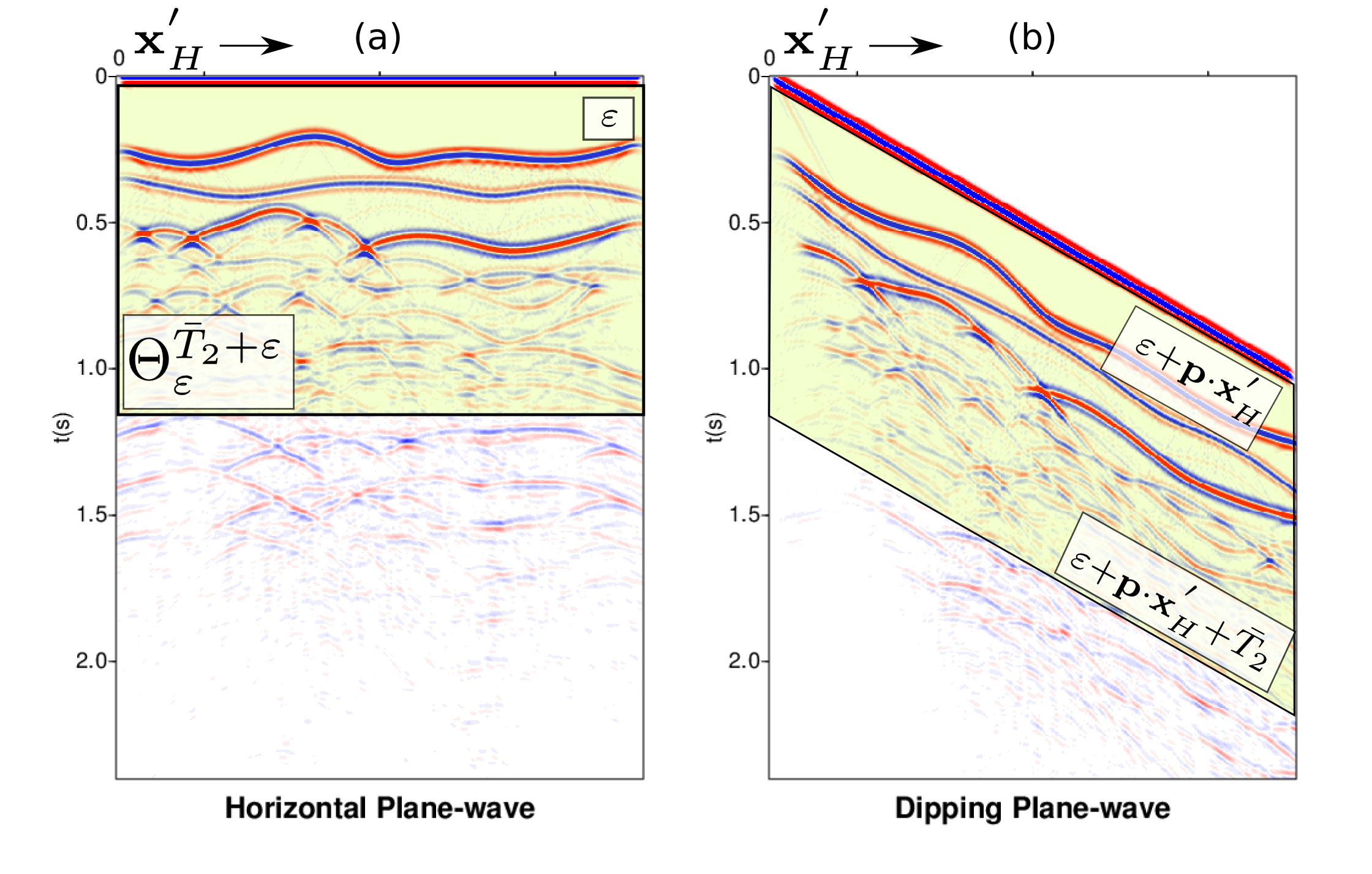
Figure 1: The shaded green areas show the support of representative muting operators for horizontal ($\Theta_{\varepsilon}^{\bar{T}_{2}+\varepsilon}$ in (a)) and dipping ($\Theta_{\varepsilon+\textbf{p}\cdot\textbf{x}_{H}^{{}^{\prime}}}^{\varepsilon+\bar{T}_{2}+\textbf{p}\cdot\textbf{x}_{H}^{{}^{\prime}}}$ in (b)) plane-wave sources (the corresponding data are shown in the background).

Figure 2: (a) Velocity and (b) density models used in the first numerical experiment.

Figure 3: (a) Full dataset associated with a plane-wave source fired at the surface of the model. Red arrows point at internal multiples. (b) Estimated primaries obtained by computing $\textbf{V}^{-}$ via Eq. 22 for all possible values $\bar{T}_{2}$ and storing results at $t=\bar{T}_{2}$. Differences in amplitude between gathers in (a) and (b) are due to multiple removal and transmission loss compensation.

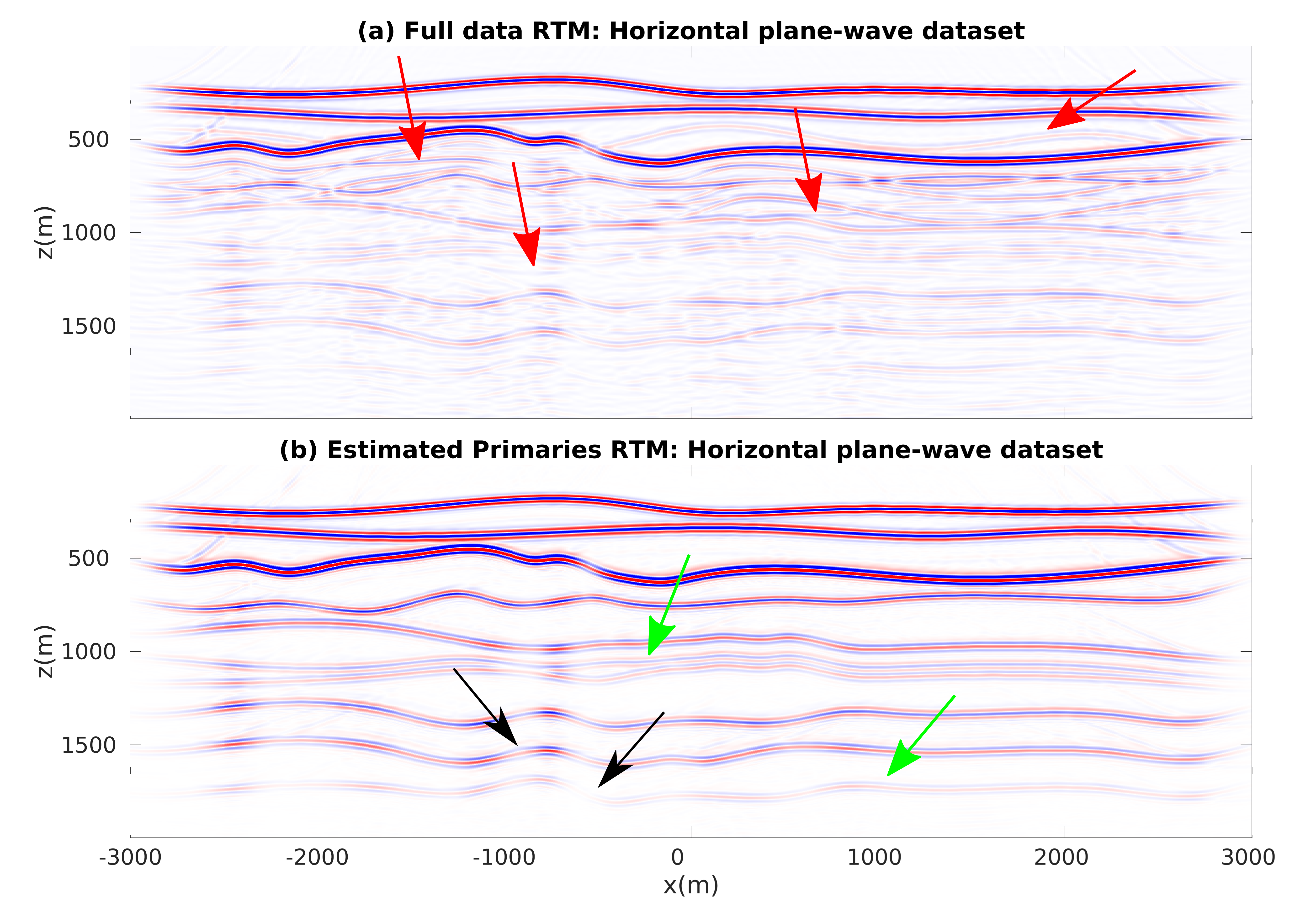
Figure 4: (a) Standard plane-wave reverse time migration of the dataset in Fig. 3(a). Red arrows point at artefacts related to internal multiples. (b) Standard plane-wave reverse time migration of the dataset in Fig. 3(b). Green arrows point at well resolved interfaces barely visible in (a) due to the superposition of internal multiples. Black arrows point at dipping interfaces only partially visible via horizontal plane-wave illumination. Differences in amplitude between images in (a) and (b) are due to multiple removal and transmission loss compensation.

For our first numerical experiment we consider a 2D model with gently dipping interfaces (see Fig. 2). The recording surface is reflection free. The dataset associated with a horizontal plane-wave source fired at the surface of this model is shown in Fig. 3(a). Notwithstanding the geometrical simplicity of the model, due to the strong impedance variations the data are contaminated with many internal multiples, as indicated by the red arrows. We then apply to this dataset the method as described in section 3.2. More precisely, we compute ${V}^{-}$ via Eq. 22 for all values $\bar{T}_{2}$, and by storing results at $t=\bar{T}_{2}$ we build a parallel dataset, which theoretically only involves primaries. Note that the algorithm is fully data driven, and no model information or any human intervention (e.g., picking) is involved in the process. For this dataset we only computed the first $20$ terms of the series in Eq. 22. The result of the procedure is shown in Fig. 3(b). We then image both datasets in Fig. 3 via standard plane-wave reverse time migration (based on the zero lag of the cross-correlation between the source and receiver wavefields, Claerbout, (1985)) using a smoothed version of the true velocity distribution in Fig. 2 and constant density. Migration results are shown in Fig. 4. When the full dataset is migrated, internal multiples contaminate the image as shown in Fig. 4(a), producing many false positive artefacts (indicated by red arrows). The image is much cleaner when the dataset in 3(b) is migrated. Each interface is properly recovered, as demonstrated by a comparison between Figs. 2 and 4(b). Green arrows in 4(b) point at physical interfaces which are invisible in Fig. 4(a), where they are attenuated by interfering multiple-related artefacts. Black arrows point at physical interfaces only partially resolved. The relatively poor performances in imaging dipping interfaces is not due to residual internal multiples, but to the intrinsic limitations of horizontal plane-wave imaging. However, note that only one demultipled plane-wave response and a single migration were required to produce the multiple-free image in Fig. 4(b). We conclude that for gently dipping models horizontal plane-wave datasets are sufficient to produce satisfactory results.

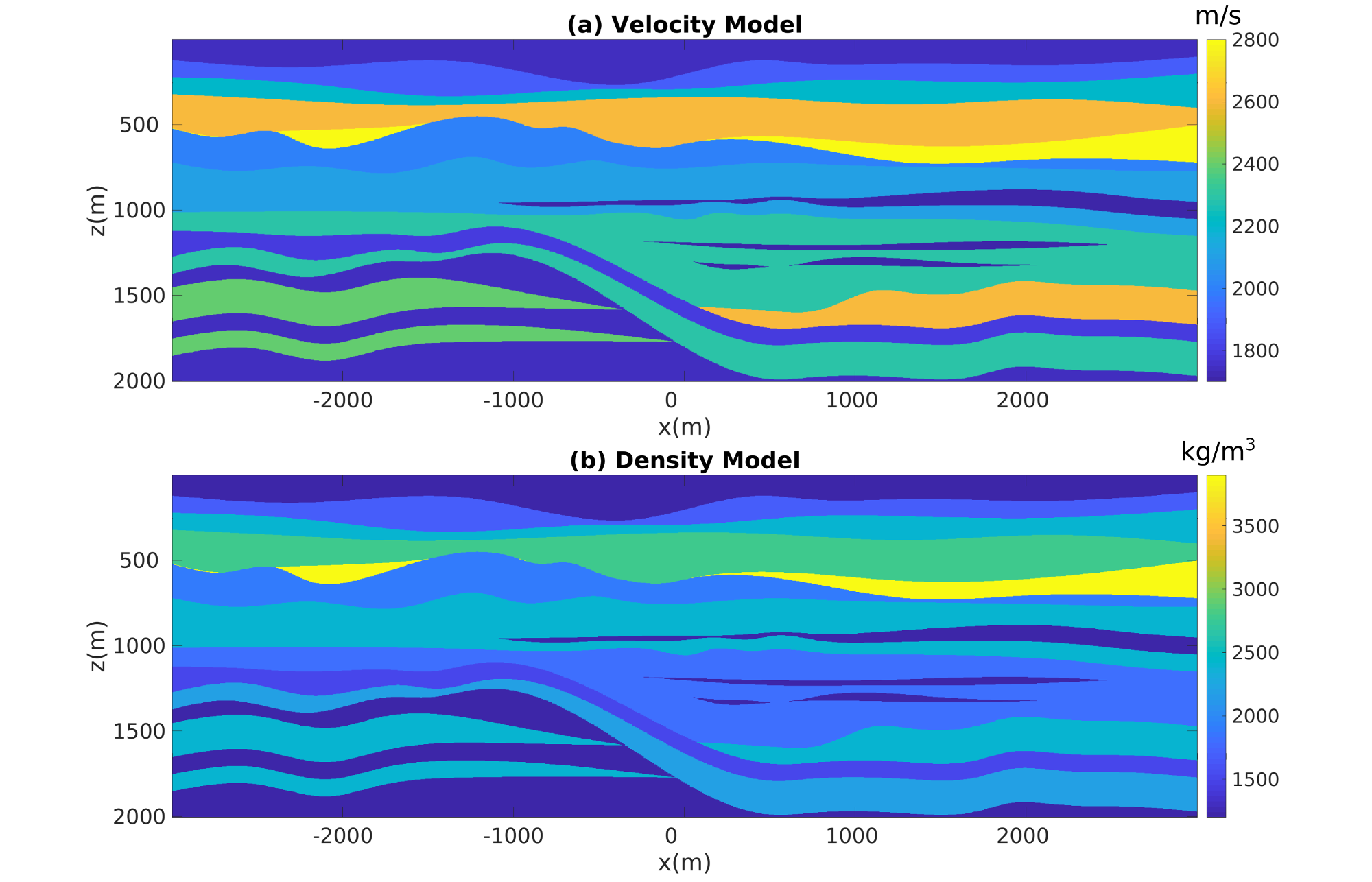
Figure 5: (a) Velocity and (b) density models used in the second numerical experiment.

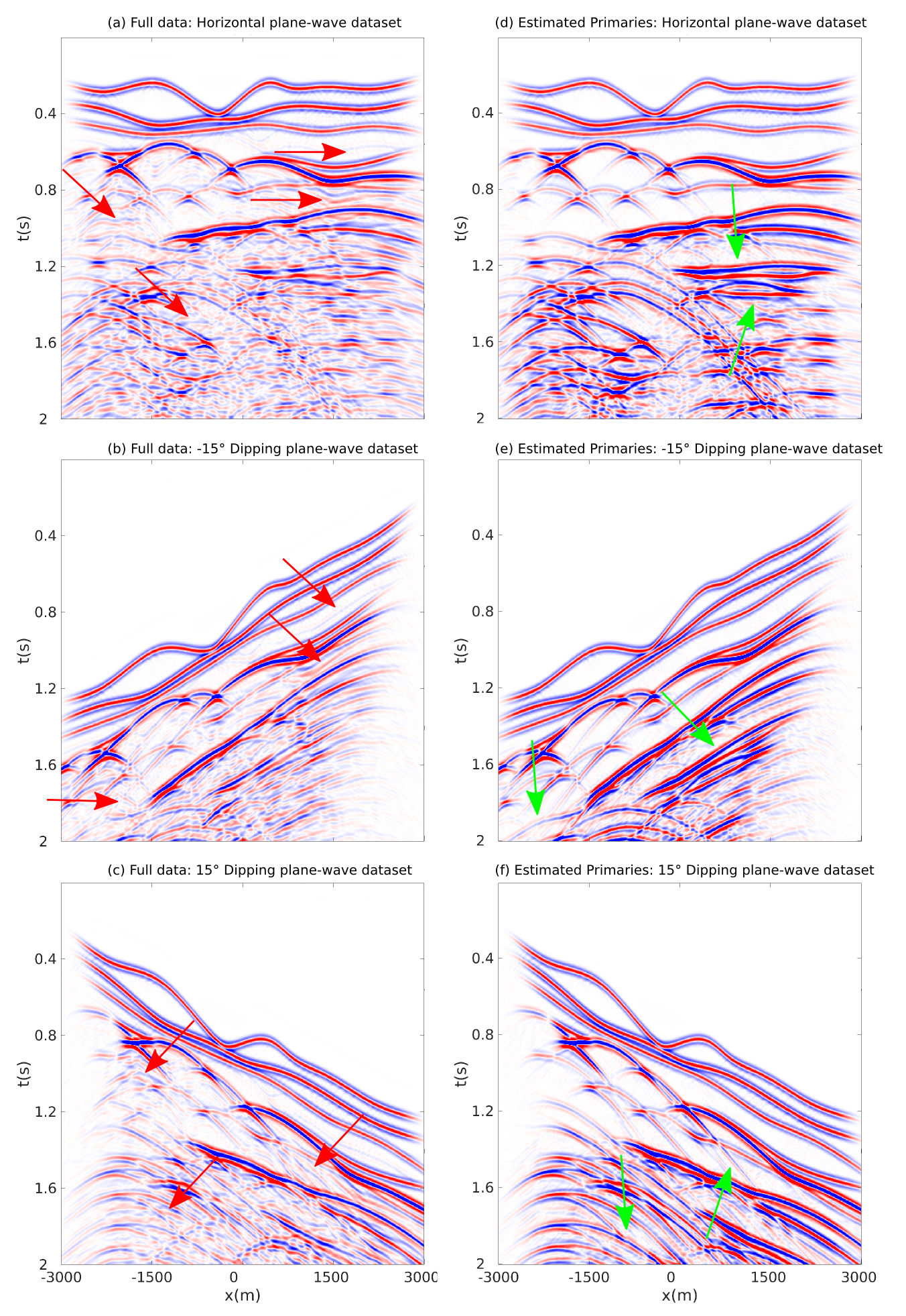
Figure 6: (a-c): reflection responses associated with plane wave sources at $-15^{\circ}$, $0^{\circ}$ and $15^{\circ}$, respectively. Red arrows show internal multiples. (d-f): estimated primaries associated with plane wave sources at $-15^{\circ}$, $0^{\circ}$ and $15^{\circ}$, respectively. Differences in amplitude between gathers in (a-c) and (d-f) are due to multiple removal and transmission loss compensation. Green arrows show primaries barely visible in the corresponding full datasets (a-c).

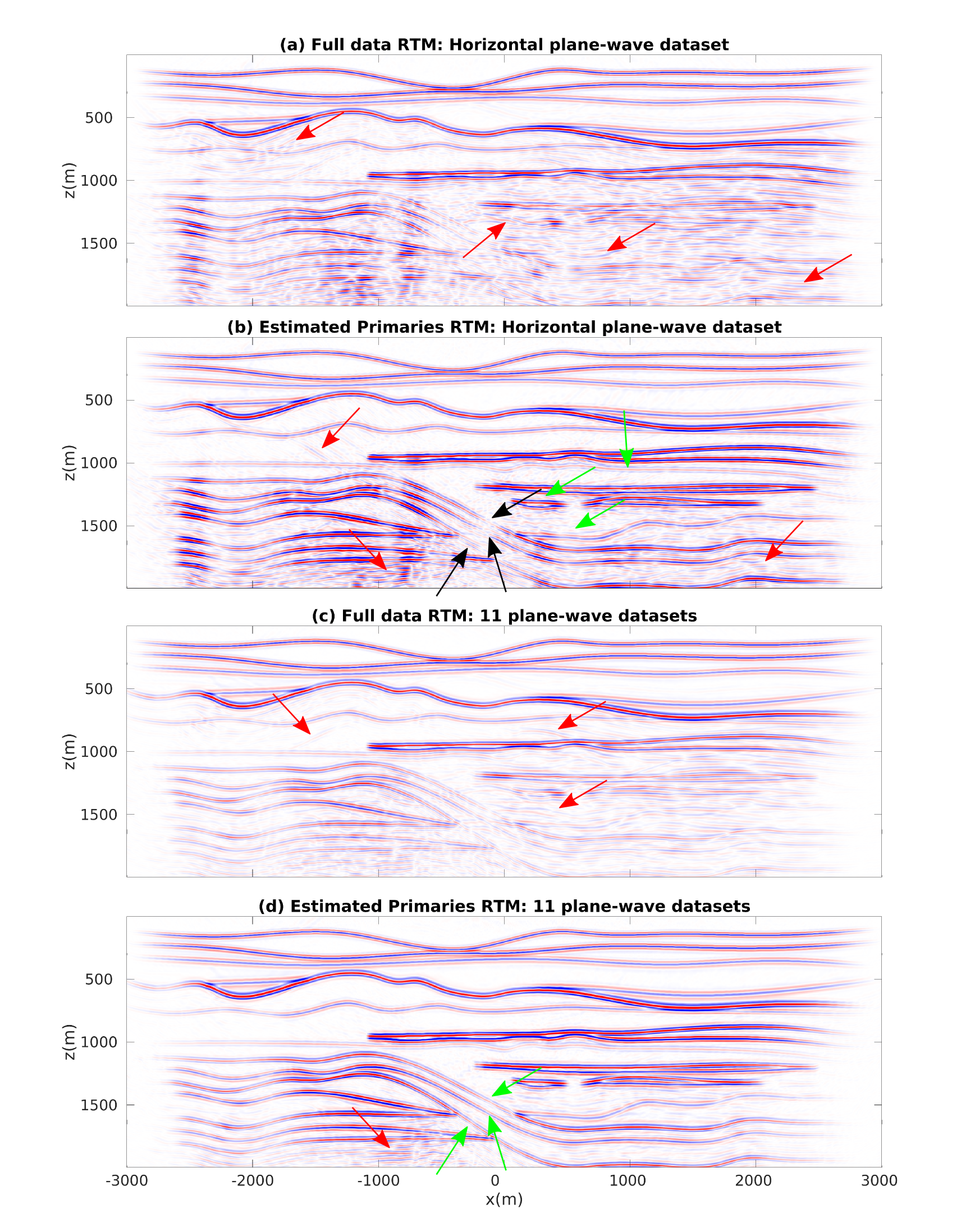
Figure 7: (a) Standard plane-wave reverse time migration of the dataset in Fig. 6(a). Red arrows point at artefacts related to internal multiples. (b) Standard plane-wave reverse time migration of the dataset in Fig. 6(b). Black arrows indicate dipping interfaces that are only partially recovered due to the poor illumination provided by a single plane-wave experiment. Note that these interfaces are also not properly imaged in (a). (c) Aggregate RTM of 11 plane wave full datasets (uniformly ranging from $-25^{\circ}$ to $25^{\circ}$). Red arrows point at artefacts related to internal multiples. (d) Aggregate Standard RTM of synthesized primaries. Green and red arrows indicate interfaces barely visible in (a) and minor residual artefacts, respectively. Differences in amplitude between images in (a,c) and (b,d) are due to multiples removal and transmission loss compensation (see Fig. 6).

In the second example (Fig. 5) we consider a more challenging model with critical features for any Marchenko method, i.e. the presence of thin layers, diffractors and dipping layers (Wapenaar et al., (2014); Zhang et al., 2019b ; Dukalski et al., (2019)). We initially follow the same imaging strategy as for the first example. We first compute the dataset associated with a horizontal plane-wave source fired at the surface of the model shown in Fig. 5(a). Also for this dataset we only computed the first $20$ terms of the series in Eq. 22. Given the complexity of the model, many events, primaries as well as internal multiples (red arrows) cross each-other, especially in the lower part of the plane-wave gather. Picking specific events in the gather in Fig. 6(a) would be challenging. However, as discussed above, our method does not involve any human intervention, and by applying the same scheme as for the first model we retrieve the dataset shown in Fig. 6(b), where primaries otherwise overshadowed by interfering multiples are clearly visible (green arrows). We then migrate datasets in Fig. 6(a) and (b), and show in Fig. 7(a) and (b) the corresponding images. Large portions of the image in Fig. 7(a) associated with the dataset in Fig. 6(a) are dominated by noise due to the presence of internal multiples (red arrows). On the other hand, the image in Fig. 7(b), which is associated with the estimated primaries in Fig. 6(d), is much cleaner, with fewer artefacts (red arrows) contaminating limited domains of the image. Note that relatively poor imaging performances of dipping interfaces (black arrows in Fig. 7(b)) are not necessarily associated with shortcomings of the discussed demultiple method but with the intrinsic limitation of what can be illuminated by a single plane-wave experiment. For this specific model we then decide to process and migrate also dipping plane-wave data. In total we then consider 10 additional datasets, uniformly ranging from $-25^{\circ}$ to $25^{\circ}$ (as discussed in section 3.3, the angle of the plane-wave is implemented by adding time delays to the shot positions on the horizontal array). Representative dipping plane-wave data are shown in Fig. 6(b,c), next to the corresponding processed gathers (in Fig. 6(e,f)). Red and green arrows point again at internal multiples and recovered primaries, respectively. We finally consider aggregate plane-wave migrated images. By migrating a total of $11$ full-data gathers, the image in Fig. 7(c) is obtained. While thanks to the better illumination the improvement over the image in Fig. 7(a) is clear, some of the key features of the final result are still misleading (red arrows point at false positives associated with the migration of internal multiples). A significantly better result is obtained when the $11$ processed gathers are imaged and stacked (Fig. 7(d)). The dipping features poorly visible in (b) are now properly resolved. This example shows that the proposed method can successfully process dipping plane-wave datasets and therefore benefit from the corresponding improved illumination. Residual artefacts in the migrated image indicated by the red arrow in Fig. 7(d) are likely due to the presence of thin layers, diffractors and dipping layers that are known to be critical in Marchenko methods.

5 Discussion

In section 3.2 we have extended a recently proposed primary synthesis method, devised for point source gathers, to horizontal plane-wave source data. The new scheme still needs full point-source data as input, but its output is a horizontal plane-wave response. The method is based on integration of point-source responses over the acquisition surface (e.g., Eqs. 9 and 10), which allows the derivation of relationships associated with plane-wave sources (e.g., Eqs. 17 and 18). Both the point-source and plane-wave primary synthesis methods are totally data driven, and both are implemented by inversion of the same family of linear operators, i.e.:

$${I}-\Theta_{\varepsilon}^{\bar{T}_{2}+\varepsilon}\textbf{R}\Theta_{\varepsilon}^{\bar{T}_{2}+\varepsilon}\textbf{R}^{\star}$$ (31)

Each operator is defined by a different value of $\bar{T}_{2}$. In previous literature that underlies this contribution, an integration over the focusing surface was used to adapt Greens’ functions redatuming methods to virtual plane-wave redatuming (Meles et al., (2018)). While conceptually similar, there is a subtle yet very important difference between the methods discussed here and previous methods on virtual plane-wave redatuming. Whereas in any Marchenko redatuming scheme (e.g. for point or plane virtual sources) a different, model dependent, window operator for each point or plane is required, as focusing is achieved in the subsurface, the window operators discussed here are the same for each input data, as the focusing operators are projected to the surface. Since the operators in Eq. 31 are linear and do not depend on the specific gather they are applied to, any linear combination of point-source data can be processed at once, provided that all the corresponding sources are fired at the same time (see section 3.2 for more details). The proposed method can then be used, without any modification, to blended-source data as well as to individual point sources and horizontal plane-wave gathers. This is shown in Fig. 8, where the algorithm is applied to a dataset associated with 5 sources with different spectra fired at the same time (Fig. 8(a)). Application of the proposed scheme results in the gather shown in Fig. 8(b). A nearly identical result (relative difference smaller than $0.1\%$) is achieved when the method is applied to each single point source gather separately, after which the corresponding results are summed together.
In section 3.3 we extended the primary synthesis method for dipping plane-wave source data, which helps to improve the illumination of dipping interfaces in the subsurface.

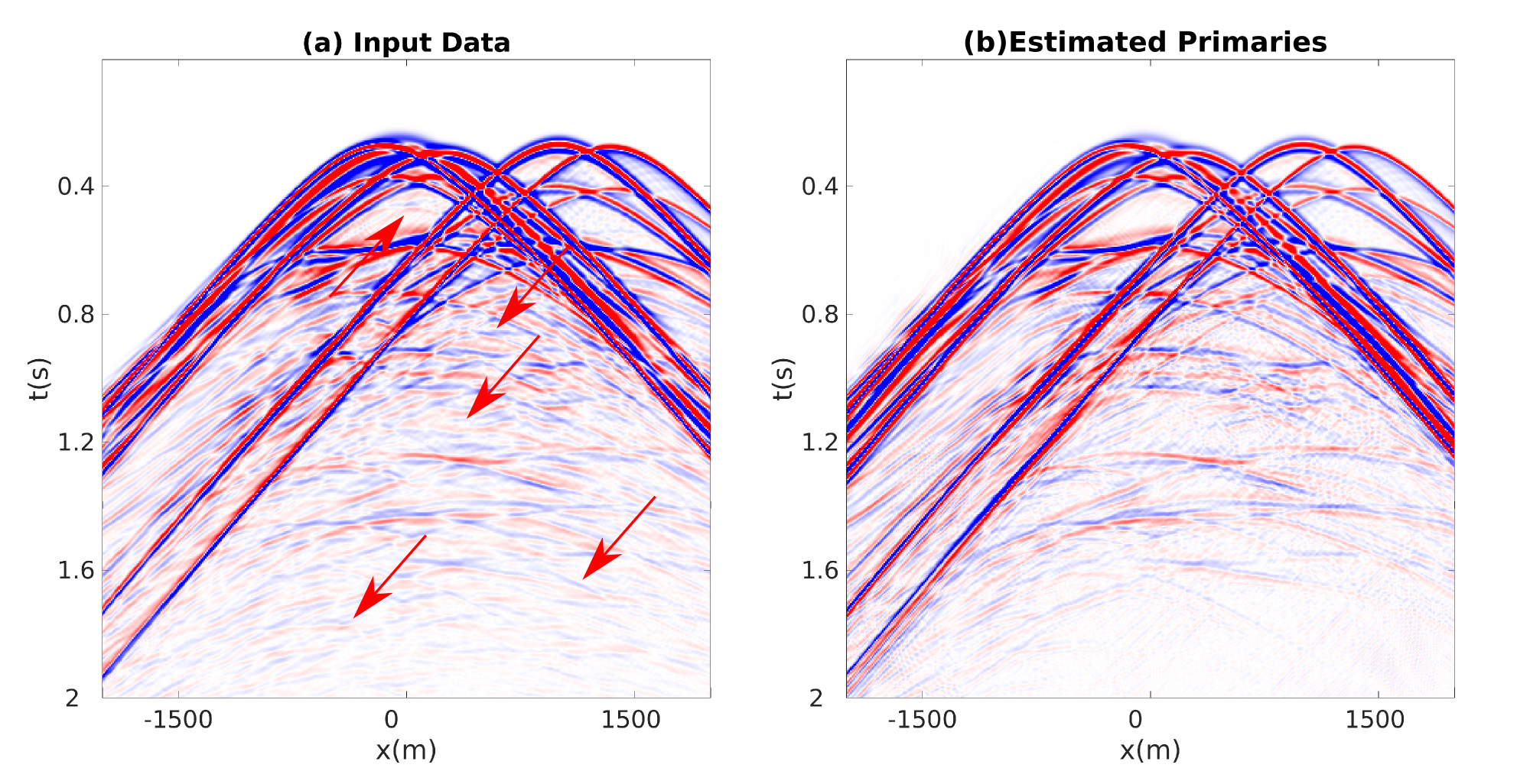
Figure 8: (a) Full dataset associated with 5 point sources with different spectrum content fired at the same time. Red arrows point at internal multiples. (b) Corresponding estimated primaries.

6 Conclusions

We have shown that recent advances in data domain Marchenko methods can be extended to incorporate plane-wave source concepts. More specifically, we have discussed how to retrieve estimates of the primary responses to a plane-wave source. The retrieved primaries can then be used via standard reverse time migration to produce images free of artefacts related to internal multiples. Whereas previous data domain Marchenko methods are applied to point source gathers and therefore tend to be rather expensive for large datasets, the proposed method provides good imaging results by only involving a small number of primary synthesis steps and the corresponding plane-wave reverse time migration. The plane-wave source primary synthesis algorithm discussed in this paper could then be used as an initial and inexpensive processing step, potentially guiding more expensive target imaging techniques. In this paper we have only discussed 2D examples and internal multiples, but an obvious extension would be allowing surface source primary synthesis in 3D problems as well as incorporating free surface multiples. Finally, applications of data domain Marchenko methods to field data have already been performed. Future work will then focus on applying plane-wave primary synthesis methods to field data too.

Data and materials availability

The data that support the findings of this study are available from the corresponding author upon request.

References

- Becker et al., (2018) Becker, T. S., Ravasi, M., Broggini, F., Robertsson, J. O., et al. (2018). Sparse inversion of the coupled Marchenko equations for simultaneous source wavelet and focusing functions estimation. In 80th EAGE Conference and Exhibition 2018, number Th P9 15.
- Behura and Snieder, (2013) Behura, J. and Snieder, R. (2013). Imaging direct as well as scattered events in microseismic data using inverse scattering theory. In SEG Technical Program Expanded Abstracts 2013, pages 2019–2023. Society of Exploration Geophysicists.
- Brackenhoff et al., (2019) Brackenhoff, J., Thorbecke, J., and Wapenaar, K. (2019). Monitoring of induced distributed double-couple sources using Marchenko-based virtual receivers. Solid Earth, 10:1301–1319.
- Broggini et al., (2012) Broggini, F., Snieder, R., and Wapenaar, K. (2012). Focusing the wavefield inside an unknown 1D medium: Beyond seismic interferometry. Geophysics, 77(5):A25–A28.
- Broggini et al., (2014) Broggini, F., Snieder, R., and Wapenaar, K. (2014). Data-driven wavefield focusing and imaging with multidimensional deconvolution: Numerical examples for reflection data with internal multiples. Geophysics, 79(3):WA107–WA115.
- Claerbout, (1985) Claerbout, J. F. (1985). Imaging the Earth’s interior. Blackwell scientific publications Oxford.
- (7) da Costa Filho, C., Meles, G., Curtis, A., Ravasi, M., and Kritski, A. (2017a). Imaging strategies using focusing functions with applications to a North Sea field. Geophysical Journal International, 213(1):561–573.
- (8) da Costa Filho, C. A., Meles, G. A., and Curtis, A. (2017b). Elastic internal multiple analysis and attenuation using Marchenko and interferometric methods. Geophysics, 82(2):Q1–Q12.
- da Costa Filho et al., (2014) da Costa Filho, C. A., Ravasi, M., Curtis, A., and Meles, G. A. (2014). Elastodynamic Green’s function retrieval through single-sided Marchenko inverse scattering. Physical Review E, 90(6):063201.
- Dai and Schuster, (2013) Dai, W. and Schuster, G. T. (2013). Plane-wave least-squares reverse-time migration. Geophysics, 78(4):S165–S177.
- Dragoset et al., (2010) Dragoset, B., Verschuur, E., Moore, I., and Bisley, R. (2010). A perspective on 3D surface-related multiple elimination. Geophysics, 75(5):75A245–75A261.
- Dukalski et al., (2019) Dukalski, M., Mariani, E., and de Vos, K. (2019). Handling short-period scattering using augmented Marchenko autofocusing. Geophysical Journal International, 216(3):2129–2133.
- Fokkema and van den Berg, (1993) Fokkema, J. T. and van den Berg, P. M. (1993). Seismic applications of acoustic reciprocity. Elsevier.
- Gray et al., (2001) Gray, S. H., Etgen, J., Dellinger, J., and Whitmore, D. (2001). Seismic migration problems and solutions. Geophysics, 66(5):1622–1640.
- Jakubowicz, (1998) Jakubowicz, H. (1998). Wave equation prediction and removal of interbed multiples. In SEG Technical Program Expanded Abstracts 1998, pages 1527–1530. Society of Exploration Geophysicists.
- Jia et al., (2018) Jia, X., Guitton, A., and Snieder, R. (2018). A practical implementation of subsalt Marchenko imaging with a Gulf of Mexico data set. Geophysics, 83(5):S409–S419.
- Kelamis et al., (2006) Kelamis, P. G., Zhu, W., Rufaii, K. O., and Luo, Y. (2006). Land multiple attenuation—the future is bright. In SEG Technical Program Expanded Abstracts 2006, pages 2699–2703. Society of Exploration Geophysicists.
- Löer et al., (2016) Löer, K., Curtis, A., and Meles, G. A. (2016). Relating source-receiver interferometry to an inverse-scattering series to derive a new method to estimate internal multiples. Geophysics, 81(3):Q27–Q40.
- McMechan, (1983) McMechan, G. A. (1983). p-x imaging by localized slant stacks of t-x data. Geophysical Journal International, 72(1):213–221.
- Meles et al., (2015) Meles, G. A., Löer, K., Ravasi, M., Curtis, A., and da Costa Filho, C. A. (2015). Internal multiple prediction and removal using Marchenko autofocusing and seismic interferometry. Geophysics, 80(1):A7–A11.
- Meles et al., (2019) Meles, G. A., van der Neut, J., van Dongen, K. W. A., and Wapenaar, K. (2019). Wavefield finite time focusing with reduced spatial exposure. The Journal of the Acoustical Society of America, 145(6):3521–3530.
- Meles et al., (2018) Meles, G. A., Wapenaar, K., and Thorbecke, J. (2018). Virtual plane-wave imaging via Marchenko redatuming. Geophysical Journal International, 214(1):508–519.
- Mulder and Plessix, (2004) Mulder, W. A. and Plessix, R.-E. (2004). A comparison between one-way and two-way wave-equation migration. Geophysics, 69(6):1491–1504.
- Ravasi, (2017) Ravasi, M. (2017). Rayleigh-Marchenko redatuming for target-oriented, true-amplitude imaging. Geophysics, 82(6):S439–S452.
- Ravasi et al., (2016) Ravasi, M., Vasconcelos, I., Kritski, A., Curtis, A., da Costa, C. A., and Meles, G. A. (2016). Target-oriented Marchenko imaging of a North Sea field. Geophysical Journal International, 205(1):99–104.
- Reinicke and Wapenaar, (2019) Reinicke, C. and Wapenaar, K. (2019). Elastodynamic single-sided homogeneous Green’s function representation: Theory and numerical examples. Wave Motion, 89:245–264.
- Rietveld et al., (1992) Rietveld, W., Berkhout, A., and Wapenaar, C. P. A. (1992). Optimum seismic illumination of hydrocarbon reservoirs. Geophysics, 57(10):1334–1345.
- Schultz and Claerbout, (1978) Schultz, P. S. and Claerbout, J. F. (1978). Velocity estimation and downward continuation by wavefront synthesis. Geophysics, 43(4):691–714.
- Slob and Wapenaar, (2014) Slob, E. and Wapenaar, K. (2014). Data-driven inversion of gpr surface reflection data for lossless layered media. In The 8th European Conference on Antennas and Propagation (EuCAP 2014), pages 3378–3382. IEEE.
- Slob and Wapenaar, (2017) Slob, E. and Wapenaar, K. (2017). Theory for Marchenko imaging of marine seismic data with free surface multiple elimination. In 79th EAGE Conference and Exhibition 2017.
- Slob et al., (2014) Slob, E., Wapenaar, K., Broggini, F., and Snieder, R. (2014). Seismic reflector imaging using internal multiples with Marchenko-type equations. Geophysics, 79(2):S63–S76.
- Staring et al., (2018) Staring, M., Pereira, R., Douma, H., van der Neut, J., and Wapenaar, K. (2018). Source-receiver Marchenko redatuming on field data using an adaptive double-focusing method. Geophysics, 83(6):S579–S590.
- Stoffa et al., (2006) Stoffa, P. L., Sen, M. K., Seifoullaev, R. K., Pestana, R. C., and Fokkema, J. T. (2006). Plane-wave depth migration. Geophysics, 71(6):S261–S272.
- ten Kroode, (2002) ten Kroode, F. (2002). Prediction of internal multiples. Wave Motion, 35(4):315–338.
- Thorbecke et al., (2017) Thorbecke, J., Slob, E., Brackenhoff, J., van der Neut, J., and Wapenaar, K. (2017). Implementation of the Marchenko method. Geophysics, 82(6):WB29–WB45.
- van Borselen, (2002) van Borselen, R. (2002). Fast-track, data-driven interbed multiple removal-a North Sea data example. In 64th EAGE Conference & Exhibition, number F-40.
- van der Neut and Fokkema, (2018) van der Neut, J. and Fokkema, J. (2018). One-dimensional Marchenko inversion in stretched space. In Proceedings of the International Workshop on Medical Ultrasound Tomography: 1.-3. Nov. 2017, Speyer, Germany, pages 15–24. KIT Scientific Publishing.
- van der Neut et al., (2017) van der Neut, J., Johnson, J. L., van Wijk, K., Singh, S., Slob, E., and Wapenaar, K. (2017). A Marchenko equation for acoustic inverse source problems. The Journal of the Acoustical Society of America, 141(6):4332–4346.
- (39) van der Neut, J., Vasconcelos, I., and Wapenaar, K. (2015a). On Green’s function retrieval by iterative substitution of the coupled Marchenko equations. Geophysical Journal International, 203(2):792–813.
- van der Neut and Wapenaar, (2016) van der Neut, J. and Wapenaar, K. (2016). Adaptive overburden elimination with the multidimensional Marchenko equation. Geophysics, 81(5):T265–T284.
- (41) van der Neut, J., Wapenaar, K., Thorbecke, J., and Slob, E. (2015b). Practical challenges in adaptive Marchenko imaging. In SEG Technical Program Expanded Abstracts 2015, pages 4505–4509. Society of Exploration Geophysicists.
- Wang et al., (2018) Wang, X., Ji, X., Liu, H., and Luo, Y. (2018). Fast plane-wave reverse time migration. Geophysics, 83(6):S549–S556.
- Wapenaar et al., (2018) Wapenaar, K., Brackenhoff, J., Thorbecke, J., van der Neut, J., Slob, E., and Verschuur, E. (2018). Virtual acoustics in inhomogeneous media with single-sided access. Scientific Reports, 8(1):2497.
- Wapenaar et al., (2012) Wapenaar, K., Broggini, F., and Snieder, R. (2012). Creating a virtual source inside a medium from reflection data: heuristic derivation and stationary-phase analysis. Geophysical Journal International, 190(2):1020–1024.
- Wapenaar et al., (2014) Wapenaar, K., Thorbecke, J., van der Neut, J., Broggini, F., Slob, E., and Snieder, R. (2014). Marchenko imaging. Geophysics, 79(3):WA39–WA57.
- Weglein et al., (1997) Weglein, A. B., Gasparotto, F. A., Carvalho, P. M., and Stolt, R. H. (1997). An inverse-scattering series method for attenuating multiples in seismic reflection data. Geophysics, 62(6):1975–1989.
- Whitmore, (1983) Whitmore, N. D. (1983). Iterative depth migration by backward time propagation. In SEG Technical Program Expanded Abstracts 1983, pages 382–385. Society of Exploration Geophysicists.
- Wiggins, (1988) Wiggins, J. W. (1988). Attenuation of complex water-bottom multiples by wave-equation-based prediction and subtraction. Geophysics, 53(12):1527–1539.
- Yilmaz, (2001) Yilmaz, Ö. (2001). Seismic data analysis: Processing, inversion, and interpretation of seismic data. Society of Exploration Geophysicists.
- Zhang and Slob, (2019) Zhang, L. and Slob, E. (2019). Free-surface and internal multiple elimination in one step without adaptive subtraction. Geophysics, 84(1):A7–A11.
- (51) Zhang, L. and Slob, E. (2020a). A fast algorithm for multiple elimination and transmission compensation in primary reflections. Geophysical Journal International. ggaa005.
- (52) Zhang, L. and Slob, E. (2020b). A field data example of Marchenko multiple elimination. Geophysics, 85(2):S65–S70.
- Zhang and Staring, (2018) Zhang, L. and Staring, M. (2018). Marchenko scheme based internal multiple reflection elimination in acoustic wavefield. Journal of Applied Geophysics, 159:429–433.
- (54) Zhang, L., Thorbecke, J., Wapenaar, K., and Slob, E. (2019a). Data-driven internal multiple elimination and its consequences for imaging: A comparison of strategies. Geophysics, 84(5):S365–S372.
- (55) Zhang, L., Thorbecke, J., Wapenaar, K., and Slob, E. (2019b). Transmission compensated primary reflection retrieval in data domain and consequences for imaging. Geophysics, 84(4):Q27–Q36.
- Zhu et al., (1998) Zhu, J., Lines, L., and Gray, S. (1998). Smiles and frowns in migration/velocity analysis. Geophysics, 63(4):1200–1209.