Uncertainty-Aware Anticipation of Activities

Abstract

Anticipating future activities in video is a task with many practical applications. While earlier approaches are limited to just a few seconds in the future, the prediction time horizon has just recently been extended to several minutes in the future. However, as increasing the predicted time horizon, the future becomes more uncertain and models that generate a single prediction fail at capturing the different possible future activities. In this paper, we address the uncertainty modelling for predicting long-term future activities. Both an action model and a length model are trained to model the probability distribution of the future activities. At test time, we sample from the predicted distributions multiple samples that correspond to the different possible sequences of future activities. Our model is evaluated on two challenging datasets and shows a good performance in capturing the multi-modal future activities without compromising the accuracy when predicting a single sequence of future activities.

1 Introduction

Anticipating future activities in video has become an active research topic in computer vision. While earlier approaches focused on early activity detection [20, 6, 13, 21], recent models predict activities a few seconds in the future [12, 7, 24, 4]. However, predicting the future activity label shortly before it starts is not sufficient for many applications. Robots, for instance, that interact with humans to accomplish industrial tasks or help in housework need to anticipate activities for a long time horizon. Such long-term prediction would enable these robots to plan ahead to complete their tasks efficiently. Moreover, anticipating the activities of other interacting humans improves human-robot interaction.

Recently, [1] extended the prediction horizon to a few minutes in the future and predict both future activities and their durations as well. While their approach generates good predictions, it does not take the uncertainty of the future into consideration. For example, given a video snippet that shows a person taking a cup from the cupboard, we cannot be sure whether the future activity would be pour water or pour coffee. Approaches that predict a single output and do not model the uncertainty in the future actions would fail in such cases. On the contrary, approaches that are capable of predicting all the possible outputs are preferable. Fig. 1 illustrates a case where the future activities have multiple modes and the model has to predict all these modes.

In this paper, we introduce a framework that models the probability distribution of the future activities and use this distribution to generate several possible sequences of future activities at test time. To this end, we train an action model that predicts a probability distribution of the future action label, and a length model which predicts a probability distribution of the future action length. At test time, we sample from these models a future action segment represented by an action label and its length. To predict more in the future, we feed the predicted action segment to the model and predict the next one recursively. We evaluate our framework on two datasets with videos of varying length and many action segments: the Breakfast dataset [11] and 50Salads [23]. Our framework outperforms a baseline that predicts the future activities using n-grams as an action model and a Gaussian to predict the action length. Furthermore, we are able to achieve results that are comparable with the state-of-the-art if we use the framework to predict a single sequence of future activities.

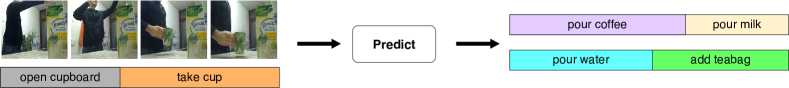
Figure 1: The anticipation task. Given an observed part of a video, we want to predict the future activities that might follow in the future with their durations. The model outputs a collection of samples to represent the uncertainty in the future actions.

2 Related Work

Future prediction has been studied by many researchers. However, the predicted time horizon is very limited in earlier approaches. Instead of predicting the future, Hoai and De la Torre [6] proposed a max-margin framework for early activity detection. Other approaches adapt special loss functions to detect a partially observed activity [13, 21]. To predict future actions, Lan et al. [12] proposed hierarchical representations of short clips or still images. In [10] a spatio-temporal graph is used to predict object affordances, trajectories, and sub-activities. Vondrick et al. [24] trained a deep convolutional neural network to predict features in the future from a single frame. An SVM is then used to predict the future action label from the predicted features. In [4], a sequence of visual representations of past frames is used to predict a sequence of future representations. A reinforcement learning module is used to provide supervision at sequence level. Zeng et al. [25] used inverse reinforcement learning to anticipate visual representations from unlabeled video. Shi et al. [22] proposed a recurrent neural network with radial basis function kernels to predict features in the future and then predict the action label with a multi-layer perceptron. Instead of features, [19] predict future dynamic images and train a classifier to predict the action label on top of the predicted images. Furnari et al. [3] predict future actions in egocentric videos and evaluate the top-k accuracy to consider the multi-modal future. Miech et al. [16] combine a predictive model that directly predicts the future action label with a transitional model that models the transition probabilities between actions. However, all of the previous approaches predict an action label without any time information. Heidarivincheh et al. [5] introduced a model to predict the time of completion for an observed activity. In [14], both the future activity and its starting time are predicted.

Despite the success of the previous approaches in predicting the future actions, they are however limited to a few seconds in the future. For many real world applications, a long-term prediction beyond just a few seconds is crucial. Recently, Abu Farha et al. [1] introduced a two-step approach that is capable of anticipating future activities several minutes in the future. Given an observed part of a video, they infer the activities in the observed part first and then anticipate the future activities and their durations. For the anticipation step, both an RNN and a CNN are trained to generate the future action segments. Ke et al. [8] build on this two-step framework and use temporal convolutions with attention to anticipate future activities. The model output is conditioned on a time parameter to determine the predicted time horizon. In contrast to these approaches, we predict multiple outputs to consider the uncertainty in the future activities. In a very recent work, [15] adapt a variational auto-encoder framework to predict a distribution over the future action and its starting time. However, they do not model the dependency between the future action and its starting time directly and rely on a shared latent space to capture this dependency. On the contrary, our framework directly models the dependency between the action label and its length.

3 Anticipating Activities

Given an observed part of a video with $n$ action segments $c_{1:n}=(c_{1},\dots,c_{n})$ with length $l_{1:n}=(l_{1},\dots,l_{n})$, we want to predict all the action segments and their lengths that will occur in the future unseen part of that video. I.e. we want to predict the segments $c_{n+1:N}$ and the corresponding segments length $l_{n+1:N}$, where $N$ is the total number of action segments in the video. Furthermore, since the last observed action segment $c_{n}$ might be partially observed and will continue in the future, we want to update our estimate of $l_{n}$ as well. Since for the same observed action segments $c_{1:n}$ there are more than one possible future action segments, we want to predict more than one output to capture the different modes in the future as shown in Fig. 1. To this end, we propose a framework to model the uncertainty in the future activities, and then use this framework to generate samples of the future action segments. We start with the model description in Section 3.1, and then describe the prediction procedure in Section 3.2.

3.1 Model

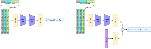
		(a)	(b)

Figure 2: Our anticipation framework consists of: (a) The action model which predicts the probability distribution of the future action label. (b) The length model which predicts the probability distribution of the future action length.

We follow the two-step approach proposed in [1] and infer the actions in the observed frames and then predict the future actions. For inferring the actions in the observed part, we use the same RNN-HMM model [18] that is used by [1]. Our goal now is to model the probability of the future actions and their lengths. This can be done using an autoregressive model that predicts the future action and its length, and then feeding the predicted output to the model again to predict the next one. Using such an autoregressive approach allows us to use the same model to predict actions for arbitrarily long time horizons. The probability distribution of the future action segment and its length can be factorized as follows

$$\begin{split}p(c_{n+1},\ l_{n+1}|c_{1:n},\ l_{1:n})=p(c_{n+1}|c_{1:n},\ l_{1:n})\ \cdot\\ p(l_{n+1}|c_{1:n},\ l_{1:n},\ c_{n+1}),\end{split}$$ (1)

where the first factor $p(c_{n+1}|c_{1:n},\ l_{1:n})$ is an action model that describes the probability distribution of the future action label given the preceding action segments. Whereas the second factor $p(l_{n+1}|c_{1:n},\ l_{1:n},\ c_{n+1})$ is a length model that describes the probability distribution of the future action length given the preceding action segments and the future action label. In the following, we discuss the details of these models.

3.1.1 Action Model

The action model predicts a probability distribution of the future action given the sequence of observed action segments and their lengths. For this model we use an RNN-based model similar to the one proposed in [1] as shown in Fig. 2 (a). Given the observed part of the video, each action segment is represented by a vector of a 1-hot encoding of the action label and the corresponding segment length. This sequence is passed through a fully connected layer, two layers of gated recurrent units (GRUs), and another fully connected layer. We use ReLU activations for the fully connected layers. For the output layer, we use another fully connected layer that predicts action scores for the future action. To get the probability distribution of the future action, we apply a softmax over the predicted scores

$$p(c_{n+1}=\hat{c}|c_{1:n},\ l_{1:n})=\frac{e^{x_{\hat{c}}}}{\sum_{\tilde{c}}e^{x_{\tilde{c}}}},$$ (2)

where $x_{\hat{c}}$ is the predicted action score for the class $\hat{c}$. To train this model, we use a cross entropy loss

$$\mathcal{L}_{action}=\frac{1}{M}\sum_{m}-log(y_{m,c}),$$ (3)

where $y_{m,c}$ is the predicted probability for the ground-truth future action label $c$ in the $m^{th}$ training example.

3.1.2 Length Model

We model the probability distribution of the future action length with a Gaussian distribution, i.e.

$$p(l_{n+1}|c_{1:n},\ l_{1:n},\ c_{n+1})=\mathcal{N}(\mu,\ \sigma^{2}).$$ (4)

To predict the mean length $\mu$ and the standard deviation $\sigma$ of this distribution, we use a network with two branches as shown in Fig. 2 (b). The first branch is the same as the RNN-based model used in the action model. It takes the sequence of the observed action segments as input and encodes them into a single vector representation. Whereas the second branch is a single fully connected layer that takes a 1-hot encoding of the future action $c_{n+1}$ and encodes it in another single vector representation. These two encoded vectors are concatenated and passed through two fully connected output layers to predict the mean length $\mu$ and the standard deviation $\sigma$. To ensure that the standard deviation is non-negative we use exponential activations for the output layer. To train the length model, we minimize the negative log likelihood of the target length

$$\begin{split}\mathcal{L}_{length}&=\frac{1}{M}\sum_{m}-log\ p(l_{n+1}=\ell_{m}|c_{1:n},\ l_{1:n},\ c_{n+1}),\\ &=\frac{1}{M}\sum_{m}0.5\ log(2\pi)\ +log(\sigma_{m})\ +\\ &\quad\ \ \frac{(\ell_{m}\ -\ \mu_{m})^{2}}{2\sigma_{m}^{2}},\end{split}$$ (5)

where $\ell_{m}$ is the ground-truth length of the future action, $\mu_{m}$ and $\sigma_{m}$ are the predicted mean length and standard deviation for the $m^{th}$ training example. As the first term in (5) is constant, our final loss function for the length model can be reduced to

$$\mathcal{L}_{length}=\frac{1}{M}\sum_{m}log(\sigma_{m})\ +\frac{(\ell_{m}\ -\ \mu_{m})^{2}}{2\sigma_{m}^{2}}.$$ (6)

The training examples for both the action and length models are generated based on the ground-truth segmentation of the training videos. Given a video with $n$ action segments, we generate $n-1$ training examples. For a segment $i>1$, the sequence of all the preceding segments is considered as input of the training example, where each segment is represented by a vector of a 1-hot encoding of the action label and the corresponding segment length. The action label of segment $i$ defines the target for the action model and its length serves as a target for the length model.

3.2 Prediction

Given an observed part of a video with $n$ action segments, we want to generate plausible sequences of future activities. Note that the observed part might end in a middle of an action segment and the last segment in the observations might be not fully observed. In the following we describe two strategies for predicting the sequence of future activities. The first strategy generates multiple sequences of activities by sampling from the predicted distributions of our approach. Whereas the second strategy is used to generate a single prediction that corresponds to the mode of the predicted distributions.

3.2.1 Prediction by Generating Samples

At test time we alternate between two steps: sampling a future action label from the action model

$$\hat{c}_{n+1}\sim p(c_{n+1}|c_{1:n},\ l_{1:n}),$$ (7)

and then we sample a length for the sampled future action using the length model

$$\hat{l}_{n+1}\sim p(l_{n+1}|c_{1:n},\ l_{1:n},\ \hat{c}_{n+1}).$$ (8)

We feed the predicted action segment recursively to the model until we predict the desired time horizon. As the last observed action segment might continue in the future, we start the prediction with updating the length of the last observed action segment. For this step, we sample a length for the last observed action segment based on the preceding segments and only update the length of that segment if the generated sample is greater than the observed length as follows

$$\hat{l}_{n}\sim p(l_{n}|c_{1:n-1},\ l_{1:n-1},\ c_{n}),$$ (9)

$$l_{n}^{\star}=\begin{cases}\hat{l}_{n}&:\hat{l}_{n}>\ell_{n}\\ \ell_{n}&:otherwise\\ \end{cases},$$ (10)

where $\ell_{n}$ is the observed length of the last observed action segment, and $l_{n}^{\star}$ is the predicted full length of that segment.

3.2.2 Prediction of the Mode

For predicting the mode, we also alternate between predicting the future action label and then predicting the length of that label. However, instead of sampling from the predicted action distribution, we choose the action label with the highest probability. For predicting the length, we use the predicted mean length from the length model instead of sampling from the predicted distribution.

3.3 Implementation Details

We implemented both models in PyTorch [17] and trained them using Adam optimizer [9] with a learning rate of $0.001$. The batch size is set to $32$. We trained the action model for $60$ epochs and the length model is trained for $30$ epochs. Dropout is used after each layer with probability $0.5$. We also apply standardization to the length of the action segments as follows

$$l=\frac{l-\overline{l}}{\sigma_{l}},$$ (11)

where $\overline{l}$ and $\sigma_{l}$ are the mean length and standard deviation, respectively, computed from the lengths of all action segments in the training videos.

4 Experiments

Datasets.

We evaluate the proposed model on two challenging datasets: the Breakfast dataset [11] and 50Salads [23].

The Breakfast dataset contains $1,712$ videos with roughly $3.6$ million frames. Each video belongs to one out of ten breakfast related activities, such as make tea or pancakes. The video frames are annotated with fine-grained action labels like pour water or take cup. Overall, there are $48$ different actions where each video contains $6$ action instances on average. The videos were recorded by $52$ actors in 18 different kitchens with varying view points. For evaluation, we use the standard 4 splits as proposed in [11] and report the average.

The 50Salads dataset contains 50 videos with roughly $600,000$ frames. On average, each video contains $20$ action instances and is $6.4$ minutes long. All the videos correspond to salad preparation activities and were performed by $25$ actors. The video frames are annotated with $17$ different fine-grained action labels like cut tomato or peel cucumber. For evaluation, we use five-fold cross-validation and report the average as in [23].

Evaluation Metric.

We evaluate our framework using two evaluation protocols. The first protocol is used in [1] where we observe $20\%$ or $30\%$ of the video and predict the following $10\%,\ 20\%,\ 30\%$ and $50\%$ of that video. As a metric, we report the mean over classes (MoC) by evaluating the frame-wise accuracy of each action class and then averaging over the total number of ground-truth action classes. To evaluate multiple samples of future activities, the average frame-wise accuracy of each action class is used to compute the MoC. The average accuracy over samples has been used in other future prediction tasks like predicting future semantic segmentation [2] or predicting the next future action label [15]. The second protocol is used in [15] where we predict only the next future action segment and report the accuracy of the predicted label.

Baseline.

As a baseline we replace our action model with tri-grams, where the probability of the action is determined based on the preceding two action segments. For the length model, we assume the length of an action follows a Gaussian distribution with the mean and variance estimated from the training action segments of the corresponding action.

Observation %	20%				30%
Prediction %	10%	20%	30%	50%	10%	20%	30%	50%
Breakfast
bi-grams	0.4511	0.3503	0.3094	0.2569	0.4578	0.3629	0.3148	0.2612
tri-grams	0.4595	0.3759	0.3413	0.2952	0.4809	0.4030	0.3586	0.3060
four-grams	0.4728	0.3855	0.3474	0.2970	0.4988	0.4143	0.3645	0.3086
Ours	0.5039	0.4171	0.3779	0.3278	0.5125	0.4294	0.3833	0.3307
50Salads
bi-grams	0.3039	0.2230	0.1853	0.1075	0.3153	0.1859	0.1295	0.0884
tri-grams	0.3188	0.2313	0.1919	0.1158	0.3207	0.1931	0.1390	0.0940
four-grams	0.3042	0.2253	0.1831	0.1125	0.3079	0.1889	0.1309	0.0958
Ours	0.3495	0.2805	0.2408	0.1541	0.3315	0.2465	0.1884	0.1434

Table 1: Results for anticipation with ground-truth observations. Numbers represent mean over classes (MoC) metric averaged over $25$ samples.

Observation %	20%				30%
Prediction %	10%	20%	30%	50%	10%	20%	30%	50%
Breakfast
Baseline	0.4954	0.4038	0.3683	0.3271	0.5225	0.4295	0.3892	0.3380
Ours	0.5300	0.4410	0.3972	0.3490	0.5399	0.4453	0.4021	0.3558
50Salads
Baseline	0.3165	0.2502	0.2075	0.1241	0.3698	0.2251	0.1604	0.1158
Ours	0.3810	0.3010	0.2633	0.1651	0.4000	0.2927	0.2317	0.1548

Table 2: Results for anticipation with ground-truth observations. Numbers represent mean over classes (MoC) metric of the predicted distribution mode.

4.1 Anticipation with Ground-Truth Observations

We start the evaluation by using the ground-truth annotations of the observed part. This setup allows us to isolate the effect of the action segmentation model which is used to infer the labels of the observed part (i.e. the RNN-HMM model). Table 1 shows the results of our model compared to n-grams baselines. For each example in the test set, we generate $25$ samples and use the average accuracy of each class to compute the mean over classes metric (MoC). As shown in Table 1, our approach outperforms the baselines on both datasets and in all the test cases. This indicates that our model learns a better distribution of the future action segments represented by the generated samples. We also show the effect of using bi-grams or four-grams instead of the used tri-grams for the baseline. As shown in Table 1, the effect of using different n-grams model is small. While using more history gives a slight improvement on the Breakfast dataset, but the tri-grams model performs better than four-grams on the 50Salads dataset, which contains much longer sequences. For the rest of the experiments, we stick with the tri-grams model for the proposed baseline.

We also report the accuracy of the mode of the predicted distribution. Instead of randomly drawing a sample from the predicted distribution, we predict the action label with the highest probability at each step. For the action length, we use the predicted mean length. Table 2 shows the results on both 50Salads and the Breakfast dataset. Our approach outperforms the baseline in this setup as well.

Fig. 3 shows a qualitative result from the Breakfast dataset. Both the generated samples and the mode of the distribution are shown. We also show the results of the RNN and CNN models from [1]. As illustrated in the figure, there are many possible action segments that might happen after the observed part (SIL, take_cup), and our model is able to generate samples that correspond to these different possibilities. In contrast, [1] generates only one possible future sequence of activities, which in this case does not correspond to the ground-truth.

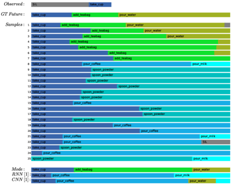
Figure 3: Qualitative result from the Breakfast dataset. This sequence corresponds to the activity of making_tea. We observe $20\%$ of the video and predict the following $50\%$. Both the generated samples and the mode of the predicted distribution are shown. The samples are ranked based on the frame-wise accuracy of the predicted activities. We also show the results of the RNN and CNN models from [1].

4.2 Anticipation without Ground-Truth Observations

Observation %	20%				30%
Prediction %	10%	20%	30%	50%	10%	20%	30%	50%
Breakfast
Baseline	0.1539	0.1365	0.1293	0.1190	0.1931	0.1656	0.1576	0.1390
Ours	0.1569	0.1400	0.1330	0.1295	0.1914	0.1718	0.1738	0.1498
50Salads
Baseline	0.2141	0.1636	0.1329	0.0939	0.2459	0.1560	0.1173	0.0857
Ours	0.2356	0.1948	0.1801	0.1278	0.2804	0.1795	0.1477	0.1206

Table 3: Results for anticipation without ground-truth observations. Numbers represent mean over classes (MoC) metric averaged over $25$ samples.

Observation %	20%				30%
Prediction %	10%	20%	30%	50%	10%	20%	30%	50%
Breakfast
Baseline	0.1655	0.1474	0.1385	0.1319	0.2080	0.1767	0.1700	0.1578
Ours	0.1671	0.1540	0.1447	0.1420	0.2073	0.1827	0.1842	0.1686
50Salads
Baseline	0.2174	0.1743	0.1496	0.1034	0.2806	0.1870	0.1460	0.0975
Ours	0.2486	0.2237	0.1988	0.1282	0.2910	0.2050	0.1528	0.1231

Table 4: Results for anticipation without ground-truth observations. Numbers represent mean over classes (MoC) metric of the predicted distribution mode.

In this section, we evaluate our approach without relying on the ground-truth annotations of the observed part. I.e. we infer the labels of the observed part of the video with the RNN-HMM model [18], and then use our approach to predict the future activities. Table 3 reports the results of the generated samples, represented by the mean over classes averaged over $25$ samples. Whereas Table 4 shows the results of the distribution mode. Our approach outperforms the baseline in both cases, which emphasizes the robustness of our approach to noisy input. Nevertheless, the baseline performs slightly better than our approach for the case of observing $30\%$ and predicting the next $10\%$ of the videos on the Breakfast dataset. This case corresponds to a short-term prediction where in most cases the future activities consist of only one action segment. Whereas our approach is better for longer time horizons.

4.3 Effect of the Number of Samples

To evaluate the generated samples, we report the mean over classes averaged over $25$ samples. Table 5 shows the effect of using different numbers of samples. In each case, the average and standard deviation of $5$ runs are reported. As shown in Table 5, the impact of the number of samples is small. While the average MoC remains in the same range, the standard deviation decreases as increasing the number of samples.

Observation %	20%				30%
Prediction %	10%	20%	30%	50%	10%	20%	30%	50%
Breakfast
5 samples	0.1547 $\pm$ 0.0014	0.1402 $\pm$ 0.0007	0.1349 $\pm$ 0.0020	0.1310 $\pm$ 0.0018	0.1907 $\pm$ 0.0017	0.1703 $\pm$ 0.0016	0.1738 $\pm$ 0.0036	0.1508 $\pm$ 0.0020
10 samples	0.1557 $\pm$ 0.0010	0.1407 $\pm$ 0.0012	0.1347 $\pm$ 0.0017	0.1302 $\pm$ 0.0013	0.1897 $\pm$ 0.0015	0.1708 $\pm$ 0.0012	0.1707 $\pm$ 0.0010	0.1502 $\pm$ 0.0010
25 samples	0.1557 $\pm$ 0.0007	0.1406 $\pm$ 0.0008	0.1342 $\pm$ 0.0007	0.1310 $\pm$ 0.0006	0.1904 $\pm$ 0.0006	0.1712 $\pm$ 0.0008	0.1718 $\pm$ 0.0011	0.1509 $\pm$ 0.0006
50 samples	0.1556 $\pm$ 0.0011	0.1400 $\pm$ 0.0006	0.1348 $\pm$ 0.0006	0.1298 $\pm$ 0.0003	0.1906 $\pm$ 0.0011	0.1712 $\pm$ 0.0005	0.1722 $\pm$ 0.0003	0.1507 $\pm$ 0.0006
50Salads
5 samples	0.2404 $\pm$ 0.0200	0.2002 $\pm$ 0.0071	0.1693 $\pm$ 0.0077	0.1247 $\pm$ 0.0078	0.2639 $\pm$ 0.0108	0.1798 $\pm$ 0.0139	0.1453 $\pm$ 0.0118	0.1199 $\pm$ 0.0044
10 samples	0.2304 $\pm$ 0.0118	0.2037 $\pm$ 0.0045	0.1739 $\pm$ 0.0054	0.1264 $\pm$ 0.0054	0.2699 $\pm$ 0.0080	0.1807 $\pm$ 0.0075	0.1468 $\pm$ 0.0095	0.1259 $\pm$ 0.0040
25 samples	0.2316 $\pm$ 0.0068	0.2003 $\pm$ 0.0040	0.1730 $\pm$ 0.0048	0.1271 $\pm$ 0.0013	0.2658 $\pm$ 0.0042	0.1822 $\pm$ 0.0062	0.1483 $\pm$ 0.0060	0.1220 $\pm$ 0.0029
50 samples	0.2308 $\pm$ 0.0032	0.1998 $\pm$ 0.0010	0.1754 $\pm$ 0.0014	0.1278 $\pm$ 0.0013	0.2664 $\pm$ 0.0030	0.1826 $\pm$ 0.0036	0.1459 $\pm$ 0.0028	0.1225 $\pm$ 0.0037

Table 5: Effect of the number of samples. Numbers represent mean over classes (MoC) metric averaged over the samples. In each case, the average and standard deviation of $5$ runs are reported.

4.4 Comparison with the State-of-the-Art

Observation %	20%				30%
Prediction %	10%	20%	30%	50%	10%	20%	30%	50%
Breakfast
RNN model [1]	0.6035	0.5044	0.4528	0.4042	0.6145	0.5025	0.4490	0.4175
CNN model [1]	0.5797	0.4912	0.4403	0.3926	0.6032	0.5014	0.4518	0.4051
Time-Cond. [8]	0.6446	0.5627	0.5015	0.4399	0.6595	0.5594	0.4914	0.4423
Ours (Mode)	0.5300	0.4410	0.3972	0.3490	0.5399	0.4453	0.4021	0.3558
Ours (Top-1)	0.7884	0.7284	0.6629	0.6345	0.8200	0.7283	0.6913	0.6239
50Salads
RNN model [1]	0.4230	0.3119	0.2522	0.1682	0.4419	0.2951	0.1996	0.1038
CNN model [1]	0.3608	0.2762	0.2143	0.1548	0.3736	0.2478	0.2078	0.1405
Time-Cond. [8]	0.4512	0.3323	0.2759	0.1727	0.4640	0.3480	0.2524	0.1384
Ours (Mode)	0.3810	0.3010	0.2633	0.1651	0.4000	0.2927	0.2317	0.1548
Ours (Top-1)	0.7489	0.5875	0.4607	0.3571	0.6739	0.5237	0.4673	0.3664

Table 6: Comparison with the state-of-the-art using ground-truth observations. Numbers represent mean over classes (MoC).

Observation %	20%				30%
Prediction %	10%	20%	30%	50%	10%	20%	30%	50%
Breakfast
RNN model [1]	0.1811	0.1720	0.1594	0.1581	0.2164	0.2002	0.1973	0.1921
CNN model [1]	0.1790	0.1635	0.1537	0.1454	0.2244	0.2012	0.1969	0.1876
Time-Cond. [8]	0.1841	0.1721	0.1642	0.1584	0.2275	0.2044	0.1964	0.1975
Ours (Mode)	0.1671	0.1540	0.1447	0.1420	0.2073	0.1827	0.1842	0.1686
Ours (Top-1)	0.2889	0.2843	0.2761	0.2804	0.3238	0.3160	0.3283	0.3079
50Salads
RNN model [1]	0.3006	0.2543	0.1874	0.1349	0.3077	0.1719	0.1479	0.0977
CNN model [1]	0.2124	0.1903	0.1598	0.0987	0.2914	0.2014	0.1746	0.1086
Time-Cond. [8]	0.3251	0.2761	0.2126	0.1599	0.3512	0.2705	0.2205	0.1559
Ours (Mode)	0.2486	0.2237	0.1988	0.1282	0.2910	0.2050	0.1528	0.1231
Ours (Top-1)	0.5353	0.4299	0.4050	0.3370	0.5643	0.4282	0.3580	0.3022

Table 7: Comparison with the state-of-the-art without ground-truth observations. Numbers represent mean over classes (MoC).

Model	Accuracy
APP-VAE [15]	62.2
Ours	57.8

Table 8: Comparison with [15]: Accuracy of predicting the label of the next action segment.

In this section, we compare our approach with the state-of-the-art methods for anticipating activities. Since the state-of-the-art methods do not model uncertainty and predict just a single sequence of future activities, we report the accuracy of the mode of the predicted distribution of our approach. Table 6 shows the results with the ground-truth observations, and Table 7 shows the results without the ground-truth observations. While the mode of the distribution from our approach only outperforms the CNN model [1] on the 50Salads dataset, it shows a lower accuracy compared to the RNN model and [8]. This is expected since these approaches were trained to predict only a single sequence of future activities while our approach is trained to predict multiple sequences. We therefore also report the top-1 MoC. The results show that our model captures the future activities better.

We also compare our approach with [15] in predicting the next action segment given all the previous segments. The accuracy of predicting the label of the future action segment is reported in Table 8. Note that in this comparison we use the ground-truth annotations of the videos as in [15]. Our approach achieves a lower accuracy. However, our approach is designed for long-term prediction as we have already observed in Section 4.2 and this comparison considers short-term prediction only. Moreover, the approach of [15] is very expensive, making it infeasible for long-term predictions.

5 Conclusion

We presented a framework for modelling the uncertainty of future activities. Both an action model and a length model are trained to predict a probability distribution over the future action segments. At test time, we used the predicted distribution to generate many samples. Our framework is able to generate a diverse set of samples that correspond to the different plausible future activities. While our approach achieves comparable results for short-term prediction, our approach is in particular useful for long-term prediction since for such scenarios the uncertainty in the future activities increases.

Acknowledgements:

The work has been funded by the Deutsche Forschungsgemeinschaft (DFG, German Research Foundation) – GA 1927/4-1 (FOR 2535 Anticipating Human Behavior) and the ERC Starting Grant ARCA (677650).

References

- [1] Yazan Abu Farha, Alexander Richard, and Juergen Gall. When will you do what?-Anticipating temporal occurrences of activities. In IEEE Conference on Computer Vision and Pattern Recognition (CVPR), pages 5343–5352, 2018.
- [2] Apratim Bhattacharyya, Mario Fritz, and Bernt Schiele. Bayesian prediction of future street scenes using synthetic likelihoods. In International Conference on Learning Representations (ICLR), 2019.
- [3] Antonino Furnari, Sebastiano Battiato, and Giovanni Maria Farinella. Leveraging uncertainty to rethink loss functions and evaluation measures for egocentric action anticipation. In European Conference on Computer Vision Workshops, pages 389–405. Springer, 2018.
- [4] Jiyang Gao, Zhenheng Yang, and Ram Nevatia. RED: Reinforced encoder-decoder networks for action anticipation. In British Machine Vision Conference (BMVC), 2017.
- [5] Farnoosh Heidarivincheh, Majid Mirmehdi, and Dima Damen. Action completion: A temporal model for moment detection. In British Machine Vision Conference (BMVC), 2018.
- [6] Minh Hoai and Fernando De la Torre. Max-margin early event detectors. International Journal of Computer Vision, 107(2):191–202, 2014.
- [7] Ashesh Jain, Amir R. Zamir, Silvio Savarese, and Ashutosh Saxena. Structural-RNN: Deep learning on spatio-temporal graphs. In IEEE Conference on Computer Vision and Pattern Recognition (CVPR), 2016.
- [8] Qiuhong Ke, Mario Fritz, and Bernt Schiele. Time-conditioned action anticipation in one shot. In IEEE Conference on Computer Vision and Pattern Recognition (CVPR), 2019.
- [9] Diederik P Kingma and Jimmy Ba. Adam: A method for stochastic optimization. In International Conference on Learning Representations (ICLR), 2015.
- [10] Hema S Koppula and Ashutosh Saxena. Anticipating human activities using object affordances for reactive robotic response. IEEE Transactions on Pattern Analysis and Machine Intelligence, 38(1):14–29, 2016.
- [11] Hilde Kuehne, Ali Arslan, and Thomas Serre. The language of actions: Recovering the syntax and semantics of goal-directed human activities. In IEEE Conference on Computer Vision and Pattern Recognition (CVPR), pages 780–787, 2014.
- [12] Tian Lan, Tsung-Chuan Chen, and Silvio Savarese. A hierarchical representation for future action prediction. In European Conference on Computer Vision (ECCV), pages 689–704. Springer, 2014.
- [13] Shugao Ma, Leonid Sigal, and Stan Sclaroff. Learning activity progression in LSTMs for activity detection and early detection. In IEEE Conference on Computer Vision and Pattern Recognition (CVPR), pages 1942–1950, 2016.
- [14] Tahmida Mahmud, Mahmudul Hasan, and Amit K Roy-Chowdhury. Joint prediction of activity labels and starting times in untrimmed videos. In IEEE International Conference on Computer Vision (ICCV), pages 5773–5782, 2017.
- [15] Nazanin Mehrasa, Akash Abdu Jyothi, Thibaut Durand, Jiawei He, Leonid Sigal, and Greg Mori. A variational auto-encoder model for stochastic point processes. In IEEE Conference on Computer Vision and Pattern Recognition (CVPR), 2019.
- [16] Antoine Miech, Ivan Laptev, Josef Sivic, Heng Wang, Lorenzo Torresani, and Du Tran. Leveraging the present to anticipate the future in videos. In IEEE Conference on Computer Vision and Pattern Recognition Workshops, 2019.
- [17] Adam Paszke, Sam Gross, Soumith Chintala, Gregory Chanan, Edward Yang, Zachary DeVito, Zeming Lin, Alban Desmaison, Luca Antiga, and Adam Lerer. Automatic differentiation in pytorch. In Advances in Neural Information Processing Systems Workshops, 2017.
- [18] Alexander Richard, Hilde Kuehne, and Juergen Gall. Weakly supervised action learning with RNN based fine-to-coarse modeling. In IEEE Conference on Computer Vision and Pattern Recognition (CVPR), 2017.
- [19] Cristian Rodriguez, Basura Fernando, and Hongdong Li. Action anticipation by predicting future dynamic images. In European Conference on Computer Vision Workshops, pages 89–105. Springer, 2018.
- [20] Michael S Ryoo. Human activity prediction: Early recognition of ongoing activities from streaming videos. In IEEE International Conference on Computer Vision (ICCV), pages 1036–1043, 2011.
- [21] Mohammad Sadegh Aliakbarian, Fatemeh Sadat Saleh, Mathieu Salzmann, Basura Fernando, Lars Petersson, and Lars Andersson. Encouraging LSTMs to anticipate actions very early. In IEEE International Conference on Computer Vision (ICCV), 2017.
- [22] Yuge Shi, Basura Fernando, and Richard Hartley. Action anticipation with RBF kernelized feature mapping RNN. In European Conference on Computer Vision (ECCV), pages 301–317, 2018.
- [23] Sebastian Stein and Stephen J McKenna. Combining embedded accelerometers with computer vision for recognizing food preparation activities. In ACM International Joint Conference on Pervasive and Ubiquitous Computing, pages 729–738, 2013.
- [24] Carl Vondrick, Hamed Pirsiavash, and Antonio Torralba. Anticipating visual representations from unlabeled video. In IEEE Conference on Computer Vision and Pattern Recognition (CVPR), pages 98–106, 2016.
- [25] Kuo-Hao Zeng, William B Shen, De-An Huang, Min Sun, and Juan Carlos Niebles. Visual forecasting by imitating dynamics in natural sequences. In IEEE International Conference on Computer Vision (ICCV), pages 2999–3008, 2017.