Marginally-calibrated deep distributional regression
Abstract
Deep neural network (DNN) regression models are widely used in applications requiring state-of-the-art predictive accuracy. However, until recently there has been little work on accurate uncertainty quantification for predictions from such models. We add to this literature by outlining an approach to constructing predictive distributions that are ‘marginally calibrated’. This is where the long run average of the predictive distributions of the response variable matches the observed empirical margin. Our approach considers a DNN regression with a conditionally Gaussian prior for the final layer weights, from which an implicit copula process on the feature space is extracted. This copula process is combined with a non-parametrically estimated marginal distribution for the response. The end result is a scalable distributional DNN regression method with marginally calibrated predictions, and our work complements existing methods for probability calibration. The approach is first illustrated using two applications of dense layer feed-forward neural networks. However, our main motivating applications are in likelihood-free inference, where distributional deep regression is used to estimate marginal posterior distributions. In two complex ecological time series examples we employ the implicit copulas of convolutional networks, and show that marginal calibration results in improved uncertainty quantification. Our approach also avoids the need for manual specification of summary statistics, a requirement that is burdensome for users and typical of competing likelihood-free inference methods.
Keywords: Calibration, Copula, Deep Neural Network, Distributional Regression, Likelihood-free Inference, Uncertainty Quantification.
1 Introduction
Deep models have become very popular in applications requiring high predictive accuracy (Goodfellow et al., 2016). In addition to being flexible, they are scalable to large datasets with high-dimensional features. However, in some applications it is crucial to represent uncertainty in predictions accurately, which is something that naïve applications of deep learning models often fail to do. This has motivated recent research on extensions that are able to capture aspects of the predictive distributions beyond the mean, and on methods to calibrate the full predictive distributions accurately. Our aim in the present work is to review and add to this existing literature in the area of distributional calibration methods for deep neural network (DNN) regression.
To do so we develop a new scalable method for ‘distributional deep regression’, by which we mean a DNN regression method that provides predictions for the full distribution. The proposed method uses the implicit copula (Nelsen, 2006, p.51) of a vector of values on a response variable that arises from a DNN regression. We call this variable a ‘pseudo-response’ because it is not observed directly. The resulting copula is a highly flexible deep function of the feature vector, which we combine with a non-parametrically estimated marginal distribution for the observed response variable. The predictive distributions from the model are marginally-calibrated (where the long-run average of the predictive distributions matches the empirically observed margin) and the approach extends the marginally-calibrated regression copula models of Klein and Smith (2019) and Smith and Klein (2019) to deep models. Even though the proposed copula is of very high dimension, we show that the likelihood is easy to compute using Bayesian methods and existing neural net libraries optimized for scalability.
Importantly, all aspects of the predictive distribution—such as the mean, variance, higher order moments and tail behaviour—are learned jointly in this deep regression. To illustrate this, and other advantages of our approach, we first consider the implicit copula of a dense layer feed-forward network, and apply the resulting distributional deep regression to two popular benchmark datasets. In both cases, our approach provides substantially more accurate predictive densities, compared to those obtained from applying the feed-forward network directly to the data with, or without, probability calibration.
However, our main application of this new distributional deep regression model is in likelihood-free inference. Here, we estimate Bayesian posterior distributions for models with intractable likelihood functions. In this case, distributional regression methods can be employed to estimate the posterior density using training samples simulated from the joint model, with the parameter as the response variable and the data as feature values. After fitting the distributional regression, the approximate posterior is obtained as the predictive distribution with feature values given by the observed data. Our approach is quite general, but in likelihood-free inference applications we show that the marginal calibration property acts to improve uncertainty quantification significantly.
To illustrate the advantages of our approach in likelihood-free inference, we construct the implicit copula of a convolutional network, and apply the resulting distributional deep regression to compute inference for two complex applications in ecological time series considered in Wood (2010) and Fasiolo et al. (2016). Wood (2010) considered the use of likelihood-free inference methods based on summary statistics for inference in state space models where the likelihood may be highly irregular. He developed an approximate likelihood, called the synthetic likelihood, which is based on a Gaussian model for a vector-valued non-sufficient summary statistic, where the summary statistic mean and covariance are estimated for each parameter value by Monte Carlo simulation. Discarding some information by using a non-sufficient summary of the data can lead to a better behaved likelihood function. A recent comparison of full likelihood and synthetic likelihood inference is given in Fasiolo et al. (2016), where some typical applications in ecology and epidemiology are described. Bayesian implementations of synthetic likelihood are discussed in detail in Price et al. (2018).
There are alternative likelihood-free inference methods for time series data, most notably the approximate Bayesian computation (ABC) framework (Sisson et al., 2018). A recent discussion of ABC methods for time series is given in Frazier et al. (2019) who suggest that accurate estimation of the posterior on parameters is not always necessary for accurate forecasting. However, like synthetic likelihood and its extensions, ABC methods require suitable summary statistics for the data. Even without the requirement that these statistics be multivariate normal for every parameter value, choosing statistics that are informative and low-dimensional is difficult. A major advantage of our proposed approach is that manually specified summary statistics are not required, and instead the whole dataset is used as the feature vector in a regression model. A further comparison of our approach and alternative likelihood-free inference methods is given in Section 5.
The rest of the paper is organized as follows. Section 2 introduces deep learning regression models, and uncertainty quantification of predictions from such models. Section 3 shows how the copula smoother of Klein and Smith (2019) can be extended to the DNN case, including computation of the predictive distributions. Section 4 illustrates our approach using dense layer feed-forward networks for two benchmark datasets. Section 5 reviews likelihood-free inference, and uses an implicit copula constructed from a convolutional network to perform likelihood-free inference in two complex ecological time series models. A comparison to some leading alternative approaches is also provided, while Section 6 concludes.
2 Deep Learning for Regression
In this section we briefly introduce deep learning regression models, and review the existing literature on uncertainty quantification for deep learning.
2.1 Deep learning regression models
Suppose we observe response and feature values , , where is the scalar response and the vector of feature values. A feed-forward neural network specifies a function of the input features through a sequence of transformations called ‘layers’. The feature vector, , enters the model at an initial input layer, while the final transformation gives the predicted response at an output layer; the intermediate component transformations are the hidden layers. The inputs to any layer come from previous layers. For an introduction to neural network terminology from a statistical perspective see overviews by Polson and Sokolov (2017) and Fan et al. (2019).
In this paper we consider DNNs for regression with a single response. A DNN can be written as a function , where is the set of all parameters (weights) in the network. We assume that the activation function for the output layer is linear, so that
| (1) |
where are the output layer coefficients, are the coefficients of all other layers (so that ), and is the vector of basis functions defined by the last hidden layer of the network. In general an intercept is also included, although in Section 3 we set in the output layer because implicit copulas are location free.555Note that in Section 3 the random variable is a pseudo-response, and we construct the implicit copula of its data distribution.
Training of a neural network such as (1) is usually done by minimizing a penalized empirical loss function with respect to . A popular loss in regression problems is the squared error over the observed values of the response, given by
| (2) |
A regularization penalty—such as the or norm of the weights—is often used to prevent over-fitting and simplify the optimization. Regularization can also be undertaken in an implicit manner in the optimization algorithm, using a variety of methods such as early stopping, drop-out or batch normalization; see Goodfellow et al. (2016) for an introduction to these ideas. For posterior mode estimation in a Bayesian framework, the loss is equivalent to the negative log-likelihood and an explicit penalty is equivalent to the negative log prior density. When (2) is used in a regression setting, it is equivalent to assuming a homoscedastic Gaussian model, although minimization of (2) can be justified on grounds which do not require parametric model assumptions. Thus, the simplest way to construct predictive distributions for future responses is to use a Gaussian predictive density, after estimating the response variance. However, in many applications more sophisticated uncertainty quantification is necessary, which is the focus of the current paper.
In our approach we consider an initial DNN regression fit, from which data-dependent basis functions are obtained. These basis functions are constructed using optimized standard neural network libraries, which are then employed in our Bayesian copula regression model outlined in Section 3.
Our methodology is related to that of Nalenz and Villani (2018), where data-dependent basis functions from tree ensemble methods were further used within a Bayesian statistical model with shrinkage priors to obtain uncertainty quantification. It is also related to a ‘neural linear model’ (Ober and Rasmussen, 2019), where a statistical linear model is used for the output layer of a DNN regression, because we consider a Bayesian neural linear model for a pseudo-response in Section 3.2.
2.2 Uncertainty quantification for deep learning
Gneiting et al. (2007) discuss different ways to gauge the accuracy of uncertainty quantification in prediction, and we focus on two of these: ‘probability calibration’ and ‘marginal calibration’. Gneiting et al. (2007) define notions of calibration formally by considering a sequence of forecasting problems indexed by time. “Nature” chooses a distribution at time , from which an outcome is drawn, and the forecaster gives a predictive distribution . Intuitively, probability calibration means that an event predicted to have probability occurs with relative frequency , formalized by the requirement that
Roughly speaking, marginal calibration is where the average of nature’s true distribution should match the average forecast distribution, so that
if the limits on the left- and right-hand sides above exist. In practice, while is unknown, a draw from it is observed and can be replaced with a point mass at this value, so that is the empirical distribution function.
In the current work, the forecaster is a regression model and is its predictive distribution. We do not follow the above theoretical framework strictly in our later development. For example, our regression is applied to cross-sectional data, so that time ordering does not apply. However, as noted in Gneiting et al. (2007), the above framework can still provide related empirical notions of marginal calibration. Gneiting and Ranjan (2013) develop such a notion by considering the forecast distribution as a random measure, and there is a joint distribution of this random measure and the observation. Marginal calibration can be defined as equality of the marginal distribution of the observation and the expected forecast distribution.
Discussions of uncertainty quantification often make a distinction between aleatoric and epistemic uncertainty. Aleatoric uncertainties are those which cannot be reduced in principle, whereas epistemic uncertainties arise from knowledge that it is possible to possess, but is not available. Examples of epistemic uncertainty in statistical modelling are model uncertainty and parameter uncertainty. The distinction between aleatoric and epistemic uncertainty is important in some applications of deep learning models, such as extrapolating predictions to regions of the feature space not covered by the training set (Kendall and Gal, 2017).
In the deep learning literature previous approaches to achieving accurate uncertainty quantification are of two main types, which we discuss separately below.
2.2.1 Post-processing calibration adjustments
The first approach uses post-processing adjustments to achieve probability calibration. The early machine learning literature on this topic is concerned with classification problems (e.g. Platt (2000)), while calibration in regression has received far less attention in the machine learning literature. One approach for regression is due to Keren et al. (2018), who consider discretizing a continuous response so that calibration methods developed for classifiers can be applied. A related method is described in Li et al. (2019), who consider classification methods which account for the ordering of a finely discretized response.
Another approach, which we compare to our own later, is due to Kuleshov et al. (2018) and can be briefly explained as follows. Suppose we have a training set of features and responses, and a regression model has been fitted to them. The fitted model provides predictive distributions for the response for any value of the feature vector. Now consider a calibration set of features and responses, which may be disjoint from the training set. For every probability we can ask what is the value such that the -quantiles of the predictive distributions upper bound a relative frequency of of the responses in the calibration set? We then adjust all predictive distributions such that the -quantile is changed to the corresponding -quantile. This adjustment can be achieved using isotonic regression for a set of and pairs, and is a form of probability calibration.
Our method described in Section 3 ensures that the marginal distribution of the model response matches an empirical estimate. However, whether the ergodic averaging of predictive distributions leads to equality with the model marginal distribution depends on the properties of the regression copula. However, we show that the average predictive distribution from our method reproduces the empirically estimated marginal well in the examples.
Kuleshov et al. (2018), in their discussion of the notion of marginal calibration in Gneiting et al. (2007), state that “We found that their notion of marginal calibration was too weak for our purposes, since it only preserves guarantees relative to the average distribution.” In contrast, we show that marginal calibration can be highly constraining at times, so that it complements probability calibration post-processing. In our experience, it is particularly effective when the response distribution is skewed, heavy-tailed or bounded.
2.2.2 Distributional regression approaches
A second approach to uncertainty quantification for deep learning models in regression is to use more flexible models that can capture apects of the response distribution beyond the mean. For example, loss functions equivalent to Gaussian log-likelihoods with heteroscedasticity have been considered by Kendall and Gal (2017) and Lakshminarayanan et al. (2017), among others, where both the mean and log-variance are flexible functions of the features. However, with such an approach the response distribution is still conditionally Gaussian, which will result in a lack of calibration in some problems. These authors also consider various other innovations designed to improve uncertainty quantification, including uncertainties relating to feature vectors which are unusual compared to the training set. A deep version of quantile regression has been recently considered by Tagasovska and Lopez-Paz (2018) as a method for modelling the whole distribution, but enforcing monotonicity in the estimated quantiles is difficult. Rodrigues and Pereira (2018) consider a deep multi-task quantile learning approach which can help to avoid the crossing quantiles problem. Mixture density networks and their extensions are another neural approach to distributional regression possessing a universal approximation property (Bishop, 1994; Uria et al., 2013). Tran et al. (2019) consider using deep learning predictors within generalized linear and mixed models, as do Hubin et al. (2018) who also focus on the difficult problem of accounting for model uncertainty in the architecture and suggesting Markov chain Monte Carlo (MCMC) algorithms for computation.
Beyond neural network methods, there are a wide variety of methods for distributional regression in the statistical and machine learning literatures. Approaches include Bayesian non-parametric methods (Foti and Williamson, 2015) and the generalized additive models for location, scale and shape framework of Rigby and Stasinopoulos (2005). The latter authors suggest using parametric response distributions beyond the exponential family, and model the mean, scale and shape parameters as functions of the covariates; see also Mayr et al. (2012); Klein et al. (2015) and Umlauf et al. (2018). A problem with many existing distributional regression methods is that they do not scale well to large datasets, and computationally cheaper distributional regression methods are necessary in some applications.
Bayesian methods for training neural networks are also motivated by the need for improved uncertainty quantification. Bayesian predictive distributions, where parameter and possibly model uncertainty is integrated out according to the posterior distribution, is a convenient way to account for these epistemic uncertainties in prediction. Recent work in this direction includes Blundell et al. (2015); Hernandez-Lobato and Adams (2015); Gal and Ghahramani (2016); Khan et al. (2018); Kingma et al. (2015) and Teye et al. (2018) among others, while MacKay (1992) and Neal (1996) were pioneers of Bayesian neural networks. A recent review of deep learning methods emphasizing the connections between existing algorithms and models and Bayesian inference is given by Polson and Sokolov (2017).
3 Marginally-Calibrated Deep Learning Regression
Klein and Smith (2019) and Smith and Klein (2019) introduce a new approach to distributional regression that uses a copula decomposition to ensure marginal calibration. We outline how to extend their approach to deep learning regression.
3.1 Copula model
Consider realizations of a continuous-valued response, with corresponding feature values . Following Sklar (1959), the joint density of the distribution can always be written as
| (3) |
with . Here, is a -dimensional copula density with , and is the distribution function of ; both of which are typically unknown. Smith and Klein (2019) call such a copula a ‘regression copula’666This should not be confused with the term ‘copula regression’ which is sometimes used to refer to a low-dimensional copula model for a multivariate response with regression margins. because it is a function of the features . In copula modelling it is common to replace in (3) with the density of a parametric copula with parameters , and we do so here with , which is the implicit copula of a DNN regression specified below in Section 3.2. Klein and Smith (2019) suggest calibrating the distribution of to its invariant margin, so that density with distribution function estimated non-parametrically. Thus, the copula model is
| (4) |
We stress that even though is assumed invariant with respect to , the response is still affected by the features though the joint distribution, which Smith and Klein (2019) point out has two consequences. First, the entire marginal predictive distribution of a future response given in Section 3.4 is a function of the feature vector . Second, the implicit copula developed below has some additional latent parameters , and the marginal distribution that also conditions on is also a function of , analogous to the specification of a standard regression model.
3.2 Regression copula
The key to the success of our approach is the specification of the regression copula with density . For this we employ the implicit copula of a pseudo-response vector from a DNN regression model derived as follows. Consider a pseudo-response given by the output layer observed with Gaussian noise, so that if is distributed independently ,
| (5) |
Then from (1), the vector of realizations is given by the linear model
| (6) |
with an matrix. The regression (6) does not contain an intercept, since an intercept term is not identified in the copula. We assume that is known so that the basis functions are fixed, and the procedure for obtaining is described later. To produce smooth and efficient estimates we regularize the basis coefficient vectors . In a Bayesian context this corresponds to adopting a shrinkage prior, with a common choice being the conditionally Gaussian prior
where is a sparse precision matrix that is a function of regularization parameters .
We extract the copula of the distribution of the pseudo-response vector with integrated out. Such a copula is either called an ‘implicit’ (McNeil et al., 2005, p.190) or ‘inversion’ (Nelsen, 2006, p.51) copula because it is constructed by inverting Sklar’s theorem. The copula is -dimensional with a dependence structure that is a function of the feature values . To derive this copula, first notice that under the linear model and Gaussian prior
which is derived in Section 2.1 of Klein and Smith (2019). The implicit copula of this distribution is called the Gaussian copula, and it is constructed by standardizing the distribution above to have zero mean and unit variances. To do so here, we set , where is a diagonal scaling matrix with elements , which ensures that . The resulting Gaussian copula has density
| (7) |
where
| (8) |
, , and and are the densities of and distributions, respectively.
Because does not feature in the expression for , it is therefore unidentified, so that we simply set it equal to 1 throughout the rest of the paper.777We stress that this does not mean the observed response has unit variance, but instead has a marginal variance given by . This is because implicit copulas are always invariant to the scale of the pseudo-response. Also, while the copula is -dimensional—and therefore potentially of very high dimension—the matrix at (8) is a parsimonious function of . Klein and Smith (2019) give expressions for for three different shrinkage priors, and we consider two different choices here:
Horseshoe:
The horseshoe prior is attractive due to its robustness, local adaptivity and analytical properties (Carvalho and Polson, 2010). It is a scale mixture, where , with prior and . With this prior , with , and .
Ridge:
The ridge prior is one of the simplest forms of shrinkage priors, where and we use the scale-dependent prior of Klein and Kneib (2016) for . With this prior , while .
To link the two regression copulas in (3) and (4), it is straightforward to see that for some prior density . Klein and Smith (2019) highlight that even though is a Gaussian copula, is not, although computation of through integration with respect to has to be undertaken numerically. Last, the horseshoe prior has a larger copula parameter vector , so that is likely to have a richer dependence structure. Because the horseshoe is a ‘global-local’ shrinkage prior, this is likely to allow for a more accurate dependence structure when is large and sparse as with our DNN basis functions, as we show in our later empirical work.
3.3 Estimation
We employ a multi-stage estimator with the following three steps:
Algorithm 1 (Estimation of Distributional Deep Regression)
-
1.
Estimate the marginal using a non-parametric estimator, for which we use the kernel density estimator of Shimazaki and Shinomoto (2010).
-
2.
Given , compute pseudo-response values , for . Using existing neural net libraries applied to , construct output layer basis functions , and evaluate them at the feature values to obtain .
-
3.
Given and , compute the augmented posterior distribution using MCMC, where the margin is therefore the posterior of the copula parameters.
Step 2 is dependent upon the choice of architecture, which we discuss later in the context of each application. Step 3 is the main challenge, where computing the posterior requires evaluation of the likelihood, which is given by the copula decomposition at (4). To do so directly requires evaluation of the copula density at (7), which is computationally infeasible in general because of the need to invert the matrix . Klein and Smith (2019) solve this problem by instead using the likelihood conditional also on , which is
and can be evaluated in operations because is diagonal. These authors propose standard MCMC schemes that generate and , so that is integrated out in a Monte Carlo manner and direct computation of is avoided. We refer readers to Klein and Smith (2019) for further details on these samplers, which produce J Monte Carlo draws from the augmented posterior distribution .
3.4 Predictive densities
The predictive density of a new observation of the response , given new feature values , is estimated using its Bayesian posterior predictive density
Klein and Smith (2019) propose an estimator for the above that is fast to compute, based on the Monte Carlo draws from Step 3 of Algorithm 1. It is given by
| (9) |
where , , and . Full derivation is given in the Web Appendix.
The density forecast (9) is a direct function of the feature vector and is readily computed at any point in the feature space. It is a Gaussian density for transformed using the nonlinear transformation that does not depend on the features. Nevertheless, because and are highly nonlinear functions of the features via the DNN representation, the entire density—not just the location and scale—is a flexible function of . It is worth stressing that our approach does not have the universal approximation property of some alternative distributional regression approaches. However, the semi-parametric nature of the method allows it to be both computationally efficient, and effective with small training datasets, as we demonstrate empirically in the examples below.
4 Dense Feed-Forward Network Examples
To illustrate our approach we construct a regression copula from a dense layer deep feed-forward network, and apply it to two widely used benchmark regression datasets.
Description of datasets
The first dataset is the Boston housing data (Harrison and Rubinfeld, 1978) with observations and 14 features, while the second is the Framingham cholesterol data (Zhang and Davidian, 2001) with observations and 202 features.888The first dataset is available from the UCI machine learning repository, http://archive.ics.uci.edu/ml/machine-learning-databases/housing/, while the second was taken from the qrLMM package in R. The latter is longitudinal data, where extra dummy variables were included to account for different individuals. Both feature sets include binary, categorical and continuous variables, the latter of which we standardize to the unit interval.
DNN architecture
We considered our DNN copula (labelled ‘DNNC’) with both ridge and horseshoe regularization priors. For the feed-forward network we used ReLU activation functions for one to three hidden layers, along with a linear activation function for the output layer. At Step 2 of Algorithm 1, we obtained the basis functions of the linear activation layer using the package keras in R (Chollet and Allaire, 2018). We found that two hidden layers of size 64 without additional L2 regularization are sufficient and use them combined with a dropout rate of 0.5. In training the network early stopping was used based on ten-fold cross-validation in both cases, with the optimization run for 200 epochs and batch size equal to the sample size. The optimizer used is adam with default settings from keras, see the Web Appendix for details.
Benchmarks
The predictions from the DNNC are compared to four benchmarks. The first is a feed-forward network with the same architecture above, but applied directly to the response data with disturbances and non-zero intercept for the output layer (labelled ‘DNN’). We combine this with a ridge prior for . The second benchmark is a recalibration of the predictive densities from the DNN obtained using the approach of Kuleshov et al. (2018) (labelled ‘DNN-recalibrated’). The third benchmark is a mixture density network implemented in the R-package CaDENCE (Cannon, 2012) (labelled ‘MDN’). We choose a two-component Gaussian mixture with all distribution parameters (the means, standard deviations and mixing weight) to be learned through a 2-hidden layer FNN.
Measuring accuracy
To judge accuracy of the predictive distributions, they are evaluated at the observed feature values to give predictive densities using (9), from which distribution functions are also computed. From these we constructed the following three measures of accuracy.
-
(i)
The first is a plot of the average predictive density
overlaid on a histogram of the response values. We use this plot to assess marginal calibration of the different methods.
-
(ii)
The second is a plot to assess probability calibration. Consider an increasing set of values , and define
to be the relative frequency of observations falling below the -quantile of the predictive distribution, where denotes the cardinality of a set. If a method produces probability calibrated predictive distributions then . In our later examples we plot versus , with deviations from zero in the former indicating a lack of calibration.
-
(iii)
The third is the mean in- and out-of-sample logarithmic score. To compute the latter we use ten-fold cross-validation as follows. Partition the data into ten approximately equally-sized sub-samples of sizes , denoted here as for . For each observation in sub-sample we compute the predictive density using the remaining nine sub-samples as the training data, and denote these densities here as . The ten-fold mean out-of-sample logarithmic score is then
Empirical results
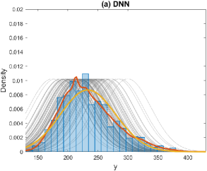
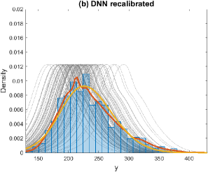
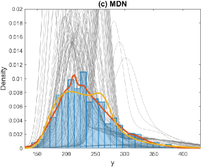
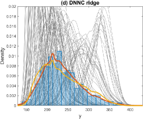
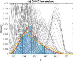
To first illustrate the difference in methods, Figures 1 and 2 plot the predictive densities , evaluated at observations in the Boston housing and cholesterol datasets, respectively. For visual clarity, we only plot densities for observations that correspond to the first 100 ordered response values in the data sets, resulting in 100 predictive densities. Each panel corresponds to a different method, and also includes a histogram of the response values and an adaptive kernel density estimate (KDE). In panel (a) the DNN produces homoscedastic Gaussian densities, whereas in panel (b) the DNN-recalibrated method produces densities that are non-Gaussian, but still homoscedastic. In contrast, the DNNC provides non-parametric predictions in panels (d) and (e) which are highly heteroscedastic. As discussed in depth in Smith and Klein (2019), a key strength of the regression copula modelling approach is that the entire predictive distribution—including higher order moments—can vary with feature values. The MDN method in panel (c) produces predictive densities that are similar to the DNNC methods.
Figures 3 and 4 show both calibration plots for the different methods and two datasets. We make four observations. First, the DNN is neither marginally nor probability calibrated. Second, the DNN-recalibrated is probability calibrated well by construction, but this does not lead to marginal calibration, which can be very poor, such as in Figure 3(b). Third, in contrast, the DNNC—whether using either the horseshoe or ridge prior for regularization—exhibits accurate marginal calibration, along with near probability calibration. Fourth, the MDN method exhibits good probability calibration and better marginal calibration than DNN and DNN-recalibrated, although not as good as the DNNC methods.
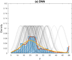
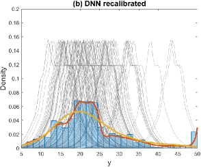
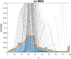
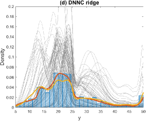
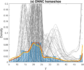
Results are given for (a) DNN, (b) DNN-recalibrated, (c) MDN, (d) DNNC-ridge, and (e) DNNC-horseshoe. Each panel depicts predictive densities (grey lines) for 100 of the observations, corresponding to first 100 observations of the ordered response values. Also shown are a histogram (blue) and KDE (red line) of the response, and the average predictive density (yellow). Accurate marginal calibration is indicated by the red and yellow lines being very close.
Results are given for (a) DNN, (b) DNN-recalibrated, (c) MDN, (d) DNNC-ridge, and (e) DNNC-horseshoe. Each panel depicts predictive densities (grey lines) for 100 of the observations, corresponding to the first 100 observations of the ordered response values. Also shown are a histogram (blue) and KDE (red line) of the response, and the average predictive density (yellow). Accurate marginal calibration is indicated by the red and yellow lines being very close.
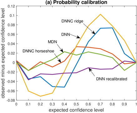
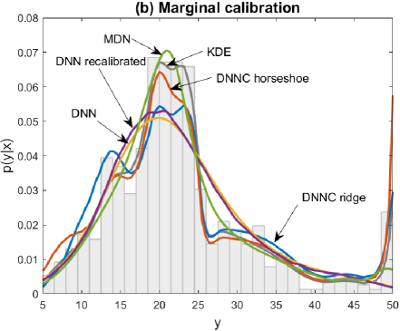
Panel (a) gives the probability calibration plot (with the y-axis showing difference between the observed and expected confidence levels to enhance visibility), and panel (b) the marginal calibration plot. Results are provided for the DNN (yellow line), DNN-recalibrated (violet line), MDN (green line) DNNC-ridge (blue line), DNNC-horseshoe (red line). Also shown in (b) is the kernel density estimate (grey line) and a histogram (grey) of the response.
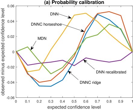
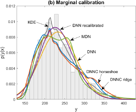
Panel (a) gives the probability calibration plot (with the y-axis showing difference between the observed and expected confidence levels to enhance visibility), and panel (b) the marginal calibration plot. Results are provided for the DNN (yellow line), DNN-recalibrated (violet line), MDN (green line) DNNC-ridge (blue line), DNNC-horseshoe (red line). Also shown in (b) is the kernel density estimate (grey line) and a histogram (grey) of the response.
Finally, Table 1 reports the in- and out-of-sample mean logarithmic scores for the two datasets, and we make three observations. First, the DNN performs poorly, which is because the response distributions are non-Gaussian in both examples. Second, the shrinkage prior considered for matters, with the predictions using the horseshoe prior superior to those using the ridge prior in both examples. Last, the DNNC is clearly more accurate than the benchmarks DNN and DNN-recalibrated, and slightly more than MDN. MDNs have a universal approximation property which may be important in some problems.
| Data | DNN | DNN- | MDN | DNNC- | DNNC- |
| recal. | ridge | horseshoe | |||
| In-sample log-scores | |||||
| Boston | -2.69(0.060) | -2.62(0.056) | -2.39(0.049) | -2.39(0.041) | -2.17(0.041) |
| Chol. | -5.08(0.027) | -4.22(0.030) | -4.65(0.034) | -4.35(0.026) | -4.31(0.026) |
| Predictive log-scores | |||||
| Boston | -2.84(0.084) | -2.61(0.047) | -2.61(0.065) | -2.71(0.056) | -2.56(0.056) |
| Chol. | -5.14(0.030) | -5.09(0.029) | -5.19(0.047) | -5.05(0.030) | -5.07(0.032) |
Scores for each of the five methods are given in the columns, and for both in-sample (top half) and out-of-sample (bottom half) predictions. The latter are constructed using ten-fold cross-validation, as discussed in the text. Higher values correspond to more accurate predictive densities, with the highest values for each case in bold. Standard errors for the means are also given in parentheses.
5 Application to Likelihood-Free Inference
In this section we discuss likelihood-free inference. We will discuss here only regression approaches to likelihood-free inference. For a recent comprehensive overview of alternative methods see Sisson et al. (2018). We show how to use the distributional deep regression copula model in Section 3 to perform likelihood-free inference, and highlight the advantage of marginal calibration—which is an intrinsic aspect of the copula model—in this context. To illustrate, a regression copula is constructed from a convolutional network, and the resulting copula model is used to construct likelihood-free inference in two empirical applications. Convolutional networks are used in situations where the features take the form of a time series or an image, and the layers of the network can be thought of as extracting local characteristics of the input and then combining these into increasingly abstract representations. See Polson and Sokolov (2017) and Fan et al. (2019) for further background.
5.1 Likelihood-free inference
5.1.1 Introduction
Let denote the parameters in a parametric statistical model for data observed from a sampling distribution with density . Consider Bayesian inference with prior density , and observed data denoted as , so that the posterior density is .999We denote the data vector as , rather than , to avoid confusion with the response values from the distributional deep regression copula model outlined in Section 3. Suppose we can simulate data , as , . We refer to the density as the ‘joint model’ for the data and parameters. By definition, the posterior density is the conditional density of given obtained from this joint density. In cases where the likelihood function is intractable (but the model can still be simulated from), we can use a regression fitted to the simulated data to approximate the conditional density of given in the joint model. Fitting a regression model to data , , where is the response and is the feature vector, will give a predictive density for any . The predictive density is then an approximation to the posterior density based on the regression model. Thus, selecting a regression method that produces an accurate density estimate is key to conducting accurate likelihood-free inference in this approach.
Later we consider only modelling scalar functions of using separate regressions, rather than a multivariate regression model. Posterior distributions for one-dimensional functions of the parameter are enough for scientific inferences in many cases, although the joint posterior is needed for some purposes. Predictive inference requires the full joint posterior, and even for scientific inferences a joint posterior on several parameters may sometimes be required. For example, Wood (2010) considers the assessment of different dynamic regimes for the blowfly data discussed in Section 5.2, which are dependent on several of the model parameters. Multivariate extensions of our methods are left to future work.
5.1.2 Advantage of marginal calibration
For simplicity, we denote scalar functions of as . Then the marginal distribution for the regression training data , is the prior . In this case, marginal calibration as defined in Section 2.2 occurs when the marginal distribution for (i.e. here) matches the average posterior predictive density from the regression model. Moreover, this average is a sample-based estimate of , because the values are simulated from density . Therefore, if the marginal calibration property holds for the regression method then we have
| (10) |
To highlight why it is advantageous for such a property to hold, write the joint Bayesian model as and then notice that
| (11) |
which shows that marginal calibration always holds for the true posterior density. Thus it is desirable for the regression-based approximations to the posterior to respect this kind of calibration also. However, while marginal calibration is a necessary quality for a regression approximation of the posterior to be good, it is not sufficient. For example, if we always estimate the posterior density by the prior regardless of the data, then this approximation method is marginally calibrated but does not give good posterior approximations. Nevertheless, we show empirically in our later examples that our copula method achieves both better marginal calibration and uncertainty quantification than benchmark methods.
5.1.3 Previous flexible regression models for likelihood-free inference
The use of flexible regression models for conditional density estimation in likelihood-free inference is not new. For example, Fan et al. (2013) consider flexible regression models for approximating the summary statistic distribution, and hence the likelihood, based on a copula of a mixture and flexible mixture of experts regression estimates of summary statistic marginal distributions. Raynal et al. (2018) consider applying the quantile regression forests method of Meinshausen (2006) to likelihood-free inference. Izbicki and Lee (2017) describe methods for converting high-dimensional regression methods into flexible conditional density estimators using orthogonal series estimators, and Izbicki et al. (2019) consider initial estimates obtained from an ABC sampler, and then applying non-parametric conditional density estimators which make use of a surrogate loss function to estimate the conditional density locally. Papamakarios and Murray (2016) consider a neural network approach using a sequential decomposition of the posterior into conditional distributions and mixture density network models for the conditionals. They also consider the use of a sequential design strategy to concentrate more on the high posterior probability region of the parameter space. Further improvements on this methodology are given in Lueckmann et al. (2017). Papamakarios et al. (2019) consider autoregressive flows to learn approximations to the likelihood, avoiding the difficulties of removing the bias arising from the use of a proposal in the sequential design step in Papamakarios and Murray (2016) and Lueckmann et al. (2017). However, methods such as those of Papamakarios et al. (2019) and Fan et al. (2013) require use of a conventional Bayesian computational algorithm for summarizing the posterior once the approximate likelihood has been obtained. Heteroscedastic neural network methods have also been used in post-processing adjustments of conventional ABC samplers (Blum and François, 2010), where empirical residuals are used within the fitted regression model to give particle approximations to the posterior. The method of Blum and François (2010) builds on the earlier seminal paper of Beaumont et al. (2002).
Many of the regression methods discussed above require the use of summary statistics for their application. In contrast, our approach does not require summary statistics, and makes use of convolutional neural networks (CNNs) for specifying the marginal posterior distributions, where the time series values are used directly as features of the CNNs in our copula-based distributional regression model. Jiang et al. (2017) is the first work, of which we are aware, that uses deep learning methods to automate the choice of summary statistics in likelihood-free inference, although they do not consider convolutional networks. Convolutional networks have been used in likelihood-free inference for time series by Dinev and Gutmann (2018), where similar to Jiang et al. (2017) the regression is being used as an automated way of obtaining summary statistics, rather than for density estimation in itself. Greenberg et al. (2019) suggest a way to use a proposal which focuses on a relevant part of the parameter space without the difficulties of the proposal corrections in Papamakarios and Murray (2016) and Lueckmann et al. (2017), and also avoiding additional computations after the conditional density estimation step. In their method, a parametrized family of approximations is considered, such as Gaussian or a mixture of Gaussians, and a mapping from the data to the parameters in the approximation is learned using a certain loss function. In the case of time series data, it may be possible to avoid the use of summary statistics using this approach for a suitable neural network parametrization of the function mapping the data to the parameters of the approximation. The general principle of marginal calibration can be applied in conjunction with some of the other flexible regression methods for specification of the all aspects of the posterior distribution described above, complementing the existing literature on flexible regression methods in likelihood-free inference.
5.2 Convolutional network examples
In the context of likelihood-free inference for time series models, Dinev and Gutmann (2018) considered using a CNN regression model to predict the components of the parameter vector based on data , using a training set of simulations of pairs which are generated from the joint model. Dinev and Gutmann (2018) consider multivariate outputs to predict all parameters jointly and use the predictions of the network as an automated summary statistic choice. Here we will use the DNN regression copula model in Section 3 as a distributional regression method to directly estimate the marginal posterior distributions of the elements of .
We show the potential of our proposed approach (labelled DNNC) in two complex ecological time series examples. In both examples we simulate 10000 data sets under the prior, and use 8000 data sets for training and 2000 for testing, denoted as and , respectively. Each simulated series has the same length as the observed data. In the simulation, the accuracy of parameter predictions can be measured directly for different likelihood-free methods. For the real data, we can split the data and measure the accuracy of the parameter point estimates using a composite scoring rule for the different methods.
Although the whole time series is used as the feature vector in our regression models, our methodology scales well with . CNNs can be trained easily even for long series using standard deep learning libraries. Additionally, because of the way CNNs extract local information from the series (by applying filters with fixed weights, and then combining this information at different scales), the number of weights to be learned does not grow rapidly with for suitable network architectures.
Nicholson’s blowfly model
As the first example we consider the data reported by Nicholson (1954) from laboratory experiment E2 to elucidate the population dynamics of sheep blowfly (Lucilia cuprina). Wood (2010) modelled the observed dynamics of the population at time as , where
is the delayed recruitment process with parameters , , , , and
is the adult survival process. Here, , are independent gamma disturbances with unit mean and variances and , respectively. Consequently, , and the length of the series is . We use the prior for specified in Table 13 of Fasiolo et al. (2016) and given in the Web Appendix.
A chaotic prey-predator model for modelling voles abundance
The second model we consider is used by Fasilio and Wood (2018) to describe the dynamics of Fennoscandian voles (Microtus and Clethrionomys). There has been an observed shift in voles abundance dynamics from low-amplitude oscillations in central Europe and southern Fennoscandia to high-amplitude fluctuations in the north. One possible reason is the absence of generalist predators in the north, where voles are hunted primarily by weasels (Mustela nivalis). In the notation of Fasilio and Wood (2018), the predator-prey dynamics are given by the following system of differential equations (Turchin and Ellner, 2000)
where , , is a Brownian motion process with constant volatility ; and and represent voles and weasels abundances, respectively. Turchin and Ellner (2000) considered a mechanistic version of this model without the driving Brownian motion, and investigate the effects of environmental noise through perturbing the model parameters. The model is formulated in continuous time, with the parameters and representing intrinsic population growth rates of voles and weasels respectively, while is the carrying capacity of . Averaging of these parameters is done over the seasonal component with amplitude and period equal to one year. Peak growth is achieved in summer. Further, and as well as and are the parameters of type II and III functional response models of generalist predation and predation by weasels, respectively; see Fasilio and Wood (2018) for further details. These authors assume the number of trapped voles to be Poisson distributed, , at times when trapping took place. Finally, the model is not fitted directly to data but rescaled to a dimensionless form, where
and
In this dimensionless form of the model we continue to write for the Brownian motion scale parameter, although it is not the same parameter in the two models. We used the same strategy as Fasilio and Wood (2018) to arrive at data points collected during the spring (mid-June) and autumn (September) of each year between 1952 and 1997. The priors on the parameter are specified in the Web Appendix.
CNN architecture
To set up the basis functions for our DNNC in Step 2 of Algorithm 1, we fitted separate CNNs for each model parameter (six parameters for the blowfly model, nine for the voles abundance model) with pseudo-responses as outputs and the simulated series as features. Beginning with the generic architecture suggested in Dinev and Gutmann (2018) and experimenting also with other specifications, we ended up using two convolutional layers with 31/7 filters, and kernel sizes of 31/10 for the blowfly and voles examples respectively. In the later cross-validation comparisons where training based on the first 80% of the series is considered, the kernel sizes were 31/8 for the blowfly and voles data, respectively. We used ReLU activation functions for the convolutional layers with L2 regularization with parameter 0.001, followed by two dense layers of sizes 100/1 and ReLU/linear activation functions for the first and second dense layers respectively. It is important to not normalize the inputs as this may destroy the time series structure. Instead we use batch normalization after each layer. The number of epochs was determined by cross-validation and a batch-size of 256. As before we employed the optimizer adam with default settings. As proposed by Dinev and Gutmann (2018) we apply a max-pooling layer after the first convolutional layer and a flattening layer after the second one. Extracting the resulting basis functions was done as in the previous subsection using the keras package.
Benchmark models
To compare our DNNC method with, we consider the following benchmark methods, with methods (iii) to (vi) being leading approaches in likelihood-free inference:
-
(i)
DNN:uses the same CNN architecture as employed to construct the copula, but applied directly to the original response values, and with Gaussian errors in the output layer.
-
(ii)
DNNCss: uses summary statistics as features in the regression and the copula methodology of Section 4 with a two hidden layer FNN.
- (iii)
-
(iv)
ABCrf: ABC with random forests, as implemented in the R package abcrf by Marin et al. (2017).
-
(v)
BSL: the Bayesian synthetic likelihood approach implemented in the R package BSL by An et al. (2019)).
-
(vi)
semiBSL: a semi-parametric version of BSL which estimates a Gaussian copula model with non-parametric marginal distributions, as implemented in the R package BSL.
The methods DNNCss, BSL, semiBSL, ABC and ABCrf require summary statistics, and we used the same choices as Fasiolo et al. (2016) and Fasilio and Wood (2018) (23 statistics for the blowfly data and 16 for the voles data) and implemented in the R packages synlik (Fasiolo and Wood, 2018) and volesModel (available on Github). Most of these methods require careful implementation, and we give extensive details on these in Appendix A, and additional comments on the computational demands of each approach in the Web Appendix. Due to the high computational cost we exclude BSL and semiBSL from the simulation but use them for the two real data analyses.
| ABC | ABCrf | DNN | DNNC | DNNCss | |
|---|---|---|---|---|---|
| 1.35 (0.046/0.50) | 1.30 (0.047/0.48) | 1.21 (0.043/0.62) | 1.02 (0.037/0.75) | 1.32 (0.043/0.66) | |
| 0.48 (0.014/0.82) | 0.50 (0.015/0.77) | 0.41 (0.010/0.87) | 0.33 (0.013/0.89) | 0.46 (0.014/0.88) | |
| 1.38 (0.054/0.54) | 1.41 (0.056/0.44) | 1.33 (0.035/0.77) | 0.80 (0.050/0.95) | 1.35 (0.052/0.77) | |
| 1.44 (0.063/0.74) | 1.54 (0.064/0.67) | 1.05 (0.050/0.90) | 0.96 (0.051/0.94) | 1.41 (0.059/0.85) | |
| 0.29 (0.018/0.70) | 0.31 (0.021/0.66) | 0.20 (0.016/0.92) | 0.21 (0.016/0.96) | 0.27 (0.017/0.88) | |
| 1.11 (0.049/0.87) | 1.14 (0.050/0.86) | 0.92 (0.043/0.95) | 0.88 (0.041/0.95) | 1.07 (0.046/0.90) |
Each cell gives the mean squared error for the logarithm of the parameters, along with its standard error and coverage of the 95% credible interval in parentheses. Each row corresponds to a different parameter, while the columns give results for the ABC, ABCrf, DNN, DNNC and DNNCss methods.
| ABC | ABCrf | DNN | DNNC | DNNCss | |
|---|---|---|---|---|---|
| 0.04 (0.002/0.94) | 0.02 (0.001/0.99) | 0.03 (0.001/0.92) | 0.03 (0.001/0.94) | 0.03 (0.001/0.97) | |
| 0.81 (0.046/0.95) | 0.16 (0.010/0.99) | 0.24 (0.014/0.93) | 0.19 (0.017/0.94) | 0.34 (0.024/0.97) | |
| 1.56 (0.069/0.95) | 1.36 (0.060/0.97) | 1.23 (0.053/0.94) | 1.17 (0.057/0.95) | 1.36 (0.060/0.95) | |
| 0.27 (0.009/0.95) | 0.25 (0.008/0.96) | 0.23 (0.008/0.94) | 0.22 (0.008/0.95) | 0.23 (0.001/0.95) | |
| 0.92 (0.065/0.95) | 0.39 (0.025/0.99) | 0.39 (0.031/0.93) | 0.36 (0.037/0.95) | 0.47 (0.042/0.97) | |
| 0.60 (0.023/0.95) | 0.32 (0.013/0.98) | 0.33 (0.014/0.92) | 0.32 (0.014/0.94) | 0.36 (0.015/0.96) | |
| 0.59 (0.032/0.94) | 0.19 (0.014/0.98) | 0.19 (0.018/0.94) | 0.17 (0.022/0.95) | 0.18 (0.027/0.96) | |
| 0.72 (0.030/0.94) | 0.21 (0.006/0.99) | 0.30 (0.016/0.96) | 0.26 (0.015/0.93) | 0.23 (0.013/0.96) | |
| 0.32 (0.073/0.95) | 0.36 (0.016/0.99) | 0.41 (0.034/0.97) | 0.34 (0.037/0.95) | 0.35 (0.034/0.96) |
Each cell gives the mean squared error for the logarithm of the parameters, along with its standard error and coverage of the 95% credible interval in parentheses. Each row corresponds to a different parameter, while the columns give results for the ABC, ABCrf, DNN, DNNC and DNNCss methods.
Measures of performance
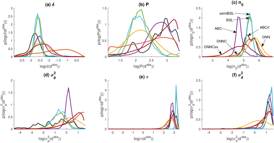
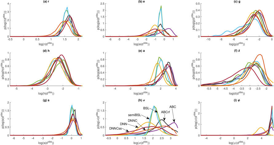
Tables 2 and 3 report mean squared errors, standard errors and coverage rates of 95% credible intervals (in parentheses the latter two) for the logarithm of the parameters in the simulated test data sets for both applications. Figures 5 and 6 depict the average marginal posteriors of the log-parameters averaging over the 2,000 test replicates, to examine marginal calibration of different methods.
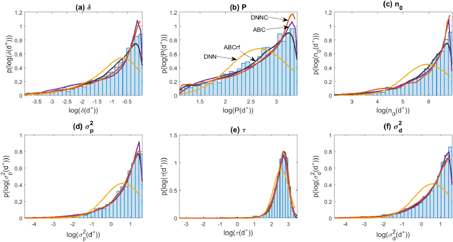
Panels (a) to (f) show the average marginal predictive densities for the four methods ABC (violet line), ABCrf (gray line), DNN (yellow line), DNNC (red line). Also shown in blue is a histogram of the simulated test data.
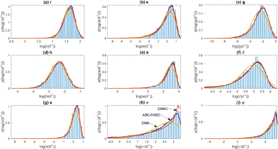
Panels (a) to (f) show the average marginal predictive densities for the four methods ABC (violet line), ABCrf (gray line), DNN (yellow line), DNNC (red line). Also shown in blue is a histogram of the simulated test data.
Shown are the marginal posteriors (averages) of log-parameters for the observed blowfly data (80% of the series) for the six methods: BSL (green line), semiBSL (blue line), ABC (purple line), ABCrf (gray line), DNN (yellow line), DNNC (red line), DNNCss (dark red line).
Shown are the marginal posteriors (averages) of log-parameters for the observed blowfly data (80% of the series) for the six methods: BSL (green line), semiBSL (blue line), ABC (purple line), ABCrf (gray line), DNN (yellow line), DNNC (red line), DNNCss (dark red line).
Comparison of the performance of different methods when applied to the observed data, is undertaken using data splitting. Here, the first 80% of the time series is used as training data, while the last 20% is test data used to assess out-of-sample predictive performance. Joint posterior predictive inference is not considered, because our own method as well as the ABCrf approach estimates only marginal posterior distributions. Figures 7 and 8 show the estimated marginal posterior densities of the parameters for all competing methods. The figures show that inferences can differ substantially between different methods for some of the parameters, particularly for the blowfly data. To examine whether the different fits are reasonable, our predictive comparison of the different methods using data splitting uses a composite scoring rule (Dawid and Musio, 2014) based on plug-in predictive densities using posterior mean point estimates for different methods. Consider a sequence of pairwise marginal predictive distributions , with being the posterior mean parameters and consecutive time points in the test part of the series. With point estimates obtained from training data , and test data consisting of , out of sample predictive performance is measured by the composite logarithmic score (CLS) and composite energy score (CES) defined as
where is the multivariate energy score for the pair (Gneiting et al., 2008). The multivariate energy score is the natural generalization of the continuous ranked probability score to a multivariate setting. The composite scores CLS and CES are easier to compute than alternative scoring rules that involve looking at a full joint distribution for . The bivariate predictive densities are estimated using kernel estimates based on Monte Carlo simulation from the model. We report the scores (with standard errors) in Table 4, where we compute the negative values so that higher values are better.
| Score | BSL | semiBSL | ABC | ABCrf | DNN | DNNC | DNNCss |
| Blowfly Data | |||||||
| Log. Score | -16.49 | -16.52 | -16.89 | -16.65 | -16.88 | -16.78 | -17.05 |
| Neg. Energy | -1934.34 | -1936.63 | -2380.18 | -1826.64 | -1979.15 | -1956.89 | -2245.12 |
| Voles Data | |||||||
| Log. Score | -11.09 | -11.17 | -10.46 | -10.90 | -14.56 | -10.48 | -12.36 |
| Neg. Energy | -48.62 | -49.54 | -42.62 | -44.05 | -61.13 | -37.65 | -58.17 |
The columns show the composite scores for the six methods for both data sets (top: Blowfly; bottom: Voles). Higher values correspond to more accurate predictive results with the highest values for each case in bold.
Results
We make five observations on the simulations. First, our DNNC outperforms all benchmark models, with smallest simulation MSE values, and with coverage rates closest to the nominal 95% level. ABCrf was also a strong performer for the voles data, although with slightly conservative uncertainty assessments. Second, DNNC performs better than DNNCss, so that the use of the convolutional network rather than user-selected summary statistics makes a difference to the performance of our method. Third, ABC, DNNC and ABCrf calibrate well marginally, while DNN is poorly calibrated in general. Fourth, simulation MSE values and coverage rates for the ABC and ABCrf are very similar for the blowfly example. Finally, in the comparison of different methods based on the composite scoring rules, DNNC is fourth best for the blowfly data and the best for the voles data for the composite energy score. For the composite logarithmic score, DNNC is fourth best for the blowfly data and second best for the voles data.
6 Discussion
In this work we have contributed to the growing literature on uncertainty quantification for deep neural network regression models, exploring a marginal calibration approach using the implicit copula of a deep neural network. Our approach is complementary to existing post-processing adjustments of neural network regression approaches which attempt to achieve probability calibration. We have focused particularly on applications to likelihood-free inference for times series models using convolutional networks to avoid the need for hand-crafted summary statistics. For these applications the marginal calibration property has a strong motivation as imposing a consistency requirement on regression approximations to the posterior density that holds for the true posterior density.
We have only been concerned in this work with regressions for a scalar response. In the case of our motivating likelihood-free applications, often posterior densities for scalar functions of the parameter are all that are required for scientific inferences, but the joint posterior may be required for some interpretive purposes as well as full posterior predictive inference. It would be possible to extend the approach considered here to a multivariate response. There are at least three ways this could be done. First, by incorporating some of the simulated parameter values into the features in the regression, it would be possible to estimate full conditional posterior densities for individual parameters. Then these estimated full conditionals could be used in a likelihood-free Gibbs sampling scheme (Clarté et al., 2019; Rodrigues et al., 2020). A related approach involves ordering the parameters, considering a corresponding sequential decomposition of the posterior distribution, and then estimating the univariate conditional distributions in the decomposition using regression. A third approach would describe the dependence between components of the response using a copula. It would also be interesting in future work to apply the marginal calibration principle to other regression-based likelihood-free approximations that have been suggested in the literature.
Acknowledgments
The authors would like to thank the Associate Editor and two Referees for inspiring comments that helped to improve upon the first version of this paper. Nadja Klein acknowledges
support through the Emmy Noether grant KL 3037/1-1 of the German research
foundation (DFG). David Nott was supported by a Singapore Ministry of Education
Academic Research Fund Tier 1 grant (R-155-000-189-114). We thank Matteo Fasiolo for sharing his experience on the prior choices, the data and simulators for both likelihood-free data examples.
Appendix A
This appendix gives some additional details on the implementation of some of the benchmark methods employed in Section 5.
-
DNNCss: In the FNN, each hidden layer was of size 64, with ReLU/linear activations and dropout rate of 0.5.
-
ABC: We found that using the maximal possible size of 30 for the number of nodes in the hidden layer of the DNN worked best. The regularization parameter for the weights in the neural network was chosen by cross-validation, and with a tolerance of one that corresponds to no rejection step in the ABC procedure, which is recommended for high-dimensional settings. Bounded parameters were transformed to the real line using logistic transformations.
-
ABCrf: For tuning the ABCrf method, we used trees and tuned several other algorithmic parameters (mtry, the number of randomly chosen features to consider for splits in the trees, sample.fraction the sample fraction of points used in constructing the trees and min.node.size, the node size at which splitting stops) using the tuneRanger package (Probst et al., 2018); see the Web Appendix for the optimal hyper-parameter settings obtained. Raynal et al. (2018) emphasize increasing training sample size to control variability and monitoring out-of-bag error. However, in a simulation study it is not possible to adaptively increase the training sample size based on one of the methods. The default random forests implementation gives poor results with the sample size used here, with overfitting evident in both examples, but after tuning with the tuneRanger package performance was greatly improved.
-
BSL and semiBSL: Both are run with steps and a diagonal covariance for the proposal until convergence. We then take the covariance of these samples as a proposal for the final run.
Both the BSL and semiBSL can experience numerical difficulties if the MCMC starting value is in the posterior tail, so we initialized these using the posterior mean parameters of ABC.
References
- (1)
- An et al. (2019) An, Z., South, L. F. and Drovandi, C. C. (2019). BSL: Bayesian Synthetic Likelihood. R package version 2.0.0.
- Beaumont et al. (2002) Beaumont, M. A., Zhang, W. and Balding, D. J. (2002). Approximate Bayesian computation in population genetics, Genetics 162: 2025–2035.
- Bishop (1994) Bishop, C. (1994). Mixture density networks, Technical Report NCRG/4288, Aston University, Birmingham, UK.
- Blum and François (2010) Blum, M. G. B. and François, O. (2010). Non-linear regression models for approximate Bayesian computation, Statistics and Computing 20: 63–75.
- Blundell et al. (2015) Blundell, C., Cornebise, J., Kavukcuoglu, K. and Wierstra, D. (2015). Weight uncertainty in neural network, in F. Bach and D. Blei (eds), Proceedings of the 32nd International Conference on Machine Learning, Vol. 37 of Proceedings of Machine Learning Research, PMLR, Lille, France, pp. 1613–1622.
- Cannon (2012) Cannon, A. J. (2012). Neural networks for probabilistic environmental prediction: Conditional density estimation network creation and evaluation (cadence) in r, Computers and Geosciences 41: 126–135.
- Carvalho and Polson (2010) Carvalho, C. M. and Polson, Nicholas, G. (2010). The horseshoe estimator for sparse signals, Biometrika 97: 465–480.
- Chollet and Allaire (2018) Chollet, F. and Allaire, J. J. (2018). Deep Learning with R, 1st edn, Manning Publications Co., Greenwich, CT, USA.
- Clarté et al. (2019) Clarté, G., Robert, C. P., Ryder, R. and Stoehr, J. (2019). Component-wise approximate Bayesian computation via Gibbs-like steps, arXiv preprint arXiv:1905.13599 .
- Csilléry et al. (2012) Csilléry, K., François, O. and Blum, M. G. B. (2012). ABC: an R package for approximate Bayesian computation (ABC), Methods in Ecology and Evolution 3: 475–479.
- Dawid and Musio (2014) Dawid, A. P. and Musio, M. (2014). Theory and applications of proper scoring rules, METRON 72(2): 169–183.
- Dinev and Gutmann (2018) Dinev, T. and Gutmann, M. (2018). Dynamic likelihood-free inference via ratio estimation (DIRE), arXiv:1810.09899 .
- Fan et al. (2019) Fan, J., Ma, C. and Zhong, Y. (2019). A selective overview of deep learning, arXiv preprint arXiv:1904.05526 .
- Fan et al. (2013) Fan, Y., Nott, D. J. and Sisson, S. A. (2013). Approximate Bayesian computation via regression density estimation, Stat 2(1): 34–48.
- Fasilio and Wood (2018) Fasilio, M. and Wood, S. (2018). ABC in ecological modelling, in S. A. Sisson, Y. Fan and M. Beaumont (eds), Handbook of Approximate Bayesian Computation, Chapman & Hall, CRC, Boca Raton, pp. 597–623.
- Fasiolo et al. (2016) Fasiolo, M., Pya, N. and Wood, S. N. (2016). A comparison of inferential methods for highly nonlinear state space models in ecology and epidemiology, Statistical Science 31(1): 96–118.
- Fasiolo and Wood (2018) Fasiolo, M. and Wood, S. (2018). An introduction to synlik (2014). R package version 0.1.2.
- Foti and Williamson (2015) Foti, N. J. and Williamson, S. A. (2015). A survey of non-exchangeable priors for Bayesian nonparametric models, IEEE Transactions on Pattern Analysis and Machine Intelligence 37(2): 359–371.
- Frazier et al. (2019) Frazier, D. T., Maneesoonthorn, W., Martin, G. M. and McCabe, B. P. (2019). Approximate Bayesian forecasting, International Journal of Forecasting 35(2): 521–539.
- Gal and Ghahramani (2016) Gal, Y. and Ghahramani, Z. (2016). Dropout as a Bayesian approximation: Representing model uncertainty in deep learning, in M. F. Balcan and K. Q. Weinberger (eds), Proceedings of The 33rd International Conference on Machine Learning, Vol. 48 of Proceedings of Machine Learning Research, PMLR, New York, New York, USA, pp. 1050–1059.
- Gneiting et al. (2007) Gneiting, T., Balabdaoui, F. and Raftery, A. E. (2007). Probabilistic forecasts, calibration and sharpness, Journal of the Royal Statistical Society Series B 69(2): 243–268.
- Gneiting and Ranjan (2013) Gneiting, T. and Ranjan, R. (2013). Combining predictive distributions, Electronic Journal of Statistics 7: 1747–1782.
- Gneiting et al. (2008) Gneiting, T., Stanberry, L. I., Grimit, E. P., Held, L. and Johnson, N. A. (2008). Assessing probabilistic forecasts of multivariate quantities, with an application to ensemble predictions of surface winds, TEST 17(2): 211–235.
- Goodfellow et al. (2016) Goodfellow, I., Bengio, Y. and Courville, A. (2016). Deep Learning, MIT Press. http://www.deeplearningbook.org.
- Greenberg et al. (2019) Greenberg, D. S., Nonnenmacher, M. and Macke, J. H. (2019). Automatic posterior transformation for likelihood-free inference, https://arxiv.org/abs/1905.07488 .
- Harrison and Rubinfeld (1978) Harrison, D. and Rubinfeld, D. L. (1978). Hedonic prices and the demand for clean air, Journal of Environmental Economics and Management 5: 81–102.
- Hernandez-Lobato and Adams (2015) Hernandez-Lobato, J. M. and Adams, R. (2015). Probabilistic backpropagation for scalable learning of Bayesian neural networks, in F. Bach and D. Blei (eds), Proceedings of the 32nd International Conference on Machine Learning, Vol. 37 of Proceedings of Machine Learning Research, PMLR, Lille, France, pp. 1861–1869.
- Hubin et al. (2018) Hubin, A., Storvik, G. and Frommlet, F. (2018). Deep Bayesian regression models, arXiv preprint arXiv:1806.02160 .
- Izbicki and Lee (2017) Izbicki, R. and Lee, A. B. (2017). Converting high-dimensional regression to high-dimensional conditional density estimation, Electronic Journal of Statistics 11: 2800–2831.
- Izbicki et al. (2019) Izbicki, R., Lee, A. B. and Pospisil, T. (2019). ABC–CDE: Toward approximate Bayesian computation with complex high-dimensional data and limited simulations, Journal of Computational and Graphical Statistics (To appear).
- Jiang et al. (2017) Jiang, B., Wu, T.-y., Zheng, C. and Wong, W. H. (2017). Learning summary statistic for approximate bayesian computation via deep neural network, Statistica Sinica pp. 1595–1618.
- Kendall and Gal (2017) Kendall, A. and Gal, Y. (2017). What uncertainties do we need in Bayesian deep learning for computer vision?, Advances in Neural Information Processing Systems 30: Annual Conference on NeurIPS, Long Beach, CA, USA, pp. 5580–5590.
- Keren et al. (2018) Keren, G., Cummins, N. and Schuller, B. (2018). Calibrated prediction intervals for neural network regressors, arXiv preprint arXiv:1803.09546 .
- Khan et al. (2018) Khan, M., Nielsen, D., Tangkaratt, V., Lin, W., Gal, Y. and Srivastava, A. (2018). Fast and scalable Bayesian deep learning by weight-perturbation in Adam, in J. Dy and A. Krause (eds), Proceedings of the 35th International Conference on Machine Learning, ICML 2018, Stockholmsmässan, Stockholm, Sweden, July 10-15, 2018, Vol. 80 of Proceedings of Machine Learning Research, PMLR, pp. 2611–2620.
- Kingma et al. (2015) Kingma, D. P., Salimans, T. and Welling, M. (2015). Variational dropout and the local reparameterization trick, in C. Cortes, N. D. Lawrence, D. D. Lee, M. Sugiyama and R. Garnett (eds), Advances in Neural Information Processing Systems 28, Curran Associates, Inc., pp. 2575–2583.
- Klein and Kneib (2016) Klein, N. and Kneib, T. (2016). Scale-dependent priors for variance parameters in structured additive distributional regression, Bayesian Analysis 11(4): 1071–1106.
- Klein et al. (2015) Klein, N., Kneib, T. and Lang, S. (2015). Bayesian generalized additive models for location, scale, and shape for zero-inflated and overdispersed count data, Journal of the American Statistical Association 110(509): 405–419.
- Klein and Smith (2019) Klein, N. and Smith, M. S. (2019). Implicit copulas from Bayesian regularized regression smoothers, Bayesian Analysis 14(24): 1143–1171.
- Kuleshov et al. (2018) Kuleshov, V., Fenner, N. and Ermon, S. (2018). Accurate uncertainties for deep learning using calibrated regression, Proceedings of the 35th International Conference on Machine Learning, ICML 2018, Stockholmsmässan, Stockholm, Sweden, July 10-15, 2018, pp. 2801–2809.
- Lakshminarayanan et al. (2017) Lakshminarayanan, B., Pritzel, A. and Blundell, C. (2017). Simple and scalable predictive uncertainty estimation using deep ensembles, in I. Guyon, U. V. Luxburg, S. Bengio, H. Wallach, R. Fergus, S. Vishwanathan and R. Garnett (eds), Advances in Neural Information Processing Systems 30, Curran Associates, Inc., pp. 6402–6413.
- Li et al. (2019) Li, R., Bondell, H. D. and Reich, B. J. (2019). Deep distribution regression, https://arxiv.org/abs/1903.06023 .
- Lueckmann et al. (2017) Lueckmann, J.-M., Goncalves, P. J., Bassetto, G., Öcal, K., Nonnenmacher, M. and Macke, J. H. (2017). Flexible statistical inference for mechanistic models of neural dynamics, in I. Guyon, U. V. Luxburg, S. Bengio, H. Wallach, R. Fergus, S. Vishwanathan and R. Garnett (eds), Advances in Neural Information Processing Systems 30, Curran Associates, Inc., pp. 1289–1299.
- MacKay (1992) MacKay, D. J. C. (1992). A practical Bayesian framework for backpropagation networks, Neural Computation 4(3): 448–472.
- Marin et al. (2017) Marin, J.-M., Raynal, L., Pudlo, P., Robert, C. and Estoup, A. (2017). abcrf: approximate Bayesian computation via random forests. R package version 1.7.
- Mayr et al. (2012) Mayr, A., Fenske, N., Hofner, B., Kneib, T. and Schmid, M. (2012). Generalized additive models for location, scale and shape for high dimensional data—a flexible approach based on boosting, Journal of the Royal Statistical Society: Series C (Applied Statistics) 61(3): 403–427.
- McNeil et al. (2005) McNeil, A. J., Frey, R. and Embrechts, R. (2005). Quantitative Risk Management: Concepts, Techniques and Tools, Princeton University Pres, Princton: NJ.
- Meinshausen (2006) Meinshausen, N. (2006). Quantile regression forests, J. Mach. Learn. Res. 7: 983–999.
- Nalenz and Villani (2018) Nalenz, M. and Villani, M. (2018). Tree ensembles with rule structured horseshoe regularization, The Annals of Applied Statistics 12(4): 2379–2408.
- Neal (1996) Neal, R. (1996). Bayesian Learning for Neural Networks, Lecture Notes in Statistics, Springer New York.
- Nelsen (2006) Nelsen, R. B. (2006). An Introduction to Copulas., Springer-Verlag, New York, Secaucus, NJ, USA.
- Nicholson (1954) Nicholson, A. J. (1954). An outline of the dynamics of animal populations, Australian Journal of Zoology 2: 9–65.
- Ober and Rasmussen (2019) Ober, S. W. and Rasmussen, C. E. (2019). Benchmarking the neural linear model for regression, arXiv preprint arXiv:1912.08416 .
- Papamakarios and Murray (2016) Papamakarios, G. and Murray, I. (2016). Fast -free inference of simulation models with Bayesian conditional density estimation, in D. D. Lee, M. Sugiyama, U. V. Luxburg, I. Guyon and R. Garnett (eds), Advances in Neural Information Processing Systems 29, Curran Associates, Inc., pp. 1028–1036.
- Papamakarios et al. (2019) Papamakarios, G., Sterratt, D. and Murray, I. (2019). Sequential neural likelihood: Fast likelihood-free inference with autoregressive flows, in K. Chaudhuri and M. Sugiyama (eds), Proceedings of Machine Learning Research, Vol. 89, pp. 837–848.
- Platt (2000) Platt, J. (2000). Probabilistic outputs for support vector machines and comparison to regularize likelihood methods, in A. Smola, P. Bartlett, B. Schoelkopf and D. Schuurmans (eds), Advances in Large Margin Classifiers, pp. 61–74.
- Polson and Sokolov (2017) Polson, N. G. and Sokolov, V. (2017). Deep learning: A Bayesian perspective, Bayesian Analysis 12(4): 1275–1304.
- Price et al. (2018) Price, L. F., Drovandi, C. C., Lee, A. C. and Nott, D. J. (2018). Bayesian synthetic likelihood, Journal of Computational and Graphical Statistics 27(1): 1–11.
- Probst et al. (2018) Probst, P., Wright, M. and Boulesteix, A.-L. (2018). Hyperparameters and tuning strategies for random forest, Wiley Interdisciplinary Reviews: Data Mining& Knowledge Discovery .
- Raynal et al. (2018) Raynal, L., Marin, J.-M., Pudlo, P., Ribatet, M., Robert, C. P. and Estoup, A. (2018). ABC random forests for Bayesian parameter inference, Bioinformatics 35(10): 1720–1728.
- Rigby and Stasinopoulos (2005) Rigby, R. A. and Stasinopoulos, D. M. (2005). Generalized additive models for location, scale and shape, Journal of the Royal Statistical Society Series C 54(3): 507–554.
- Rodrigues and Pereira (2018) Rodrigues, F. and Pereira, F. C. (2018). Beyond expectation: Deep joint mean and quantile regression for spatio-temporal problems, https://arxiv.org/abs/1808.08798 .
- Rodrigues et al. (2020) Rodrigues, G., Nott, D. and Sisson, S. (2020). Likelihood-free approximate Gibbs sampling, Statistics and Computing (To Appear).
- Shimazaki and Shinomoto (2010) Shimazaki, H. and Shinomoto, S. (2010). Kernel bandwidth optimization in spike rate estimation, Jorunal of Computational Neuroscience 29(1-2): 171–182.
- Sisson et al. (2018) Sisson, S. A., Fan, Y. and Beaumont, M. (2018). Handbook of Approximate Bayesian Computation, Chapman & Hall/CRC, New York.
- Sklar (1959) Sklar, A. (1959). Fonctions de repartition a n dimensions et leur marges, Publ. Inst. Statist. Univ. Paris 8, 229231 8: 229–231.
- Smith and Klein (2019) Smith, M. S. and Klein, N. (2019). Bayesian inference for regression copulas, Journal of Business and Economic Statistics (To Appear).
- Tagasovska and Lopez-Paz (2018) Tagasovska, N. and Lopez-Paz, D. (2018). Frequentist uncertainty estimates for deep learning, arXiv preprint arXiv:1811.00908 .
- Teye et al. (2018) Teye, M., Azizpour, H. and Smith, K. (2018). Bayesian uncertainty estimation for batch normalized deep networks, Proceedings of the 35th International Conference on Machine Learning, ICML 2018, Stockholmsmässan, Stockholm, Sweden, July 10-15, 2018, pp. 4914–4923.
- Tran et al. (2019) Tran, M.-N., Nguyen, N., Nott, D. and Kohn, R. (2019). Bayesian deep net GLM and GLMM, Journal of Computational and Graphical Statistics 29(1): 97–113.
- Turchin and Ellner (2000) Turchin, P. and Ellner, S. P. (2000). Living on the edge of chaos: Population dynamics of fennoscandian voles, Ecology 81(11): 3099–3116.
- Umlauf et al. (2018) Umlauf, N., Klein, N. and Zeileis, A. (2018). BAMLSS: Bayesian additive models for location, scale, and shape (and beyond), Journal of Computational and Graphical Statistics 27(3): 612–627.
- Uria et al. (2013) Uria, B., Murray, I. and Larochelle, H. (2013). RNADE: The real-valued neural autoregressive density-estimator, in C. J. C. Burges, L. Bottou, M. Welling, Z. Ghahramani and K. Q. Weinberger (eds), Advances in Neural Information Processing Systems 26, Curran Associates, Inc., pp. 2175–2183.
- Wood (2010) Wood, S. N. (2010). Statistical inference for noisy nonlinear ecological dynamic systems, Nature 466(7310): 1102–1104.
- Zhang and Davidian (2001) Zhang, D. and Davidian, M. (2001). Linear mixed models with flexible distributions of random effects for longitudinal data, Biometrics 57(3): 795–802.