An Evaluation of Feature Matchers for
Fundamental Matrix Estimation

Abstract

Matching two images while estimating their relative geometry is a key step in many computer vision applications. For decades, a well-established pipeline, consisting of SIFT, RANSAC, and 8-point algorithm, has been used for this task. Recently, many new approaches were proposed and shown to outperform previous alternatives on standard benchmarks, including the learned features, correspondence pruning algorithms, and robust estimators. However, whether it is beneficial to incorporate them into the classic pipeline is less-investigated. To this end, we are interested in i) evaluating the performance of these recent algorithms in the context of image matching and epipolar geometry estimation, and ii) leveraging them to design more practical registration systems. The experiments are conducted in four large-scale datasets using strictly defined evaluation metrics, and the promising results provide insight into which algorithms suit which scenarios. According to this, we propose three high-quality matching systems and a Coarse-to-Fine RANSAC estimator. They show remarkable performances and have potentials to a large part of computer vision tasks. To facilitate future research, the full evaluation pipeline and the proposed methods are made publicly available.

1 Introduction

Matching two images while recovering their geometric relation, e.g., epipolar geometry [Hartley and Zisserman(2003)], is one of the most basic tasks in computer vision and a crucial step in many applications such as Structure-from-Motion (SfM) [Agarwal et al.(2011)Agarwal, Furukawa, Snavely, Simon, Curless, Seitz, and Szeliski, Heinly et al.(2015)Heinly, Schonberger, Dunn, and Frahm, Radenovic et al.(2016)Radenovic, Schönberger, Ji, Frahm, Chum, and Matas, Schönberger et al.(2015)Schönberger, Radenovic, Chum, and Frahm, Schönberger and Frahm(2016)] and Visual SLAM [Mur-Artal et al.(2015)Mur-Artal, Montiel, and Tardos, Davison et al.(2007)Davison, Reid, Molton, and Stasse, Forster et al.(2014)Forster, Pizzoli, and Scaramuzza]. In these applications, the overall performance heavily depends on the quality of the initial two-view registration. Consequently, a thorough performance evaluation for this module is of vital importance to the computer vision community. However, to the best of our knowledge, no previous work has done it. To this end, we are dedicated to an extensive experimental evaluation of existing algorithms to establish a uniform evaluation protocol in this paper.

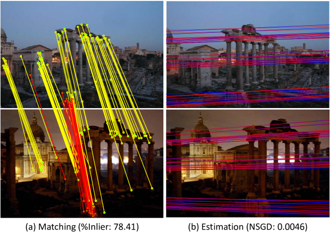
Figure 1: Outputs of the two-view matching and geometry estimation pipeline. (a) shows matching results with yellow/red lines standing for inliers/outliers. (b) shows epipolar geometry estimation results with red/blue lines standing for the ground-truth/estimated epipolar lines. We use the proposed normalized symmetric geometric distance (NSGD) to measure the estimation accuracy. The smaller, the better.

For decades, a classic pipeline has been used for this task, which relies on the SIFT [Lowe(2004)] features to establish initial correspondences across images, then prunes bad correspondences by Lowe’s ratio test [Lowe(2004)], and finally estimates the geometry using RANSAC [Fischler and Bolles(1981)] based estimators. We are here interested in recovering the fundamental matrix (FM), which suits more general scenes than other geometric models, e.g., the homography and essential matrix. Fig. 1 shows an example output of this pipeline. Here, we mainly focus on the geometry estimation quality.

Recently, many new approaches were proposed which showed potentials to this task, including the learned features [Mishchuk et al.(2017)Mishchuk, Mishkin, Radenovic, and Matas, Luo et al.(2018)Luo, Shen, Zhou, Zhu, Zhang, Yao, Fang, and Quan, Mishkin et al.(2018)Mishkin, Radenovic, and Matas], robust estimators [Raguram et al.(2013)Raguram, Chum, Pollefeys, Matas, and Frahm, Barath and Matas(2018)], and, especially, correspondence pruning algorithms [Bian et al.(2017)Bian, Lin, Matsushita, Yeung, Nguyen, and Cheng, Ma et al.(2018)Ma, Zhao, Jiang, Zhou, and Guo, Yi et al.(2018)Yi, Trulls, Ono, Lepetit, Salzmann, and Fua] which revived comparatively little attention over before. However, while these algorithms outperform earlier ones on standard benchmarks, incorporating them into the classic pipeline may not necessarily translate into a performance increase. For example, Balntas et al. [Balntas et al.(2016)Balntas, Riba, Ponsa, and Mikolajczyk] showed that descriptors which perform better than others on the standard benchmark [Brown et al.(2011)Brown, Hua, and Winder] do not show a better image matching quality. The inconsistency was also shown and discussed in [Bian et al.(2017)Bian, Lin, Matsushita, Yeung, Nguyen, and Cheng, Yi et al.(2018)Yi, Trulls, Ono, Lepetit, Salzmann, and Fua, Schönberger et al.(2017)Schönberger, Hardmeier, Sattler, and Pollefeys].

In this paper, we conduct a comprehensive evaluation of recently proposed algorithms by incorporating them into the well-established image matching and epipolar geometry estimation pipeline to investigate whether they can increase the overall performance. In detail, this paper makes the following contributions:

• i) We present an evaluation protocol for local features, robust estimators, and especially correspondence pruning algorithms such as [Bian et al.(2017)Bian, Lin, Matsushita, Yeung, Nguyen, and Cheng, Yi et al.(2018)Yi, Trulls, Ono, Lepetit, Salzmann, and Fua, Ma et al.(2018)Ma, Zhao, Jiang, Zhou, and Guo] which have not been carefully investigated.

• ii) We evaluate algorithms on four large-scale datasets using strictly defined metrics. The results provide insights into which datasets are particularly challenging and which algorithms suit which scenarios.

• iii) Based on the results, we propose three high-quality and efficient matching systems, which perform on par with the powerful CODE [Lin et al.(2017)Lin, Wang, Cheng, Yeung, Torr, Do, and Lu] system but are several orders of magnitude faster.

• iv) Interestingly, we observe that the recent GC-RANSAC [Barath and Matas(2018)] (also USAC [Raguram et al.(2013)Raguram, Chum, Pollefeys, Matas, and Frahm]) does not show consistently high performance on geometry estimation but permits effective outlier pruning. We hence propose to first use it for outlier removal, and then apply LMedS based estimator [Rousseeuw and Leroy(1987)] for model fitting. The resulting approach, termed Coarse-to-Fine RANSAC, shows significant superiority over other alternatives.

2 Related work

Rich research focuses on evaluating local features and robust estimators, while correspondence pruning algorithms have not been well evaluated. The proposed benchmark mitigates this gap.

Evaluating Local Features.

Mikolajczyk et al. [Mikolajczyk et al.(2005)Mikolajczyk, Tuytelaars, Schmid, Zisserman, Matas, Schaffalitzky, Kadir, and Van Gool] evaluated the affine region detectors on small-scale datasets, which cover various photometric and geometric image transformations. Later, Mikolajczyk and Schmid [Mikolajczyk and Schmid(2005)] extended the evaluation to local descriptors. Build upon this, Heinly et al.[Heinly et al.(2012)Heinly, Dunn, and Frahm] proposed several additional metrics and datasets to evaluate binary descriptors. Besides, Brown et al. [Brown et al.(2011)Brown, Hua, and Winder] presented a patch pair classification benchmark for the learned descriptors, which measures the ability of a descriptor to discriminate positive from negative patch pairs. Recently, Balntas et al.[Balntas et al.(2017)Balntas, Lenc, Vedaldi, and Mikolajczyk] evaluated the hand-crafted and learned descriptors in terms of the verifying and retrieving homography patches. Schönberger et al.[Schönberger et al.(2017)Schönberger, Hardmeier, Sattler, and Pollefeys] comparatively evaluated these two types of descriptors in the context of image-based reconstruction.

Evaluating Robust Estimators.

Choi et al.[Choi et al.(1997)Choi, Kim, and Yu] conducted an evaluation of RANSAC [Fischler and Bolles(1981)] family in terms of the line fitting and homography estimation [Hartley and Zisserman(2003)], where the accuracy, runtime, and robustness of methods are analyzed. Lacey et al.[Lacey et al.(2000)Lacey, Pinitkarn, and Thacker] performed an evaluation of RANSAC algorithms for stereo camera calibration. Raguram et al.[Raguram et al.(2008)Raguram, Frahm, and Pollefeys] categorized RANSAC algorithms and provide a comparative analysis on them, where the trade-off between efficiency and accuracy is considered. These protocols evaluate robust model fitting techniques in both synthetic and real data. Torr et al. [Torr and Murray(1997), Torr and Zissermann(1997)] provided performance characterization of fundamental matrix (FM) estimation algorithms. Zhang [Zhang(1998)] reviewed FM estimation techniques and proposed a well-founded measure to compute the distance of two fundamental matrices, which is shown to better than using the Frobenius norm. Armanguè et al. [Armangué and Salvi(2003)] provided an overview on different FM estimation approaches. Fathy et al. [Fathy et al.(2011)Fathy, Hussein, and Tolba] studied the error criteria in FM estimation phase.

Proposed Benchmark.

Our benchmark is mainly motivated by [Schönberger et al.(2017)Schönberger, Hardmeier, Sattler, and Pollefeys] which evaluates descriptors in higher-level tasks. The difference is that we evaluate three types of algorithms in the context of two-view image matching and geometry estimation for the overall performance, while [Schönberger et al.(2017)Schönberger, Hardmeier, Sattler, and Pollefeys] evaluates descriptors in multiple tasks for the generalized descriptor. Besides, we draw from [Zhang(1998), Ranftl and Koltun(2018), Torr and Murray(1997), Schönberger et al.(2017)Schönberger, Hardmeier, Sattler, and Pollefeys, Barath and Matas(2018)] to design the evaluation metric and construct the benchmark dataset. Moreover, the presented evaluation could also be interpreted as an ablation study for image matching and geometry estimation pipeline. It can help researchers design more practical correspondence systems.

Algorithm 1 Compute SGD

1:$I_{1},I_{2},F_{1},F_{2},N$

2:$sgd$

3:function ComputeSGD($I_{1},I_{2},F_{1},F_{2},N$)

4:    $sgd\leftarrow 0$

5:    $count\leftarrow 0$

6:    while $count<N$ do

7:         randomly choose a point $m$ in $I_{1}$

8:         draw $l_{1}=F_{1}m$ in $I_{2}$

9:         if $l_{1}$ does not intersect with $I_{2}$ then

10:             continue

11:         end if

12:         randomly choose a point $m^{\prime}$ on $L_{1}$

13:         draw $l_{2}=F_{2}m$ in $I_{2}$

14:         $d_{1}^{\prime}$ = distance($m^{\prime},l_{2}$)

15:         draw $l_{3}=F^{T}_{2}m^{\prime}$ in $I_{1}$

16:         $d_{1}$ = distance($m,l_{3}$)

17:         $sgd\leftarrow sgd+d_{1}^{\prime}+d_{1}$

18:         $count\leftarrow count+1$

19:    end while

20:    swap $(I_{1},I_{2})$, swap $(F_{1},F_{2})$

21:    repeat step $3-17$

22:    $sgd\leftarrow sgd/(4*N)$

23:    return $sgd$

24:end function

3 Evaluation metrics

3.1 Metrics on FM estimation

Fundamental matrices cannot be compared directly due to their structures. For measuring the accuracy of estimation, we follow Zhang’s method [Zhang(1998)], referred as symmetric geometry distance (SGD) in this paper. It generates virtual correspondences using the ground-truth FM and computes the epipolar distance to the estimated one, and then reverts their roles to compute the distance again to ensure symmetry. The averaged distance is used for accuracy measurement. Alg. 1 presents an overview for the computation of the SGD error, where ($I_{1}$, $I_{2}$) is an image pair, $F_{1}$ and $F_{2}$ are two FMs, and $N$ is the number of maximum iterations.

Normalized SGD.

The computed SGD error (in pixels) causes comparability issues between images with different resolutions. In order to address this issue, we propose to normalize the distance into the range of $[0,1]$ by dividing the distance by the length of the image diagonal. Formally, the distance is regularized by multiplying a factor $f=1/\sqrt{h^{2}+w^{2}}$, where $h$ and $w$ stand for the height and width of the image, respectively. This makes the error comparable across different resolution images.

%Recall.

Given the FM estimates, we classify them as accurate or not by thresholding the Normalized SGD error, and use the %Recall, the ratio of accurate estimates to all estimates, for evaluation. In our experiments, $0.05$ is used as the threshold. As the recall increasing with thresholds in an accumulative way, the performance is not sensitive to threshold selection. However, we also suggest readers showing recall curves with varying thresholds.

3.2 Metrics on Image Matching

%Inlier.

We use the inlier rate, i.e., the ratio of inliers to all matches, to evaluate the correspondence quality. Here, matches whose distance to the ground-truth epipolar line is smaller than certain threshold in both images are regarded as inliers. To avoid the comparability issue caused by different image resolutions, we set the threshold as $\alpha\sqrt{h^{2}+w^{2}}$, where $h$ and $w$ are height and width of images, respectively. $\alpha$ is $0.003$ in our evaluation. Besides, for analyzing intermediate results, we also report %Inlier-m, i.e., the inlier rate before outlier rejection by robust estimators such as RANSAC [Fischler and Bolles(1981)]. This reflects the performance of a pure feature matching system.

#Corrs.

We use correspondence numbers for analyzing results rather than performance comparison, since the impact of match numbers to high-level applications such as SfM [Schönberger and Frahm(2016)] are arguable [Schönberger et al.(2017)Schönberger, Hardmeier, Sattler, and Pollefeys]. However, too few correspondences would degenerate these applications. Therefore, we pay little attention to match numbers, as long as they are not too small. Similarly, #Corrs-m, match numbers before the estimation phase, is also reported.

4 Datasets

We use four large-scale benchmark datasets for evaluation, where different real-world scenes are captured, and camera configurations vary from one to another. Such diversities allow us to compare algorithms in different scenarios.

Datasets.

The benchmark datasets include: (1) The TUM SLAM dataset [Sturm et al.(2012)Sturm, Engelhard, Endres, Burgard, and Cremers], which provides videos of indoor scenes, where the texture is often weak and images are sometimes blurred due to the fast camera movement. (2) The KITTI odometry dataset [Geiger et al.(2012)Geiger, Lenz, and Urtasun], which consists of consecutive frames in a driving scenario, where the geometry between images is dominated by the forward motion. (3) The Tanks and Temples (T&T) dataset [Knapitsch et al.(2017)Knapitsch, Park, Zhou, and Koltun], which provides many scans of scenes or objects for image-based reconstruction, and hence offers wide-baseline pairs for evaluation. (4) The Community Photo Collection (CPC) dataset [Wilson and Snavely(2014)], which provides unstructured images of well-known landmarks across the world collected from Flickr. In the CPC dataset, images are taken from arbitrary cameras at a different time. Fig. 2 provides sample images of these benchmark datasets.

Ground Truth.

The fundamental matrix between an image pair could be derived algebraically from their projection matrices (P and $\textbf{P}^{\prime}$) as follows:

$$\textbf{F}=[\textbf{P}^{\prime}\textbf{C}]_{\times}\textbf{P}^{\prime}\textbf{P}^{+}$$ (1)

where $\textbf{P}^{+}$ is the pseudo-inverse of P, i.e., $\textbf{PP}^{+}=\textbf{I}$, and C is a null vector, namely the camera center, defined by $\textbf{PC}=\textbf{0}$. $\textbf{P}=\textbf{K}[\textbf{R}|\textbf{t}]$ is a 3x4 matrix, and it satisfies

$$d\begin{pmatrix}u\\ v\\ 1\end{pmatrix}=\textbf{P}\begin{pmatrix}x\\ y\\ z\\ 1\end{pmatrix}$$ (2)

where $d$ is an unknown depth, [$u$, $v$] is the image coordinates, and [$x$, $y$, $z$] is the real-world coordinates. K is the camera intrinsics, and $[\textbf{R}|\textbf{t}]$ is the camera extrinsics. The ground-truth camera intrinsic and extrinsic parameters are provided in TUM and KITTI datasets, while they are unknown in T&T and CPC datasets. Therefore, we derive ground-truth camera parameters for them by reconstructing image sequences using the COLMAP [Schönberger and Frahm(2016)], as in [Ranftl and Koltun(2018), Yi et al.(2018)Yi, Trulls, Ono, Lepetit, Salzmann, and Fua]. Note that SfM pipeline reasons globally about the consistency of 3D points and cameras, leading to accurate estimates with an average reprojection error below one pixel [Schönberger and Frahm(2016)].

Image Pairs Construction.

We search for matchable image pairs by identifying inlier numbers, i.e., we generate correspondences across two images using SIFT [Lowe(2004)] and choose pairs which contain more than $20$ inliers, as in [Ranftl and Koltun(2018)]. For wide-baseline datasets (T&T [Knapitsch et al.(2017)Knapitsch, Park, Zhou, and Koltun] and CPC [Wilson and Snavely(2014)]), all image pairs are searched. For short-baseline datasets (TUM [Sturm et al.(2012)Sturm, Engelhard, Endres, Burgard, and Cremers] and KITTI [Geiger et al.(2012)Geiger, Lenz, and Urtasun]), a frame is paired to the subsequent frames captured within one second because almost other pairs are of no overlap. In this way, we obtain a large number of matchable image pairs, and we randomly choose $1000$ pairs in each dataset for testing. The testing split on each dataset is described as follows. In the TUM [Sturm et al.(2012)Sturm, Engelhard, Endres, Burgard, and Cremers] dataset, we test methods on three sequences: fr3/teddy, fr3/large_cabinet, and fr3/long_office_household. In the KITTI [Geiger et al.(2012)Geiger, Lenz, and Urtasun] Odometry dataset, sequences 06-10 are used. In the T&T [Knapitsch et al.(2017)Knapitsch, Park, Zhou, and Koltun] dataset, sequences Panther, Playground, and Train are used. In the CPC [Wilson and Snavely(2014)] dataset, Roman Forum is used. Other image sequences could be used as training data for further deep learning based methods. Tab. 1 summarizes the test set that we use for evaluation.

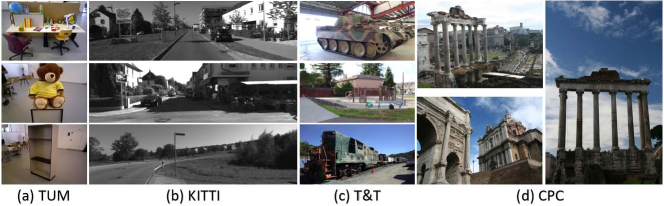
Figure 2: Sample images from the benchmark datasets.

Table 1: Details of the benchmark datasets.

Datasets	#Seq	#Image	Resolution	Baseline	Property
TUM	3	5994	$480\times 640$	short	indoor scenes
KITTI	5	9065	$370\times 1226$	short	street views
T&T	3	922	$1080\times 2048$	wide	outdoor scenes
			$1080\times 1920$
CPC	1	1615	varying	wide	internet photos

5 Experiments

Related research is quite rich, so we mainly focus on evaluating recently proposed algorithms and the widely used methods in this paper. In the following, we introduce the experimental configuration, discuss results, and propose our methods.

5.1 Experimental Setup

Baseline and Comparability.

We set a classic pipeline as the baseline. Specifically, we use DoG [Lowe(2004)] detector and SIFT [Lowe(2004)] descriptor to generate initial correspondences across images by the plain nearest-neighbor search, then prune bad correspondences using Lowe’s ratio test [Lowe(2004)], and finally compute FM estimates and remove outliers using RANSAC [Fischler and Bolles(1981)] with the 8-point algorithm [Hartley(1997)]. For each evaluated algorithm, we incorporate it into the baseline system by replacing its counterpart, and use the overall performance for comparison.

Evaluated Methods.

Firstly, we evaluate four deep learning based local features, including HesAffNet [Mishkin et al.(2018)Mishkin, Radenovic, and Matas] detector and two descriptors (L2Net [Tian et al.(2017)Tian, Fan, Wu, et al.], HardNet++ [Mishchuk et al.(2017)Mishchuk, Mishkin, Radenovic, and Matas]). Besides, two hand-crafted descriptors (DSP-SIFT [Dong and Soatto(2015)] and RootSIFT-PCA [Arandjelovic and Zisserman(2012), Bursuc et al.(2015)Bursuc, Tolias, and Jégou]) are also evaluated, which show high performance in the recent benchmark [Schönberger et al.(2017)Schönberger, Hardmeier, Sattler, and Pollefeys]. Secondly, we evaluate four correspondence pruning algorithms: CODE [Lin et al.(2017)Lin, Wang, Cheng, Yeung, Torr, Do, and Lu], GMS [Bian et al.(2017)Bian, Lin, Matsushita, Yeung, Nguyen, and Cheng], LPM [Ma et al.(2018)Ma, Zhao, Jiang, Zhou, and Guo], and LC [Yi et al.(2018)Yi, Trulls, Ono, Lepetit, Salzmann, and Fua]. Finally, we evaluate two widely used estimators (LMedS [Rousseeuw and Leroy(1987)] and MSAC [Torr and Zisserman(2000)]) and two state-of-the-art alternatives (USAC [Raguram et al.(2013)Raguram, Chum, Pollefeys, Matas, and Frahm] and GC-RANSAC [Barath and Matas(2018)]).

Implementations.

We use VLFeat [Vedaldi and Fulkerson(2010)] library for the implementation of SIFT descriptor and DoG detector, and the threshold is $0.8$ for ratio test [Lowe(2004)]. Matlab functions are used for RANSAC, LMedS, and MSAC implementations, where we limit the maximum iteration as $2000$ for a reasonable speed. Other codes are from authors’ publicly available implementation, where we use the pre-trained models released by authors for deep learning based methods.

Table 2: Experimental results. First, second, third best results are highlighted in color, and the results that are better than the baseline (the first line in each block) performance are highlighted in bold. %Recall represents the overall performance.

Datasets	(a) Local Features					(b) Pruning Methods					(c) Robust Estimators
	Methods	%Recall	%Inlier	%Inlier-m	#Corrs (-m)	Methods	%Recall	%Inlier	%Inlier-m	#Corrs (-m)	Methods	%Recall	%Inlier	%Inlier-m	#Corrs (-m)
TUM	SIFT	57.40	75.33	59.21	65 (316)	RATIO	57.40	75.33	59.21	65 (316)	RANSAC	57.40	75.33	59.21	65 (316)
	DSP-SIFT	53.90	74.89	56.44	66 (380)	GMS	59.20	76.18	69.72	64 (241)	LMedS	69.20	75.24	59.21	158 (316)
	RootSIFT-PCA	58.90	75.65	62.22	67 (306)	LPM	58.90	75.75	64.42	67 (290)	MSAC	52.70	75.12	59.21	63 (316)
	L2Net	58.10	75.49	59.26	66 (319)	LC	54.10	75.96	71.32	57 (203)	USAC	56.50	72.13	59.21	244 (316)
	HardNet++	58.90	75.74	62.07	67 (315)	CODE	62.50	76.95	66.82	3119 (18562)	GC-RSC	30.80	68.13	59.21	272 (316)
	HesAffNet	51.70	75.70	62.06	101 (657)
KITTI	SIFT	91.70	98.20	87.40	154 (525)	RATIO	91.70	98.20	87.40	154 (525)	RANSAC	91.70	98.20	87.40	154 (525)
	DSP-SIFT	92.00	98.22	87.60	153 (572)	GMS	91.70	98.58	95.56	148 (445)	LMedS	91.80	98.25	87.40	263 (525)
	RootSIFT-PCA	92.00	98.23	90.76	156 (514)	LPM	91.50	98.27	92.50	157 (501)	MSAC	91.80	98.12	87.40	153 (525)
	L2Net	91.60	98.21	89.40	156 (520)	LC	89.70	99.44	97.49	96 (267)	USAC	82.70	97.39	87.40	455 (525)
	HardNet++	92.00	98.21	91.25	159 (535)	CODE	92.50	98.32	93.03	4834 (19246)	GC-RSC	56.50	95.00	87.40	487 (525)
	HesAffNet	90.40	98.09	90.64	233 (1182)
T&T	SIFT	70.00	75.20	53.25	85 (795)	RATIO	70.00	75.20	53.25	85 (795)	RANSAC	70.00	75.20	53.25	85 (795)
	DSP-SIFT	75.10	80.20	60.02	90 (845)	GMS	80.90	84.38	77.65	90 (598)	LMedS	83.40	77.26	53.25	398 (795)
	RootSIFT-PCA	77.40	80.55	61.75	89 (738)	LPM	80.70	81.62	66.98	90 (667)	MSAC	64.60	73.27	53.43	84 (799)
	L2Net	70.40	73.76	57.31	93 (799)	LC	76.60	84.01	72.24	77 (512)	USAC	78.80	80.98	53.25	495 (795)
	HardNet++	79.90	81.05	63.61	96 (814)	CODE	89.40	89.14	76.98	782 (9251)	GC-RSC	80.40	78.97	53.25	612 (795)
	HesAffNet	82.50	84.71	70.29	97 (920)
CPC	SIFT	29.20	67.14	48.07	60 (415)	RATIO	29.20	67.14	48.07	60 (415)	RANSAC	29.20	67.14	48.07	60 (415)
	DSP-SIFT	35.20	76.48	56.29	57 (367)	GMS	43.00	85.90	82.37	59 (249)	LMedS	44.00	75.38	48.07	209 (415)
	RootSIFT-PCA	38.20	78.45	59.92	62 (361)	LPM	39.40	78.17	65.98	60 (310)	MSAC	23.00	62.28	48.07	59 (415)
	L2Net	29.60	60.22	50.70	93 (433)	LC	39.40	83.99	72.22	51 (295)	USAC	49.70	80.38	48.07	232 (415)
	HardNet++	40.30	76.73	62.30	69 (400)	CODE	51.00	90.16	78.55	696 (5774)	GC-RSC	53.70	81.15	48.07	269 (415)
	HesAffNet	47.40	84.58	72.22	65 (405)

5.2 Results and Discussion

Tab. 2 reports the experimental results for all methods and datasets. In each block, the first line shows the baseline performance. First, second, third best results are highlighted in color, and the results that are better than the baseline are highlighted in bold. Here, we mainly compare algorithms in terms of %Recall, which reflects the overall performance. In addition, %Inlier shows matching performance, and %Inlier-m shows matching before outlier rejection phase. #Corrs(-m) is used to analyze results instead of performance comparison. The detail about these metrics can be seen in Sec. 3. For performance analyses, we mainly target on concluding the distinctive properties of the best methods instead of a comprehensive comparison of all approaches.

Local Features.

Tab. 2(a) shows the results of local features. The %Recall implies that a) RootSIFT-PCA [Bursuc et al.(2015)Bursuc, Tolias, and Jégou] and HardNet++ [Mishchuk et al.(2017)Mishchuk, Mishkin, Radenovic, and Matas] consistently outperform the baseline, and the latter is better than the former. b) HesAffNet [Mishkin et al.(2018)Mishkin, Radenovic, and Matas] performs best in wide-baseline scenarios (T&T and CPC), although it is degenerate on the TUM dataset. c) DSP-SIFT [Dong and Soatto(2015)] outperforms the baseline on almost all datasets but TUM, and L2Net [Tian et al.(2017)Tian, Fan, Wu, et al.] shows similar performances with the baseline on all datasets.

Correspondence Pruning Methods.

Tab. 2(b) shows the results of pruning methods. It shows that a) CODE [Lin et al.(2017)Lin, Wang, Cheng, Yeung, Torr, Do, and Lu] achieves the state-of-the-art performance on all datasets. b) GMS [Bian et al.(2017)Bian, Lin, Matsushita, Yeung, Nguyen, and Cheng] and LPM [Ma et al.(2018)Ma, Zhao, Jiang, Zhou, and Guo] consistently outperform the baseline methods by pruning bad correspondences effectively, i.e., improving the %Inlier-m and preserving a considerable #Corrs-m in the meanwhile. Here, GMS is better than LPM. c) LC [Yi et al.(2018)Yi, Trulls, Ono, Lepetit, Salzmann, and Fua] can boost the matching accuracy (%Inlier-m) but, for estimation (%Recall), it is degenerate on the short-baseline datasets (TUM and KITTI). Perhaps this is because the provided model is trained on wide-baseline datasets. Also, note that it requires camera intrinsics, which are normally assumed to be unknown for the FM estimation problem.

Robust Estimators.

Tab. 2(c) shows the results of robust estimators. They show: a) LMedS [Rousseeuw and Leroy(1987)] performs best on the first three datasets where images are not as difficult as CPC dataset. This confirms the suggestion by Matlab documentation that LMedS works well when the inlier rate is high enough, e.g., above $50\%$. b) GC-RANSAC [Barath and Matas(2018)] and USAC [Raguram et al.(2013)Raguram, Chum, Pollefeys, Matas, and Frahm] show high performances in wide-baseline scenarios, especially on the challenging CPC dataset. However, they are degenerate in short-baseline scenarios (TUM and KITTI). c) Interestingly, we observe that GC-RANSAC (also USAC) can preserve rich correspondences (%Corrs-m) and prune outliers (%Inlier(-m)) effectively.

Runtime.

As algorithms rely on different operating systems, we use two machines for evaluation: a Linux server L (Intel E5-2620 CPU, NVIDIA Titan Xp GPU) and a Windows laptop W ( Intel i7-3630QM CPU, NVIDIA GeForce GT 650M GPU), where $100$ images from the KITTI dataset are used for testing and the averaged results are reported. Tab. 3 reports the time consumption of algorithms. Descriptors rely on DoG [Lowe(2004)] detector, which (L) takes $238ms$ to extract $1760$ keypoints, and HesAffNet [Mishkin et al.(2018)Mishkin, Radenovic, and Matas] detector extracts $4860$ keypoints. CODE [Lin et al.(2017)Lin, Wang, Cheng, Yeung, Torr, Do, and Lu] (W) takes $2.953s$ to extract $58,675$ keypoints using GPU, and takes $4.068s$ to prune bad correspondences using CPU.

Table 3: Time consumption of evaluated algorithms.

Device	Runtime (seconds)
L	SIFT	DSP-SIFT	RootSIFT-PCA	L2Net	HardNet++	HesAffNet
	0.702	1.762	0.705	2.260	0.002	0.367
W	LPM	GMS	LC	CODE
	0.003	0.001	0.021	4.068
	RANSAC	LMedS	MSAC	USAC	GC-RSC
	0.521	0.528	0.537	0.565	0.788

5.3 Proposed Methods

Drawing inspiration from the results, we propose three practical matching systems and a robust estimator as follows.

Matching Systems.

We first adopt one of the following three pairs of detectors and descriptors for generating putative correspondences:

1. DoG [Lowe(2004)] + RootSIFT-PCA [Bursuc et al.(2015)Bursuc, Tolias, and Jégou]

2. DoG + (HardNet++) [Mishchuk et al.(2017)Mishchuk, Mishkin, Radenovic, and Matas]

3. HesAffNet [Mishkin et al.(2018)Mishkin, Radenovic, and Matas] + (HardNet++)

where we recommend 1, 2 for general scenes and 3 for wide-baseline scenarios. Then, we apply ratio test (the threshold is $0.8$) and GMS [Bian et al.(2017)Bian, Lin, Matsushita, Yeung, Nguyen, and Cheng] to prune bad correspondences. Finally, we use LMedS [Rousseeuw and Leroy(1987)] based estimator for model fitting. Tab. 4 shows the evaluation results, which clearly demonstrate that the recommended systems outperform the baseline, and achieve competitive performances with the state-of-the-art system (CODE [Lin et al.(2017)Lin, Wang, Cheng, Yeung, Torr, Do, and Lu] + LMedS [Rousseeuw and Leroy(1987)]). Note that CODE is several orders of magnitude slower, even GPU is adopted.

Coarse-to-Fine RANSAC.

Tab. 2 shows that GC-RANSAC [Barath and Matas(2018)] and USAC [Raguram et al.(2013)Raguram, Chum, Pollefeys, Matas, and Frahm] prune outliers effectively, although they fail to show consistently high performance on model fitting. To this end, we propose to use GC-RANSAC [Barath and Matas(2018)] for pruning bad matches, and then apply LMedS [Rousseeuw and Leroy(1987)] based estimator for model fitting. Note that USAC is also applicable. In this two-stage framework, the former is used to roughly find the inlier set and the latter to fit the model accurately, so we term the resultant approach Coarse-to-Fine RANSAC (CF-RSC in short). Tab. 5 shows the results of the proposed method in terms of %Recall, where all estimators use the same input, i.e., SIFT [Lowe(2004)] matches with ratio test pruning. It shows that the proposed CF-RSC significantly outperforms other alternatives.

Table 4: Evaluation results of the proposed matching systems.

Datasets	Methods	%Recall	%Inlier	%Inlier-m	#Corrs(-m)
TUM	Baseline	57.40	75.33	59.21	65 (316)
	CODE	67.50	76.04	66.82	9281 (18562)
	RootSIFT-PCA + GMS	67.50	76.13	69.62	124 (248)
	HardNet + GMS	68.60	75.85	69.39	128 (256)
	HesAffNet + GMS	66.40	75.92	67.04	288 (577)
KITTI	Baseline	91.70	98.20	87.40	154 (525)
	CODE	91.90	98.22	93.03	9623 (19246)
	RootSIFT-PCA + GMS	92.50	98.54	95.73	225 (450)
	HardNet + GMS	92.10	98.49	95.43	236 (472)
	HesAffNet + GMS	91.80	98.48	94.18	540 (1079)
T&T	Baseline	70.00	75.20	53.25	85 (795)
	CODE	92.70	87.81	76.98	4626 (9251)
	RootSIFT-PCA + GMS	89.30	85.29	78.69	307 (614)
	HardNet + GMS	92.20	85.52	78.86	343 (686)
	HesAffNet + GMS	90.90	86.16	79.25	412 (824)
CPC	Baseline	29.20	67.14	48.07	60 (415)
	CODE	61.80	89.45	78.55	2890 (5774)
	RootSIFT-PCA + GMS	57.30	88.94	83.70	133 (263)
	HardNet + GMS	60.10	88.34	83.12	149 (298)
	HesAffNet + GMS	60.80	88.72	83.16	182 (362)

Table 5: %Recall of the proposed CF-RSC.

Datasets	RANSAC	LMedS	MSAC	USAC	GC-RSC	CF-RSC
TUM	57.40	69.20	52.70	56.50	30.80	69.30
KITTI	91.70	91.80	91.80	82.70	56.50	92.30
T&T	70.00	83.40	64.60	78.80	80.40	90.70
CPC	29.20	44.00	23.00	49.70	53.70	60.90

6 Conclusions

This paper evaluates the recently proposed local features, correspondence pruning algorithms, and robust estimators using strictly defined metrics in the context of image matching and fundamental matrix estimation. Comprehensive evaluation results on four large-scale datasets provide insights into which datasets are particularly challenging and which algorithms perform well in which scenarios. This can advance the development of related research fields, and it can also help researchers design practical matching systems in different applications. Finally, drawing inspiration from the results, we propose three high-quality image matching systems and a robust estimator, Coarse-to-Fine RANSAC. They achieve remarkable performances and have potentials in a wide range of computer vision tasks.

7 Acknowledgement

The authors would like to thank TuSimple and Huawei Technologies Co. Ltd.

References

- [Agarwal et al.(2011)Agarwal, Furukawa, Snavely, Simon, Curless, Seitz, and Szeliski] Sameer Agarwal, Yasutaka Furukawa, Noah Snavely, Ian Simon, Brian Curless, Steven M Seitz, and Richard Szeliski. Building Rome in a day. Communications of the ACM, 54(10):105–112, 2011.
- [Arandjelovic and Zisserman(2012)] Relja Arandjelovic and Andrew Zisserman. Three things everyone should know to improve object retrieval. In IEEE Conference on Computer Vision and Pattern Recognition (CVPR), pages 2911–2918. IEEE, 2012.
- [Armangué and Salvi(2003)] Xavier Armangué and Joaquim Salvi. Overall view regarding fundamental matrix estimation. Image and Vision Computing, 21(2):205–220, 2003.
- [Balntas et al.(2016)Balntas, Riba, Ponsa, and Mikolajczyk] Vassileios Balntas, Edgar Riba, Daniel Ponsa, and Krystian Mikolajczyk. Learning local feature descriptors with triplets and shallow convolutional neural networks. In British Machine Vision Conference (BMVC), page 3, 2016.
- [Balntas et al.(2017)Balntas, Lenc, Vedaldi, and Mikolajczyk] Vassileios Balntas, Karel Lenc, Andrea Vedaldi, and Krystian Mikolajczyk. HPatches: A benchmark and evaluation of handcrafted and learned local descriptors. In IEEE Conference on Computer Vision and Pattern Recognition (CVPR), pages 5173–5182. IEEE, 2017.
- [Barath and Matas(2018)] Daniel Barath and Jiri Matas. Graph-Cut RANSAC. In IEEE Conference on Computer Vision and Pattern Recognition (CVPR), 2018.
- [Bian et al.(2017)Bian, Lin, Matsushita, Yeung, Nguyen, and Cheng] JiaWang Bian, Wen-Yan Lin, Yasuyuki Matsushita, Sai-Kit Yeung, Tan Dat Nguyen, and Ming-Ming Cheng. GMS: Grid-based motion statistics for fast, ultra-robust feature correspondence. In IEEE Conference on Computer Vision and Pattern Recognition (CVPR), pages 4181–4190. IEEE, 2017.
- [Brown et al.(2011)Brown, Hua, and Winder] Matthew Brown, Gang Hua, and Simon Winder. Discriminative learning of local image descriptors. IEEE Transactions on Pattern Recognition and Machine Intelligence (PAMI), pages 43–57, 2011.
- [Bursuc et al.(2015)Bursuc, Tolias, and Jégou] Andrei Bursuc, Giorgos Tolias, and Hervé Jégou. Kernel local descriptors with implicit rotation matching. In International Conference on Multimedia Retrieval, pages 595–598. ACM, 2015.
- [Choi et al.(1997)Choi, Kim, and Yu] Sunglok Choi, Taemin Kim, and Wonpil Yu. Performance evaluation of RANSAC family. International Journal on Computer Vision (IJCV), 24(3):271–300, 1997.
- [Davison et al.(2007)Davison, Reid, Molton, and Stasse] Andrew J Davison, Ian D Reid, Nicholas D Molton, and Olivier Stasse. MonoSLAM: Real-time single camera slam. IEEE Transactions on Pattern Recognition and Machine Intelligence (PAMI), 29(6):1052–1067, 2007.
- [Dong and Soatto(2015)] Jingming Dong and Stefano Soatto. Domain-size pooling in local descriptors: DSP-SIFT. In IEEE Conference on Computer Vision and Pattern Recognition (CVPR), pages 5097–5106, 2015.
- [Fathy et al.(2011)Fathy, Hussein, and Tolba] Mohammed E Fathy, Ashraf S Hussein, and Mohammed F Tolba. Fundamental matrix estimation: A study of error criteria. Pattern Recognition Letters, 32(2):383–391, 2011.
- [Fischler and Bolles(1981)] Martin A Fischler and Robert C Bolles. Random sample consensus: a paradigm for model fitting with applications to image analysis and automated cartography. Communications of the ACM, 24(6):381–395, 1981.
- [Forster et al.(2014)Forster, Pizzoli, and Scaramuzza] Christian Forster, Matia Pizzoli, and Davide Scaramuzza. SVO: Fast semi-direct monocular visual odometry. In International Conference on Robotics and Automation (ICRA), pages 15–22. IEEE, 2014.
- [Geiger et al.(2012)Geiger, Lenz, and Urtasun] Andreas Geiger, Philip Lenz, and Raquel Urtasun. Are we ready for autonomous driving? the KITTI vision benchmark suite. In IEEE Conference on Computer Vision and Pattern Recognition (CVPR), pages 3354–3361. IEEE, 2012.
- [Hartley and Zisserman(2003)] Richard Hartley and Andrew Zisserman. Multiple view geometry in computer vision. Cambridge university press, 2003.
- [Hartley(1997)] Richard I Hartley. In defense of the eight-point algorithm. IEEE Transactions on Pattern Recognition and Machine Intelligence (PAMI), 19(6):580–593, 1997.
- [Heinly et al.(2012)Heinly, Dunn, and Frahm] Jared Heinly, Enrique Dunn, and Jan-Michael Frahm. Comparative evaluation of binary features. In European Conference on Computer Vision (ECCV), pages 759–773. Springer, 2012.
- [Heinly et al.(2015)Heinly, Schonberger, Dunn, and Frahm] Jared Heinly, Johannes L Schonberger, Enrique Dunn, and Jan-Michael Frahm. Reconstructing the world* in six days*(as captured by the yahoo 100 million image dataset). In IEEE Conference on Computer Vision and Pattern Recognition (CVPR), pages 3287–3295, 2015.
- [Knapitsch et al.(2017)Knapitsch, Park, Zhou, and Koltun] Arno Knapitsch, Jaesik Park, Qian-Yi Zhou, and Vladlen Koltun. Tanks and Temples: Benchmarking large-scale scene reconstruction. ACM Transactions on Graphics (TOG), 36(4):78, 2017.
- [Lacey et al.(2000)Lacey, Pinitkarn, and Thacker] AJ Lacey, N Pinitkarn, and Neil A Thacker. An evaluation of the performance of RANSAC algorithms for stereo camera calibrarion. In British Machine Vision Conference (BMVC), pages 1–10, 2000.
- [Lin et al.(2017)Lin, Wang, Cheng, Yeung, Torr, Do, and Lu] Wen-Yan Lin, Fan Wang, Ming-Ming Cheng, Sai-Kit Yeung, Philip HS Torr, Minh N Do, and Jiangbo Lu. CODE: Coherence based decision boundaries for feature correspondence. IEEE Transactions on Pattern Recognition and Machine Intelligence (PAMI), 2017.
- [Lowe(2004)] David G Lowe. Distinctive image features from scale-invariant keypoints. International Journal on Computer Vision (IJCV), 60(2):91–110, 2004.
- [Luo et al.(2018)Luo, Shen, Zhou, Zhu, Zhang, Yao, Fang, and Quan] Zixin Luo, Tianwei Shen, Lei Zhou, Siyu Zhu, Runze Zhang, Yao Yao, Tian Fang, and Long Quan. GeoDesc: Learning local descriptors by integrating geometry constraints. In European Conference on Computer Vision (ECCV), 2018.
- [Ma et al.(2018)Ma, Zhao, Jiang, Zhou, and Guo] Jiayi Ma, Ji Zhao, Junjun Jiang, Huabing Zhou, and Xiaojie Guo. Locality preserving matching. International Journal on Computer Vision (IJCV), 2018.
- [Mikolajczyk and Schmid(2005)] Krystian Mikolajczyk and Cordelia Schmid. A performance evaluation of local descriptors. IEEE Transactions on Pattern Recognition and Machine Intelligence (PAMI), 27(10):1615–1630, 2005.
- [Mikolajczyk et al.(2005)Mikolajczyk, Tuytelaars, Schmid, Zisserman, Matas, Schaffalitzky, Kadir, and Van Gool] Krystian Mikolajczyk, Tinne Tuytelaars, Cordelia Schmid, Andrew Zisserman, Jiri Matas, Frederik Schaffalitzky, Timor Kadir, and Luc Van Gool. A comparison of affine region detectors. International Journal on Computer Vision (IJCV), 65(1-2):43–72, 2005.
- [Mishchuk et al.(2017)Mishchuk, Mishkin, Radenovic, and Matas] Anastasiia Mishchuk, Dmytro Mishkin, Filip Radenovic, and Jiri Matas. Working hard to know your neighbor’s margins: Local descriptor learning loss. In Neural Information Processing Systems (NIPS), pages 4826–4837, 2017.
- [Mishkin et al.(2018)Mishkin, Radenovic, and Matas] Dmytro Mishkin, Filip Radenovic, and Jiri Matas. Repeatability is not enough: Learning affine regions via discriminability. In European Conference on Computer Vision (ECCV). Springer, 2018.
- [Mur-Artal et al.(2015)Mur-Artal, Montiel, and Tardos] Raul Mur-Artal, Jose Maria Martinez Montiel, and Juan D Tardos. ORB-SLAM: a versatile and accurate monocular slam system. IEEE Transactions on Robotics (TRO), 31(5):1147–1163, 2015.
- [Radenovic et al.(2016)Radenovic, Schönberger, Ji, Frahm, Chum, and Matas] Filip Radenovic, Johannes L Schönberger, Dinghuang Ji, Jan-Michael Frahm, Ondrej Chum, and Jiri Matas. From dusk till dawn: Modeling in the dark. In IEEE Conference on Computer Vision and Pattern Recognition (CVPR), pages 5488–5496, 2016.
- [Raguram et al.(2008)Raguram, Frahm, and Pollefeys] Rahul Raguram, Jan-Michael Frahm, and Marc Pollefeys. A comparative analysis of RANSAC techniques leading to adaptive real-time random sample consensus. In European Conference on Computer Vision (ECCV), pages 500–513. Springer, 2008.
- [Raguram et al.(2013)Raguram, Chum, Pollefeys, Matas, and Frahm] Rahul Raguram, Ondrej Chum, Marc Pollefeys, Jiri Matas, and Jan-Michael Frahm. USAC: a universal framework for random sample consensus. IEEE Transactions on Pattern Recognition and Machine Intelligence (PAMI), 35(8):2022–2038, 2013.
- [Ranftl and Koltun(2018)] René Ranftl and Vladlen Koltun. Deep fundamental matrix estimation. In European Conference on Computer Vision (ECCV), pages 284–299, 2018.
- [Rousseeuw and Leroy(1987)] Peter J Rousseeuw and Annick M Leroy. Robust regression and outlier detection, volume 589. John wiley & sons, 1987.
- [Schönberger and Frahm(2016)] Johannes L Schönberger and Jan-Michael Frahm. Structure-from-motion revisited. In IEEE Conference on Computer Vision and Pattern Recognition (CVPR), pages 4104–4113, 2016.
- [Schönberger et al.(2015)Schönberger, Radenovic, Chum, and Frahm] Johannes L Schönberger, Filip Radenovic, Ondrej Chum, and Jan-Michael Frahm. From single image query to detailed 3d reconstruction. In IEEE Conference on Computer Vision and Pattern Recognition (CVPR), pages 5126–5134, 2015.
- [Schönberger et al.(2017)Schönberger, Hardmeier, Sattler, and Pollefeys] Johannes L Schönberger, Hans Hardmeier, Torsten Sattler, and Marc Pollefeys. Comparative evaluation of hand-crafted and learned local features. In IEEE Conference on Computer Vision and Pattern Recognition (CVPR), pages 6959–6968. IEEE, 2017.
- [Sturm et al.(2012)Sturm, Engelhard, Endres, Burgard, and Cremers] J. Sturm, N. Engelhard, F. Endres, W. Burgard, and D. Cremers. A benchmark for the evaluation of RGB-D SLAM systems. In IEEE International Conference on Intelligent Robots and Systems (IROS), Oct. 2012.
- [Tian et al.(2017)Tian, Fan, Wu, et al.] Yurun Tian, Bin Fan, Fuchao Wu, et al. L2-Net: Deep learning of discriminative patch descriptor in euclidean space. In IEEE Conference on Computer Vision and Pattern Recognition (CVPR), volume 1, page 6, 2017.
- [Torr and Murray(1997)] Philip HS Torr and David W Murray. The development and comparison of robust methods for estimating the fundamental matrix. International Journal on Computer Vision (IJCV), 24(3):271–300, 1997.
- [Torr and Zisserman(2000)] Philip HS Torr and Andrew Zisserman. MLESAC: A new robust estimator with application to estimating image geometry. Computer Vision and Image Understanding (CVIU), 78(1):138–156, 2000.
- [Torr and Zissermann(1997)] Philip HS Torr and A Zissermann. Performance characterization of fundamental matrix estimation under image degradation. Machine Vision and Applications, 9(5-6):321–333, 1997.
- [Vedaldi and Fulkerson(2010)] Andrea Vedaldi and Brian Fulkerson. VLFeat: An open and portable library of computer vision algorithms. In ACM International Conference on Multimedia (ACM MM), pages 1469–1472. ACM, 2010.
- [Wilson and Snavely(2014)] Kyle Wilson and Noah Snavely. Robust global translations with 1DSFM. In European Conference on Computer Vision (ECCV), pages 61–75. Springer, 2014.
- [Yi et al.(2018)Yi, Trulls, Ono, Lepetit, Salzmann, and Fua] Kwang Moo Yi, Eduard Trulls, Yuki Ono, Vincent Lepetit, Mathieu Salzmann, and Pascal Fua. Learning to find good correspondences. In IEEE Conference on Computer Vision and Pattern Recognition (CVPR), 2018.
- [Zhang(1998)] Zhengyou Zhang. Determining the epipolar geometry and its uncertainty: A review. International Journal on Computer Vision (IJCV), 27(2):161–195, Mar 1998. ISSN 1573-1405. 10.1023/A:1007941100561.