Invariants of rational links represented by reduced alternating diagrams

Abstract.

A rational link may be represented by any of the (infinitely) many link diagrams corresponding to various continued fraction expansions of the same rational number. The continued fraction expansion of the rational number in which all signs are the same is called a nonalternating form and the diagram corresponding to it is a reduced alternating link diagram, which is minimum in terms of the number of crossings in the diagram. Famous formulas exist in the literature for the braid index of a rational link by Murasugi and for its HOMFLY polynomial by Lickorish and Millet, but these rely on a special continued fraction expansion of the rational number in which all partial denominators are even (called all-even form). In this paper we present an algorithmic way to transform a continued fraction given in nonalternating form into the all-even form. Using this method we derive formulas for the braid index and the HOMFLY polynomial of a rational link in terms of its reduced alternating form, or equivalently the nonalternating form of the corresponding rational number.

1. Introduction

How to compute the braid index of rational links was first shown by Murasugi [13] more than 25 years ago. This computation became possible because of the discovery of the HOMFLY polynomial $H(a,z)$ [8, 14]. Using this polynomial one could derive the Morton-William-Frank inequality [7, 12]:

$$\textbf{b}(K)\geq(E(K)-e(K))/2+1,$$

where $K$ is a knot or link, $\textbf{b}(K)$ is the braid index of $K$, $E(K)$ is the maximal $a$-power of $H_{K}(a,z)$, $e(K)$ is the minimal $a$-power of $H_{K}(a,z)$, and $H_{K}(a,z)$ is the HOMFLY polynomial of the knot or link $K$. In addition, we have an inequality given by Yamada [16]

$$\textbf{b}(K)\leq s(D_{K}),$$

where $D_{K}$ is any regular diagram of $K$ and $s(D_{K})$ is the number of Seifert circles in $D_{K}$. In the case that one can find a diagram $D$ of a knot or link $K$ such that $s(D)=(E(D)-e(D))/2+1$ holds, it then follows that we must have $s(D)=\textbf{b}(D)$.

When Murasugi [13] first established the braid index of rational links, he did so by using a special diagram $D_{K}$ of the link $K$ that relies on a particular continued fraction expansion using only even integers which is usually highly non minimal. The same special expansion was used by Lickorish and Millet [11, Proposition 14] to present a formula for the HOMFLY polynomial of a rational link. A possible reason for representing rational links with such a special diagram is noted by Duzhin and Shkolnikov [5] who observed that “due to the fact that all blocks are of even length, strands are everywhere counter-directed.”

Unfortunately, this special all-even expansion is not only highly non-minimal, but it also does not exist if both integers in the fraction defining the rational link are odd, in which case one could not apply this method directly and needs to use a diagram of the mirror image of $K$ (which corresponds to a different fraction in which one of the integers is even). Missing are formulas that are stated in terms of minimal (alternating) diagrams or equivalently that can use any fraction of a rational link (even those where both integers are odd).

A first effort in this direction was made by the authors in [4], which contains a formula for the braid index of a rational link $K$, represented by a canonical minimal diagram $D$ of $K$. The proof of the formula is quite different from Murasugi’s approach, the formula itself is in fact just one of the applications of a more general result in [4], which can be applied to compute the braid index of many other knot and link families, including all alternating Montesinos links [4]. The more general validity of the formula also makes it directly applicable to a rational link $K$ (without using its mirror image) even if the numerator and denominator of the corresponding rational number are both odd.

In this paper we take a completely different approach. We develop a general procedure which transforms (when this is possible) a continued fraction representing an alternating link diagram into a continued fraction whose partial denominators are all even. A continued fraction representing an alternating link diagram is a continued fraction in which the signs of the partial denominators do not alternate. We call these nonalternating continued fractions and we partition their partial denominators into primitive blocks. The conversion into all-even form may be performed on these primitive blocks essentially independently (except for some easily predictable propagation of signs). The details of these purely arithmetic manipulations are given in Section 3. With this conversion at hand we have a tool that allows us to transform Murasugi’s formula for the braid index [13] and the Lickorish-Millet formula for the HOMFLY polynomial [11] directly. As explained in Section 4, the primitive blocks also have the property that the crossing sings in an alternating rational link are constant within a block and opposite in adjacent blocks. This observation allows us to phrase our formulas in terms of the crossing signs in a manner that is similar to the main result in [4]. Our new braid index formula is presented in Section 5 and a new HOMFLY polynomial formula is presented in Section 7. The connection between our present braid index formula and the one derived in [4] is explained in Section 6.

The proofs of the results presented in this paper rely on representing the link diagram in all-even form even if they are stated in terms of a minimal representation. Since taking the mirror image does not change the braid index and changes the HOMFLY polynomial only to the extent of a simple substitution $a\mapsto a^{-1}$, the formulas we find remain useful even in the case when the rational link diagram has no all-even representation. It is an interesting question of future research to develop a HOMFLY formula that is independent of the existence of the all-even representation and is comparable in this sense to the braid index formula presented in [4].

2. Finite simple continued fractions

We define a finite simple continued fraction as an expression of the form

(2.1) $$[c_{0},\ldots,c_{n}]=c_{0}+\cfrac{1}{c_{1}+\cfrac{1}{c_{2}+\ddots\cfrac{1}{c_{n-1}+\cfrac{1}{c_{n}}}}},$$

where the partial denominators $c_{0},\ldots,c_{n}$ are integers and $c_{n}\neq 0$. If $c_{n}\neq 0$, we can evaluate the expression using algebra and we obtain a rational number $p/q$. Conversely, as it is well-known, every rational number $p/q$ may be written as a finite continued fraction in such a way, that only the first partial denominator $c_{0}$ may be zero or negative, all other partial denominators are positive. This representation is unique up to the possibility of replacing $[c_{0},\ldots,c_{n-1},1]$ with $[c_{0},\ldots,c_{n-1}+1]$ or, conversely, replacing $[c_{0},\ldots,c_{n}]$ where $c_{n}>1$ with $[c_{0},\ldots,c_{n}-1,1]$.

Equivalently, we may introduce

$$M(c)=\begin{pmatrix}c&1\\ 1&0\\ \end{pmatrix}$$

for each integer $c$, and then the following statement is easily shown by induction on $n$ (cf. [3, p. 205]).

Proposition 2.1.

If the integers $c_{0},c_{1},\ldots,c_{n}$ satisfy $c_{n}\neq 0$, then the value $p/q$ of $[c_{0},\ldots,c_{n}]$ (for the integers $p$ and $q$) is given by

(2.2) $$\begin{pmatrix}p\\ q\\ \end{pmatrix}=M(c_{0})M(c_{1})\cdots M(c_{n})\begin{pmatrix}1\\ 0\\ \end{pmatrix}.$$

Using Equation (2.2) we may extend the definition of the evaluation $[c_{0},c_{1},\ldots,c_{n}]$ to any finite sequence $c_{0},c_{1},\ldots,c_{n}$ of integers. We will set $p/0=\infty$ when $p\neq 0$ and we will leave $0/0$ undefined. Note that, the determinant of $M(c)$ is $-1$, regardless of the value of $c$, and so the vector given in Equation (2.2) is never the null vector.

It is easy to verify directly that extending the evaluation of Equation (2.2) to all finite sequences of integers amounts to adding the following rules to the evaluation of (2.1). We set

$$\frac{p}{0}=\infty\quad\mbox{for $p\neq 0$ and}\quad\frac{p}{\infty}=0\quad\mbox{all $p$}.$$

A key equality whose variants we will be using is the following formula of Lagrange (see Lagrange’s Appendix to Euler’s Algebra [6] cited in [9]),

(2.3) $$[a,-b]=a-\frac{1}{b}=a-1-\frac{1}{1+\frac{1}{b-1}}=[a-1,1,b-1].$$

A slightly generalized variant of (2.3) is the following.

Proposition 2.2.

For $\delta\in\{-1,1\}$, any generalized finite simple continued fraction $[c_{0},\ldots,c_{n}]$ satisfies

$$[c_{0},\ldots,c_{i},\ldots,c_{j},\ldots,c_{n}]=[c_{0},\ldots,c_{i}+\delta,-\delta,\delta-c_{i+1},-c_{i+2},\ldots,-c_{j},\ldots,-c_{n}].$$

This is a direct consequence of the equation

$$M(c_{i})M(c_{i+1})\begin{pmatrix}p\\ q\\ \end{pmatrix}=M(c_{i}+\delta)M(-\delta)M(\delta-c_{i+1})\begin{pmatrix}\delta p\\ -\delta q\\ \end{pmatrix}$$

that holds for any pair of numbers $(p,q)$. The direct verification is left to the reader.

In our applications most of the time we will be interested in finite simple continued fractions satisfying $c_{1}\cdots c_{n}\neq 0$.

Definition 2.3.

We call a finite simple continued fraction $[c_{0},c_{1},\ldots,c_{n}]$ nonsingular if it satisfies $c_{1}\cdots c_{n}\neq 0$, otherwise we call it singular.

Applying Proposition 2.2 to a nonsingular $[c_{0},c_{1},\ldots,c_{n}]$ results in a singular continued fraction only if $c_{i}=-\delta$ or $c_{i+1}=\delta$. In all of these situations we may return to nonsingular finite continued fractions by using the following rule.

Lemma 2.4.

We have

$$[c_{0},c_{1},\ldots,c_{j-1},0,c_{j+1},\ldots,c_{n}]=[c_{0},c_{1},\ldots,c_{j-1}+c_{j+1},\ldots,c_{n}].$$

This is a direct consequence of $M(c_{i-1})M(0)M(c_{i+1})=M(c_{i-1}+c_{i+1})$. In the case when $c_{i}=-\delta$, Proposition 2.2 yields

$$[c_{0},\ldots,c_{i-1},-\delta,c_{i+1}\ldots,c_{j},\ldots,c_{n}]=[c_{0},\ldots,c_{i-1},0,-\delta,\delta-c_{i+1},\ldots,-c_{j},\ldots,-c_{n}].$$

Combining this equation with Lemma 2.4 we obtain

$$[c_{0},\ldots,c_{i-1},-\delta,c_{i+1}\ldots,c_{j},\ldots,c_{n}]=[c_{0},\ldots,c_{i-1}-\delta,\delta-c_{i+1},\ldots,-c_{j},\ldots,-c_{n}].$$

Using Proposition 2.2 and Lemma 2.4 we may transform any finite simple continued fractions in one of the two standard forms as defined in Definition 2.5 below.

Definition 2.5.

A finite simple continued fraction $[c_{0},\ldots,c_{n}]$ is in nonalternating denominator form if $c_{1}\cdots c_{n}\neq 0$, the integers $c_{1},\ldots,c_{n}$ all have the same sign, and $c_{0}$ is either zero or has the same sign as all the other $c_{i}$-s. On the other hand, a finite continued fraction $[c_{0},\ldots,c_{n}]$ is in even denominator form if $c_{1}\cdots c_{n}\neq 0$ and the integers $c_{0},\ldots,c_{n-1}$ are all even integers.

The following statement is a variant of the well-known uniqueness result on the standard continued fraction expansion of a rational number.

Lemma 2.6.

Every rational number $p/q$ has a representation in the nonalternating denominator form. This form is unique up to the possibility of replacing $[c_{0},\ldots,c_{n}]$ with $[c_{0},\ldots,c_{n}-1,1]$ when $c_{n}>1$ or with $[c_{0},\ldots,c_{n}+1,-1]$ when $c_{n}<-1$.

The nonalternating representations of a positive and a negative rational number of the same absolute value are connected by the obvious equality $[-c_{0},\ldots,-c_{n}]=(-1)\cdot[c_{0},\ldots,c_{n}]$.

The following statement is a generalization of the observation made in [5, Lemma 2]. Its proof is essentially the same as that given in [5, Lemma 2].

Lemma 2.7.

Every rational number $p/q$ has a unique representation $[c_{0},\ldots,c_{n}]$ as a finite continued fraction in an even denominator form. The partial denominator $c_{n}$ is even if and only if the product $pq$ is even.

3. Converting the nonalternating denominator form into the even denominator form

Lemma 3.1.

Assume there is an $i$ such that three consecutive partial denominators $c_{i}$, $c_{i+1}$ and $c_{i+2}$ in the nonsingular simple finite continued fraction $[c_{0},\ldots,c_{n}]$ have the same sign as $\delta\in\{-1,1\}$. Then the continued fraction, obtained from $[c_{0},\ldots,c_{n}]$ by the following procedure, has the same evaluation as $[c_{0},\ldots,c_{n}]$:

1. Replace $c_{i}$ with $c_{i}+\delta$ and $c_{i+2}$ with $c_{i+2}+\delta$.

2. Replace $c_{i+1}$ with $|c_{i+1}|-1$ copies of $2$. (In particular, simply remove $c_{i+1}$ if it is equal to $\delta$).

3. Keep the sign of $c_{i}+\delta$ and replace each subsequent sign in such a way that signs alternate up to and including the changed copy of $c_{i+2}$;

4. Replace $c_{j}$ with $(-1)^{|c_{i+1}|}\cdot c_{j}$ for each $j>i+2$.

Proof.

We proceed by induction on $|c_{i+1}|$. If $c_{i+1}=\delta$ then the statement may be obtained from Proposition 2.2 using $-\delta$ and replacing $[\ldots c_{i},\delta,c_{i+1}\ldots]=[\ldots c_{i},\delta-\delta,\delta,-\delta-c_{i+1},-c_{i+2}\ldots]=[\ldots c_{i}+\delta,-\delta-c_{i+1},-c_{i+2}\ldots].$ Assume the statement is true for $|c_{i+1}|=k$ and assume $|c_{i+1}|=k+1$. Let $\delta=\operatorname{sign}(c_{i+1})$. Applying Proposition 2.2 once yields

$$[\ldots,c_{i},c_{i+1},c_{i+2},\ldots,c_{j},\ldots,c_{n}]=[\ldots,c_{i}+\delta,-\delta,\delta-c_{i+1},-c_{i+2},\ldots,-c_{j},\ldots,-c_{n}].$$

Observe that in the resulting continued fraction, the consecutive partial denominators $-\delta,\delta-c_{i+1},$ $-c_{i+2}$ all have the same sign as $-\delta$ and the absolute value of $\delta-c_{i+1}$ is $k$. Applying the induction hypothesis to these three consecutive partial denominators we obtain that our continued fraction has the same evaluation as

$$[\ldots,c_{i}+\delta,-2\cdot\delta,2\cdot\delta,\ldots,(-1)^{k}\cdot 2\cdot\delta,(-1)^{k+1}(c_{i+2}+\delta),\ldots,(-1)^{k+1}c_{j},\ldots,(-1)^{k+1}c_{n}].$$

∎

Proposition 3.2.

Assume a simple continued fraction $[c_{0},\ldots,c_{n}]$ contains a contiguous subsequence $c_{m},c_{m+1},\ldots,c_{m+2k}$ of partial denominators, satisfying the following conditions:

1. the integers $c_{m},c_{m+1},\ldots,c_{m+2k}$ all have the same sign $\delta$;

2. $c_{m}$ and $c_{m+2k}$ are odd;

3. $c_{m+2i}$ is even for $1\leq i\leq k-1$.

Then the continued fraction, obtained by the following transformation, has the same evaluation:

1. replace $c_{m}$ with $c_{m}+\delta$ and $c_{m+2k}$ with $c_{m+2k}+\delta$;

2. for each $i\in\{1,\ldots,k-1\}$ replace $c_{m+2i}$ with $c_{m+2i}+2\delta$;

3. for each $i\in\{1,\ldots,k\}$ replace $c_{m+2i-1}$ with $|c_{m+2i-1}|-1$ copies of $2$;

4. keep the sign of $c_{m}+\delta$ and replace each subsequent sign in such a way that signs alternate up to and including the changed copy of $c_{m+2k}$;

5. for each $j>m+2k+1$ we replace $c_{j}$ with $(-1)^{|c_{m+1}|+|c_{m+3}|+\cdots+|c_{m+2k-1}|}\cdot c_{j}$.

Proof.

To prove this we repeatedly use Lemma 3.1. We explain the principle using an example given by the equality

$$[1,2,\mathbf{3},4,\mathbf{2},1,\mathbf{6},3,\mathbf{5},3]=[1,2,\mathbf{4},-2,2,-2,\mathbf{4},-\mathbf{8},2,-2,\mathbf{6},3].$$

In this example, $m=2$ and $k=3$. To help keep track of the strings of entries inserted between $c_{2},c_{4},c_{6}$ and $c_{8}$, these are marked in bold. We replace $c_{3},c_{5}$ and $c_{7}$ by alternating strings of 2’s. As a first step we apply Lemma 3.1 to $c_{m},c_{m+1},c_{m+2}$. Thus we obtain that our continued fraction has the same evaluation as

$$[\ldots,c_{m}+\delta,-2\delta,2\delta,\ldots,(-1)^{|c_{m+1}|-1}2\delta,(-1)^{|c_{m+1}|}(c_{m+2}+\delta),\ldots,(-1)^{|c_{m+1}|}c_{j},\ldots,(-1)^{|c_{m+1}|}c_{n}].$$

In our example

$$[1,2,\mathbf{3},4,\mathbf{2},1,\mathbf{6},3,\mathbf{5},3]=[1,2,\mathbf{4},-2,2,-2,\mathbf{3},1,\mathbf{6},3,\mathbf{5},3].$$

Next we apply Lemma 3.1 to $(-1)^{|c_{m+1}|}(c_{m+2}+\delta),(-1)^{|c_{m+1}|}c_{m+3},(-1)^{|c_{m+1}|}c_{m+4}$. This results in replacing $(-1)^{|c_{m+1}|}(c_{m+2}+\delta)$ with $(-1)^{|c_{m+1}|}(c_{m+2}+2\delta)$, $(-1)^{|c_{m+1}|}c_{m+3}$ with a sequence of length $|c_{m+3}|-1$ in which copies of $2$ and $-2$ alternate, and $(-1)^{|c_{m+1}|}c_{m+3}$ with $(-1)^{|c_{m+1}|+|c_{m+3}|}(c_{m+3}+\delta)$. All partial denominators after this one are multiplied by $(-1)^{|c_{m+3}|}$. In our example we obtain

$$[1,2,\mathbf{3},4,\mathbf{2},1,\mathbf{6},3,\mathbf{5},3]=[1,2,\mathbf{3},-2,2,-2,\mathbf{4},\mathbf{-7},-3,\mathbf{-5},-3].$$

Note that $c_{5}=1$ is replaced with an empty sequence. We continue in a similar fashion, applying Lemma 3.1 to the consecutive partial denominators $(-1)^{|c_{m+1}|+|c_{m+3}|+\cdots+|c_{m+2i-1}|}(c_{m+2i}+\delta)$, $(-1)^{|c_{m+1}|+|c_{m+3}|+\cdots+|c_{m+2i-1}|}c_{m+2i+1}$ and $(-1)^{|c_{m+1}|+|c_{m+3}|+\cdots+|c_{m+2i-1}|}c_{m+2i+2}$ for $i=1,2,\ldots,k-1$. ∎

Definition 3.3.

We say that a subsequence of consecutive partial denominators $(c_{m},\ldots,c_{m+2k})$ in a nonsingular finite simple continued fraction $[c_{0},\ldots,c_{n}]$ is a primitive block if it satisfies one of the following criteria:

1. $k=0$ and $c_{m}$ is even;

2. $k\geq 1$ and $(c_{m},\ldots,c_{m+2k})$ satisfies the hypotheses in Proposition 3.2;

3. $k=0$, $m=n$ and $c_{n}$ can be odd or even.

We say that a finite simple continued fraction $[c_{0},c_{1},\ldots,c_{n}]$ has a primitive block decomposition if the sequence of its partial denominators may be written as a concatenation of primitive blocks. We will say a primitive block is trivial if $k=0$, otherwise we say it is nontrivial. We will also call a type (3) trivial primitive block exceptional.

Remark 3.4.

A primitive block decomposition, if it exists, allows us to use Proposition 3.2 to rewrite a continued fraction in even denominator form. Indeed, when we apply Proposition 3.2 to a nontrivial primitive block $(c_{m},\ldots,c_{m+2k})$, the sign of each $c_{i}$ satisfying $i<m$ remains unchanged, and all $c_{i}$ satisfying $i>2m+1$ get multiplied by the same power of $(-1)$. Hence the other primitive blocks of the continued fraction remain primitive blocks, whereas the nontrivial primitive block $(c_{m},\ldots,c_{m+2k})$ is replaced by a concatenation of trivial primitive blocks. Applying Proposition 3.2 repeatedly we may replace all nontrivial primitive blocks by a concatenation of trivial primitive blocks. These contain even integers, except for the last one, if that primitive block is exceptional.

Example 3.5.

The rational number $1402/1813$ has the nonalternating simple continuous fraction expansion $[0,1,3,2,2,3,5,1,3]$. This has the primitive block decomposition $[0,1,3,2,2,3;5,1,3]$ (here primitive blocks are separated by semi-colons). By Proposition 3.2, we have

$$[0,1,3,2,2,3;5,1,3]=[0,2,-2,2,-4,2,-4;-5,-1,-3]=[0,2,-2,2,-4,2,-4;-6,4].$$

Proposition 3.6.

If the primitive block decomposition of a finite simple continued fraction $[c_{0},\ldots,c_{n}]$ exists, then it is unique.

Proof.

Let $[c_{0},\ldots,c_{n}]$ be a finite simple continued fraction with a primitive block decomposition. We show this primitive block decomposition is unique. The statement may be shown by induction on $n$. For $n=0$ the statement is obvious. For $n>0$ the partial denominator $c_{0}$ is in a trivial primitive block by itself if and only if $c_{0}$ is even. In that case we may apply the induction hypothesis to $[c_{1},\ldots,c_{n}]$. If $c_{0}$ is odd then it is contained in a nontrivial primitive block that begins with $c_{0}$. By the definition of a nontrivial primitive block, the right and of this block can be only at $c_{2k}$ where $k$ is the least positive integer $i$ such that $c_{2i}$ is odd and of the same sign as $c_{0}$. We may apply the induction hypothesis to $[c_{2k+1},\ldots,c_{n}]$. ∎

Remark 3.7.

The proof of Proposition 3.6 amounts to providing a recursively defined algorithm that finds the unique primitive block decomposition given that such a decomposition exists. Assume that $[c_{0},\ldots,c_{n}]$ is a nonalternating simple continuous fraction expansion:

1. If $c_{0}$ is even, put it into a trivial primitive block, and proceed recursively on $[c_{1},\ldots,c_{n}]$.

2. If $c_{0}$ is odd and $n=0$ then $c_{0}$ is in an exceptional trivial primitive block.

3. If $c_{0}$ is odd and $n>0$ then the nontrivial primitive block containing $c_{0}$ ends at the first odd $c_{2k}$, and we proceed recursively on $[c_{2k+1},\ldots,c_{n}]$.

Next we need to show that for a rational number $p/q$ we can construct a primitive block decomposition.

Theorem 3.8.

Every nonzero rational number $p/q$ may be written in two ways as a finite simple continued fraction in a nonalternating form. Exactly one of of these nonalternating forms has a primitive block decomposition. This primitive block decomposition contains no exceptional trivial primitive block if and only if $pq$ is even.

Proof.

The first sentence recalls Lemma 2.6. What we need to show is that exactly one of the nonalternating forms has a primitive block decomposition. Note that, for $p/q=0$ the only way to write it in nonalternating form is $p/q=[0]$ where $0$ is a trivial primitive block.

From now on, without loss of generality, we may assume $p/q>0$. Such a continued fraction can be written in a nonalternating form in exactly two ways: as $[c_{0},c_{1},\ldots,c_{n}]$ satisfying $c_{0}\geq 0$, $c_{1}\cdots c_{n}>0$ and $c_{n}>1$, or as $[c_{0},c_{1},\ldots,c_{n-1},c_{n}-1,1]$.

Case 1: $[c_{0},c_{1},\ldots,c_{n}]$ has a primitive block decomposition. By Proposition 3.6 this decomposition is unique. We need to show that $[c_{0},c_{1},\ldots,c_{n-1},c_{n}-1,1]$ cannot have a primitive block decomposition. If $c_{n}$ is even then it is contained in a trivial primitive block by itself and $[c_{0},c_{1},\ldots,c_{n-1}]$ has a primitive block decomposition with no exceptional block at $c_{n-1}$. Then the partial denominator $c_{n}-1$ is an odd number that has to be the left end of a nontrivial primitive block, that has no right end in $[c_{0},c_{1},\ldots,c_{n-1},c_{n}-1,1]$. If $c_{n}$ is odd then there are two choices. Either $c_{n}$ is the right end of a block that is not exceptional or $c_{n}$ is an exceptional block. In either case the last block in $[c_{0},c_{1},\ldots,c_{n-1},c_{n}-1,1]$ does not have the correct format and $[c_{0},c_{1},\ldots,c_{n-1},c_{n}-1,1]$ cannot have a primitive block decomposition.

Case 2: $[c_{0},c_{1},\ldots,c_{n}]$ has no primitive block decomposition. We need to show that $[c_{0},c_{1},\ldots,c_{n-1},$ $c_{n}-1,1]$ has a primitive block decomposition. The algorithm described in Remark 3.7 applied to $[c_{0},c_{1},\ldots,c_{n}]$ finds an $m<n$ such that $[c_{0},\ldots,c_{m-1}]$ has a primitive block decomposition with no exceptional trivial primitive block at the end, $c_{m}$ is odd but $c_{m+2i}$ is even for all $m+2i\leq n$. If $n-m$ is even, say $n=m+2k$ then $c_{m},c_{m+1},\ldots,c_{m+2k}-1$ is a nontrivial primitive block in $[c_{0},\ldots,c_{n-1},c_{n}-1,1]$ and the last partial denominator $1$ belongs to an exceptional trivial primitive block. If $n-m$ is odd, say $n=m+2k+1$ then $c_{m},c_{m+1},\ldots,c_{m+2k+1}-1,1$ is a nontrivial primitive block in $[c_{0},\ldots,c_{n-1},c_{n}-1,1]$.

So far we have shown that every rational number may be uniquely written into a nonalternating form that has a primitive block decomposition. The second half of the statement is a direct consequence of Lemma 2.7 and Remark 3.4. ∎

Example 3.9.

As seen in Example 3.5, the nonalternating simple continuous fraction expansion of $1402/1813$ is $[0,1,3,2,2,3,5,1,3]$, which has the primitive block decomposition $[0,1,3,2,2,3;5,1,3]$. The other nonalternating simple continued fraction decomposition is $[0,1,3,2,2,3,5,1,2,1]$, which has no primitive block decomposition: the algorithm described in Remark 3.7 would yield the blocks $0$ and $1,3,2,2,3,$ and the block starting at $5$ is incomplete.

4. Transforming rational links into all-even form

We encode an unoriented rational link diagram by a continued fraction $p/q=[0,a_{1},a_{2},\ldots,a_{n}]$ whose evaluation has absolute value at most one and satisfies $a_{1}\cdots a_{n}\neq 0$, where the numbers $|a_{1}|,\ldots,|a_{n}|$ are the numbers of consecutive half-turn twists in the twistboxes $B_{1},\ldots,B_{n}$ following the sign convention as shown in Figure 1 (without the orientation of the strands).

Figure 1. Without the orientation: the sign convention used to define the standard form of non-oriented rational links; With orientation: preferred standard form of oriented rational links.

We denote the link presented in this form by the symbol $b(q,p)$ or by the vector $(a_{1},a_{2},\ldots,a_{n})$, and call such a diagram a standard diagram of the unoriented rational link. Notice that the left end of the diagram is fixed, the closing on the right end depends on the parity of $n$. Our choice of twisting signs agrees with [1, 3], but some articles use the mirror image [5]. Since the braid index is an invariant of oriented links, we will need to consider the rational links with orientation. Once a rational link $b(q,p)$ is given an orientation, the crossings in it also have signs known as crossing sign in knot theory given by the convention shown in Figure 2, which is not to be confused with the signs of the half-turn twists in the twistboxes in Figure 1.

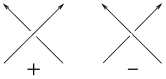
Figure 2. The crossing sign convention at a crossing in an oriented link diagram.

In order to avoid this confusion, in the rest of this paper, we will call the sign given in Figure 1 the twist sign and the sign given by Figure 2 the crossing sign (its usual name in knot theory). We will denote the twist sign of the crossings in twistbox $B_{i}$ (corresponding to $a_{i}$ in $b(q,p)=(a_{0},a_{1},...,a_{n})$) by $\operatorname{sign}_{t}(a_{i})$ and denote the crossing sign of these crossings by $\varepsilon(a_{i})$. Note that the twist sign is given by the formula

(4.1) $$\operatorname{sign}_{t}(a_{i})=(-1)^{i-1}\operatorname{sign}(a_{i}).$$

If there is a need to indicate the crossing sign and the twist sign of the crossings corresponding to an $a_{i}$ entry in a twistbox simultaneously, then we will indicate the twist sign by placing a $+$ or $-$ in front of the number $a_{i}$ and indicate the crossing sign by placing a superscript $+$ or $-$ to $a_{i}$. An example is given in Figure 3. Notice that in general, a rational link diagram in its standard form is not necessarily alternating. In fact, $b(q,p)=(a_{0},a_{1},...,a_{n})$ is an alternating diagram if and only if the continued fraction expansion $[a_{0},a_{1},...,a_{n}]$ is in nonalternating denominator form. From this it follows that every rational link has an alternating link diagram, see [1, 3].

Figure 3. The crossing sign convention for crossings in an oriented link diagram: the signs in front of the $a_{j}$’s indicate which strand is on top as indicated in Figure 1, while the $+$ or $-$ in the superscript indicate the crossing sign given by Figure 2. Shown is the example $[0,2^{-},-3^{+},-1^{-},3^{+},3^{+}]$.

Since we are interested in the braid index and the HOMFLY polynomial of a rational link we need to consider rational links as oriented links. The classification of these links can be found in [1] and is due to Schubert [15].

Theorem 4.1.

$b(q,p)$ and $b(q^{\prime},p^{\prime})$ are equivalent as oriented links if and only if $q=q^{\prime}$ and $p^{\pm 1}\equiv p^{\prime}\mod(2q)$, and are equivalent as unoriented links if and only if $q=q^{\prime}$ and $p^{\pm 1}\equiv p^{\prime}\mod(q)$.

Rational links are invertible and therefore we will orient the lowermost strand from the right to the left (as indicated by solid arrows) without loss of generality. If the orientation of the top strand at left side of the link diagram in its standard form is as shown in Figure 1 (indicated by the hollow arrow), then we say that the link diagram is in a preferred standard form and we will denote by $\tilde{b}(q,p)$ the corresponding link $b(q,p)$ if we want to emphasize that $b(q,p)$ is given by diagram is in preferred standard form. It is important to note that the braid index formula obtained in [13] (Proposition 5.2) is based on preferred standard forms of rational links. As to the HOMFLY polynomial, the result of Lickorish and Millett [11, Proposition 14] we use is stated in terms of the Conway notation [2], but we rephrased it in Proposition 7.1 below as a statement on link diagrams in preferred standard form.

Theorem 4.1 needs some more explanation for oriented links. In the case that $b(q,p)$ has two components, we have two choices for the orientation of the second component (namely the one that does not contain the bottom strand of the diagram), and one and only one such choice would produce a preferred standard diagram $\tilde{b}(q,p)$. By the procedure shown in Figure 4, we can convert any rational link (or knot) that is not in preferred standard form to a preferred standard form representation: first we fold up the part shown with a dashed line in the upper right corner and then we fold down the entire diagram, applying a spatial $180$ degree rotation that changes the twist sign of all crossings. In Figure 4 the continued fraction representing the original link (disregarding the orientation) is $5/18=[0,3,1,1,2]$, after the transformation we obtain the link represented by the continued fraction $-13/18=[0,-1,-2,-1,-1,-2]$. The second continued fraction is obtained from the first by replacing $3$, the first nonzero partial denominator, with the sequence $1,2$ and then taking the negative of all partial denominators. We note that $p=-5$ and $p^{\prime}=-13$ do not satisfy $p^{\pm 1}\equiv p^{\prime}\mod(2q)$. We resolve this problem by assuming that in the case of oriented rational links we are always given the preferred standard form $\tilde{b}(q,p)$ by a vector $(a_{1},a_{2},\ldots,a_{n})$. That is the link $\tilde{b}(18,5)$ given by $5/18=[0,3,1,1,2]$ must have the second component oriented differently than shown in Figure 4. Given $\tilde{b}(q,p)$ the other choice of orientation produces $\tilde{b}(q,-(q-p))$, which is usually a different link type than $\tilde{b}(q,p)$ by Theorem 4.1. In the example of Figure 4 $\tilde{b}(q,-(q-p))=\tilde{b}(18,-13)$ is shown on the bottom right.

This observation may be generalized as follows.

Lemma 4.2.

If $p/q=[0,c_{1},c_{2},\ldots,c_{n}]$ satisfies $|c_{1}|>1$ and $c_{1}\cdots c_{n}\neq 0$ then $1-p/q=(q-p)/q=[0,\operatorname{sign}(c_{1}),c_{1}-\operatorname{sign}(c_{1}),c_{2},\ldots,c_{n}]$. Moreover if $\tilde{b}(q,p)$ is given by the vector $(c_{1},c_{2},\ldots,c_{n})$ then the vector $(\operatorname{sign}(c_{1}),c_{1}-\operatorname{sign}(c_{1}),c_{2},\ldots,c_{n})$ gives the mirror image of $\tilde{b}(q,-(q-p))$.

Note that the operation $p/q\mapsto 1-p/q$ is an involution and that the involution described in Lemma 4.2 above is somewhat similar to the involution described in Lemma 2.6.

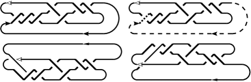
Figure 4. The procedure of changing a two component rational link in a non-preferred standard form to a preferred standard form.

Define the sign of a twistbox $B_{i}$ as the crossing sign of all crossings in it and denote it (by abuse of notation) by $\varepsilon(B_{i})$. Under the assumption that $b(q,p)$ is in a preferred standard form and that $a_{i}>0$ for all $i$ (hence $\varepsilon(B_{1})=+1$), we note that the signs of adjacent twistboxes are related by the automaton shown in Figure 5. (If $a_{i}>0$ but $\varepsilon(B_{1})=-1$ then the diagram is not in a preferred standard form and we would need to change to $\tilde{b}(q,q-p)$.) Inspecting the signs of the crossings in the states of the automaton, we obtain the following result.

\begin{picture}(3924.0,3987.0)(4339.0,-4573.0)\end{picture}

Figure 5. Automaton, parsing the signs of crossings in an alternating link. $o$ and $e$ stand for an odd or even number of crossings in a twistbox respectively.

Theorem 4.3.

Suppose $\tilde{b}(q,p)$ is represented by a nonalternating continued fraction $p/q=[0,a_{1},$ $\ldots,a_{n}]$ that has a primitive block decomposition with no exceptional primitive block. Then twistboxes associated with the same primitive block have the same sign, while the twistboxes associated with adjacent primitive blocks have opposite signs.

Proof.

Let the diagram $D$ be given by the vector $(a_{1},\ldots,a_{n})$. (i) Let $(a_{1},\ldots,a_{1+2k})$ be the first primitive block. Without loss of generality we may assume $a_{i}>0$ for all $i$, the case $a_{i}<0$ for all $i$ is completely analogous. This means that $B_{1}$ is involving the middle two strings of the preferred standard diagram as shown in top middle of Figure 5. If $a_{1}$ is even then it is the only element of its primitive block ($k=0$) and $\varepsilon(B_{2})=-1$. The partial denominator $a_{2}$ corresponds to the bottom center state of Figure 5 and therefore $\varepsilon(a_{2})=-1$. If $a_{1}$ is odd, then it is the first element of a nonsingleton primitive block. We have $\varepsilon(B_{2})=1$, $a_{2}$ corresponds to the top right state in the automaton and $\varepsilon(a_{2})=1$. The subsequent partial denominators correspond to twistboxes filled with positive crossings, as long as we oscillate between the top right and the bottom right states of Figure 5, and we reach the first negative state exactly when we leave the bottom right state moving left. This corresponds exactly to finishing the primitive block containing $a_{1+2k}$ with $a_{1+2k})$ odd and $\varepsilon(B_{2+2k})=-1$ corresponds to the bottom center state of Figure 5.

(ii) Let $(a_{m},\ldots,a_{m+2k})$ be the second primitive block starting at the bottom center state of Figure 5. If $a_{m}$ is even then it is the only element of its primitive block ($k=0$) and $\varepsilon(B_{m+1})=1$. The partial denominator $a_{m+1}$ corresponds to the top center state of Figure 5. If $a_{m}$ is odd, then it is the first element of a nonsingleton primitive block, we have $\varepsilon(B_{m+1})=-1$ and $a_{m+1}$ corresponds to the bottom left state in the automaton. The subsequent partial denominators will all label twistboxes filled with negative crossings, as long as we oscillate between the bottom left and the top left states of Figure 5, and we reach the first positive state exactly when we leave the top left state moving right. This corresponds exactly to finishing the primitive block containing $a_{m+2k}$ with $a_{m+2k})$ odd and $\varepsilon(B_{m+2k+1})=1$ corresponds to the top center state of Figure 5.

The theorem follows by induction on the number of blocks. ∎

Theorem 4.4.

Suppose $\tilde{b}(q,p)$ is represented by a nonalternating continued fraction $p/q=[0,a_{1},\ldots,$ $a_{n}]$ that has a primitive block decomposition with no exceptional primitive block. For each $i\in\{1,\ldots,n\}$ define $\tau_{(}i)$ by

$$\tau(i)=i-1-\mid\{j\leq i\>:\>\varepsilon(a_{j})\neq\varepsilon(a_{j-1})\mbox{ or $j=1$ and $a_{1}$ is even}\}\mid+\sum_{{j<i\atop\varepsilon(a_{j})=\varepsilon(a_{j-1})=(-1)^{j}}}(a_{j}-2).$$

Then the all-even continued fraction representation of $p/q$ may be obtained by replacing each $a_{i}$ as follows.

1. If $a_{1}$ is even, keep it, if it is odd, replace it with $a_{1}+\operatorname{sign}(a_{1})$.

2. If $\varepsilon(a_{i})\neq\varepsilon(a_{i-1})$ then replace $a_{i}$ with $(-1)^{\tau(i)}\cdot a_{i}$ if $a_{i}$ is even and with $(-1)^{\tau(i)}\cdot(a_{i}+\operatorname{sign}(a_{1}))$ if $a_{i}$ is odd.

3. If $\varepsilon(a_{i})=\varepsilon(a_{i-1})=(-1)^{i-1}\cdot\operatorname{sign}(a_{1})$ then replace $a_{i}$ with $(-1)^{\tau(i)}\cdot(a_{i}+\operatorname{sign}(a_{1}))$ if $a_{i}$ is odd and with $(-1)^{\tau(i)}\cdot(a_{i}+2\cdot\operatorname{sign}(a_{1}))$ if $a_{i}$ is even.

4. If $\varepsilon(a_{i})=\varepsilon(a_{i-1})=(-1)^{i}\cdot\operatorname{sign}(a_{1})$ then replace $a_{i}$ with the sequence

   $$(-1)^{\tau(i)}\cdot\operatorname{sign}(a_{1})\cdot 2,(-1)^{\tau(i)}\cdot\operatorname{sign}(a_{1})\cdot(-2),\ldots(-1)^{\tau(i)}\cdot\operatorname{sign}(a_{1})\cdot(-1)^{|a_{i}|-2}\cdot 2$$

   of length $|a_{i}|-1$.

Example 4.5.

Using the example of Proposition 3.2 we have the link $\tilde{b}(49654,34651)$ given by $[0,+1^{+},+2^{+},+3^{+},+4^{-},+2^{+},+1^{-},+6^{-},+3^{-},+5^{+},+3^{+}]$. Applying the procedure given by Theorem 4.4 we have $\operatorname{sign}(a_{1})=+1$, $\tau(2)=1,\tau(3)=\tau(4)=\tau(5)=\tau(6)=2,\tau(7)=3,\tau(8)=8,\tau(9)=9,\tau(10)=9$. This will result in the even denominator form $[0,2,-2,4,4,2,2,-2,2,-2,2,-2,4,6,-2,$ $2]$.

Proof.

The states of the automaton shown in Figure 5 indicate the position of each $a_{i}$ in its primitive block: the two middle states correspond to a last element of a primitive block, the upper right and lower left states correspond to $a_{i}$ being in an odd (but not last) position of a block of odd length, the lower right and upper left states correspond to $a_{i}$ being in an even position in a block of odd length. (We associate to each $a_{i}$ the state reached after reading $a_{i}$.) These states are also identifiable if we know the crossing signs in the twistboxes associated to $a_{i-1}$ and $a_{i}$ and we also know the parity of $a_{i}$. The stated rules then follow from Proposition 3.2, after verifying that $(-1)^{\tau(i)}\operatorname{sign}(a_{1})$ is the correct sign of the number (or first number in the sequence) obtained by transforming $a_{i}$. Indeed, the transformed numbers must be alternating in sign, except when the crossing sign of some $a_{j}$ is different from the crossing sign of $a_{j-1}$: in this case the first number obtained by transforming $a_{j+1}$ must have the same sign as the last number obtained by transforming $a_{j}$.

∎

5. The braid index of rational links

In this section we show how Theorem 4.3 may be used to derive the formula for the braid index of an alternating rational link, given in [4], using the result of Murasugi [3, Proposition 10.4.3] which allows one to compute the braid index of an oriented rational link $K$ that has a preferred standard form.

Definition 5.1.

Let $p/q$ be a rational number such that $pq$ is even. Assume its unique even denominator form continued fraction expansion is $[2d_{0},2d_{1},\ldots,2d_{n}]$. We define the Cromwell-Murasugi index of $p/q$ to be the number $\sum_{i=0}^{n}|d_{i}|-t+1$ where $t$ is the number of indices $i$ such that $d_{i}d_{i+1}<0$.

In terms of the above definition, Murasugi’s result [3, Proposition 10.4.3] may be stated as follows.

Proposition 5.2.

If an oriented rational link $K$ has a preferred standard form $\tilde{b}(q,p)$, then its braid index is given by the Cromwell-Murasugi index of $p/q$, as defined in Definition 5.1.

The next theorem shows how to compute the braid index of a rational link $K$ that has a preferred standard form, using the unique continued fraction expansion that corresponds to a an alternating link and has a primitive block decomposition.

Theorem 5.3.

Suppose $p/q$ is a rational number such that $pq$ is even. Let $[c_{0},\ldots,c_{n}]$ be the unique nonalternating continued fraction expansion of $p/q$ that has a primitive block decomposition. Then the Cromwell-Murasugi index of $p/q$ may be computed by adding $1$ to the sum of all $|c_{i}|/2$ such that $c_{i}$ is in an odd position in the primitive block containing it.

Proof.

Consider a primitive block $[c_{m},c_{m+1},\ldots,c_{m+2k}]$. After transforming the preceding primitive blocks into even denominator form, this block turns into $[c_{m}\cdot\delta,c_{m+1}\cdot\delta,\ldots,c_{m+2k}\cdot\delta]$ for some $\delta\in\{-1,+1\}$. Note that no sign change occurs between blocks. We use the procedure described in Lemma 3.1 to transform this block into even denominator form. For each $i\in\{1,\ldots,k\}$, the partial denominator $c_{m+2i-1}\cdot\delta$ is replaced with a sequence of $2$’s of length $|c_{m+2i-1}|-1$. Hence the total length of $2k+1$ of the primitive block is increased to

$$2k+1+\sum_{i=1}^{k}(|c_{m+2i-1}|-2)=1+\sum_{i=1}^{k}|c_{m+2i-1}|.$$

Since signs in the transformed block alternate, the total number of sign changes in the transformed block is $\sum_{i=1}^{k}|c_{m+2i-1}|$. The sum of the halves of the absolute values of the partial denominators in the transformed block is

$$\frac{1}{2}\left((|c_{m}|+1)+(|c_{m+2k}|+1)+\sum\limits_{i=1}^{k-1}(|c_{m+2i}|+2)+2\sum\limits_{i=1}^{k}(|c_{m+2i-1}|-1)\right)$$

$$= \frac{1}{2}\sum\limits_{i=0}^{k}|c_{m+2i}|+\sum_{i=1}^{k}|c_{m+2i-1}|.$$

Subtracting the number of sign changes yields $\left(\sum\limits_{i=0}^{k}|c_{m+2i}|\right)/2$. ∎

Example 5.4.

As seen in Example 3.5, the rational number $1402/1813$ has the nonalternating simple continued fraction expansion $[0,1,3,2,2,3;5,1,3]$ that has a primitive block decomposition. By Theorem 5.3, the Cromwell-Murasugi index of $1402/1813$ is

$$1+\frac{1+2+3}{2}+\frac{5+3}{2}=8.$$

We have also seen in Example 3.5 that the continued fraction expansion of $1402/1813$ is
$[0,2,-2,2,-4,2,-4;-6,4]$. By definition, the Cromwell-Murasugi index of $1402/1813$ is

$$(0+1+1+1+2+1+2+3+2)-6+1=13-6+1=8.$$

If $b(q,p)$ is not in the preferred standard form, then the above theorem cannot be applied to the diagram $b(q,p)$ directly. That is, in order to use Murasugi’s formula to calculate the braid index of $b(q,p)$, we have to apply the formula to $\tilde{b}(q,-(q-p))$ (or $\tilde{b}(q,q-p)$ since $\tilde{b}(q,q-p)$ is the mirror image of $\tilde{b}(q,-(q-p))$ and has the same braid index). For example $b(4,1)=[0,4]$ (a $(4,2)$ torus link) with the orientation given in Figure 1 yields the link $\tilde{b}(4,1)$, which has linking number $2$ and braid index $3$. If we reorient the top component in $b(4,1)$, and change it to the preferred standard form as shown by the procedure illustrated in Figure 4, then it becomes $\tilde{b}(4,-3)=[0,-1,-3]$, which has linking number $-2$ and braid index $2$. Passing to its mirror image $\tilde{b}(4,3)=[0,1,3]$ will lead us to the same braid index $2$, although it changes its linking number to $2$. When the rational link is a knot (that is, a link with one component), the orientation of the knot is completely determined by the orientation of the bottom strand and the knot diagram may or may not be in a preferred standard form. Specifically, $b(q,p)$ is in a preferred standard form if and only if $p$ is even ($q$ is odd since $b(q,p)$ is a knot). Thus, if $pq$ is odd, then $\tilde{b}(q,p)$ does not exist and one needs to use the same procedure shown in Figure 4 to change it to $\tilde{b}(q,p-q)$ in order to apply Murasugi’s formula. We now establish an alternative method to compute the Cromwell-Murasugi index, using only facts about different ways to expand a rational number into continued fractions.

Theorem 5.5.

Assume that a rational link $K$ has a preferred standard form diagram that is represented by the alternating continued fraction $p/q=[0,a_{1},\ldots,a_{n}]$ where all $a_{i}>0$, then the braid index of $K=\tilde{b}(q,p)$ is given by

(5.1) $$\mathbf{b}(K)=1+\frac{1}{2}\left(\sum\limits_{j\geq 0,\varepsilon(B_{2j+1})=\varepsilon(B_{1})}a_{2j+1}+\sum\limits_{j\geq 1,\varepsilon(B_{2j})=-\varepsilon(B_{1})}a_{2j}\right)+c(p/q,n).$$

Here the correction term $c(p/q,n)$ is given by

$$c(p/q,n)=\begin{cases}0&\mbox{if $n$ is odd and $\varepsilon(B_{n})=\varepsilon(B_{1})$, or $n$ is even and $\varepsilon(B_{n})=-\operatorname{sign}(B_{1})$;}\\ 1/2&\mbox{if $n$ is odd and $\varepsilon(B_{n})=-\varepsilon(B_{1})$, or $n$ is even and $\varepsilon(B_{n})=\operatorname{sign}(B_{1})$.}\\ \end{cases}$$

Remark 5.6.

Since $K$ is in a preferred standard form, it is necessary that $pq$ is even. It is important that we apply the theorem to the preferred standard form only. For example for the knot $10_{37}=b(53,30)=b(53,23)$, $30/53=[0,1^{+},1^{+},3^{+},3^{-},2^{-}]$ is in the preferred standard form while $23/53=[0,2^{-},3^{-},3^{+},2^{+}]$ is not. Consequently, if we apply Theorem 5.5 to $30/53=[0,1^{+},1^{+},3^{+},3^{-},2^{-}]$ we obtain the correct braid index of five, however if we use $23/53=[0,2^{-},3^{-},3^{+},2^{+}]$ then the formula in Theorem 5.5 yields an incorrect braid index of three.

Proof.

Since $pq$ is even, it has a unique nonalternating continued fraction expansion that has primitive block decomposition, and this primitive block decomposition contains no exceptional primitive block by Theorem 3.8.

Case 1: $[0,a_{1},\ldots,a_{n}]$ is the nonalternating continued fraction expansion of $p/q$ that has a primitive block decomposition. By Theorem 4.3, the signs of all crossings are the same in all twistboxes labeled by partial denominators associated to the same primitive block, and they are opposite for crossings in twistboxes associated to adjacent primitive blocks.

By Theorem 5.3, computing the braid index of $K$ is one more than the sum of all $a_{i}/2$ such that $a_{i}$ is in an odd position in the block containing it. For the block containing $a_{1}$ this formula calls for summing over all odd indices $i$ in the block. In the next block, the sign of the crossings is opposite and the entries $a_{i}$ are the even indexed entries. Since all primitive blocks have an odd number of entries, the same pattern continues all the way: we have to take the sum of all $a_{2i+1}/2$ such that the sign of the crossings in twistbox number $2i+1$ is the same as the sign of the crossings in the twistbox number $1$, and we have to add the sum of all $a_{2i}/2$ such that the sign of the crossings in the twistbox number $2i$ is the opposite of the sign of the crossings in the twistbox number $1$. In this case, we want the correcting term $c(p/q,n)$ to equal zero. The sign of all crossings in twistbox number $n$ is the same as the sign of all crossings in the first twistbox exactly when the number of primitive blocks containing $a_{1},\ldots,a_{n}$ is odd, which is equivalent to $n$ being odd.

Case 2: $[0,a_{1},\ldots,a_{n}]$ is the other nonalternating continued fraction expansion of $p/q$, the one that has no primitive block decomposition. As seen in the proof of Theorem 5.3, the nonalternating continued fraction expansion of $p/q$ that has a primitive block expansion is $[0,a_{1},\ldots,a_{n-1},a_{n}-1,1]$ if $a_{n}>1$ and it is $[0,a_{1},\ldots,a_{n-2},a_{n-1}+1]$ if $a_{n}=1$.

Subcase 2a: We assume $a_{n}>1$. In this case the primitive block decomposition of $[0,a_{1},\ldots,a_{n-1},a_{n}-1,1]$ ends with a nontrivial block containing $a_{n+1}:=1$ (by Theorem 5.3) and the sign of the crossing in twistbox number $n+1$ is the same as the sign of all crossings in twistbox number $n$. This sign is the same as $\varepsilon(B_{1})=\varepsilon(B_{n})$ if $n+1$ is odd, and it is $-\varepsilon(B_{1})=\varepsilon(B_{n})$ if $n+1$ is even. So the partial denominator $a_{n+1}=1$ contributes $1/2$ to the braid index. This is the only term not included in the sum

$$1+\frac{1}{2}\left(\sum\limits_{j\geq 0,\varepsilon(B_{2j+1})=\varepsilon(B_{1})}a_{2j+1}+\sum\limits_{j\geq 1,\varepsilon(B_{2j})=-\varepsilon(B_{1})}a_{2j}\right)$$

computed using $[0,a_{1},\ldots,a_{n}]$. Note that for $[0,a_{1},\ldots,a_{n}]$ or for $[0,a_{1},\ldots,a_{n}-1,1]$ the term $a_{n}/2$ or $(a_{n}-1)/2$ does not appear in our formula. The correct braid index is thus obtained by adding the correcting term $c(p/q,n)=1/2$ to the contribution of the $a_{i}$s.

Subcase 2b: We have $a_{n}=1$. In this case $[0,a_{1},\ldots,a_{n-2},a_{n-1}+1]$ has a primitive block decomposition. We either have that $\varepsilon(B_{1})=\varepsilon(B_{n-1})$ and $n-1$ is odd, or that $\varepsilon(B_{1})=-\varepsilon(B_{n-1})$ and $n-1$ is even. Hence $a_{n}/2$ in not included in the sum

$$1+\frac{1}{2}\left(\sum\limits_{j\geq 0,\varepsilon(B_{2j+1})=\varepsilon(B_{1})}a_{2j+1}+\sum\limits_{j\geq 1,\varepsilon(B_{2j})=-\varepsilon(B_{1})}a_{2j}\right)$$

and the contribution $a_{n-1}/2$ needs to be increased by $1/2$ to obtain the correct braid index. ∎

Remark 5.7.

The formula of Theorem 5.5 is invariant under a change to a mirror image. If we compare two mirror image rational link diagrams given by the vectors $[0,a_{1},a_{2},\ldots,a_{n}]$ and $[0,-a_{1},-a_{2},\ldots,-a_{n}]$ then all signs $\varepsilon(B_{i})$ change but this has no effect on the result in the formula of Theorem 5.5.

6. Connecting our braid index formulas

Let us now present the formula derived in [4], starting with the convention used there. Let $p$, $q$ be a pair of positive and co-prime integers such that $q>p$ and consider the minimal (alternating) link diagram obtained from the expansion $p/q=[0,a_{1},a_{2},\ldots,a_{n}]$ with positive entries $a_{1}\cdots a_{n}\neq 0$. The “standard form” adopted in [4] is similar to the link diagram given in Figure 1 with the following differences: (i) it is based on an expansion $p/q=[0,a_{1},a_{2},\ldots,a_{n}]$ with positive entries $a_{1}\cdots a_{n}\neq 0$; (ii) it is required that $n=2k+1$ be odd: this can always be done since if $n$ is even then it is necessary that $a_{n}>1$ and we can move to $p/q=[0,a_{1},\ldots,a_{n}-1,1]$; (iii) the orientation of the bottom left strand is from right to left, but there is no restriction on the orientation of the top left strand; (iv) it is required that $\operatorname{sign}_{t}(a_{1})=-1$ (equivalently one could also require that $\operatorname{sign}_{t}(a_{1})=+1$ instead). We will call an oriented rational link diagram in this form the alternative standard form to distinguish it from the previously defined preferred standard form, and denote it by $\bar{b}(q,p)$. Define $b_{i}=\varepsilon(a_{i})a_{i}$, and $(b_{1},b_{2},...,b_{2k+1})$ is called the signed vector of the rational link $\bar{b}(q,p)$. Under these assumptions the authors proved the following theorem in [4]:

Theorem 6.1.

Let $K=\bar{b}(q,p)$ be a rational link diagram in an alternative standard form with signed vector $(b_{1},b_{2},...,b_{2k+1})$, then the braid index of $K$ is given by

(6.1) $$\textbf{b}(K)=1+\frac{2+\varepsilon(b_{1})+\varepsilon(b_{2k+1})}{4}+\sum_{b_{2j}>0,1\leq j\leq k}\frac{b_{2j}}{2}+\sum_{b_{2j+1}<0,0\leq j\leq k}\frac{|b_{2j+1}|}{2}$$

Remark 6.2.

If $\operatorname{sign}_{t}(a_{1})=+1$ is used in the definition of the alternative standard form then the formula in Theorem 6.1 becomes

(6.2) $$\textbf{b}(K)=1+\frac{2-\varepsilon(b_{1})-\varepsilon(b_{2k+1})}{4}+\sum_{b_{2j}<0,1\leq j\leq k}\frac{|b_{2j}|}{2}+\sum_{b_{2j+1}>0,0\leq j\leq k}\frac{b_{2j+1}}{2}.$$

Theorem 6.3.

For an oriented rational link $K=\textbf{b}(q,p)$ with $pq$ even, the braid index computed from a diagram in a preferred standard form $\tilde{b}(q,p)$ is equal to the braid index computed from a diagram in an alternative standard form $\bar{b}(q,p)$, i.e., the formulation of the braid index of $K$ given by Theorem 6.1 is equivalent to the Cromwell-Murasugi index given by Theorem 5.5.

Proof.

Without loss of generality assume that $\operatorname{sign}_{t}(a_{1})=-1$ is used in the definition of the alternative standard form and formula (6.1) is used. Since the diagram is also in a preferred standard form, it implies that $K=\bar{b}(q,p)=\tilde{b}(q,-p)=(0;-a_{1},\ldots,-a_{n})$, hence $\varepsilon(B_{1})=-1=\varepsilon(b_{1})$. Thus the formula of Theorem 5.5 looks like

$$\mathbf{b}(K)=1+\frac{1}{2}\left(\sum\limits_{j\geq 0,\varepsilon(B_{2j+1})=-1}a_{2j+1}+\sum\limits_{j\geq 1,\varepsilon(B_{2j})=1}a_{2j}\right)+c(p/q,n).$$

Case 1: $n=2k+1$. If $\varepsilon(B_{1})=\varepsilon(B_{2k+1})$ then $\varepsilon(b_{1})=\varepsilon(b_{2k+1})=-1$ and $c(p/q,n)=0=\frac{2+\varepsilon(b_{1})+\varepsilon(b_{2k+1})}{4}$. If $\varepsilon(B_{1})\neq\varepsilon(B_{2k+1})$ then $\varepsilon(b_{1})+\varepsilon(b_{2k+1})=0$ and $c(p/q,n)=1/2=\frac{2+\varepsilon(b_{1})+\varepsilon(b_{2k+1})}{4}$. Moreover

$$\frac{1}{2}\left(\sum\limits_{j\geq 0,\varepsilon(B_{2j+1})=-1}a_{2j+1}+\sum\limits_{j\geq 1,\varepsilon(B_{2j})=1}a_{2j}\right)=\sum_{b_{2j+1}<0,0\leq j\leq k}\frac{|b_{2j+1}|}{2}+\sum_{b_{2j}>0,1\leq j\leq k}\frac{b_{2j}}{2},$$

and we have equality between Theorems 5.5 and 6.1.

Case 2: $n=2k$. In this case it is necessary that $a_{2k}>1$ and $\bar{b}(q,p)=(0,a_{1},a_{2},...,a_{2k}-1,1)$. Furthermore, $b_{2k}=\varepsilon(a_{2k})(a_{2k}-1)$, $a_{2k+1}=1$ and $\varepsilon(a_{2k+1})=\varepsilon(a_{2k})$ as one can easily check. So formula (6.1) becomes

$$1+\frac{1}{2}+\sum_{b_{2j}>0,1\leq j\leq k}\frac{a_{2j}}{2}+\sum_{b_{2j+1}<0,0\leq j\leq k-1}\frac{a_{2j+1}}{2}$$

if $\varepsilon(a_{2k})=-1$ and

$$1+\sum_{b_{2j}>0,1\leq j\leq k}\frac{a_{2j}}{2}+\sum_{b_{2j+1}<0,0\leq j\leq k-1}\frac{a_{2j+1}}{2}$$

if $\varepsilon(a_{2k})=+1$. On the other hand, we have $\tilde{b}(q,-p)=(0,-a_{1},-a_{2},...,-a_{2k})$. If $-1=\varepsilon(B_{1})\neq\varepsilon(B_{2k})$, then $c(p/q,2k)=0$ and (5.1) becomes

$$\mathbf{b}(K) = 1+\frac{1}{2}\left(\sum\limits_{j\geq 0,\varepsilon(B_{2j+1})=-1}a_{2j+1}+\sum\limits_{j\geq 1,\varepsilon(B_{2j})=+1}a_{2j}\right)$$

$$= 1+\sum_{b_{2j}>0,1\leq j\leq k}\frac{a_{2j}}{2}+\sum_{b_{2j+1}<0,0\leq j\leq k-1}\frac{a_{2j+1}}{2}.$$

If $-1=\varepsilon(B_{1})=\varepsilon(B_{2k})$ then $c(p/q,2k)=1/2$ and (5.1) becomes

$$\mathbf{b}(K) = 1+\frac{1}{2}+\frac{1}{2}\left(\sum\limits_{j\geq 0,\varepsilon(B_{2j+1})=-1}a_{2j+1}+\sum\limits_{j\geq 1,\varepsilon(B_{2j})=+1}a_{2j}\right)$$

$$= 1+\frac{1}{2}+\sum_{b_{2j}>0,1\leq j\leq k}\frac{a_{2j}}{2}+\sum_{b_{2j+1}<0,0\leq j\leq k-1}\frac{a_{2j+1}}{2}.$$

Thus we have equality between Theorems 5.5 and 6.1. ∎

Theorem 6.3 settles the case when $\textbf{b}(q,p)$ has a preferred standard rational link diagram. What if $\textbf{b}(q,p)$ does not have a preferred standard rational link diagram? Since Theorem 5.5 cannot be applied directly to it, we cannot compare the formula (6.1) obtained directly from $\bar{b}(q,p)$ with formula (5.1). However, recall that if $\bar{b}(q,p)$ is not in the preferred standard form, then its mirror image can be deformed into a preferred standard form $\tilde{b}(q,q-p)$ which is also in an alternative standard form (one may have to adjust $a_{n}$ to create a signed vector of odd length), by the procedure illustrated in Figure 4. In the following we show that there is an elementary proof showing that the braid index formula (6.1) based on the diagram $\bar{b}(q,p)$ is the same as the one based on the diagram $\bar{b}(q,q-p)$.

Let $(b_{1},b_{2},...,b_{2k+1})$ be the signed vector of $b(q,p)$ in its alternate standard form. The signed vector $(c_{1},c_{2},...,c_{2k^{\prime}+1})$ of $b(q,q-p)$ depends on the values of $b_{1}$ and $b_{2k+1}$ and is given in the following cases:

$$\begin{array}[]{ll}-\big{(}\varepsilon(b_{1}),(\varepsilon(b_{1})(|b_{1}|-1),b_{2},...,b_{2k},(\varepsilon(b_{2k+1})(|b_{2k+1}|-1),\varepsilon(b_{2k+1})\big{)},&|b_{1}|>1,|b_{2k+1}|>1;\\ -\big{(}(\varepsilon(b_{2})(|b_{2}|+1),b_{3},...,b_{2k},(\varepsilon(b_{2k+1})(|b_{2k+1}|-1),\varepsilon(b_{2k+1})\big{)},&|b_{1}|=1,|b_{2k+1}|>1;\\ -\big{(}(\varepsilon(b_{1}),(\varepsilon(b_{1})(|b_{1}|-1),b_{2},...,b_{2k-1},(\varepsilon(b_{2k})(|b_{2k}|+1)\big{)},&|b_{1}|>1,|b_{2k+1}|=1;\\ -\big{(}(\varepsilon(b_{2})(|b_{2}|+1),b_{3},...,b_{2k-1},(\varepsilon(b_{2k})(|b_{2k}|+1)\big{)},&|b_{1}|=1,|b_{2k+1}|=1.\end{array}$$

By (6.1), we have

(6.3) $$\textbf{b}(b(q,p))=1+\frac{2+\varepsilon(b_{1})+\varepsilon(b_{2k+1})}{4}+\sum_{b_{2j}>0,1\leq j\leq k}\frac{b_{2j}}{2}+\sum_{b_{2j+1}<0,0\leq j\leq k}\frac{|b_{2j+1}|}{2}.$$

On the other hand, one can verify that applying (6.1) to the signed vector $(c_{1},c_{2},...,c_{2k^{\prime}+1})$ for $b(q,q-p)$ as listed above yields exactly the braid index. We will verify the case when $|b_{1}|>1$ and $|b_{2k+1}|>1$, and leave the other cases to the reader. Notice that if we denote the signed vector of $b(q,q-p)$ by $(c_{1},c_{2},...,c_{2k+3})$, then we have $c_{1}=-\varepsilon(b_{1})$, $c_{2}=-\varepsilon(b_{1})(|b_{1}|-1)$, $c_{m}=-b_{m-1}$ for $3\leq m\leq 2k+1$, $c_{2k+2}=-\varepsilon(b_{2k+1})(|b_{2k+1}|-1)$, $c_{2k+3}=-\varepsilon(b_{2k+1})$. By (6.1) we have

(6.4) $$\textbf{b}(b(q,q-p)) = 1+\frac{2+\varepsilon(c_{1})+\varepsilon(c_{2k+3})}{4}+\sum_{c_{2j}>0,1\leq j\leq k+1}\frac{c_{2j}}{2}+\sum_{c_{2j+1}<0,0\leq j\leq k+1}\frac{|c_{2j+1}|}{2}$$

$$= 1+\frac{2-\varepsilon(b_{1})-\varepsilon(b_{2k+1})}{4}+\sum_{b_{2j+1}<0,1\leq j\leq k-1}\frac{|b_{2j+1}|}{2}+\sum_{b_{2j}>0,2\leq j\leq k}\frac{b_{2j}}{2}$$

$$+ \Delta(c_{1})+\Delta(c_{2})+\Delta(c_{2k+2})+\Delta(c_{2k+3}),$$

where $\Delta(c_{i})$ is the contribution of the crossings corresponding to $c_{i}$ ($i=1,2,2k+2,2k+3$). There are four cases to verify: (i) $b_{1}>1$, $b_{2k+1}>1$; (ii) $b_{1}>1$, $b_{2k+1}<-1$; (iii) $b_{1}<-1$, $b_{2k+1}>1$; (iv) $b_{1}<-1$, $b_{2k+1}<-1$.

(i) $c_{1}=-1$, $c_{2}=-(b_{1}-1)<0$, $c_{2k+3}=-1$ and $c_{2k+2}=-(b_{2k+1}-1)<0$. It follows that $\Delta(c_{1})=1/2=2\varepsilon(b_{1})/4$, $\Delta(c_{2})=0$, $\Delta(c_{2k+2})=0$ and $\Delta(c_{2k+3})=1/2=2\varepsilon(b_{2k+1})/4$, thus the summation in (6.4) equals the summation in (6.3).

(ii) $c_{1}=-1$, $c_{2}=-(b_{1}-1)<0$, $c_{2k+3}=1$ and $c_{2k+2}=(|b_{2k+1}|-1)>0$. It follows that $\Delta(c_{1})=1/2=2\varepsilon(b_{1})/4$, $\Delta(c_{2})=0$, $\Delta(c_{2k+2})=(|b_{2k+1}|-1)/2=|b_{2k+1}|/2-1/2=|b_{2k+1}|/2+2\varepsilon(b_{2k+1})/4$ and $\Delta(c_{2k+3})=0$, thus the summation in (6.4) also equals the summation in (6.3).

(iii) and (iv) are similar and left to the reader.

This proves the following:

Theorem 6.4.

Assume that $p/q=[0,a_{1},\ldots,a_{n}]$ and $\textbf{b}(q,p)$ does not have a preferred standard form. Then the formulation of the braid index of $\bar{b}(q,p)$ given by Theorem 6.1 is equivalent to the Cromwell-Murasugi index given in Theorem 5.5 applied to mirror image $\bar{b}(q,q-p)$.

Thus we have established the equivalence of the braid index formulations given by Theorem 6.1 and Theorem 5.5 respectively, through completely elementary arguments.

We conclude this section with presenting an extended example of a rational link with two components to illustrate the various ways to compute the braid index of a rational link, depending on how the link is represented.

Figure 6. The two bridge link $\bar{b}(17426,5075)=(0,3,2,3,3,1,2,3,4,4)$ in an alternative standard form with signed vector $(3,2,3,3,-1,-2,-3,4,-4)$. Notice that it is not in a preferred standard form.

Example 6.5.

Consider the rational link given in Figure 6, which is in an alternative standard form with signed vector $(3,2,3,3,-1,-2,-3,4,-4)$, but not in a preferred standard form. By Theorem 6.1, we have

$$\textbf{b}(K) = 1+(2+\varepsilon(b_{1})+\varepsilon(b_{2k+1}))/4+\sum_{b_{2j}>0,1\leq j\leq k}b_{2j}/2+\sum_{b_{2j+1}<0,0\leq j\leq k}|b_{2j+1}|/2$$

$$= 1+1/2+(2+3+4)/2+(1+3+4)/2=10.$$

Notice that we cannot apply Theorem 5.5 to $\bar{b}(17426,5075)$ since it is not in a preferred standard form, but we can deform it to $\bar{b}(17426,-12351)$ with vector $(-1,-2,-2,-3,-3,-1,-2,-3,-4,-3,-1)$ and $\operatorname{sign}_{t}(a_{1})=+1$. The diagram given by this is in preferred standard form $\tilde{b}(17426,12351)$ with $12351/17426=[0,1^{+},2^{+},2^{+},3^{+},3^{+},1^{-},2^{-},3^{-},4^{+},4^{-}]$. By Theorem 5.5 we have

$$\textbf{b}(K) = 1+c(p/q,n)+\frac{1}{2}\left(\sum\limits_{j\geq 0,\varepsilon(B_{2j+1})=\varepsilon(B_{1})}a_{2j+1}+\sum\limits_{j\geq 1,\varepsilon(B_{2j})=-\varepsilon(B_{1})}a_{2j}\right)$$

$$= 1+0+(1+2+3+4)/2+(1+3+4)/2=10.$$

The mirror image $\overline{K}$ of $\bar{b}(17426,5075)$ is also in an alternative standard form with signed vector $(-1,-2,-2,-3,-3,1,2,3,-4,3,1)$. By Theorem 6.1 we have:

$$\textbf{b}(\overline{K}) = 1+(2+\varepsilon(b_{1})+\varepsilon(b_{2k+1}))/4+\sum_{b_{2j}>0,1\leq j\leq k}b_{2j}/2+\sum_{b_{2j+1}<0,0\leq j\leq k}|b_{2j+1}|/2$$

$$= 1+1/2+(1+3+3)/2+(1+2+3+4)/2=10.$$

We also have $12351/17426=[0,-2,2,-2,6,-2,2,-4,4,4,-2,4]$ and the Cromwell-Murasugi index as in Definition 5.1 is given by $16-7+1=10$. Finally, $12351/17426=[0,1,2,2,3,3,1,2,3,4,4]$ has a primitive block decomposition with no nontrivial primitive block as follows: $[0,\mathbf{1},2,\mathbf{2},3,\mathbf{3};\mathbf{1},2,\mathbf{3};\mathbf{4};\mathbf{4}]$ By Theorem 5.3, the Cromwell-Murasugi index of $12351/17426$ is $\mathbf{b}(K)=(1+2+3+1+3+4+4)/2+1=10.$

If we reverse the orientation of one of the components in $\bar{b}(17426,5075)$ given in Figure 6, then we obtain a link diagram that is in a preferred standard form $K^{\prime}=\tilde{b}(17426,5075)$ which is also in an alternative standard form, but with a different signed vector $(-3,-2,-3,3,1,2,3,4,4)$. The braid index of $K^{\prime}$ can be computed both by the formula in Theorem 6.1 and by the formula in Theorem 5.5:

$$\textbf{b}(K^{\prime}) = 1+(2+\varepsilon(b_{1})+\varepsilon(b_{2k+1}))/4+\sum_{b_{2j}>0,1\leq j\leq k}b_{2j}/2+\sum_{b_{2j+1}<0,0\leq j\leq k}|b_{2j+1}|/2$$

$$= 1+1/2+(3+2+4)/2+(3+3)/2=9$$

$$= 1+c(p/q,n)+\sum\limits_{j\geq 0,\varepsilon(B_{2j+1})=\varepsilon(B_{1})}a_{2j+1}/2+\sum\limits_{j\geq 1,\varepsilon(B_{2j})=-\varepsilon(B_{1})}a_{2j}/2.$$

On the other hand, we have $5075/17426=[0,4,-2,4,4,-4,2,-2,6,-2,2,-2]$ and the Cromwell-Murasugi index as in Definition 5.1 gives $17-9+1=9$. Notice that although $5075/17426=[0,3,2,3,3,1,2,3,4,4]$ has no primitive block decomposition, $5075/17426=[0,3,2,3,3,1,2,3,4,3,1]$ does have a primitive block decomposition with no nontrivial primitive block: $[0,\mathbf{3},2,\mathbf{3};\mathbf{3},1,\mathbf{2},3,\mathbf{4},3,$ $\mathbf{1}].$ By Theorem 5.3, the Cromwell-Murasugi index of $5075/17426$ is $\mathbf{b}(K)=(3+3+3+2+4+1)/2+1=9.$

7. The HOMFLY Polynomial of alternating rational links

In this section we derive a formula for the HOMFLY polynomial of an alternating link. We will rely on a result of Lickorish and Millett [11, Proposition 14] about the HOMFLY polynomial of a rational link whose continued fraction is represented in the all-even form. Note that they use the parameters $l$ and $\mu$ which are linked to the parameters $a$ and $z$ we use below by the formulas

$$l=\mathbf{i}\cdot a\quad\mbox{and}\quad\mu=\frac{a^{2}-1}{az}.$$

Using the matrices

(7.1) $$\mathcal{M}(2r)=\begin{pmatrix}(1-(-1)^{r}l^{-2r})\mu^{-1}&(-1)^{r}l^{-2r}\\ 1&0\\ \end{pmatrix}=\begin{pmatrix}\frac{(1-a^{-2r})az}{a^{2}-1}&a^{-2r}\\ 1&0\\ \end{pmatrix}$$

for all even integers, they state the following theorem.

Proposition 7.1 (Lickorish–Millett).

Let $K$ be a rational knot or link, represented by the continued fraction $[0,c_{1},\ldots,c_{n}]$ where the $c_{i}$ are even integers. Then the HOMFLY polynomial ${\mathcal{P}}(K)$ is given by

(7.2) $${\mathcal{P}}(K)=\begin{pmatrix}1&0\end{pmatrix}\mathcal{M}((-1)^{n}c_{n})\mathcal{M}((-1)^{n-1}c_{n-1})\cdots\mathcal{M}(c_{2})\mathcal{M}(-c_{1})\begin{pmatrix}1\\ \frac{a^{2}-1}{az}\\ \end{pmatrix}$$

Remark 7.2.

Lickorish and Millett [11] represent rational knots and links by continued fractions of the form $[c_{n},\ldots,c_{1}]$ instead of our $[0,c_{1},\ldots,c_{n}]$. To account for this change we reversed the order of indices in their formula. They also introduce the conjugate $\overline{M(2r)}$ of $M(2r)$ obtained by interchanging $l=\mathbf{i}\cdot z$ and $l^{-1}=-\mathbf{i}z^{-1}$. Note however, that interchanging $l$ and $l^{-1}$ in (7.1) takes $\mathcal{M}(2r)$ into $\mathcal{M}(-2r)$: the parity of $r$ is the same as that of $-r$, thus $(-1)^{r}=(-1)^{-r}$ whereas $l^{-2(-r)}=l^{2r}$, so replacing $2r$ with $-2r$ has the same effect as interchanging $l$ and $l^{-1}$. Hence taking the conjugate of $\mathcal{M}(c_{i})$ is exactly the same as replacing it with $\mathcal{M}(-c_{i})$. The formula stated in [11, Proposition 14] calls for taking the conjugate of every second matrix factor in such a way that the rightmost matrix is conjugated. The effect of replacing each $\mathcal{M}(c_{i})$ with $\mathcal{M}((-1)^{i}c_{i})$ is exactly the same.

Keeping Proposition 3.2 in mind, we will be interested in using Proposition 7.1 in situations where a contiguous substring $c_{i},c_{i+1},\ldots,c_{j}$ of partial denominators is of the form $2,-2,\ldots,(-1)^{j-i}2$ or $-2,2,\ldots,,(-1)^{j-i+1}2$. Note that, due to the rule calling for “conjugating” every second factor in (7.2), such alternating strings of $2$s and $-2$s give rise to powers of the matrices $\mathcal{M}(2)$ and $\mathcal{M}(-2)$ respectively. Substituting $r=1$ and $r=-1$, respectively, into (7.1) yields

(7.3) $$\mathcal{M}(2)=\begin{pmatrix}za^{-1}&a^{-2}\\ 1&0\\ \end{pmatrix}\quad\mbox{and}\quad\mathcal{M}(-2)=\begin{pmatrix}-za&a^{2}\\ 1&0\\ \end{pmatrix}.$$

It is easy to describe the powers of such matrices in terms of Fibonacci polynomials $F_{n}(x)$ defined by the initial conditions

(7.4) $$F_{0}(x)=0\quad\mbox{and}\quad F_{1}(x)=1;$$

and the recurrence

(7.5) $$F_{n+1}(x)=xF_{n}(x)+F_{n-1}(x)\quad\mbox{for $n\geq 1$}$$

It is well known that these polynomials are given by the closed form formula

(7.6) $$F_{n}(x)=\sum_{j=0}^{\lfloor(n-1)/2\rfloor}\binom{n-j-1}{j}x^{n-1-2j}.$$

Proposition 7.3.

For all $n\geq 1$, we have

$$\begin{pmatrix}u&v^{2}\\ 1&0\\ \end{pmatrix}^{n}=\begin{pmatrix}v^{n}\cdot F_{n+1}\left(u/v\right)&v^{n+1}\cdot F_{n}\left(u/v\right)\\ v^{n-1}\cdot F_{n}\left(u/v\right)&v^{n}\cdot F_{n-1}\left(u/v\right)\\ \end{pmatrix}$$

Proof.

We proceed by induction on $n$. For $n=1$ the statement is is a direct consequence of the definitions. Assume the statement is true for some $n\geq 1$. Then

$$\begin{pmatrix}u&v^{2}\\ 1&0\\ \end{pmatrix}^{n+1} =\begin{pmatrix}u&v^{2}\\ 1&0\\ \end{pmatrix}\cdot\begin{pmatrix}u&v^{2}\\ 1&0\\ \end{pmatrix}^{n}=\begin{pmatrix}u&v^{2}\\ 1&0\\ \end{pmatrix}\cdot\begin{pmatrix}v^{n}\cdot F_{n+1}\left(u/v\right)&v^{n+1}\cdot F_{n}\left(u/v\right)\\ v^{n-1}\cdot F_{n}\left(u/v\right)&v^{n}\cdot F_{n-1}\left(u/v\right)\\ \end{pmatrix}$$

$$=\begin{pmatrix}v^{n+1}(u/v\cdot F_{n+1}(u/v)+F_{n}(u/v))&v^{n+2}(u/v\cdot F_{n}(u/v)+F_{n-1}(u/v))\\ v^{n}\cdot F_{n+1}\left(u/v\right)&v^{n+1}\cdot F_{n}\left(u/v\right)\\ \end{pmatrix}.$$

and the statement is now a direct consequence of the recurrence (7.5). ∎

Direct substitution of Proposition 7.3 into (7.3) yields

(7.7) $$\mathcal{M}(2)^{n} =\begin{pmatrix}a^{-n}\cdot F_{n+1}\left(z\right)&a^{-(n+1)}\cdot F_{n}\left(z\right)\\ a^{-n+1}\cdot F_{n}\left(z\right)&a^{-n}\cdot F_{n-1}\left(z\right)\\ \end{pmatrix}$$

(7.8) $$\mathcal{M}(-2)^{n} =\begin{pmatrix}a^{n}\cdot F_{n+1}\left(-z\right)&a^{n+1}\cdot F_{n}\left(-z\right)\\ a^{n-1}\cdot F_{n}\left(-z\right)&a^{n}\cdot F_{n-1}\left(-z\right)\\ \end{pmatrix}.$$

We extend the validity of (7.7) and (7.8) to $n=0$ by setting

(7.9) $$F_{-1}(x)=1.$$

Observe that (7.9) is consistent with applying the recurrence formula (7.5) to $n=0$, as we have $1=F_{1}(x)=x\cdot F_{0}(x)+F_{-1}(x)$. Furthermore, extending (7.7) and (7.8) in such a way yields

$$\mathcal{M}(2)^{0}=\mathcal{M}(-2)^{0}=\begin{pmatrix}1&0\\ 0&1\\ \end{pmatrix}$$

as expected.

We can use this to derive a different formula for the HOMFLY polynomial ${\mathcal{P}}(K)$ than the one given in Proposition 7.1. Let $K$ be a rational knot or link, represented by the continued fraction $p/q=[0,c_{1},\ldots,c_{n}]$ where $pq$ is an even integer and the vector $(c_{1},\ldots,c_{n})$ describes a standard diagram with all $c_{i}>0$. Let $(Bl_{1};\ldots;Bl_{n})$ be block decomposition of $(c_{1},\ldots,c_{n})$ and let $\sigma_{i}=\pm 1$ be the sign of crossings in the block $Bl_{i}$. If $\mathcal{M}(Bl_{i})$ is the $2\times 2$ matrix giving the contribution of the block $Bl_{i}$ to the HOMFLY polynomial ${\mathcal{P}}(K)$ then the HOMFLY polynomial ${\mathcal{P}}(K)$ is given by

(7.10) $${\mathcal{P}}(K)=\begin{pmatrix}1&0\end{pmatrix}\mathcal{M}(Bl_{1})\mathcal{M}(Bl_{2})\cdots\mathcal{M}(Bl_{k})\begin{pmatrix}1\\ \frac{a^{2}-1}{az}\\ \end{pmatrix},$$

where for a block $Bl_{i}=(c_{m},\ldots,c_{m+2j_{i}})$ we have the following product of $2j_{i}+1$ of $2\times 2$ matrices

(7.11) $$\begin{aligned} \mathcal{M}(Bl_{i})=\mathcal{M}\left(\sigma_{i}\frac{c_{m}+1}{2}\right)\mathcal{M}(\sigma_{i}2)^{c_{m+1}-1}\mathcal{M}\left(\sigma_{i}\frac{c_{m+2}+2}{2}\right)\mathcal{M}(\sigma_{i}2)^{c_{m+3}-1}\\ \cdots\mathcal{M}(\sigma_{i}2)^{c_{m+2j_{i}-1}-1}\mathcal{M}\left(\sigma_{i}\frac{c_{m+2j_{i}}+1}{2}\right).\end{aligned}$$

The formula given in equation (7.10) allows the computation of the HOMFLY polynomial of an oriented link from its minimal alternating form, provided it is in preferred standard form.

Example 7.4.

We are given the two bridge knot $3244/4195$ with the primitive block decomposition $(0,1,3,2,2,3;5,3,3)$. If we assume that $\operatorname{sign}_{t}(a_{1})=-1$ then the crossings in the first block $Bl_{1}=(1,3,2,2,3)$ are negative and the crossings in the second block $Bl_{2}=(5,3,3)$ are positive. Then we compute the following matrix product for the HOMFLY polynomial

$${\mathcal{P}}(K)=\begin{pmatrix}1&0\end{pmatrix}\mathcal{M}\left(-\frac{2}{2}\right)\mathcal{M}(-2)^{3-1}\mathcal{M}\left(-\frac{4}{2}\right)\mathcal{M}(-2)^{2-1}$$

$$\mathcal{M}\left(-\frac{4}{2}\right)\mathcal{M}\left(\frac{6}{2}\right)\mathcal{M}(2)^{3-1}\mathcal{M}\left(\frac{4}{2}\right)\begin{pmatrix}1\\ \frac{a^{2}-1}{az}\\ \end{pmatrix}.$$

Using Theorem 4.4 we obtain the following result.

Theorem 7.5.

Suppose $\tilde{b}(q,p)$ is represented by a nonalternating continued fraction $p/q=[0,a_{1},\ldots,$ $a_{n}]$ that has a primitive block decomposition with no exceptional primitive block. Then the HOMFLY polynomial may be written in matrix form as follows:

$${\mathcal{P}}(K)=\begin{pmatrix}1&0\end{pmatrix}\mathcal{H}\left(a_{n}\right)\mathcal{H}\left(a_{n-1}\right)\cdots\mathcal{H}\left(a_{1}\right)\begin{pmatrix}1\\ \frac{a^{2}-1}{az}\\ \end{pmatrix}.$$

Here, after introducing $s=\operatorname{sign}(a_{1})$, the matrices $\mathcal{H}\left(a_{1}\right),\mathcal{H}\left(a_{2}\right),\ldots\mathcal{H}\left(a_{n}\right)$ are given by the following formulas.

1. $$\mathcal{H}(a_{1})=\begin{cases}\mathcal{M}(-a_{1})&\mbox{if $a_{1}$ is even;}\\ \mathcal{M}(-(a_{1}+s))&\mbox{if $a_{1}$ is odd.}\\ \end{cases}$$

2. If $\varepsilon(a_{i})\neq\varepsilon(a_{i-1})$ then set

   $$\mathcal{H}(a_{i})=\begin{cases}\mathcal{M}(-\varepsilon(a_{i})a_{i})&\mbox{if $a_{i}$ is even;}\\ \mathcal{M}(-\varepsilon(a_{i})(a_{i}+s))&\mbox{if $a_{i}$ is odd.}\\ \end{cases}$$

3. If $\varepsilon(a_{i})=\varepsilon(a_{i-1})=(-1)^{i-1}\cdot s$ then set

   $$\mathcal{H}(a_{i})=\begin{cases}\mathcal{M}(-\varepsilon(a_{i})(a_{i}+2s))&\mbox{if $a_{i}$ is even;}\\ \mathcal{M}(-\varepsilon(a_{i})(a_{i}+s))&\mbox{if $a_{i}$ is odd.}\\ \end{cases}$$

4. If $\varepsilon(a_{i})=\varepsilon(a_{i-1})=(-1)^{i}\cdot s$ then set

   $$\mathcal{H}(a_{i})=\begin{pmatrix}a^{\varepsilon(a_{i})\cdot(a_{i}-s)}\cdot F_{|a_{i}|+1}\left(-\varepsilon(a_{i})\cdot z\right)&a^{\varepsilon(a_{i})\cdot a_{i}}\cdot F_{|a_{i}|}\left(-\varepsilon(a_{i})\cdot z\right)\\ a^{\varepsilon(a_{i})\cdot(a_{i}-2s)}\cdot F_{|a_{i}|}\left(-\varepsilon(a_{i})\cdot z\right)&a^{\varepsilon(a_{i})\cdot(a_{i}-s)}\cdot F_{|a_{i}|-1}\left(-\varepsilon(a_{i})\cdot z\right)\\ \end{pmatrix}.$$

The application of Theorem 4.4 may be facilitated by the following observation: if we start with a nonalternating continued fraction $[0,a_{1},\ldots,a_{n}]$ in which all signs alternate, the signs alternate in the corresponding continued fraction $[0,c_{1},\ldots,c_{m}]$ in all-even form, except at the beginning of a new primitive block, where the crossing sign changes. Since the Lickorish-Millet formula (7.2) calls for associating $\mathcal{M}((-1)^{i}c_{i})$ to $c_{i}$, the actual signs of the parameters $2r$ inside $\mathcal{M}(2r)$ that we will be using will be constant within each primitive block and the opposites of the crossing signs. The details of the verification are left to the reader.

Remark 7.6.

Theorem 7.5 is directly applicable only when the link has a diagram $\bar{b}(q,p)$ in preferred standard form. If this is not the case, and the link diagram does not have a preferred standard form, we may apply the result to the mirror image $\bar{b}(q,q-p)$. It is well-known (see, for example, [3, Theorem 10.2.3]) that the HOMFLY polynomial of an oriented link may be obtained by substituting $a^{-1}$ into $a$ in the HOMFLY polynomial of its mirror image.

References

- [1] G. Burde, H. Zieschang and M. Heusener Knots, De Gruyter Studies in Mathematics 5, 2013.
- [2] J.H. Conway, An enumeration of knots and links, and some of their algebraic properties, 1970 Computational Problems in Abstract Algebra (Proc. Conf., Oxford, 1967) pp. 329–358 Pergamon, Oxford
- [3] P. Cromwell, Knots and links, Cambridge University Press, 2004.
- [4] Y. Diao, C. Ernst, G. Hetyei and P. Liu, A diagrammatic approach for determining the braid index of alternating links, preprint 2018.
- [5] S. Duzhin and M. Shkolnikov, A formula for the HOMFLY polynomial of rational links, Arnold Math. J. 1 (2015), 345–359.
- [6] L. Euler, Elements of algebra, Translated from the German by John Hewlett, Reprint of the 1840 edition, with an introduction by C. Truesdell, Springer-Verlag, New York, 1984, lx+593 pp.
- [7] J. Franks and R. Williams Braids and The Jones Polynomial, Trans. Amer. Math. Soc., 303 (1987), 97–108.
- [8] P. Freyd, D. Yetter, J. Hoste, W. Lickorish, K. Millett and A. Ocneanu A New Polynomial Invariant of Knots and Links, Bull. Amer. Math. Soc. (N.S.) 12 (1985), 239–246.
- [9] J.R. Goldman, and L.H. Kauffman, Rational tangles, Adv. in Appl. Math. 18 (1997), 300–332.
- [10] L.H. Kauffman, and S. Lambropoulou, On the classification of rational tangles, Adv. in Appl. Math. 33 (2004), 199–237.
- [11] W.B.R. Lickorish and Kenneth C. Millett, A polynomial invariant of oriented links. Topology 26 (1987), 107–141.
- [12] H. Morton Seifert Circles and Knot Polynomials, Math. Proc. Cambridge Philos. Soc. 99 (1986), 107–109.
- [13] K. Murasugi On The Braid Index of Alternating Links, Trans. Amer. Math. Soc. 326 (1991), 237–260.
- [14] J. Przytycki and P. Traczyk Conway Algebras and Skein Equivalence of Links, Proc. Amer. Math. Soc. 100 (1987), 744–748.
- [15] K. Schubert, Knoten mit zwei Brücken, Mathematische Zeitschrift, 65 (1956), 133–170.
- [16] S. Yamada The Minimal Number of Seifert Circles Equals The Braid Index of A Link, Invent. Math. 89 (1987), 347–356.