Generalized bulk-edge correspondence for non-hermitian topological systems

Abstract

A modified periodic boundary condition adequate for non-hermitian topological systems is proposed. Under this boundary condition a topological number characterizing the system is defined in the same way as in the corresponding hermitian system and hence, at the cost of introducing an additional parameter that characterizes the non-hermitian skin effect, the idea of bulk-edge correspondence in the hermitian limit can be applied almost as it is. We develop this framework through the analysis of a non-hermitian SSH model with chiral symmetry, and prove the bulk-edge correspondence in a generalized parameter space. A finite region in this parameter space with a nontrivial pair of chiral winding numbers is identified as topologically nontrivial, indicating the existence of a topologically protected edge state under open boundary.

I Introduction

Non-hermiticity in quantum mechanics has been discussed since some time. Feshbach (1958); Hatano and Nelson (1996, 1997); Bender and Boettcher (1998) A new trend in this field is its conjunction with the field of topological insulator. Ghatak and Das (2019); Ozawa et al. (2019); Gong et al. (2018); Esaki et al. (2011); Hu and Hughes (2011); Lee (2016); Yao and Wang (2018); Yokomizo and Murakami (2019); Martinez Alvarez et al. (2018); Kunst et al. (2018); Xiong (2018); Herviou et al. (2019); Kunst and Dwivedi (2019); Okuma and Sato (2019); Mochizuki et al. (2016); Lieu (2018); Kawabata et al. (2018); Shen et al. (2018); Leykam et al. (2017); Yuce (2018); Jin and Song (2019); Song et al. (2019); Zirnstein et al. (2019); Lee and Thomale (2019); Borgnia et al. (2019); Lee et al. (2019); Li et al. (2019); Zeng et al. (2019); Kawabata et al. (2018, 2019a); Xiao et al. (2017); Parto et al. (2018); Weimann et al. (2016); Bandres et al. (2018); Harari et al. (2018); Zhao et al. (2018); Diehl et al. (2011); Feng et al. (2017); Zhen et al. (2015); Zhou et al. (2018); Helbig et al. (2019); Hofmann et al. (2019) An intensive research on non-hermitian topological systems includes quite a few experimental studies, Xiao et al. (2017); Parto et al. (2018); Weimann et al. (2016); Bandres et al. (2018); Harari et al. (2018); Zhao et al. (2018); Diehl et al. (2011); Feng et al. (2017); Zhen et al. (2015); Zhou et al. (2018); Helbig et al. (2019); Hofmann et al. (2019) implying that non-hermitian topological physics may not only be interesting but also useful; e.g., topological insulator laser. Parto et al. (2018); Weimann et al. (2016); Bandres et al. (2018); Harari et al. (2018); Zhao et al. (2018); Diehl et al. (2011); Feng et al. (2017); Zhen et al. (2015); Zhou et al. (2018) Non-hermiticity requires a completely new point of view exotic to the hermitian world, e.g., the biorthogonal approach, Brody (2014); Kunst et al. (2018); Shen et al. (2018) stimulating theoretical studies in different directions. Hatano and Ordonez (2014); Amir et al. (2016); Heiss (2012); Kanki et al. (2017); Kawabata et al. (2019b); Fukuta et al. (2017); Shen and Fu (2018); Papaj et al. (2019); Kozii and Fu (2017); Yoshida et al. (2018, 2019); McClarty and Rau (2019)

The non-hermitian system is sensitive to boundary conditions.Hatano and Nelson (1997); Gong et al. (2018) So is the topological system, but in a totally different way. In topological systems, one can make the edge states appear or disappear by controlling the boundary condition. With the relevant topological number defined and evaluated in the periodic boundary condition at hand, whether the edges states appear or not in the system of open boundary is predestined (bulk-edge correspondence).Hatsugai (1993); Ryu and Hatsugai (2002) Here, in the non-hermitian systems we consider, the change of the boundary condition has a more profound impact even on the bulk physics; not only the edge but also the bulk part of the spectrum and the corresponding wave functions are susceptible to a qualitative change in the application of a different boundary condition.

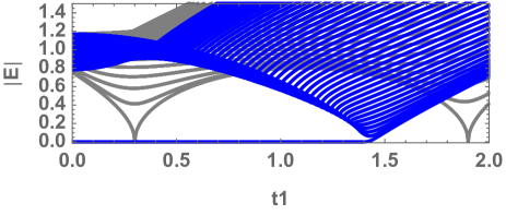
Figure 1: A typical energy spectrum of the non-hermitian SSH model [see Eq. (6)] under open boundary. The absolute value $|E|$ of the complex energy spectrum is shown in blue with varying $t_{1}$. Other parameters are $t_{2}=1$, $t_{3}=1/10$, $\gamma_{1}=3/4$, $\gamma_{2}=1/20$. The spectrum is obtained by numerically diagonalizing $H_{obc}$ at $2L=100$. For comparison, the spectrum of the same model under periodic boundary is shown in gray.

Terminologies such as bulk and edge geometries are convenient in considering topological systems. In hermitian systems, applying an open (periodic) boundary condition is equivalent to placing it in the edge (bulk) geometry. A quantum system is called topological when it exhibits protected gapless (or zero-energy) edge states in the edge geometry $g_{edge}$, while the corresponding topological number is defined in the bulk geometry $g_{bulk}$. Bulk-edge correspondence assures a one-to-one relation between the system’s behavior under $g_{edge}$ and under $g_{bulk}$. In non-hermitian systems this fundamental principle becomes elusive, at least superficially. Hu and Hughes (2011); Esaki et al. (2011); Kunst et al. (2018); Xiong (2018); Herviou et al. (2019); Kunst and Dwivedi (2019); Gong et al. (2018) Examples are known in which the number and locations of gap closing (topological phase transition) differ under open and periodic boundary conditions (see Fig. 1), i.e., the system’s behavior under $g_{edge}$ is no longer constrained by that under $g_{bulk}$. Such a feature is typical to non-hermitian system with anisotropic hopping. The underlying reason is the non-hermitian skin effect which refers to the fact that under open boundary condition even the bulk wave function tends to be localized in the vicinity of an edge. Lee (2016); Yao and Wang (2018); Kunst et al. (2018) The key to recover the bulk-edge correspondence is to reconsider the setting of $g_{bulk}$; the boundary condition concretizing $g_{bulk}$ needs to be readjusted in the presence of non-hermitian skin effect.

The purpose of this paper is to promote the use of the boundary condition which we dub modified periodic boundary condition (mpbc). The mpbc is the most appropriate boundary condition for realizing $g_{bulk}$ in non-hermitian topological systems that exhibit non-hermitian skin effect. Our scenario is illustrated by applying mpbc to the analysis of a non-hermitian SSH model with anisotropic hopping. Yao and Wang (2018); Yokomizo and Murakami (2019) We apply the proof of the bulk-edge correspondence of Ref. Ryu and Hatsugai, 2002 to this model with the use of mpbc. Under mpbc a pair of topological winding numbers $w_{\pm}$ [see Eq. (23)] are introduced to characterize the system. Our mpbc contains a free parameter $b$. Therefore, $w_{\pm}$ are the functions not only of the original set of parameters $\tau=\{t_{\mu},\gamma_{\mu}\}$ ($\mu=1,2,3,\cdots$) [see, e.g., Eqs. (6),(7)], but also of $b$. By evaluating $w_{\pm}$, a finite region in the generalized parameter space $\tilde{\tau}=\{\tau,b\}$ is identified to be topologically nontrivial, which is also smoothly connected to the known topological insulator (TI) region in the hermitian limit. In the same phase diagram we have also identified in addition to ordinary insulator (OI) regions, new topological regions specific to non-hermitian systems that have no analog in the hermitian limit.

II The modified periodic boundary condition

In a non-hermitian system even the bulk wave function does not necessarily extend over the entire system. To illustrate this let us consider the following 1D tight-binding model with an anisotropic hopping $t\neq t^{\prime}$; the so-called Hatano-Nelson model Hatano and Nelson (1996, 1997) in the clean limit:

$$H_{1}^{obc}=\sum_{j=1}^{L}(t|j+1\rangle\langle j|+t^{\prime}|j\rangle\langle j+1|),$$ (1)

where $|j\rangle$ represents a state localized at the $j$th site. In Eq. (1) an open boundary condition (obc) is implicit, since hopping amplitude are truncated at $j=1$ and $j=L$. Under obc, the wave function of the system tends to be localized as

$$\psi_{j}\propto b^{j}\sin kj,$$ (2)

where $b=\sqrt{t/t^{\prime}}$, $k=n\pi/(L+1)$ with $n=1,2,\cdots,L$. Compared with the hermitian case: $t=t^{\prime}$, the wave function (2) is multiplied by a factor $b^{j}$. Such a behavior, referred to as non-hermitian skin effect, manifests under obc. The quantity $b$ measures the degree of amplification (attenuation) of the wave function due to non-hermitian skin effect.

To establish a bulk-edge correspondence the existence of a reference surfaceless geometry is mandatory.Ryu and Hatsugai (2002) A winding number insuring the emergence of a zero-energy edge state under obc is defined in this geometry. In hermitian systems this role is concretized by the periodic boundary condition (pbc). In non-hermitian systems the ordinary pbc sometimes fails to play the same role. Yao and Wang (2018); Kunst et al. (2018) The positions of gap closing is an important part of the topological information on the system. Fig. 1 shows that in this non-hermitian system such an information does not seem to be kept properly when the boundary condition is changed from open to periodic.

The difficulty of the ordinary pbc stems from the fact that it fails to take proper account of the non-hermitian skin effect. To overcome this difficulty, we propose to use the following boundary Hamiltonian:

$$\Delta H_{1}^{mpbc}=b^{-L}t|1\rangle\langle L|+b^{L}t|L\rangle\langle 1|,$$ (3)

which represents a modified periodic boundary condition (mpbc) [as for the naming see text after Eq. (5)]. The matrix elements of Eq. (3) are to be added to the obc Hamiltonian (1). From an infinite set of fundamental solutions,

$$|\beta\rangle=\sum_{j}\beta^{j}|j\rangle,$$ (4)

of the infinite system, the factor $b^{\pm L}$ filters out those satisfying $|\beta|=b$, which mimic in a controllable manner the spatial amplification or attenuation of the wave function (2) under obc. Note that Eq. (3) is non-hermitian unless $b=1$.

The mpbc can be formulated on a more generic basis. To impose mpbc is equivalent to require

$$\psi(j+L)=b^{L}\psi(j),$$ (5)

to wave functions in an infinite system, in the sense that the resulting wave functions in any interval of $L$ sites are equivalent to those in the system of $L$ sites with mpbc. Note that such wave functions in the infinite system are not bounded and hence are not allowed in quantum mechanics, whereas those in the finite system have no such difficulty. Let $\psi_{j}$ be a wave functions that is selected by the condition (3). If one expresses this wave function as $\psi_{j}=b^{j}\phi_{j}$, then the rescaled wave function $\phi_{j}$ satisfies the ordinary periodic boundary condition: $\phi_{j+L}=\phi_{j}$, and in this sense the present boundary condition (3) may be called a modified periodic boundary condition.

To specify the mpbc (3), one has to specify the parameter $b$. In the simple model prescribed by Eq. (1), $b$ is uniquely determined as $b=\sqrt{t/t^{\prime}}$ to mimic the non-hermitian skin effect. However, in a more generic model, such a plausible value of $b$ generally depends on $k$ as each wave function exhibits its own spatial amplification or attenuation under obc. Taking these into account, below we consider $b$ as an independent parameter. This in turn signifies that the space of model parameters specifying our system has been slightly enlarged: $\tau\rightarrow\tilde{\tau}=\{\tau,b\}$. Later, we discuss the bulk-edge correspondence of our system in this generalized parameter space $\tilde{\tau}$.

III The model system

To illustrate our scenario we employ the SSH-type non-hermitian (tight-binding) Hamiltonians Lee (2016); Yao and Wang (2018); Lieu (2018) The nearest-neighbor (NN) SSH model with anisotropic hopping employed in Refs. Lee, 2016; Yao and Wang, 2018 gives a prototypical example in which one encounters the difficulty of applying the periodic boundary condition (pbc) to a non-hermitian system. Here, we consider a slightly generalized version of this model with third-nearest-neighbor (3NN) hopping: Yokomizo and Murakami (2019); Yao and Wang (2018)

$$H_{obc} = H_{\rm NN}+H_{\rm 3NN},$$ (6)

$$H_{\rm NN} = \sum_{j=1}^{L}\left[t_{1}^{-}|jB\rangle\langle jA|+t_{1}^{+}|jA\rangle\langle jB|\right]$$

$$+ \sum_{j=1}^{L-1}\left[t_{2}^{-}|j+1,A\rangle\langle j,B|+t_{2}^{+}|jB\rangle\langle j+1,A|\right],$$

$$H_{\rm 3NN} = \sum_{j=1}^{L-1}\left[t_{3}|j+1,B\rangle\langle jA|+t_{3}|jA\rangle\langle j+1,B|\right],$$

where

$$t_{1}^{\pm}=t_{1}\pm\gamma_{1},\ \ t_{2}^{\pm}=t_{2}\pm\gamma_{2},$$ (7)

represent intra- and inter-cell anisotropic hopping amplitudes. The total Hamiltonian $H_{obc}$ becomes hermitian in the limit: $\gamma_{1}=\gamma_{2}=0$. Note that the model parameters $t_{\mu}(\mu=1,2,3)$, $\gamma_{\mu}(\mu=1,2)$ are all real constants.

The open boundary condition (obc) is implicit in Eqs. (6), since hopping amplitudes are truncated at $j=1$ and $j=L$. The size of the system is $L$ in unit cells, and $2L$ in the number of sites. A typical energy spectrum of our model under open boundary is shown in Fig. 1 with varying $t_{1}$, while other parameters are $t_{2}=1$, $t_{3}=1/10$, $\gamma_{1}=3/4$, $\gamma_{2}=1/20$. The spectrum is obtained by numerically diagonalizing $H_{obc}$ at $2L=100$.

Now that our model is explicitly given, we can also write down the modified periodic boundary condition (mpbc) explicitly:

$$\Delta H_{\rm NN}^{mpbc} = b^{-L}t_{2}^{-}|1,A\rangle\langle L,B|+b^{L}t_{2}^{+}|L,B\rangle\langle 1,A|,$$

$$\Delta H_{\rm 3NN}^{mpbc} = b^{-L}t_{3}|1,B\rangle\langle L,A|+b^{L}t_{3}|L,A\rangle\langle 1,B|.$$ (8)

These boundary Hamiltonians are combined with the obc Hamiltonian $H_{obc}$ to give the mpbc Hamiltonian,

$$H_{mpbc}=H_{obc}+\Delta H_{\rm NN}^{mpbc}+\Delta H_{\rm 3NN}^{mpbc}.$$ (9)

The hopping matrix elements in Eqs. (8) connect the final unit cell $j=L$ back to the first one $j=1$, and vice versa. Note that the boundary Hamiltonians (8) are non-hermitian unless $b=1$.

In the following transformed basis,Hatano and Nelson (1996, 1997); Yao and Wang (2018) the mpbc (8) reduces to an ordinary pbc. Let $S$ be the transforming matrix:

$$S={\rm diag}[1,1,b,b,b^{2},b^{2},\cdots,b^{L-1},b^{L-1}],$$ (10)

and consider the similarity transformation:

$$\tilde{H}_{mpbc} = S^{-1}H_{mpbc}S$$

$$= \tilde{H}_{obc}+\Delta\tilde{H}_{\rm NN}^{mpbc}+\Delta\tilde{H}_{\rm 3NN}^{mpbc},$$

where $\tilde{H}_{obc}=\tilde{H}_{\rm NN}+\tilde{H}_{\rm 3NN}$ with

$$\tilde{H}_{\rm NN} = \sum_{j=1}^{L}\left[t_{1}^{-}|jB\rangle\langle jA|+t_{1}^{+}|jA\rangle\langle jB|\right]$$

$$+ \sum_{j=1}^{L-1}\left[b^{-1}t_{2}^{-}|j+1,A\rangle\langle j,B|+bt_{2}^{+}|jB\rangle\langle j+1,A|\right],$$

$$\tilde{H}_{\rm 3NN} = \sum_{j=1}^{L-1}\left[b^{-1}t_{3}|j+1,B\rangle\langle jA|+bt_{3}|jA\rangle\langle j+1,B|\right],$$

and

$$\Delta\tilde{H}_{\rm NN}^{mpbc} = b^{-1}t_{2}^{-}|1,A\rangle\langle L,B|+bt_{2}^{+}|L,B\rangle\langle 1,A|,$$

$$\Delta\tilde{H}_{\rm 3NN}^{mpbc} = b^{-1}t_{3}|1,B\rangle\langle L,A|+bt_{3}|L,A\rangle\langle 1,B|.$$ (12)

Note that $\Delta\tilde{H}_{\rm NN}^{mpbc}+\Delta\tilde{H}_{\rm 3NN}^{mpbc}$ represents the ordinary pbc for $\tilde{H}_{obc}$. In Sec. II we have seen that under (3) the rescaled wave function $\phi_{j}$ satisfies the ordinary pbc. Here, by a similarity transformation (III) the boundary Hamiltonians (8) representing the mpbc are reduced to the ones representing the ordinary pbc. These give us a good reason to call our boundary condition (8) modified pbc. Note that the similarity transformation (III) keeps the eigenvalues unchanged.

(a)
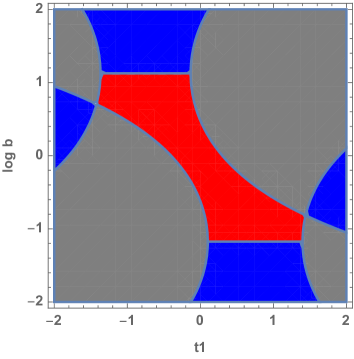
(b)

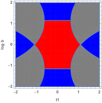
Figure 2: The phase diagrams in the space of parameters $(t_{1},b)$ determined by the winding number $w(t_{1},b)$ for (a) the non-hermitian case of $\gamma_{1}=3/4$, $\gamma_{2}=1/20$ and (b) the hermitian case of $\gamma_{1}=\gamma_{2}=0$. Other parameters are $t_{2}=1$, $t_{3}=1/10$. The regions of $w=1$ and $w=0$ are respectively painted in red and blue. The remaining gray area corresponds to $w=1/2$.

IV Generalized bulk-edge correspondence

For a hermitian system with chiral (sublattice Kawabata et al. (2018)) symmetry a clear proof of the bulk-edge correspondence is available.Ryu and Hatsugai (2002) In this proof the Hamiltonian $H(g_{bulk})$ in a reference bulk (closed, surfaceless) geometry $g_{bulk}$ is specified by a set of parameters, which correspond to $R_{\pm}$ in the following formulation. The role of $g_{bulk}$ is played by the ordinary periodic boundary condition (pbc) so that $H(g_{bulk})$ becomes the standard Bloch Hamiltonian $H(k)$, which is specified by $R_{+}(k)=R_{-}^{*}(k)=R(k)$. As $k$ sweeps the entire Brillouin zone, the trajectory of $R(k)$ forms a loop on this complex parameter plane. The topological property of $H(k)$ is encoded in the winding property of this loop with respect to the origin (a reference point). To judge whether the system is topologically trivial or not, one attempts to deform this loop continuously into a special one (e.g., to the one corresponding to $t_{1}=0$, $t_{2}=1$ and $t_{3}=0$), at which the existence of a zero-energy edge state is apparent in the edge geometry $g_{edge}$, i.e., under the open boundary condition (obc). The point is that to establish a bulk-edge correspondence, in addition to $g_{edge}$, the existence of $g_{bulk}$ is mandatory, and $g_{edge}$ is realized by a simple truncation of $g_{bulk}$ in real space. In non-hermitian systems ordinary pbc is no longer qualified for such a reference geometry, since it is incapable of capturing the nature of wave function that tends to amplify exponentially under obc. Introduction of ordinary pbc changes the nature of the wave function so abruptly that it even changes the topological nature of the system as indicated in Fig. 1.

Here, we show that the modified periodic boundary condition (mpbc) introduced in the last section provides with such a reference geometry for a generic non-hermitian topological system. Below, we show that the proof of bulk-edge correspondence as given in Ref. Ryu and Hatsugai, 2002 can be safely applied to a generic non-hermitian topological system, using the reference geometry specified by mpbc.

In parallel with the single-band case (see Sec. II) the eigenstate of $H_{mpbc}$ satisfying

$$H_{mpbc}|\beta\rangle=E(\beta)|\beta\rangle,$$ (13)

takes the following form:

$$|\beta\rangle=\sum_{j=1}^{L}\beta^{j}(c_{A}|jA\rangle+c_{B}|jB\rangle),$$ (14)

where

$$\beta=be^{ik},$$ (15)

with $k$ being real and in the range of the Brillouin zone: $k\in[0,2\pi]$. The coefficients $c_{A}$ and $c_{B}$ in Eq. (14) are determined by the eigenvalue equation:

$$H_{mpbc}(\beta)\left[\begin{array}[]{c}c_{A}\\ c_{B}\end{array}\right]=E(\beta)\left[\begin{array}[]{c}c_{A}\\ c_{B}\end{array}\right],$$ (20)

where

$$H_{mpbc}(\beta)=\left[\begin{array}[]{cc}0&R_{+}(\beta)\\ R_{-}(\beta)&0\end{array}\right]$$ (21)

is our reference bulk Hamiltonian, which is also explicitly chiral (sublattice Kawabata et al. (2018)) symmetric, and

$$R_{+}(\beta) = t_{1}^{+}+t_{2}^{-}\beta^{-1}+t_{3}\beta,$$

$$R_{-}(\beta) = t_{1}^{-}+t_{2}^{+}\beta+t_{3}\beta^{-1}.$$ (22)

Then, following Ref. Ryu and Hatsugai, 2002, let us introduce the winding numbers:

$$w_{\pm} = {1\over 2\pi}[\arg R_{\pm}(\beta)]_{k=0}^{2\pi}$$ (23)

$$= {1\over 2\pi}[\phi_{\pm}(2\pi)-\phi_{\pm}(0)],$$

where

$$\phi_{\pm}(k)={\rm Im}\log R_{\pm}(\beta),$$ (24)

with the choice of the branch of $\log$ such that $\phi_{\pm}(k)$ is continuous for $k\in[0,2\pi]$. As $k$ sweeps the entire Brillouin zone at a fixed $b$, the winding number $w_{\pm}$ measures how many times the trajectory of $\rho=R_{\pm}(\beta=be^{ik})$ encircles the origin in the complex $\rho$-plane in the anti-clockwise direction. The winding number such as the ones in Eq. (23) is widely used for characterizing a hermitian model of class AIII, e.g., the SSH model. Asbóth et al. (2015)

Fig. 2 (a) shows the phase diagram in the parameter space $(t_{1},b)$ determined by the winding numbers, $(w_{+},w_{-})$. The parameter space $(t_{1},b)$ represents a subspace of $\tilde{\tau}=\{\tau,b\}$ at which other model parameters are fixed to the following values: $t_{2}=1$, $t_{3}=1/10$, $\gamma_{1}=3/4$, $\gamma_{2}=1/20$. Here, to make the phase diagram look simpler, we employ the symmetric version of $w_{\pm}$ defined as

$$w=-{w_{+}-w_{-}\over 2}.$$ (25)

In the hermitian limit the hermiticity requires $R_{-}=R_{+}^{*}$, so that $w_{-}$ is fixed to $-w_{+}$. Therefore, $w=-w_{+}=w_{-}$; i.e., the symmetrization is not indispensable.

In Fig. 2 (a) painted in red is the region of $w=1$, corresponding to $(w_{+},w_{-})=(1,-1)$. Painted in blue is the region of $w=0$, corresponding to $(w_{+},w_{-})=(0,0)$. The remaining gray area corresponds to $w=1/2$, representing the regions of either $(w_{+},w_{-})=(1,0)$ or $(0,-1)$. In non-hermitian systems, $w_{+}$ and $w_{-}$ vary independently, taking in principle any combination of integral values. As a result, the symmetric winding number (25) can take half-integral values. Fig. 2 (b) shows a similar phase diagram in the limit: $\gamma_{1}=\gamma_{2}=0$. The regions of $w=1/2$ remains to exist even in this limit provided $b\neq 1$, while they disappear at $b=1$.

(a)
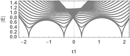
(b)
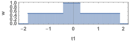
(c)
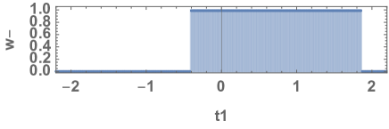
(d)

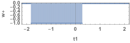
Figure 3: The spectrum and winding numbers under pbc. In (a), $|E|$ is plotted as a function of $t_{1}$. In (b)-(d), $w(t_{1},b=1)$ and $w_{\pm}(t_{1},b=1)$ are shown in the same parameter range. Parameters other than $t_{1}$ and $b$ are same as those in Fig. 1.

Let us argue that the two phase diagrams, the one at a generic value of $\gamma_{1}$ and $\gamma_{2}$ represented by Fig. 2 (a) and the one at $\gamma_{1}=\gamma_{2}=0$, are smoothly connected. On the phase boundaries of different topological phases at a generic value of $\gamma_{1}$ and $\gamma_{2}$ [Fig. 2 (a)] either of $\rho=R_{\pm}(\beta)$ touches the origin in the complex $\rho$-plane; i.e., either of

$$0 = |R_{-}(\beta)|=|t_{1}-\gamma_{1}+(t_{2}+\gamma_{2})\beta+t_{3}\beta^{-1}|,$$

$$0 = |R_{+}(\beta)|=|t_{1}+\gamma_{1}+(t_{2}-\gamma_{2})\beta^{-1}+t_{3}\beta|,$$ (26)

holds. As the non-hermitian parameters $\gamma_{1},\gamma_{2}$ vary, these phase boundaries deform smoothly, and in the limit of $\gamma_{1}=\gamma_{2}=0$, Eqs. (26) reduce to

$$0 = |R_{-}(\beta)|=|t_{1}+t_{2}\beta+t_{3}\beta^{-1}|,$$

$$0 = |R_{+}(\beta)|=|t_{1}+t_{2}\beta^{-1}+t_{3}\beta|.$$ (27)

These conditions indeed define the phase boundaries of different topological phases at $\gamma_{1}=\gamma_{2}=0$ [Fig. 2 (b)]. Since the phase boundaries are smoothly connected, topological phases enclosed by such phase boundaries are also smoothly connected.

Let us focus on a line of $b=1$ in the phase diagram at $\gamma_{1}=\gamma_{2}=0$ shown in panel (b). On this line, which we call $\eta_{0}$, the correspondence between the bulk winding number $w$ defined in $g_{bulk}$ and the existence/absence of a zero-energy edge state under $g_{edge}$ is well established; $w=1$ corresponds to the existence and $w=0$ to the absence of an edge state in $g_{edge}$. Ryu and Hatsugai (2002)

Let us consider a more generic path $\eta$ on the phase diagram shown in panel (a). Thanks to the smooth deformation described in the last paragraph, on any path $\eta$ smoothly connected to $\eta_{0}$, the correspondence in the behavior of the system under $g_{bulk}$ and the one under $g_{edge}$ is guaranteed. In Fig. 2(a) the central $w=1$ region is in contact with the right $w=0$ region by a single point $P$ located at $(t_{1},\log b)\simeq(1.44,-0.82)\equiv(t_{1c},\log b_{c})$. For the path $\eta$ to be smoothly connected to $\eta_{0}$, it must stay in the $w=1$ region until $t_{1}=t_{1c}$, then the path must go through the point $P$ to enter directly the right $w=0$ region. A similar argument applies on the $t_{1}<0$ side. Any of such a path $\eta$ is smoothly connected to $\eta_{0}$, and the corresponding bulk geometry $g_{bulk}$ is eligible for establishing the bulk-edge correspondence.

The bulk-edge correspondence in the hermitian limit is based on the smooth deformation of a loop $\rho=R_{-}(\beta=e^{ik})$ ($k\in[0,2\pi]$) in the space of model parameters $\tau$.Ryu and Hatsugai (2002) Here, in the non-hermitian case the same deformation must be done in the generalized parameter space $\tilde{\tau}=\{\tau,b\}$. In this sense the bulk-edge correspondence for non-hermitian topological systems is a generalized one.

The generalized bulk-edge correspondence just proven gives also a clear interpretation to the pbc spectrum shown in Fig. 1 at the back of the obc spectrum for comparison; recall that the number and locations of the gap closing are different in the two spectra. In Fig. 3 (a) the same pbc spectrum is plotted in a broader range of $t_{1}$. In panel (b) $w(t_{1},b=1)$ is plotted. With increasing $t_{1}$ from the left end, $w(t_{1},b=1)$ changes as $0\rightarrow 1/2\rightarrow 1\rightarrow 1/2\rightarrow 0$. This corresponds to the $b=1$ line in Fig. 2 (a). Each time $w(t_{1},b)$ changes, the pair of winding numbers $(w_{+},w_{-})$ changes, and hence the system undergoes a topological phase transition. A gap closing must occur at corresponding values of $t_{1}$. In panel (a), the central region around $t_{1}=0$ bounded by two gap closings at $t_{1}\simeq 0.3$ and at $t_{1}\simeq-0.4$ falls on the $w=1$ region. This is actually the part, which is smoothly connected to the TI phase under obc with a pair of zero-energy edge state. The two far ends of the spectrum ($t_{1}\lesssim-1.8,t_{1}\gtrsim 1.9$) correspond to the OI phase. The remaining intermediate region between the inner and outer gap closings falls on the new topological phase with $w=1/2$. Such a phase corresponding to $(w_{+},w_{-})=(1,0)$ or $(0,-1)$ has no analogue in the hermitian limit, realizing a new topologically distinct phase which is truly non-hermitian. Since these $w=1/2$ regions cannot be smoothly connected to a known topological phase in the hermitian limit (characterized by edge states under obc), we cannot characterize them in such a conventional way. We leave further analysis on the nature of these new topological phases to future study.

Strictly speaking, the proof given here is applicable to topological phases in the perturbative non-hermitian regime; to those connected smoothly to the corresponding hermitian topological phase. A more general proof of the bulk-edge correspondence valid also in the non-perturbative non-hermitian regime will be given elsewhere.

Unlike our recipe employing mpbc for $g_{bulk}$ and obc for $g_{edge}$ to recover the bulk-edge correspondence, the authors of Refs. Yao and Wang, 2018; Yokomizo and Murakami, 2019 developed an alternative approach employing only $g_{edge}$ specified by obc. Yao and Wang (2018); Yokomizo and Murakami (2019) Under mpbc the eigenstates of the system takes the generalized Bloch form (14). Under obc the eigenstate is no longer in this form; instead it becomes a linear combination of the Bloch form (14) with different $\beta$.Yokomizo and Murakami (2019) Ref. Yokomizo and Murakami, 2019 gives a recipe to find the bulk solutions compatible with obc in the limit of $L\rightarrow\infty$, where $|\beta|$ is not a constant but a function of $k$. The Brillouin zone, i.e., the trajectory $C_{\beta}$ of $\beta$, is no longer circular and has cusps in certain cases. Yao and Wang (2018); Yokomizo and Murakami (2019)

As for the bulk-edge correspondence, a winding number formally similar to the ones in Eq. (23) is employed to characterize the mapping from $C_{\beta}$ to a loop of $\rho=R_{\pm}(\beta)$. Yao and Wang (2018); Yokomizo and Murakami (2019) There, the integral over $k\in[0,2\pi]$ is replaced with a contour integral along $C_{\beta}$. In the derivation of these winding numbers, left and right eigenstates of the Bloch Hamiltonian $H(\beta)$ is needed. However, such left and right eigenstates are specified by a single $\beta$, so that they do not satisfy obc, while the values of $\beta$ on the contour $C_{\beta}$ result from obc. Recall that under obc the eigenstates are not in the form of (14). In this regard, our formulation is more natural as every procedure is carried out based on the mpbc (8). Furthermore, unlike the arguments of Refs. Yao and Wang, 2018; Yokomizo and Murakami, 2019, we start with a system of finite size $L$ then take safely the limit of $L\rightarrow\infty$ at the end of the formulation, as one usually does in the hermitian case.

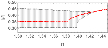
Figure 4: $|\beta(E_{bot})|$ is plotted in red as a function of $t_{1}$ in the vicinity of the phase transition at $t_{1}=t_{1c}\simeq 1.44$. Gray bars outline the region of $w=1$, which has already appeared in Fig. 2 (a) though here the vertical axis is in linear scale.

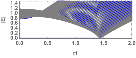
Figure 5: Spectrum under mpbc. $|E|$ is plotted in gray as a function of $t_{1}$. For comparison, the spectrum under obc (Fig. 1) is also plotted in blue. The plot is done in a system of size $2L=200$ for mpbc, while $2L=100$ for obc.

V Bulk-edge correspondence on an optimal path $\bar{\eta}$

Suppose that a path $\eta$ given on the $(t_{1},b)$-plane in Fig. 2(a) is smoothly connected to its hermitian counterpart $\eta_{0}$. This guarantees the bulk-edge correspondence between $g_{bulk}$ under mpbc with $\eta$ and $g_{edge}$ under obc as discussed in Sec IV. In the viewpoint of spectrum, the bulk-edge correspondence only ensures that the positions of the gap closing in $g_{bulk}$ are identical with those in $g_{edge}$. It is not mandatory that the mpbc spectrum on $\eta$ reproduces the bulk part of the obc spectrum completely.

Still it will not be useless to consider the optimal path $\bar{\eta}$, among an infinite number of possible paths, chosen such that the mpbc spectrum on $\bar{\eta}$ reproduces the bottom of the energy band in the bulk spectrum under obc. Since the gap closing is a property of the band bottom, this ensures that the positions of the gap closing are also reproduced. Despite that $\bar{\eta}$ is not the only but a possible choice of $\eta$, $\bar{\eta}$ has an advantage that it eases to follow the evolution of the spectrum from the one under $g_{bulk}$ to the one under $g_{edge}$. This is the simplest and most direct way to establish the bulk-edge correspondence.

In determining $\bar{\eta}$, note that the trajectory $C_{\beta}$ of $\beta$ defines the bulk energy band of $|E|\in[E_{bot},E_{top}]$ under obc, Yokomizo and Murakami (2019) indicating that $\beta$ should be regarded as a function of $E$. To reproduce the spectrum at the band bottom $E_{bot}$ under obc, we need to tune the parameter $b$ to be consistent with the value of $\beta$ corresponding to $E_{bot}$ at each $t_{1}$. Thus, $b$ should be determined as

$$b=|\beta(E_{bot})|.$$ (28)

As $\beta(E_{bot})$ varies as a function of $t_{1}$, $b$ determined as Eq. (28) defines a path $\bar{\eta}$ in the parameter space $(t_{1},b)$.

The path $\bar{\eta}$ defined in this way is smoothly connected to the one in the hermitian limit $\eta_{0}$. Fig. 4 shows the value of $|\beta(E_{bot})|$ against the $w=1$ region in the $(t_{1},b)$-space. It shows that within the accuracy of the numerical computation the value of $|\beta(E_{bot})|$ is always found in the $w=1$ region until the very end of this region $P$ located at $(t_{1},b)=(t_{1c},b_{c})$. After passing through the point $P$ the path $\bar{\eta}$ specified as $b=|\beta(E_{bot})|$ gets directly into the $w=0$ region (not shown).

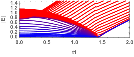
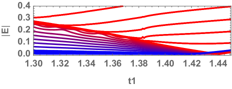
Figure 6: Evolution of the spectrum from mpbc to obc. $|E|$ is plotted as a function of $t_{1}$ at $2L=100$. The mpbc (8) with $b=|\beta(E_{bot})|$ is employed and then gradually switched off [$\delta$ in Eq. (29) varies from 1 to 0]. At $\delta$ away from the mpbc value ($\delta=1$) only data from the bottom of the spectrum is kept and added to the spectrum under mpbc (Fig. 5) in a color that varies continuously from red (mpbc) to blue (obc). Bottom: A detailed plot of the top panel in the vicinity of the phase transition ($t_{1}=t_{1c}$).

Fig. 5 shows the spectrum under mpbc with $b=|\beta(E_{bot})|$. At sight it looks reproducing the bulk part of the obc spectrum fairly well. Strictly speaking, the value of $|\beta(E_{bot})|$ is justified only in the $L\rightarrow\infty$ limit, while the obc spectrum is calculated at a finite $L$ ($2L=100$), so that this agreement is approximate. Also if one examines the spectrum more closely, one can recognize that the agreement is limited to the vicinity of the band bottom. But still, such an agreement is advantageous for making the bulk-edge correspondence intuitively accessible.

Assuming that the mpbc (8) with $b$ as given in Eq. (28) is initially imposed, let us gradually switch it off:

$$H_{\delta}=H_{obc}+\delta\left[H_{\rm NN}^{mpbc}+H_{\rm 3NN}^{mpbc}\right]_{b=|\beta(E_{bot})|}$$ (29)

with $\delta$ varied from 1 to 0. In Fig. 6 one can clearly see that a branch of spectrum detached from the bottom of the energy band in the purely bulk mpbc spectrum (situation of Fig. 5 at $\delta=1$) evolves continuously into the zero-energy edge state at obc ($\delta=0$). The smooth evolution is highlighted by a continuous change of plot colors used for that branch. This intuitive form of bulk-edge correspondence is first made possible thanks to mpbc.

VI Concluding remarks

The non-hermitian skin effect is specific to non-hermitian systems under open boundary conditions (obc). Under obc the wave function exhibits a typical exponential dependence and is localized near the boundary of the system. This non-hermitian skin effect is influential even to the topological nature of the system. The gap closing specifying the phase boundary between TI and OI phases under obc becomes unrecognizable in the spectrum under ordinary periodic boundary condition (pbc). The apparent failure of the bulk-edge correspondence in the ordinary pbc stems from the fact that it is incompatible with the skin effect.

Here, we have proposed a modified periodic boundary condition (mpbc), which takes a proper account of this effect in a closed geometry. The mpbc maintains the topological features that arise under obc, while the remnant of the skin effect can be clearly seen in the eigenfunctions under mpbc in spite of the closed geometry.

In the mpbc the non-hermitian skin effect is taken into account through a parameter $b$ that specifies the boundary condition. The correspondence between bulk and edge has been established in a generalized parameter space $\tilde{\tau}=\{\tau,b\}$, where $\tau$ is the space of model parameters. In this sense the concept of bulk-edge correspondence is generalized in non-hermitian systems. Following the arguments of Ref. Ryu and Hatsugai, 2002, we have proven this generalized bulk-edge correspondence, which constitutes the main result of the paper. The mpbc also enables us to conceive the idea of bulk-edge correspondence in a generic non-hermitian system intuitively as an evolution of the spectrum in the course of the continuous change of the boundary condition from mpbc to obc.