Ultralight dark photon as a model for early universe dark matter

Abstract

Dark photon is a massive vector field which interacts only with the physical photon through the kinetic mixing. This coupling is assumed to be weak so that the dark photon becomes almost unobservable in processes with elementary particles, but can serve as a dark matter particle. We argue that in very early Universe ($z>3000$) this vector field may have the equation of state of radiation ($w=1/3$) but later behaves as cold dark matter ($w=0$). This may slightly change the expansion rate of the Universe at early time and reduce the value of the sound horizon of baryon acoustic oscillations (standard ruler). As a result, in this model the value of the Hubble constant appears to be larger than that in the standard $\Lambda$CDM model. In particular, it is sufficient to have the dark photon mass of order $m\sim 10^{-27}-10^{-25}$ eV to fit the value of the Hubble constant to $H_{0}=73$ km s^-1Mpc^-1 thus resolving the Hubble tension.

I Introduction

The $\Lambda$CDM cosmological model, in spite of its simplicity, is very successful in describing the Universe expansion history. Recent measurements of the cosmic microwave background anisotropy Plank specify the parameters of the $\Lambda$CDM model with a very high precision. In particular, the inferred value of the Hubble constant is $H_{0}=67.4\pm 0.5$ km s^-1Mpc^-1, which, however, disagrees with the results from supernovae NS-Hubble ; NS-Hubble1 and lensing time delays Bonvin:2016crt ; Birrer:2018vtm . The latter experiments measure a greater value for $H_{0}$ of about $73$ km s^-1Mpc^-1. This discrepancy, known also as the “Hubble tension,” may indicate that the standard $\Lambda$CDM model is incomplete and requires some modifications.

As discussed in NS-Hubble , one of the possible resolutions of the Hubble tension is based on the assumption that at the early stage of the Universe’s expansion (during the radiation dominated epoch) there might be extra relativistic particle species which contributed to the radiation density. Such particles could be sterile neutrinos or any other light particles not accounted within the Standard Model of elementary particles. With these extra contributions to the radiation density, the expansion rate of the Universe would be larger, and the recombination epoch would start earlier. This reduces the value of the sound horizon for baryon acoustic oscillations (BAO) and, thus, dictates a larger value for $H_{0}$.

Following the above idea, it is natural to assume that in the early Universe there were extra vector fields, different from the visible photon field, which might contribute to the radiation density in the pre-recombination epoch. As they are unobservable now, these vector fields must interact very weakly with the visible matter and should have a small mass to describe stable particles. In particular, the so-called dark photon field which was introduced originally in DP1 ; DP2 as a model of dark matter particles may play this role. However, we will consider a general massive vector field which is not necessarily identified with the dark photon.

In this paper we present a solution of equations of motion of the massive vector field in the radiation dominated expanding Universe which behaves as radiation before certain time, but then changes to the cold dark matter state. Using this solution, we propose a modification of the standard $\Lambda$CDM model in which some fraction of the dark matter is composed of the massive vector fields. We then show that it is possible to fit the parameters of this model such that the value of the sound horizon is reduced by about 6%, and the inferred value of the Hubble constant becomes $73$ km s^-1Mpc^-1.

As was demonstrated in recent publications Poulin:2018cxd ; Poulin:2018dzj , a similar result may be achieved with the use of a scalar field, which may be identified with the axion-like particles. The model presented in these papers, however, is based on a modification of the equation of state of the dark energy at early time while in this paper we propose to modify the equation of state of dark matter. Indeed, the equation of state of a “frozen” scalar field is equivalent to the cosmological constant which plays minor role at early Universe. A useful feature of the vector field model considered in this paper is that the vector field automatically behaves as radiation in early Universe even for the simplest model of the massive vector field minimally coupled to gravity, but after some critical time (which is equal to the inverse mass of the vector field) it turns to the state of cold dark matter. Therefore, our model represents an extension of the $\Lambda$CDM model such that some (small) fraction of the dark matter is “hot” during a short period of time in early Universe.

One of the typical issues with vector fields in cosmology is that any particular vector field solution may create a preferred direction and break the isotropy of the Universe. The isotropy of the Universe may be preserved in one of the two ways: (i) with the use of a triplet of mutually orthogonal vector fields with the same mass and the same magnitude or (ii) by considering a large number of randomly oriented vector fields. As was demonstrated within the vector inflation model Mukhanov , the latter model predicts a small anisotropy of the Universe while the triplet model provides fully isotropic solution. Although both cases are interesting, in this paper we will focus only on the triplet model which exactly preserves the isotropy of the Universe.

One may also question about mechanisms of production of the vector fields in early Universe. As was shown in Graham , ultra-light vector fields may be generated from inflationary fluctuations in a sufficient abundance to model the dark matter. Although the authors of Graham considered the vector fields with the mass $m\gtrsim 10^{-5}$ eV, they did not exclude the scenario that some fraction of the dark matter might be described by much lighter vector fields homogeneous in space. Note also that alternative scenarios of generating relic massive vector fields were proposed in Refs. 1 ; 2 ; 3 .

The rest of this paper is organized as follows. In section II we consider a solution of the massive vector field in the radiation-dominated expanding Universe and study the equation of state corresponding to this solution. In section III we use the obtained solution to modify the standard $\Lambda$CDM model so that at early time of the Universe’s expansion there is an excess of radiation density which slightly changes the expansion rate and the Hubble constant. The last section is devoted to a discussion of the presented model.

II Massive vector field in expanding Universe

We start this section by briefly revisiting the massive vector field model in the expanding Universe with the focus on the equation of state of this field in the spatially homogeneous case. We then consider a particular solution of the equation of motion for this field corresponding to the radiation-dominated epoch.

II.1 Homogeneous massive vector field in expanding Universe

Let us consider a homogeneous and isotropic expanding Universe with the metric $g_{\mu\nu}={\rm diag}(-1,a^{2},a^{2},a^{2})$, where $a=a(t)$ is the scale factor. The Lagrangian of a massive vector field $A_{\mu}$ on this background reads

$$L=\sqrt{-g}\left(-\frac{1}{4}F_{\mu\nu}F^{\mu\nu}-\frac{m^{2}}{2}A^{\mu}A_{\mu}\right)\,,$$ (1)

where $F_{\mu\nu}=\partial_{\mu}A_{\nu}-\partial_{\nu}A_{\mu}$ and $g=\det g_{\mu\nu}=-a^{6}$. The corresponding equation of motion (Maxwell-Proca equation) reads

$$-\frac{1}{\sqrt{-g}}\partial_{\mu}\sqrt{-g}F^{\mu\nu}+m^{2}A^{\nu}=0\,.$$ (2)

The conserved stress-energy tensor has standard form

$$T_{\mu\nu}=F_{\mu\alpha}F_{\nu}{}^{\alpha}-\frac{1}{4}g_{\mu\nu}F_{\alpha\beta}F^{\alpha\beta}-\frac{m^{2}}{2}g_{\mu\nu}A_{\alpha}A^{\alpha}+m^{2}A_{\mu}A_{\nu}\,.$$ (3)

Let ${\bf A}$ and $\phi$ be 3+1 components of the vector field, $A_{\mu}=(-\phi,{\bf A})$, ${\bf A}\equiv(A_{i})=(A_{1},A_{2},A_{3})$. In terms of these components, the electric and magnetic fields may be defined as

$${\bf E}=-\dot{\bf A}-\nabla\phi\,,\quad{\bf B}=\nabla\times{\bf A}\,,$$ (4)

where the dot over the field stands for the time derivative, e.g., $\dot{\bf A}\equiv\partial_{t}{\bf A}$. In the non-covariant form, the equation of motion (2) reads

$$\nabla\cdot{\bf E}+m^{2}a^{2}\phi = 0\,,$$ (5a)

$$-\dot{\bf E}-\frac{\dot{a}}{a}{\bf E}+\frac{1}{a^{2}}\nabla\times{\bf B}+m^{2}{\bf A} = 0\,.$$ (5b)

We will look for a homogeneous solution of the equations (5), $\partial_{i}A_{\mu}=0$. In this case, Eq. (5a) implies $\phi=0$ and ${\bf A}={\bf A}(t)$, while Eq. (5b) reduces to

$$\ddot{\bf A}+\frac{\dot{a}}{a}\dot{\bf A}+m^{2}{\bf A}=0\,.$$ (6)

A solution of this equation gives homogeneous electric field with vanishing magnetic field, ${\bf B}=0$.

The 3+1 components of the stress-energy tensor (3) are

$$T_{00} = \frac{1}{2a^{2}}({\bf E}^{2}+m^{2}{\bf A}^{2})\,,$$ (7)

$$T_{ij} = -E_{i}E_{j}+\frac{1}{2}\delta_{ij}{\bf E}^{2}+m^{2}A_{i}A_{j}-\frac{m^{2}}{2}\delta_{ij}{\bf A}^{2}\,,$$ (8)

and $T_{0i}=0$ for the homogeneous vector field subject to Eq. (6). Note that the tensor $T_{ij}$ is non-diagonal since the electric field creates anisotropy of the Universe.

Since no anisotropy of the Universe is observed Plank , the stress-energy tensor (8) should have the diagonal form. The isotropy of the expanding Universe driven by vector fields may be naturally achieved in one of the two ways: (i) using a triplet of mutually orthogonal vector fields with the same mass and magnitude and (ii) by applying a large number $N$ of randomly oriented vector fields which have no preferred direction in average. In the latter case, as was demonstrated in the vector inflation model Mukhanov , the off-diagonal components of the stress-energy tensor are not exactly vanishing, but are proportional to $\sqrt{N}$ predicting a small anisotropy of the Universe. Although this case may be interesting, in this paper we will consider the fully isotropic vector field model based in the triplet of orthogonal vector fields.

Let $A^{(a)}_{\mu}$, $a=1,2,3$, be a triplet of mutually orthogonal vector fields with the same mass $m$ and magnitude $|{\bf A}|$. One can prove the following simple identities by averaging over the species: $\overline{A_{i}A_{j}}\equiv\frac{1}{3}\sum_{a}A^{(a)}_{i}A^{(a)}_{j}=\frac{1}{3}\delta_{ij}{\bf A}^{2}$, $\overline{E_{i}E_{j}}\equiv\frac{1}{3}\sum_{a}E^{(a)}_{i}E^{(a)}_{j}=\frac{1}{3}\delta_{ij}{\bf E}^{2}$. As a result, the tensor (8) in average acquires the diagonal form

$$\overline{T_{ij}}=\frac{1}{6}\delta_{ij}({\bf E}^{2}-m^{2}{\bf A}^{2})\,.$$ (9)

The equations (7) and (9) define the energy density $\rho=T^{00}$ and pressure $\overline{T_{i}^{j}}=p\delta_{i}^{j}$ created by the triplet of massive vector fields,

$$\rho = \frac{1}{2a^{2}}({\bf E}^{2}+m^{2}{\bf A}^{2})\,,$$ (10)

$$p = \frac{1}{6a^{2}}({\bf E}^{2}-m^{2}{\bf A}^{2})\,.$$ (11)

The corresponding equation of state reads

$$w\equiv\frac{p}{\rho}=\frac{1}{3}\frac{{\bf E}^{2}-m^{2}{\bf A}^{2}}{{\bf E}^{2}+m^{2}{\bf A}^{2}}\,.$$ (12)

In the massless case, $m=0$, this parameter corresponds to the equation of state of radiation, $w=\frac{1}{3}$, but for non-vanishing mass it changes in the interval $-\frac{1}{3}\leq w\leq\frac{1}{3}$.

Note also that Eq. (12) resembles the equation of state of the constant magnetic field solution in massive electrodynamics considered in Ryutov:2017oeq .

II.2 Massive vector field solution in early Universe

In the radiation-dominated epoch, the scale factor $a$ is well approximated by

$$a(t)=(2\sqrt{\Omega_{\rm r}}H_{0}t)^{1/2}\,,$$ (13)

where $\Omega_{\rm r}$ is the radiation density and $H_{0}$ is the Hubble constant. With this scale factor Eq. (6) reduces to

$$\ddot{\bf A}+\frac{1}{2t}\dot{\bf A}+m^{2}{\bf A}=0\,.$$ (14)

The general solution of this equation reads

$${\bf A}(t)={\bf A}_{0}\cdot(mt)^{\frac{1}{4}}\left(c_{1}J_{\frac{1}{4}}(mt)+c_{2}Y_{\frac{1}{4}}(mt)\right)\,,$$ (15)

where $J$ and $Y$ are the Bessel functions, ${\bf A}_{0}$ is a constant vector, and $c_{1}$, $c_{2}$ are the integration constants. The corresponding electric field is found from Eq. (4),

$${\bf E}(t)=-{\bf A}_{0}\cdot m(mt)^{\frac{1}{4}}\left(c_{1}J_{-\frac{3}{4}}(mt)+c_{2}Y_{-\frac{3}{4}}(mt)\right)\,.$$ (16)

For this solution, the energy density (10) reads

$$\rho = \frac{|{\bf A}_{0}|^{2}m^{2}\sqrt{mt}}{2a^{2}}\bigg{[}\left(c_{1}J_{-\frac{3}{4}}(mt)+c_{2}Y_{-\frac{3}{4}}(mt)\right)^{2}$$ (17)

$$+\left(c_{1}J_{\frac{1}{4}}(mt)+c_{2}Y_{\frac{1}{4}}(mt)\right)^{2}\bigg{]}\,.$$

The energy density (17) has the following asymptotics for $c_{1}+c_{2}\neq 0$:

$$\rho\approx|{\bf A}_{0}|^{2}\left\{\begin{array}[]{l}\frac{\sqrt{2}m(c_{1}+c_{2})^{2}}{\Gamma^{2}(\frac{1}{4})}\frac{1}{a^{2}t}\quad\mbox{ for }\quad mt\ll 1\\ 2m^{2}(c_{1}^{2}+c_{2}^{2})\frac{1}{a^{2}\sqrt{mt}}\quad\mbox{ for }\quad mt\gg 1\,.\end{array}\right.$$ (18)

Thus, taking into account Eq. (13), we conclude that the energy density of the homogeneous massive vector field in the early Universe scales as radiation for $t\ll m^{-1}$ and as cold dark matter for $t\gg m^{-1}$,

$$\rho\propto\left\{\begin{array}[]{l}a^{-4}\quad\mbox{ for }\quad t\ll m^{-1}\\ a^{-3}\quad\mbox{ for }\quad t\gg m^{-1}\,.\end{array}\right.$$ (19)

Therefore, the equation of state of this field may be approximated by the step function,

$$\bar{w}=\left\{\begin{array}[]{ll}\frac{1}{3}&\mbox{ for }t<m^{-1}\\ 0&\mbox{ for }t>m^{-1}\,.\end{array}\right.$$ (20)

The above solution is valid for arbitrary initial conditions except for $c_{1}+c_{2}=0$. In the latter case, for $mt\ll 1$ the energy density has the following asymptotics $\rho\approx\frac{m^{2}\Gamma^{2}(\frac{1}{4})}{\sqrt{2}\pi^{2}a^{2}}$ which corresponds to $w=-\frac{1}{3}$. We assume that this case is not realized in Nature since it requires special initial conditions.

We stress that the massive vector field solution (15) is not universal as it applies only in the radiation-dominated epoch. At later times, e.g., in the matter-dominated epoch, the behavior of the vector field may change, but its density should be negligible compared with the matter density (including the dark matter) to avoid significant changes in the expansion rate of the late Universe.

III Implication to the Hubble tension problem

For completeness of our presentation, we start this section with a short review of the standard $\Lambda$CDM model. We then present a modification of this model which may resolve the Hubble tension problem while keeping all other conclusions of this model intact.

III.1 $\Lambda$CDM model and the standard ruler

The Hubble parameter $H\equiv\frac{\dot{a}}{a}$ in the $\Lambda$CDM model is given by

$$H(a)\equiv H_{0}E(a)=H_{0}\sqrt{\Omega_{\rm r}a^{-4}+\Omega_{\rm m}a^{-3}+\Omega_{\Lambda}}\,,$$ (21)

where $H_{0}$ is the Hubble constant and $\Omega_{\rm r}$, $\Omega_{\rm m}$, and $\Omega_{\Lambda}$ are density parameters of the radiation, matter and cosmological constant, respectively. Here we consider the spatially flat Universe, for simplicity. Note that $\Omega_{\rm m}$ takes into account both baryonic and cold dark matter, $\Omega_{\rm m}=\Omega_{\rm b}+\Omega_{\rm c}$, while the radiation density is the sum of photon and neutrino contributions, $\Omega_{\rm r}=\Omega_{\gamma}+\Omega_{\nu}$. The values of these parameters can be taken from the Particle Data Group review PDG : $H_{0}=67.8$ km s^-1 Mpc^-1, $\Omega_{\rm b}=0.048$, $\Omega_{\rm c}=0.258$, $\Omega_{\gamma}=5.37\times 10^{-5}$, $\Omega_{\nu}=3.66\times 10^{-5}$, $\Omega_{\Lambda}=0.692$. Note that the density parameter $\Omega_{\nu}$ corresponds to relativistic neutrinos since we are going to apply Eq. (21) at early times of the Universe expansion.

The early Universe may be considered as a hot plasma composed mainly of baryons, electrons and photons. Density fluctuations in this plasma are known to propagate in the form of sound waves with the speed Ma:1995ey

$$c_{s}(a)=\frac{c}{\sqrt{3\left(1+\frac{3a\Omega_{\rm b}}{4\Omega_{\gamma}}\right)}}\,,$$ (22)

where $c$ is the speed of light. Such sound waves propagate until the decoupling of photons that occurs ar redshift $z_{*}\approx 1090$. As a result, initial perturbations generate spherical waves in the primordial plasma with the comoving sound horizon, which is also known as the “standard ruler,”

$$r_{s}=\frac{1}{H_{0}}\int_{0}^{a_{*}}\frac{c_{s}(a)da}{a^{2}E(a)}\,,$$ (23)

where $a_{*}=(z_{*}+1)^{-1}$. Direct numerical evaluation of this integral with the above given parameters of the $\Lambda$CDM model yields $r_{s}\approx 145$ Mpc. This estimate is in a good agreement with the WMAP CMB observations WMAP which constrain this parameter as $r_{s}=146.8\pm 1.8$ Mpc.

The BAO data allows one to consider the sound horizon as a standard comoving ruler, whose length is independent of redshift and orientation, but is not necessarily correlated with CMB data which fix the parameters of the $\Lambda$CDM model and the Hubble constant. As a result, BAO data may be used to impose the constraint on the product $(r_{s}\cdot H_{0})$ Aubourg :

$$\frac{c}{r_{s}H_{0}}=29.63^{+0.48}_{-0.45}\,,$$ (24)

where $c$ is the speed of light.

In what follows, we will consider an extension of the $\Lambda$CDM model which predicts a reduced value of the sound horizon $r_{s}$ and a larger value for $H_{0}$ according to the constraint (24). We will show that it is possible to fit the parameters of this model such that the predicted value of the Hubble constant agrees with the local measurements of this constant from cephidae and supernovae observations: $H_{0}=73.24\pm 1.74\mbox{ km s}^{-1}\mbox{Mpc}^{-1}$ NS-Hubble ; NS-Hubble1 .

III.2 Extension of the $\Lambda$CDM model

We will consider an extension of the $\Lambda$CDM model in which some fraction $\Omega_{A}$ of the dark matter is described by the massive vector field ${\bf A}$ subject to the equation (14). We assume that this field was produced non-thermally and was present as a relic after the inflation epoch. Assuming also that this field was produced homogeneously with the equation of state $w=\frac{1}{3}$ at the beginning of radiation-dominated epoch ($t=0$), its equation of state at later times may be approximately described by the function (20). This field contributes to the expansion rate of the Universe through the following modification of the Hubble parameter (21):

$$E(a)=\sqrt{\frac{\Omega_{\rm r}}{a^{4}}+\frac{\Omega_{\rm m}-\Omega_{A}}{a^{3}}+\frac{\Omega_{A}}{a^{3(w+1)}}+\Omega_{\Lambda}}\,.$$ (25)

Here we added the term with $\Omega_{A}$ which describes the massive vector field with the equation of state $w$ and reduced the matter density by the same amount in order to keep the balance $\Omega_{\rm r}+(\Omega_{\rm m}-\Omega_{A})+\Omega_{A}+\Omega_{\Lambda}=1$.

In this model, we have two free parameters: the energy density $\Omega_{A}$ and the mass of the vector field $m$ which enters the equation of state as in Eq. (17). Both these parameters are assumed to be small enough to provide minor violations from the standard $\Lambda$CDM model.

In the particular case, when the equation of state is approximated by Eq. (20), the Hubble function (25) may be written as

$$E(a)=\left\{\begin{array}[]{l}\sqrt{\frac{\Omega_{\rm r}+\Omega_{A}}{a^{4}}+\frac{\Omega_{\rm m}-\Omega_{A}}{a^{3}}+\Omega_{\Lambda}}\,,\quad mt<1\\ \sqrt{\Omega_{\rm r}a^{-4}+\Omega_{\rm m}a^{-3}+\Omega_{\Lambda}}\,,\quad mt>1\,.\end{array}\right.$$ (26)

This function shows that at early times ($t<m^{-1}$) the massive vector field behaves as the radiation and gives additional contributions to the radiation density, but it quickly changes its equation of state such that after the critical time $t=m^{-1}$ it behaves as cold dark matter. The extra contributions to the radiation density lead to the increase of the expansion rate of the Universe at early times and, thus, to changes of our estimates of the Hubble constant obtained within the extended $\Lambda$CDM model.

In the modified $\Lambda$CDM model with the Hubble function (26), the formula for the sound horizon (23) has the form

$$r_{s} = \frac{1}{H_{0}}\int_{0}^{a_{1}}\frac{c_{s}(a)da}{\sqrt{\Omega_{\rm r}+\Omega_{A}+(\Omega_{\rm m}-\Omega_{A})a+\Omega_{\Lambda}a^{2}}}$$ (27)

$$+\frac{1}{H_{0}}\int_{a_{1}}^{a_{*}}\frac{c_{s}(a)da}{\sqrt{\Omega_{\rm r}+\Omega_{\rm m}a+\Omega_{\Lambda}a^{2}}}\,,$$

where $a_{1}=\left(\frac{2\sqrt{\Omega_{\rm r}}H_{0}}{m}\right)^{\frac{1}{2}}$ and $a_{*}=1/1091$.

To perform numerical estimates, we have to make some assumptions about the value of the density parameter $\Omega_{A}$. This parameter should not be much smaller than the density of radiation; otherwise the effect of the massive vector field would be negligible in the evolution of the Universe, $0.1\Omega_{\rm r}\lesssim\Omega_{A}$. This parameter is also bounded from above by the requirement that the massive vector field should not change the expansion rate at the matter dominated epoch driven mainly by the dark matter, $\Omega_{A}\ll\Omega_{\rm c}$. More precisely, we require that $\Omega_{A}$ should be smaller than the uncertainty in the measurements of the dark matter density which is $\Omega_{\rm c}=0.258\pm 0.00435$ PDG . Therefore, we will consider the energy density parameter of the massive vector field in the interval

$$9.0\times 10^{-5}<\Omega_{A}<4.4\times 10^{-3}\,.$$ (28)

The mass parameter $m$ may be limited by the applicability of the considered solution (15). Since this solution holds only in the radiation-dominated epoch, we should apply it only for redshifts $z>3600$. When the Universe passes to the matter-dominated epoch, the equation of state of this solution (20) should change to the matter type. This constrains the mass of the vector field through the equation (13), $m>2\cdot 3600^{2}\sqrt{\Omega_{\rm r}}H_{0}$, or

$$m>3.6\times 10^{-28}\mbox{ eV}.$$ (29)

We can now use the relation (24) to find the value of the Hubble constant $H_{0}$ via the known value for the sound horizon $r_{s}$ obtained within the modified $\Lambda$CDM model. We find that the Hubble constant gets the value $H_{0}=73$ km s^-1 Mpc^-1 when the parameters $m$ and $\Omega_{A}$ lie within the shaded region on the graph in Fig. 1.

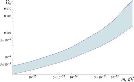
Figure 1: Allowed region for the parameters of mass $m$ and density $\Omega_{A}$ in the massive vector field model.

IV Conclusions

In this paper, we propose a modification of the standard $\Lambda$CDM model in which a (small) fraction of the dark matter is described by a massive vector field. We consider the general homogeneous solution of the equation of motion of this field in expanding Universe during the radiation dominated epoch. To preserve the isotropy of the Universe, we consider a triplet of mutually orthogonal fields with the same mass and magnitude. In this case, we show that the energy density of this solution behaves as radiation ($w=\frac{1}{3}$) during the time $t<m^{-1}$, but for $t>m^{-1}$ it changes to the cold dark matter ($\bar{w}=0$).

We consider an implication of the massive-vector-field extended $\Lambda$CDM model to resolve the Hubble tension. As was argued in NS-Hubble , this tension may be naturally resolved by increasing the number of relativistic particle species during the radiation-dominated epoch. Since the massive vector field behaves as radiation at early times, it may be naturally used to resolve this issue. We demonstrate that when the mass of the vector field is in the interval $10^{-27}-10^{-25}$ eV, and the energy density is of order $\Omega_{A}\sim 10^{-5}-10^{-2}$, the massive vector field slightly enhances the expansion rate of the Universe and reduces the sound horizon of baryon acoustic oscillation by about 6%. As a result, the inferred value of the Hubble constant appears to be 73 km s^-1Mpc^-1, which is in agreement with the results from supernovae NS-Hubble ; NS-Hubble1 and lensing time delays Bonvin:2016crt ; Birrer:2018vtm .

We stress that a similar result may be obtained with the use of a scalar axion-like field Poulin:2018cxd ; Poulin:2018dzj , which plays the role of dark energy with very specific equation of state. The main feature of the vector field model is that it corresponds to the modification of dark matter rather than the dark energy and automatically behaves as radiation at early times.

The massive vector field considered in this paper may be naturally identified with the so-called dark photon field introduced originally in DP1 ; DP2 and used in many subsequent publications as a model for dark matter. There are strict constraints on the parameters of this model (mass and coupling constant) from different experiments, see, e.g., DPrev1 ; DPrev2 ; DPrev3 ; DPrev4 ; DPmy . In this paper, however, we consider the ultralight massive vector field which is not necessary identified with the dark photon since we do not specify its interaction with visible matter. This interaction is assumed to be very weak to prevent the thermalization of the vector field in the early Universe plasma.

Acknowledgments

This work is supported by the Australian Research Council Grant No. DP150101405 and by a Gutenberg Fellowship.

References

- (1) N. Aghanim et al. [Planck Collaboration], arXiv:1807.06209 [astro-ph.CO].
- (2) A. G. Riess et al., Astrophys. J. 826, no.1, 56 (2016), arXiv:1604.01424 [astro-ph.CO].
- (3) A. G. Riess et al., Astrophys. J. 861, no. 2, 126 (2018), arXiv:1804.10655 [astro-ph.CO].
- (4) V. Bonvin et al., Mon. Not. Roy. Astron. Soc. 465, no. 4, 4914 (2017), arXiv:1607.01790 [astro-ph.CO].
- (5) S. Birrer et al., Mon. Not. Roy. Astron. Soc. 484, 4726 (2019), [arXiv:1809.01274 [astro-ph.CO]].
- (6) B. Holdom, Phys. Lett. B 166, 196 (1986).
- (7) P. Galison and A. Manohar, Phys. Lett. B 136, 279 (1984).
- (8) V. Poulin, T. L. Smith, T. Karwal and M. Kamionkowski, Phys. Rev. Lett. 122, no. 22, 221301 (2019), arXiv:1811.04083 [astro-ph.CO].
- (9) V. Poulin, T. L. Smith, D. Grin, T. Karwal and M. Kamionkowski, Phys. Rev. D 98, no. 8, 083525 (2018), arXiv:1806.10608 [astro-ph.CO].
- (10) A. Golovnev, V. Mukhanov and V. Vanchurin, JCAP 0806, 009 (2008), arXiv:0802.2068 [astro-ph].
- (11) P. W. Graham, J. Mardon and S. Rajendran, Phys. Rev. D 93, no. 10, 103520 (2016), arXiv:1504.02102 [hep-ph].
- (12) A. E. Nelson and J. Scholtz, Phys. Rev. D 84, 103501 (2011), arXiv:1105.2812 [hep-ph].
- (13) P. Arias, D. Cadamuro, M. Goodsell, J. Jaeckel, J. Redondo and A. Ringwald, JCAP 1206, 013 (2012), arXiv:1201.5902 [hep-ph].
- (14) K. Dimopoulos, Phys. Rev. D 74, 083502 (2006), hep-ph/0607229.
- (15) D. D. Ryutov, D. Budker and V. V. Flambaum, Astrophys. J. 871, no. 2, 218 (2019), arXiv:1708.09514 [astro-ph.GA].
- (16) M. Tanabashi et al. (Particle Data Group), Phys. Rev. D 98, 030001 (2018).
- (17) C. P. Ma and E. Bertschinger, Astrophys. J. 455, 7 (1995), astro-ph/9506072.
- (18) E. Komatsu et al. [WMAP Collaboration], Astrophys. J. Suppl. 180, 330 (2009), arXiv:0803.0547 [astro-ph].
- (19) É. Aubourg et al., Phys. Rev. D 92, no. 12, 123516 (2015), arXiv:1411.1074 [astro-ph.CO].
- (20) M. Raggi and V. Kozhuharov, Riv. Nuovo Cim. 38, no. 10, 449 (2015).
- (21) I. G. Irastorza and J. Redondo, Prog. Part. Nucl. Phys. 102, 89 (2018), arXiv:1801.08127 [hep-ph].
- (22) J. Jaeckel, Frascati Phys. Ser. 56, 172 (2012), arXiv:1303.1821 [hep-ph].
- (23) E. Arik et al. [CAST Collaboration], JCAP 0902, 008 (2009), arXiv:0810.4482 [hep-ex].
- (24) V. V. Flambaum, I. B. Samsonov and H. B. Tran Tan, Phys. Rev. D 99, no. 11, 115019 (2019), arXiv:1904.02271 [hep-ph].