A Note on Singularity Formation for a Nonlocal Transport Equation
Abstract
The -patch model is used to study aspects of fluid equations. We show that solutions of this model form singularities in finite time and give a characterization of the solution profile at the singular time.
1 Introduction
One of the most fundamental equations in modeling the motion of fluids and gases is the transport equation
| (1) |
here written using the vorticity . The velocity may depend on , in which case (1) is called an active scalar equation.
When the relationship is specified, (1) gives rise to many important models in fluid dynamics. is often called a Biot-Savart law. Here are some examples of particular transport equations, which are also active scalar equations. Take for example,
| (2) |
where is the perpendicular gradient. Equations (1) and (2) are the vorticity form of 2D Euler equations. As another example, one can take
Then (1) becomes the surface quasi-geostrophic (SQG) equation. The SQG equation has important applications in geophysics and atmospheric sciences Ped . Moreover it serves as a toy model for the 3D-Euler equations (see constantin1994formation for more details).
A question of great importance is whether solutions for these equations form singularities in finite time.
A game-changing observation in dealing with some two- and three dimensional models for fluid motion is that imposing certain symmetries on the solution of (1) on simple domains like a half-disc or a quadrant creates a special kind of flow called a hyperbolic flow. We will not go into details here but refer to Hoang2D ; HouLuo2 ; HouLuo3 ; kiselev2013small for more information. In this hyperbolic flow scenario, it seems that the behavior of the fluid on and near the domain boundary plays the most important part in creating either blowup or strong gradient growth. One-dimensional models capturing this behavior are therefore an essential tool for investigating possible blowup mechanisms without the additional complications of more-dimensional equations. We refer to sixAuthors for discussion of the aspects relating to the hyperbolic flow scenario. For 1d models of fluid equations, see also sixAuthors ; CKY ; CLM ; CCF .
In this paper, we will study a 1D model of (1) on with the following Biot-Savart law:
| (3) |
This model is called -patch model and has also been treated in dong2014one with an additional viscosity term causing dissipation. Local existence of the solution and the existence of a blowup for the viscous -patch model were given in dong2014one . The existence of blowup was obtained by using energy methods. In contrast, this paper deals with more geometric aspects of singularity formation for the inviscid model - such as the final profile of the solution at the singular time.
Regularity-wise, the -patch model is less regular than 1D Euler and more regular than the Córdoba-Córdoba-Fontelos (CCF) model (see CCF ). The latter is a 1D analogue of the SQG equation.
2 One dimensional -patch model and main results
We study the transport equation
| (4) |
in one space dimension for the unknown function with sufficiently smooth initial data . The velocity field is given by the nonlocal Biot-Savart law
| (5) |
The -patch model becomes the 1d model for the 2d Euler equation in the limit with velocity field given by
| (6) |
For convenience, we will assume the constant associated with the fractional Laplacian is , and we write .
We consider classical solutions where is odd in and such that
| (7) |
for all . Here, the norm is defined by
| (8) |
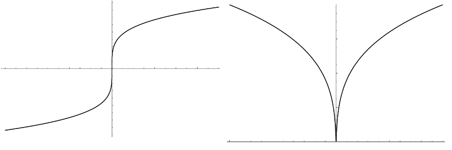
Our main concern will be the question if more information can be deduced about the nature of the singularity formation of (4). In particular, we are interested in the formation of an odd cusp (see Fig. 1), i.e. the possibility that a smooth solution becomes singular at the time in a way such that
| (9) |
with some power . The sense in which this holds will be made clear below. Another result on cusp formation can be found in HoangRadoszCusp .
We shall take odd -smooth initial data:
| (10) |
This implies that is odd for all (as long as a smooth solution exists) and also that is odd as well. Moreover, is such that
| (11) |
for some . Note that due to the symmetry, the velocity field is well-defined for satisfying (11). This is because
| (12) |
where
| (13) |
and hence for . This implies that (12) converges for all . Note in particular that for , if for .
Theorem 2.1 (Local Existence and Uniqueness)
Define now
| (14) |
with . The function serves a barrier for solutions of (4), as shown by our main result below. The function controls the evolution of the barrier’s shape in time and will also be specified in Theorem 2.2. Suppose that , as . Then as
| (15) |
pointwise for and also uniformly on for any . Note moreover that
| (16) |
provided .
Theorem 2.2 (Singularity formation)
Let . There exists a such that the following implication is true: If solves
| (17) |
with and being the unique time such that
| (18) |
and if is a smooth solution of (4) such that
| (19) | ||||
for satisfying
| (20) |
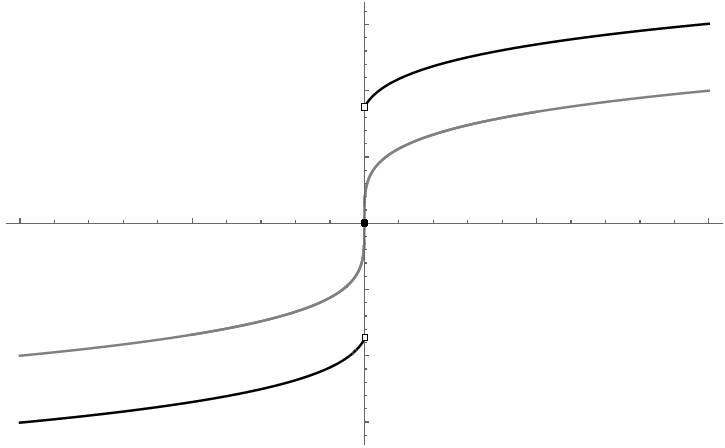
Then and
| (21) |
for , where denotes the maximal lifetime of the smooth solution. Provided does not break down earlier, forms at least a cusp at time (or a potentially stronger singularity, see Fig. 2).
Note that a function with the properties in the Theorem exists for any given . Our theorem does not exclude the possibility of a singularity forming before . However, we offer the following conjecture.
Conjecture 1
If for , then singularity formation can only happen at , i.e. if for some , then the smooth solution can be continued past . In this case we have that the profile of converges to an odd cusp at the singularity.
3 Proofs of main results
Proposition 1
For all , we have the estimates
| (22) | ||||
with a universal constant .
Proof
We estimate
| (23) | ||||
| (24) | ||||
| (25) |
after making the substitution . Now note that for , , hence with
| (26) |
the estimate holds. Note that on account of . Straightforward computations show that for , hence the first line of (22) holds. To continue with the second line of (22), we first note
| (27) |
where is an even function and the integral is absolutely convergent. Similar estimations now show the second line and third line of (22).
3.1 Proof of Theorem 2.1 (Local Existence and Uniqueness)
The proof consists of two parts. We first construct global solutions of of an approximate problem. The following a-priori bounds are crucial:
Proposition 2
Suppose , is odd and
| (28) |
Let solve the equation where the velocity field satisfies
| (29) | |||
| (30) | |||
| (31) |
for all and some . Then there exists a time and a depending only on and such that
| (32) |
holds.
Proof
Along any particle trajectory we compute
| (33) | |||
| (34) | |||
| (35) | |||
| (36) | |||
| (37) | |||
| (38) | |||
| (39) | |||
| (40) |
where we have used . A similar computation shows that
| (41) |
and hence there exists a depending only on such that is bounded by a constant on . To prove a similar bound for , we observe that
| (42) | |||
| (43) | |||
| (44) | |||
| (45) | |||
| (46) | |||
| (47) | |||
| (48) | |||
| (49) |
with some universal . A similar lower bound for exists. We hence get an a-priori bound for . A similar argument for completes (32).
We now define a family of regularized problems. Set
| (50) |
where with being a smooth, nonincreasing function with the properties
| (51) | |||
| (52) |
Now define for odd
| (53) |
which can also be written as
| (54) |
We note the following estimates:
| (55) | ||||
with some universal . This is shown similarly as in Proposition 1, noting that the regularized kernel is bounded by the original kernel . On the other hand, we have estimates of the form
| (56) | ||||
with as .
Proposition 3
For all , the regularized problems
| (57) |
have solutions .
Proof
The first step is to show the local-in-time existence of solutions using the particle trajectory method (see MajdaBertozzi ). The flow map satisfies the following equation:
or equivalently
| (58) |
Here, for a given a flow map , we define
| (59) |
This means, (58) is an equation for with velocity field given by (54) and given by (59). Moreover, a solution of (58) translates into a solution of (57) via relation (59).
We define the operator formally by
| (60) |
with defined by the expression (54) where is given by (59). Then solving (57) is equivalent to solving the fixed point equation
Next we need to introduce a suitable metric space on which is well defined and a contraction. To ease notation, we now fix and henceforth drop the subscript .
Definition 1
Let be the set of all with the following properties:
| (61) | |||
| (62) |
Moreover, is of the form
| (63) |
where means the mapping and
| (64) |
is a complete metric space with metric
Note that for sufficiently small and for any and
is a diffeomorphism of onto . To show that, we first note that by (62). The derivative is given by and is also uniformly bounded away from zero for small . We also see now that is well-defined.
The rest of the proof is standard. First one shows that for sufficiently small that maps into and is a contraction. Note that the -dependent estimates (56) are crucial for the self-mapping and contraction properties. By the contraction mapping theorem there exists a unique solution of (58) on some small time-interval .
The local-in-time solution of the regularized problem (for any fixed ) is easily extended to by standard arguments, noting that the a-priori bound
| (65) |
holds independent of the length of the time interval .
3.2 Proof of Theorem 2.2 (Singularity Formation)
Preliminaries
We need a few preliminary propositions first.
Proposition 4
Let be a smooth function with and define
| (66) |
with . Then
| (67) |
where
| (68) |
Moreover,
-
•
-
•
-
•
as with some .
Proof
We have
| (69) | ||||
| (70) | ||||
| (71) |
after substituting in the integral. Hence the representation (67) holds. From the form of , we directly see that , since the integrand is . To see that we compute
| (72) |
and note that the integral in curly brackets converges to a positive constant as , as can be seen using the dominated convergence theorem. To see , we write
| (73) |
and note .
Lemma 1
Let satisfy all the assumptions of Theorem 2.2. Let be the maximal life-time of the smooth solution . Then for all and all ,
| (74) |
Moreover, there exists a so that for .
Proof
To prove the statement referring to , we first note that for any , there exists a particle trajectory
| (75) |
such that . The assumptions of Theorem 2.2 imply in particular that is always non-negative, so that is non-positive for . Hence the particle trajectory originates from a point and we have, by (16),
since our choice of (see (20)) guarantees the inequality
implying for all .
To argue that the second statement of the Lemma holds, we show first the existence of an and an such that on . The assumption implies for for some small . Smoothness of in time implies that for and some . Because of , we then conclude by integrating with respect to that on . To complete the proof of the second part of the proposition, we choose a such that on and set .
Lemma 2
Let all the assumptions of Theorem 2.2 hold. Define a time by
Suppose also for this proposition that
| (76) |
Then if
| (77) |
As a consequence, there exists a such that for all .
Proof
The supremum defining is because of Lemma 1. The equation (4) and imply for short times
| (78) |
because for small . Observe that for all . Using this, we get for
| (79) | ||||
| (80) |
Moreover the assumption (83) implies, on account of and (76),
from which by taking the limit and using we get
| (81) |
Combining (78), (80) and (81), we get for small
| (82) |
The inequality (82) remains valid as long as . By direct calculation, one finds that for all and hence the inequality holds up to . By taking into account that for small positive and integrating (82) up to we arrive at (77).
Proposition 5
Proof
Define as in Lemma 2 and assume that the conclusion of the Proposition is false, i.e. . Then there exists a sequence with , and by Lemmas 1 and 2, . By passing to a subsequence, we have . As a consequence, we have for some .
Let denote any particle trajectory defined by
| (84) |
where and such that . Observe that
since otherwise by backtracking the trajectory we see that at all times with small and positions , holds, in contradiction to the definition of . Then,
| (85) | |||
| (86) |
where we have used for all to conclude
| (87) |
Hence in summary we get at the relationship
| (88) |
a contradiction.
Proposition 6
Let . There exists a positive constant such that
| (89) |
Proof
We calculate and note that for all . Now observe that by Proposition 4, for small with some and furthermore that for small . Hence there exists a such that
| (90) |
for some . As , and . Using again , we conclude the existence of an so that
| (91) |
for some . The statement of the Proposition now follows since is continuous in and never zero in .
Proof of Theorem 2.2
We now turn to Theorem 2.2. We need to check the following: satisfies
| (92) |
To prove this, we first compute the left hand side using (14) and Proposition 4:
| (93) |
and so is equivalent to
| (94) |
for all . By Proposition 6, (94) is implied by
| (95) |
so is sufficient for (92) to hold, since . By applying Proposition 5, we see that as long as . Note that now necessarily , since in the case the inequality and would imply that has an infinite slope at . This completes the proof of Theorem 2.2.
4 Acknowledgements
The authors would like to thank the anonymous reviewer for a careful reading of this manuscript, many helpful comments, and in particular for pointing out a gap in the first version. We would also like to thank D. Li for very helpful comments on a preprint version of this paper, indicating a related gap. Vu Hoang wishes to thank the National Science Foundation for support under grants NSF DMS-1614797 and NSF DMS-1810687.
References
- (1) K. Choi, T.Y. Hou, A. Kiselev, G. Luo, V. Šverák and Y. Yao, On the Finite-Time Blowup of a One-Dimensional Model for the Three-Dimensional Axisymmetric Euler Equations. Communications on Pure and Applied Mathematics, vol. 70, no. 11, Nov. 2017, pp. 2218–43. Scopus, doi:10.1002/cpa.21697.
- (2) K. Choi, A. Kiselev and Y. Yao, Finite time blow up for a 1d model of 2d Boussinesq system. Comm. Math. Phys., 334(3):1667–1679, 2015.
- (3) P. Constantin, P.D. Lax and A. Majda, A simple one-dimensional model for the three-dimensional vorticity equation, Comm. Pure Appl. Math., 38:715–724, 1985.
- (4) P. Constantin, A. Majda and E. Tabak Formation of strong fronts in the 2-d quasigeostrophic thermal active scalar, Nonlinearity, 7(6):1495–1533, 1994.
- (5) A. Córdoba, D. Córdoba and M.A. Fontelos, Formation of singularities for a transport equation with nonlocal velocity, Ann. of Math.(2), 162(3):1377–1389, 2005.
- (6) Hongjie Dong and Dong Li. On a one-dimensional -patch model with nonlocal drift and fractional dissipation. Trans. Amer. Math. Soc., 366(4):2041–2061, 2014.
- (7) V. Hoang, M. Radosz, Cusp formation for a nonlocal evolution equation, Archive for Rational Mechanics and Analysis, June 2017, Volume 224, Issue 3, pp 1021–1036, https://doi.org/10.1007/s00205-017-1094-3
- (8) V. Hoang, B. Orcan-Ekmeckci, M. Radosz and H. Yang, Blowup with vorticity control for a 2D model of the Boussinesq equations. Journal of Differential Equations, Vol. 264 (12), p.7328–7356 (2018).
- (9) T. Y. Hou and, G. Luo, On the finite-time blowup of a 1D model for the 3D incompressible Euler equations, arXiv:1311.2613.
- (10) T.Y. Hou and G. Luo, Potentially singular solutions of the 3D axisymmetric Euler equations. PNAS, vol. 111 no. 36, 12968–12973, DOI 10.1073/pnas.1405238111.
- (11) T.Y. Hou and C. Li, Dynamic stability of the three-dimensional axisymmetric Navier-Stokes equations with swirl, Commun. Pure Appl. Math, vol. LXI, 661-697 (2008)
- (12) A. Kiselev and V. Šverák. Small scale creation for solutions of the incompressible two dimensional Euler equation. Ann. of Math.(2), 180(3):1205–1220, 2014.
- (13) A. Madja, A. Bertozzi, Vorticity and Incompressible Flow, Cambridge University Press, 2002.
- (14) J. Pedlosky, Geophysical fluid dynamics, Springer Verlag, New York (1979)