Equivalent Hamiltonian approach to quantum cosmology of integrable models

Abstract

We propose an approach to quantum cosmology of integrable models. To analyze the models with two dynamical variables, we introduce equivalent Hamiltonians in reduced phase spaces, which are obtained with the aid of the Faddeev–Jackiw method. Quantum dynamics of the models can be studied by using the equivalent Hamiltonians with various techniques.

I Introduction

In study of quantum cosmology HH ; Hawking ; Halliwell ; Kiefer0 , the probabilistic interpretation of the wave function of the Universe has not been well-defined, because the Wheeler–DeWitt wave equation, which comes from the Hamiltonian constraint, is the second order differential equation in terms of the minisuperspace variables. In other words, one can hardly extract any conserved probability current from the Wheeler–DeWitt wave function of the Universe.

The problem of the probability distribution is closely related to the problem of time in quantum cosmology. If the basic equation is the Schrödinger-type equation that is the first-order differential equation in time, one can obtain the probability density as the absolute square of the wave function.

Many attempts have been made to define a time variable in quantum cosmology: some authors found ‘global time’ Hajicek ; Simeone , and others defined ‘extrinsic time’ CF or ‘conformal time’ Kuzmichev , etc.. Especially, various models defined in two dimensional minisuperspace have been investigated in this context, and one soluble variable in such a model often plays a role of a standard ‘clock’ in the Universe. The other approaches utilize decomposition of the Hamiltonian and the wave function Mostafazadeh or introduce an effective Hamiltonian HA . Even in the former attempt for defining the time, of course, the Hamiltonian defined in each work is different from the original one in a certain sense.

In the present paper, we propose another type of equivalent Hamiltonians for two integrable models. We adopt a heuristic approach to obtain an equivalent Hamiltonian. The general idea of treating a constraint system is explained in the following text in the succeeding section.

The structure of the present paper is as follows. In Sec. II, we specify the first model we treat here, the Liouville scalar model. Although an equivalent Hamiltonian is introduced by a heuristic consideration, the idea of this ‘trick’ is briefly addressed here. Another model, the conformal scalar model is presented in Sec. III. In Sec. IV, we manage to extract quantum nature of the Liouville scalar model by using the equivalent Hamiltonians and the method of cumulants. In Sec. V, we treat the wave function of the conformal scalar model. We examine usefulness of the Gaussian wave packet and the Wigner function in the model. The last section is devoted to conclusion and prospect. In Appendix A, we describe the canonical transform of the Liouville mechanics.

II the Liouville scalar model

II.1 The original system

The cosmological gravitational model of a scalar field with an exponential potential has been studied by many authors until recent times (see, for example, Refs. Russo ; Neupane ; ENO ). We call the model as the Liouville scalar model. We start with the field theoretic action

$$S=\int d^{4}x\sqrt{-g}\left[R-\frac{1}{2}(\nabla\Phi)^{2}-\frac{V}{2}e^{2\alpha\Phi}\right]\,,$$ (1)

where $R$ is the Ricci scalar derived from the metric $g_{\mu\nu}$ ($\mu,\nu=0,1,2,3$), $g$ is the determinant of $g_{\mu\nu}$, and $\Phi$ is a real scalar field. The constant $\alpha$ denotes the scalar self-coupling. We used the abbreviation $(\nabla\Phi)^{2}\equiv g^{\mu\nu}\partial_{\mu}\Phi\partial_{\nu}\Phi$. We also assumed that $V$ is a constant. It is known that the exponential potential of this type can be found in effective field theories of string theory, higher dimensional gravity, and higher derivative gravity (see, for example, Ref. KKST and references there in).

We take an ansatz for the metric tensor as

$$ds^{2}=-N^{2}e^{6b(t)}dt^{2}+e^{2b(t)}d\mathbf{x}^{2}\,,$$ (2)

where $t=x^{0}$, $d\mathbf{x}^{2}\equiv\sum_{\mu=i}^{3}(dx^{i})^{2}$, and $N$ is the lapse function. We also assume that the scalar field $\Phi$ is expressed by the function of $t$. Then, we find

$$S\propto\int dt\,N\left[-6\frac{\dot{b}^{2}}{N^{2}}+\frac{1}{2}\frac{\dot{\Phi}^{2}}{N^{2}}-\frac{V}{2}e^{2\alpha\Phi}e^{6b}\right]\,,$$ (3)

where the dot indicates the derivative with respect to time $t$ and total derivatives have been dropped.

If we choose the following new variables and the defined constants

$$x(t)\equiv\sqrt{12}\left({b}+\frac{\alpha}{3}{\Phi}\right)\,,\quad y(t)\equiv{\Phi}+4{\alpha}{b}\,,$$ (4)

and

$$\lambda\equiv\sqrt{\frac{3}{4}}\,,\quad U\equiv\left(1-\frac{4}{3}{\alpha^{2}}\right)V\,,$$ (5)

the effective Lagrangian is now written by

$$L_{N}=N\left[-\frac{1}{2}\frac{\dot{x}^{2}}{N^{2}}-\frac{U}{2}e^{2\lambda x}+\frac{1}{2}\frac{\dot{y}^{2}}{N^{2}}\right]\,.$$ (6)

The variation in the lapse function leads to $\frac{\partial L_{N}}{\partial N}=0$, that is,

$$-\frac{1}{2}{\dot{x}^{2}}+\frac{U}{2}e^{2\lambda x}+\frac{1}{2}{\dot{y}^{2}}=0\,,$$ (7)

where we redefine $Nt\rightarrow t$, or equivalently, set $N=1$. This is equivalent to the Hamiltonian constraint, which can be regarded as a consequence of reparametrization invariance of $t$. Note that, because of the reparametrization invariance of $t$, the overall normalizations of the Lagrangians and the Hamiltonians which we encounter in this paper are irrelevant for physics of cosmology.

Now, from the Lagrangian

$$L_{1}=-\frac{1}{2}{\dot{x}^{2}}-\frac{U}{2}e^{2\lambda x}+\frac{1}{2}{\dot{y}^{2}}\,,$$ (8)

we can derive the equations of motion as

$$\ddot{x}-\lambda Ue^{2\lambda x}=0\,,\quad\ddot{y}=0\,.$$ (9)

Note that these equations have time-reversal invariance (under $t\rightarrow-t$). Moreover, we obtain corresponding canonical momenta as

$$\pi_{x}=\frac{\partial L_{1}}{\partial\dot{x}}=-\dot{x}\,,\quad\pi_{y}=\frac{\partial L_{1}}{\partial\dot{y}}=\dot{y}\,.$$ (10)

Then, the Hamiltonian of the Liouville scalar model is found to be

$$H=\pi_{x}\dot{x}+\pi_{y}\dot{y}-L_{1}=-\frac{1}{2}{\pi_{x}^{2}}+\frac{U}{2}e^{2\lambda x}+\frac{1}{2}{\pi_{y}^{2}}\,.$$ (11)

One can easily confirm the Hamilton’s equations

$$\dot{x}=\frac{\partial H}{\partial\pi_{x}}=-\pi_{x}\,,\quad\dot{y}=\frac{\partial H}{\partial\pi_{y}}=\pi_{y}\,,\quad\dot{\pi}_{x}=-\frac{\partial H}{\partial x}=-\lambda Ue^{2\lambda x}\,,\quad\dot{\pi}_{y}=-\frac{\partial H}{\partial y}=0\,,$$ (12)

reproduce the classical equation of motion (9).

II.2 An equivalent system

Let us begin with the following set of the first-order differential equations:

$$\dot{x}=\sqrt{U}e^{\lambda x}\cosh\lambda(y-y_{0})\,,\quad\dot{y}=-\sqrt{U}e^{\lambda x}\sinh\lambda(y-y_{0})\,,\quad(U>0)$$ (13)

$$\dot{x}=\sqrt{|U|}e^{\lambda x}\sinh\lambda(y-y_{0})\,,\quad\dot{y}=-\sqrt{|U|}e^{\lambda x}\cosh\lambda(y-y_{0})\,,\quad(U<0)$$ (14)

where $y_{0}$ is a constant.

One can easily verify that, if (13) or (14) holds, the Hamiltonian constraint (7) and the equations of motion (9) are satisfied. The solutions of (13) and (14) are

$$x(t)=\frac{1}{2\lambda}\ln\frac{\pi_{y0}^{2}}{U\sinh^{2}\lambda\pi_{y0}(t-t_{0})}\,,\quad y(t)=\pi_{y0}(t-t_{0})+y_{0}\,,\quad(U>0)$$ (15)

and

$$x(t)=\frac{1}{2\lambda}\ln\frac{\pi_{y0}^{2}}{|U|\cosh^{2}\lambda\pi_{y0}(t-t_{0})}\,,\quad y(t)=\pi_{y0}(t-t_{0})+y_{0}\,,\quad(U<0)$$ (16)

respectively, where $\pi_{y0}$ and $t_{0}$ are integration constants. If we regard $y_{0}$ as another ‘integration constant’, (15) and (16) are general solutions of Eqs. (7) and (9). The degrees of freedom of the solutions are given by the number of integration constants. The solutions of the original equations of motion have $2\times 2=4$ constants. Joining together with one constraint, we have $4-1=3$ constants which are arbitrarily chosen. The first-order equations (13) or (14) yields two integration constants but the choice of $y_{0}$ is arbitrary. Thus, we again obtain $2+1=3$ degrees of freedom. We can conclude that the necessary condition for the similar conversion of the equations of motion is the existence of a ‘cyclic coordinate’ in the original system. In the Liouville scalar model, $y$ is the cyclic coordinate in the minisuperspace, since $\frac{\partial H}{\partial y}=0$.

Note that the Lagrangian can be rewritten as

$$L_{1} = -\frac{1}{2}\left[\dot{x}-\sqrt{U}e^{\lambda x}\cosh\lambda(y-y_{0})\right]^{2}+\frac{1}{2}\left[\dot{y}+\sqrt{U}e^{\lambda x}\sinh\lambda(y-y_{0})\right]^{2}$$ (17)

$$-\frac{d}{dt}\left[\lambda^{-1}\sqrt{U}e^{\lambda x}\cosh\lambda(y-y_{0})\right]\,,\quad(U>0)$$

$$L_{1} = -\frac{1}{2}\left[\dot{x}-\sqrt{|U|}e^{\lambda x}\sinh\lambda(y-y_{0})\right]^{2}+\frac{1}{2}\left[\dot{y}+\sqrt{|U|}e^{\lambda x}\cosh\lambda(y-y_{0})\right]^{2}$$ (18)

$$-\frac{d}{dt}\left[\lambda^{-1}\sqrt{|U|}e^{\lambda x}\sinh\lambda(y-y_{0})\right]\,.\quad(U<0)$$

Now, we introduce a new equivalent system. We find that Eqs. (13) and (14) can also be derived from the following first-order Lagrangian:

$$\bar{L} = (y-y_{0})\dot{x}-\lambda^{-1}\sqrt{U}e^{\lambda x}\sinh\lambda(y-y_{0})\,,\quad(U>0)$$ (19)

$$\bar{L} = (y-y_{0})\dot{x}-\lambda^{-1}\sqrt{|U|}e^{\lambda x}\cosh\lambda(y-y_{0})\,.\quad(U<0)$$ (20)

According to the prescription of Faddeev and Jackiw FJ ; Jackiw , the Hamiltonian of this equivalent system is

$$\bar{H} = \lambda^{-1}\sqrt{U}e^{\lambda x}\sinh\lambda p\,,\quad(U>0)$$ (21)

$$\bar{H} = \lambda^{-1}\sqrt{|U|}e^{\lambda x}\cosh\lambda p\,,\quad(U<0)$$ (22)

where $p$ is the conjugate momentum of $x$.

The Hamilton’s equations are found to be

$$\dot{x}=\frac{\partial\bar{H}}{\partial p}=\sqrt{U}e^{\lambda x}\cosh\lambda p\,,\quad\dot{p}=-\frac{\partial\bar{H}}{\partial x}=-\sqrt{U}e^{\lambda x}\sinh\lambda p\,,\quad(U>0)$$ (23)

$$\dot{x}=\frac{\partial\bar{H}}{\partial p}=\sqrt{|U|}e^{\lambda x}\sinh\lambda p\,,\quad\dot{p}=-\frac{\partial\bar{H}}{\partial x}=-\sqrt{|U|}e^{\lambda x}\cosh\lambda p\,,\quad(U<0)$$ (24)

which are surely equivalent to (13) and (14), respectively, provided that we regard $p\approx y-y_{0}$ (where “$\approx$” means “is identified with”).

The idea of our prescription originates from the canonical transformation of the Liouville Hamiltonian Ghandour . If the Liouville Hamiltonian reduces to the form of $\frac{1}{2}\Pi^{2}$ (see Appendix A), we can choose the Hamiltonian constraint as $\Pi\pm\pi_{y}=0$, instead of $-\Pi^{2}+\pi_{y}^{2}=0$. Our further step is to propose that the classical constraint is expressed in the first-order Lagrangian à la Faddeev and Jackiw FJ ; Jackiw and then we can obtain the equivalent Hamiltonian $\bar{H}$ of a reduced set of canonical variables, $x$ and $p$. Thus, $y-y_{0}\approx p$ plays a role of a universal ‘clock’.

In the next section, we show another model, the conformal scalar model and its equivalent Hamiltonian. The study of quantum dynamics of two models will be described in Sec. IV and Sec. V.

III the conformal scalar model

III.1 The original system

The simplest model for a spatially homogeneous and isotropic Universe is described by the action HH ; Hawking ; Kiefer2

$$S=\int d^{4}x\sqrt{-g}\left[R-\frac{1}{2}(\nabla\phi)^{2}-\frac{1}{12}R\phi^{2}\right]\,,$$ (25)

where $\phi$ is a real scalar field conformally coupled to the scalar curvature. We consider this system in the minisuperspace as the second example of the integrable model in this paper and call it the conformal scalar model.

We take an ansatz for the metric tensor as

$$ds^{2}=a^{2}(t)\left[-N^{2}dt^{2}+\frac{d\rho^{2}}{1-k\rho^{2}}+\rho^{2}(d\theta^{2}+\sin^{2}\theta d\psi^{2})\right]\,,$$ (26)

where $k(=\pm 1)$ indicates the sign of the spatial curvature. We also assume that the conformally invariant scalar field $\phi$ is expressed by the function of $t$. Then, we find

$$S\propto 12\int dt\,N\left[-\frac{1}{2}\frac{\dot{a}^{2}}{N^{2}}+\frac{k}{2}a^{2}+\frac{1}{2}\frac{\dot{\chi}^{2}}{N^{2}}-\frac{k}{2}\chi^{2}\right]\,,$$ (27)

where $\chi=a\phi/\sqrt{12}$ and total derivatives have been dropped. By using new variables

$$a(t)=r(t)\cosh\varphi(t)\,,\quad\chi(t)=r(t)\sinh\varphi(t)\,,$$ (28)

we find a simple form of the Lagrangian

$$L_{1}=-\frac{1}{2}\dot{r}^{2}+\frac{k}{2}r^{2}+\frac{1}{2}r^{2}\dot{\varphi}^{2}\,,$$ (29)

and the constraint

$$-\frac{1}{2}\dot{r}^{2}-\frac{k}{2}r^{2}+\frac{1}{2}r^{2}\dot{\varphi}^{2}=0\,.$$ (30)

Note that the variable $\varphi$ is a ‘cyclic coordinate’ in the two dimensional minisuperspace.

The equations of motion derived from the Lagrangian (29) are

$$\ddot{r}+r\dot{\varphi}^{2}+kr=0\,,\quad\ddot{\varphi}+2\frac{\dot{r}}{r}\dot{\varphi}=0\,.$$ (31)

Note that these equations have time-reversal invariance.

III.2 An equivalent system and canonical transformations

Now, we find that the set of equations

$$\dot{r}=r\sinh 2(\varphi-\varphi_{0})\,,\quad\dot{\varphi}=-\cosh 2(\varphi-\varphi_{0})\,,\quad\mbox{for }k=1\,,$$ (32)

$$\dot{r}=r\cosh 2(\varphi-\varphi_{0})\,,\quad\dot{\varphi}=-\sinh 2(\varphi-\varphi_{0})\,,\quad\mbox{for }k=-1\,,$$ (33)

reproduces the equations of motion (31) and the constraint (30). Here, $\varphi_{0}$ is a constant. Note that the original Lagrangian can be written as

$$L_{1} = -\frac{1}{2}\left[\dot{r}-r\sinh 2(\varphi-\varphi_{0})\right]^{2}+\frac{1}{2}r^{2}\left[\dot{\varphi}+\cosh 2(\varphi-\varphi_{0})\right]^{2}$$ (34)

$$-\frac{d}{dt}\left[\frac{r^{2}}{2}\sinh 2(\varphi-\varphi_{0})\right]\,,\quad\mbox{for }k=1\,,$$

$$L_{1} = -\frac{1}{2}\left[\dot{r}-r\cosh 2(\varphi-\varphi_{0})\right]^{2}+\frac{1}{2}r^{2}\left[\dot{\varphi}+\sinh 2(\varphi-\varphi_{0})\right]^{2}$$ (35)

$$-\frac{d}{dt}\left[\frac{r^{2}}{2}\cosh 2(\varphi-\varphi_{0})\right]\,,\quad\mbox{for }k=-1\,.$$

The Lagrangians which lead to the first-order equations (32) and (33) are

$$\bar{L} = (\varphi-\varphi_{0})r\dot{r}-\frac{r^{2}}{2}\cosh 2(\varphi-\varphi_{0})=(\varphi-\varphi_{0})\dot{q}-q\cosh 2(\varphi-\varphi_{0})\,,~{}~{}\mbox{for }k=1\,,$$ (36)

$$\bar{L} = (\varphi-\varphi_{0})r\dot{r}-\frac{r^{2}}{2}\sinh 2(\varphi-\varphi_{0})=(\varphi-\varphi_{0})\dot{q}-q\sinh 2(\varphi-\varphi_{0})\,,~{}~{}\mbox{for }k=-1\,,$$ (37)

respectively, where we set $q\equiv r^{2}/2$. Now, we can obtain the classical Hamiltonians with the aid of the Faddeev–Jackiw method as in the previous section:

$$\bar{H} = q\cosh 2p\,,\quad\mbox{for }k=1\,,$$ (38)

$$\bar{H} = q\sinh 2p\,,\quad\mbox{for }k=-1\,.$$ (39)

In this model, this is not the final form of physical interest. One can find the Poisson’s bracket $\{Q,P\}=1$, where

$$Q\equiv\sqrt{2q}\cosh p\,,\quad P\equiv\sqrt{2q}\sinh p\,.$$ (40)

Using the new canonical set of variables, the equivalent Hamiltonians read

$$\bar{H} = \frac{1}{2}\left(P^{2}+Q^{2}\right)\,,\quad\mbox{for }k=1\,,$$ (41)

$$\bar{H} = QP\,,\quad\mbox{for }k=-1\,.$$ (42)

To check the validity, we derive the Hamilton’s equations

$$\dot{Q}=\frac{\partial\bar{H}}{\partial P}=P\,,\quad\dot{P}=-\frac{\partial\bar{H}}{\partial Q}=-Q\,,\quad\mbox{for }k=1\,,$$ (43)

$$\dot{Q}=\frac{\partial\bar{H}}{\partial P}=Q\,,\quad\dot{P}=-\frac{\partial\bar{H}}{\partial Q}=-P\,,\quad\mbox{for }k=-1\,.$$ (44)

Note that $p$ was identified with $\varphi-\varphi_{0}$ by the Faddeev–Jackiw method. Hereafter, we again denote the identification by using the symbol “$\approx$” for conciseness. Then, we find

$$Q\approx r\cosh(\varphi-\varphi_{0})=r(\cosh\varphi\cosh\varphi_{0}-\sinh\varphi\sinh\varphi_{0})=a\cosh\varphi_{0}-\chi\sinh\varphi_{0}\,,$$ (45)

$$P\approx r\sinh(\varphi-\varphi_{0})=r(\sinh\varphi\cosh\varphi_{0}-\cosh\varphi\sinh\varphi_{0})=\chi\cosh\varphi_{0}-a\sinh\varphi_{0}\,,$$ (46)

or

$$a\approx Q\cosh\varphi_{0}+P\sinh\varphi_{0}\,,\quad\chi\approx P\cosh\varphi_{0}+Q\sinh\varphi_{0}\,.$$ (47)

After straightforward calculations, one can find that the Hamilton’s equations are equivalent to the first-order equations (32) and (33), as far as we regard $p\approx\varphi-\varphi_{0}$.

The classical solutions of the systems are found to be

$$Q(t)=Q_{0}\cos t+P_{0}\sin t\,,\quad P(t)=P_{0}\cos t-Q_{0}\sin t\,,\quad\mbox{for }k=1\,,$$ (48)

$$Q(t)=Q_{0}\,e^{t}\,,\quad P(t)=P_{0}\,e^{-t}\,,\quad\mbox{for }k=-1\,,$$ (49)

where $Q_{0}$ and $P_{0}$ are constants.

It is remarkable that the conformal scalar model with $k=1$ reduces to a system of a harmonic oscillator while the model with $k=-1$ reduces to the well-known $xp$ model BK99a ; BK99b ; Conne ; Sierra ; ST ; BBM , whose spectrum is considered to be related to the zeros of the Riemann zeta function. Incidentally, it is also known that the similar Hamiltonian has been studied in the model of loop quantum cosmology Bojowald1 ; Bojowald2 .

For the conformal scalar model with $k=-1$, a remarkable canonical transformation remains to be done. The new canonical pair is

$$Q^{\prime}\equiv\frac{Q-P}{\sqrt{2}}\,,\quad P^{\prime}\equiv\frac{P+Q}{\sqrt{2}}\,.$$ (50)

Then, the Hamiltonian is rewritten as

$$\bar{H}=\frac{1}{2}({P^{\prime}}^{2}-{Q^{\prime}}^{2})\,.$$ (51)

This is just a so-called inverted harmonic oscillator. The classical solution of the system can be written as

$$Q^{\prime}(t)=Q^{\prime}_{0}\cosh t+P^{\prime}_{0}\sinh t\,,\quad P^{\prime}(t)=P^{\prime}_{0}\cosh t+Q^{\prime}_{0}\sinh t\,,$$ (52)

where $Q^{\prime}_{0}$ and $P^{\prime}_{0}$ are constants. Note that the correspondence to the original variables is

$$Q^{\prime}\approx\frac{1}{\sqrt{2}}(a-\chi)e^{\varphi_{0}}\,,\quad P^{\prime}\approx\frac{1}{\sqrt{2}}(a+\chi)e^{-\varphi_{0}}\,.$$ (53)

In the next two sections, we will try to investigate the quantum nature of our models.

IV towards quantum dynamics of the Liouville scalar model

If we introduce the wave function of the Universe $\Psi(t,q)$, the Schrödinger equation can be written as

$$i\hbar\frac{\partial\Psi}{\partial t}=\hat{H}\Psi\,,$$ (54)

where $\hbar$ is the Planck’s constant. Here $\hat{H}$ is the ‘quantum Hamiltonian’, usually connected to the classical Hamiltonian $H(q,p)\rightarrow\hat{H}(\hat{q},\hat{p})$, up to the operator ordering.

As a wave equation obtained by replacing $\hat{p}$ with $\frac{\hbar}{i}\frac{\partial}{\partial q}$, the Schrödinger equation for the Liouville scalar model described in Sec. II is hard to solve, because there appear infinite derivatives. We postpone the study on the wave function itself for the future work, here we consider the quantum effects on the classical solutions in the Liouville scalar model. The conformal scalar model will be studied in the next section.

It is well-known that the Ehrenfest’s theorem tells

$$\frac{d\langle\hat{A}\rangle}{dt}=\frac{1}{i\hbar}\langle[\hat{A},\hat{H}]\rangle\,,$$ (55)

where $\langle\hat{A}\rangle$ is the expectation value of the operator $\hat{A}$. The approximation of the equation in the order $\hbar^{0}$ gives the classical equations of motion. To evaluate the quantum corrections, we should treat the fluctuation operator $\delta\hat{A}=\hat{A}-\langle\hat{A}\rangle$ appropriately.

Recently, Shigeta et al.SMH ; Shigeta defined an expression for the expectation value by means of cumulants among the canonical pair of the variables $q$ and $p$. That is defined as

$$\langle A_{S}(\hat{q},\hat{p})\rangle_{M}\equiv\exp\left(\sum_{m=2}^{M}\sum_{0\leq\ell\leq m}\frac{\kappa_{\ell,m-\ell}}{\ell!(m-\ell)!}\frac{\partial_{m}}{\partial q^{\ell}\partial p^{m-\ell}}\right)A(q,p)\,,$$ (56)

where we introduced the cumulants $\kappa_{i,j}\equiv\langle((\delta\hat{q})^{i}(\delta\hat{p})^{j})_{S}\rangle$ $(i,j=0,1,2,\ldots)$ and the subscript $S$ indicates a symmetric sum of the operators defined as $\langle((\delta\hat{q})^{i}(\delta\hat{p})^{j})_{S}\rangle\equiv\frac{1}{2}\langle((\delta\hat{q})^{i}(\delta\hat{p})^{j}+(\delta\hat{p})^{j}(\delta\hat{q})^{i})\rangle$. This definition can be expressed as $\frac{1}{2}\{(\delta\hat{q})^{i},(\delta\hat{p})^{j}\}$, where $\{~{},~{}\}$ denotes the anticommutator.

Here, we takes the approximation by taking $M=2$ and we set the approximated Hamiltonian as

$$\tilde{H}(q,p;\kappa_{2,0},\kappa_{1,1},\kappa_{0,2})\equiv\langle\hat{H}(\hat{q},\hat{p})\rangle_{2}\,.$$ (57)

Then, the following simultaneous equations are derived from the Ehrenfest’s theorem:SMH ; Shigeta

$$\dot{q} = \tilde{H}^{(0,1)}\,,$$ (58)

$$\dot{p} = -\tilde{H}^{(1,0)}\,,$$ (59)

$$\dot{\kappa}_{2,0} = 2\kappa_{2,0}\tilde{H}^{(1,1)}+2\kappa_{1,1}\tilde{H}^{(0,2)}\,,$$ (60)

$$\dot{\kappa}_{1,1} = -\kappa_{2,0}\tilde{H}^{(2,0)}+\kappa_{0,2}\tilde{H}^{(0,2)}\,,$$ (61)

$$\dot{\kappa}_{0,2} = -2\kappa_{1,1}\tilde{H}^{(2,0)}-2\kappa_{0,2}\tilde{H}^{(1,1)}\,,$$ (62)

where $\tilde{H}^{(2,0)}\equiv\frac{\partial^{2}\tilde{H}}{\partial q^{2}}$, $\tilde{H}^{(1,1)}\equiv\frac{\partial^{2}\tilde{H}}{\partial q\partial p}$, and $\tilde{H}^{(0,2)}\equiv\frac{\partial^{2}\tilde{H}}{\partial p^{2}}$.

Accordingly, the approximated Hamiltonian for the Liouville scalar model is calculated as

$$\tilde{H}(x,p;\kappa_{2,0},\kappa_{1,1},\kappa_{0,2}) = \frac{\sqrt{U}}{\lambda}\exp\left[\lambda x+\frac{\lambda^{2}(\kappa_{2,0}+\kappa_{0,2})}{2}\right]\sinh(\lambda p+\lambda^{2}\kappa_{1,1})\,,(U>0)$$ (63)

$$\tilde{H}(x,p;\kappa_{2,0},\kappa_{1,1},\kappa_{0,2}) = \frac{\sqrt{|U|}}{\lambda}\exp\left[\lambda x+\frac{\lambda^{2}(\kappa_{2,0}+\kappa_{0,2})}{2}\right]\cosh(\lambda p+\lambda^{2}\kappa_{1,1})\,,(U<0)$$ (64)

where the canonical pair is replaced by $(q,p)\rightarrow(x,p)$.

Now, we can numerically solve the simultaneous equations (58-62) (with $q\rightarrow x$). Since we know that $p\approx y-y_{0}$ evolves linearly in time in the classical system, we illustrate evolutions of variables as functions of $p$.

(a)                                                                  (b)

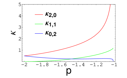
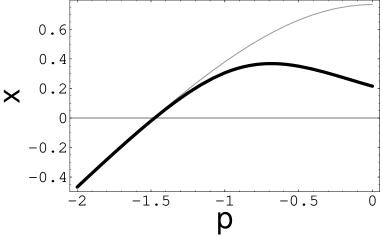
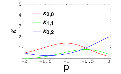
Figure 1: (a) The quantum corrected solution (black curve) for (58-62) and the classical solution (gray curve) under the same initial conditions are plotted in the Liouville scalar model with $U>0$. For the choice of initial values and constants, see the text. (b) The values of the cumulants are plotted against $p$ in the Liouville scalar model with $U>0$. For the choice of initial values and constants, see the text.

Fig. 1 shows the classical solutions and quantum corrections in the Liouville scalar model with $U>0$. We set $\hbar=1$, $\lambda=\sqrt{3}/2$, and $U=3/4$. Initial conditions are given at $p=p_{0}=-2$. We choose $x(p_{0})=-0.96163$, $\kappa_{2,0}(p_{0})=\kappa_{0,2}(p_{0})=1/2$, and $\kappa_{1,1}(p_{0})=0$.

Note that $\kappa_{2,0}\kappa_{0,2}=1/4$ is the minimal value which comes from the uncertainty principle (i.e., we assume a coherent state initially). Note also that $\kappa_{2,0}\kappa_{0,2}-\kappa_{1,1}^{2}$ is a constant SMH ; Shigeta .

In Fig. 1 (a), the quantum corrected solution (black curve) for (58-62) and the classical solution (gray curve) under the same initial condition are plotted. Quantum corrections enhances the value of $x$. In Fig. 1 (b), the value of the cumulants are plotted. Around $p\fallingdotseq-1$, the value of $\kappa_{0,2}$ tends to take a minus value and $\kappa_{2,0}$ grows unlimitedly. This indicates that the point is the limit of the present approximation scheme and we should incorporate higher-order cumulants to obtain precise quantum effects.

(a)                                                                  (b)

Figure 2: (a) The quantum corrected solution (black curve) for (58-62) and the classical solution (gray curve) under the same initial conditions are plotted in the Liouville scalar model with $U<0$. For the choice of initial values and constants, see the text. (b) The value of the cumulants are plotted against $p$ in the Liouville scalar model with $U<0$. For the choice of initial values and constants, see the text.

Fig. 2 shows the classical solutions and quantum corrections in the Liouville scalar model with $U<0$. We set $\hbar=1$, $\lambda=\sqrt{3}/2$, and $U=-1/2$. Initial conditions are given at $p=p_{0}=-2$. We choose $x(p_{0})=-0.467658$, $\kappa_{2,0}(p_{0})=\kappa_{0,2}(p_{0})=1/2$, and $\kappa_{1,1}(p_{0})=0$.

In Fig. 2 (a), the quantum corrected solution (black curve) for (58-62) and the classical solution (gray curve) under the same initial conditions are plotted in the model with $U<0$. Quantum corrections reduces the value of $x$. In Fig. 2 (b), the value of the cumulants are plotted. The evolution of the cumulants in the model with $U<0$ are more moderate than the model with $U>0$.

In both cases, we should consider various cases of squeezed states, i.e., $\kappa_{2,0}\gg\kappa_{0,2}\mbox{ or }\kappa_{2,0}\ll\kappa_{0,2}$, and study the evolution of decoherence in the higher-order approximation, in order to conclude the precise behavior of the quantum Liouville cosmology.

Here, we would like to comment on the realization of the original Hamiltonian constraint (7) in the current equivalent system. From Eqs. (58-64), we find that $\dot{x}^{2}-\dot{y}^{2}=U\exp[2\lambda x+\lambda^{2}(\kappa_{2,0}+\kappa_{0,2})]$. Thus, the constraint is satisfied semiclassically in the sense of the Ehrenfest’s theorem, but the quantum fluctuations (cumulants) may cause deviations. Further study on the constraint in the system is very important and we wish to report on the study in the future.

Before closing this section, we place a comment on a further canonical transformation. Incidentally, if we perform canonical transformation

$$X\equiv\frac{x-p}{\sqrt{2}}\,,\quad P\equiv\frac{x+p}{\sqrt{2}}\,,$$ (65)

on the equivalent Hamiltonians (21) and (22), we obtain

$$\bar{H} = (2\lambda)^{-1}\sqrt{U}[e^{\sqrt{2}\lambda P}-e^{\sqrt{2}\lambda X}]\,,\quad(U>0)$$ (66)

$$\bar{H} = (2\lambda)^{-1}\sqrt{|U|}[e^{\sqrt{2}\lambda P}+e^{\sqrt{2}\lambda X}]\,,\quad(U<0)$$ (67)

as the Hamiltonians. Similar types of Hamiltonians have been studied in an area of mathematical physics recently, see for example FT ; GHM ; LST ; CMS ; MZ ; GM . We should further study the Liouville scalar model of quantum universe in the future work, considering the help of various possible ways to investigate it.

V quantum dynamics and wave function of the conformal scalar model

V.1 Cumulant quantum dynamics of the conformal scalar model

Incidentally, for the conformal scalar model, we find the quantum Hamiltonian formulated in the previous section as

$$\tilde{H}(Q,P;\kappa_{2,0},\kappa_{1,1},\kappa_{0,2})=\frac{1}{2}\left(P^{2}+\kappa_{0,2}+Q^{2}+\kappa_{2,0}\right)\,,\quad(k=1)$$ (68)

$$\tilde{H}(Q,P;\kappa_{2,0},\kappa_{1,1},\kappa_{0,2})=\left(QP\right)_{S}+\kappa_{1,1}\,.\quad(k=-1)$$ (69)

Note that these are also exact quantum Hamiltonians up to the all order $M=\infty$. It can be seen from the quantum Hamiltonians and the simultaneous equations (58-62) in which the dynamics of the expectation values of $Q$ and $P$ and the dynamics of the cumulants are completely decoupled in the conformal scalar model in the both cases $k=1$ and $k=-1$. Thus, the solutions for $Q$ and $P$ coincide with the classical solutions (48) and (49) for $k=1$ and $k=-1$, respectively. The solutions for the cumulants are $\kappa_{2,0}=A-B\cos 2(t-t_{1})$, $\kappa_{0,2}=A+B\cos 2(t-t_{1})$, and $\kappa_{1,1}=B\sin 2(t-t_{1})$ for $k=1$, while $\kappa_{2,0}=A\exp[2(t-t_{1})]$, $\kappa_{0,2}=A\exp[-2(t-t_{1})]$, and $\kappa_{1,1}=B$ for $k=-1$. We used $A$, $B$, and $t_{1}$ as integration constants here. Therefore, we find that the magnitude of coherence of the initial state becomes oscillatory in the conformal scalar model with $k=1$ while the decoherence develops in the conformal scalar model with $k=-1$.

V.2 The wave function and the Wigner function of the conformal scalar model with $k=1$

Especially, since an arbitrary state of the conformal scalar model with $k=1$ can be expressed by the states of a harmonic oscillator, a wave packet corresponding to a semiclassical evolution can be described by superposition of eigenstates. Particularly, a coherent state is interesting as an initial state.

We can analyze the conformal scalar model with $k=1$, which is the simplest toy model of quantum cosmology, by using the known results on harmonic oscillators. According to a typical wave packet exhibited in Ref. RB , a typical wave function in the model with $k=1$ can be written as

$$\Psi(Q,t) = \frac{1}{\sqrt{\pi^{1/2}A(t)}}\exp\left[\frac{i\{(Q^{2}+Q_{0}^{2})\cos t-2Q_{0}Q\}}{2\hbar\sin t}\right]$$ (70)

$$\times\exp\left[-\frac{i\beta}{2\hbar\sin t}\frac{(Q-Q_{0}\cos t-P_{0}\sin t)^{2}}{A(t)}\right]\,,$$

where

$$A(t)\equiv\beta\cos t+i\frac{\hbar}{\beta}\sin t\,,$$ (71)

and $Q_{0}$, $P_{0}$, and $\beta$ are constants. The probability density is given by

$$|\Psi(Q,t)|^{2}=\frac{1}{\sqrt{\pi}|A(t)|}\exp\left[-\frac{(Q-Q_{0}\cos t-P_{0}\sin t)^{2}}{|A(t)|^{2}}\right]\,.$$ (72)

The initial wave packet gives $\langle Q\rangle=Q_{0}$ for $t=0$. Note that the second order cumulant $\kappa_{2,0}$ is given by $|A(t)|^{2}=\frac{\hbar}{2}\left(\frac{\beta^{2}}{\hbar}\cos^{2}t+\frac{\hbar}{\beta^{2}}\sin^{2}t\right)$. The initial condition on the coherence is given by the constant $\beta$ and $\beta=\sqrt{\hbar}$ gives a coherent state and then $|A(t)|^{2}=\hbar/2$.

Generally speaking, the Wigner function Wigner ; Case ; WF is defined, in terms of a wave function $\phi(q)$, by

$$W(q,p)\equiv\frac{1}{2\pi\hbar}\int_{-\infty}^{\infty}du\,\phi^{*}\left(q-\frac{u}{2}\right)\phi\left(q+\frac{u}{2}\right)e^{-i\frac{p}{\hbar}u}\,.$$ (73)

The Wigner function has beautiful properties, such as

$$\int_{-\infty}^{\infty}dp\,W(q,p)=\left|\phi\left(q\right)\right|^{2}\,,\quad\int_{-\infty}^{\infty}dq\,W(q,p)=|\tilde{\phi}\left(p\right)|^{2}\,,$$ (74)

where $\tilde{\phi}(p)$ is the Fourier transform of $\phi(q)$. Note that the Wigner function itself is not positive definite in general.

For the Gaussian wave packet of a harmonic oscillator, the simple result of the Wigner function has already been known Case . In the present model, the Wigner function is given by

$$W(Q,P,t)=\frac{1}{\pi\hbar}\exp\left[-\frac{1}{\beta^{2}}(Q\cos t-P\sin t-Q_{0})^{2}-\frac{\beta^{2}}{\hbar^{2}}(P\cos t+Q\sin t-P_{0})^{2}\right]\,.$$ (75)

It is remarkable that the Wigner function is positive in this case.

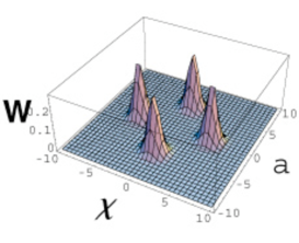
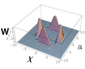
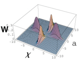
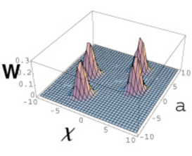
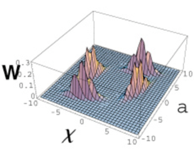
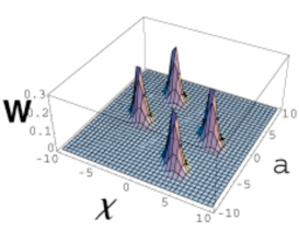
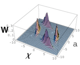
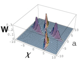
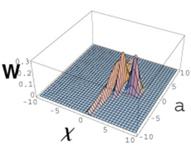
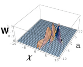
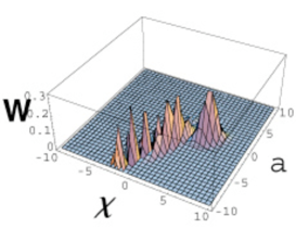
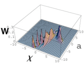
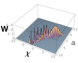
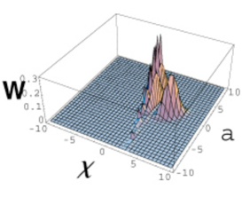
Remembering the relation between $(Q,P)$ and $(a,\chi)$ (47) in Sec. III, we can plot the Wigner function as a two-parameter function of $a$ and $\chi$. We set $\hbar=1$, and $a(0)=0$ and $\chi(0)=5$ in the following figures. Fig. 3 shows the Wigner functions of (a) a coherent state, $\beta=1$, (b) a squeezed state, $\beta=2$ and (c) a squeezed state, $\beta=1/2$, for $\varphi_{0}=0$. Fig. 4 shows the Wigner functions of the same states for $\varphi_{0}=0.3$. Fig. 5 shows the Wigner functions of the same states for $\varphi_{0}=-0.3$. In each figure, the Wigner function at times $t=0$, $t=\pi/2$, $t=\pi$, and $t=3\pi/2$ are shown at once.

(a)                                             (b)                                             (c)

Figure 3: Plots of the Wigner functions of (a) a coherent state, $\beta=1$, (b) a squeezed state, $\beta=2$ and (c) a squeezed state, $\beta=1/2$, for $\varphi_{0}=0$ in the conformal scalar model with $k=1$. In each figure, the Wigner function at times $t=0$, $t=\pi/2$, $t=\pi$, and $t=3\pi/2$ are shown at once.

(a)                                             (b)                                             (c)

Figure 4: Plots of the Wigner functions of (a) a coherent state, $\beta=1$, (b) a squeezed state, $\beta=2$ and (c) a squeezed state, $\beta=1/2$, for $\varphi_{0}=0.3$ in the conformal scalar model with $k=1$. In each figure, the Wigner function at times $t=0$, $t=\pi/2$, $t=\pi$, and $t=3\pi/2$ are shown at once.

(a)                                             (b)                                             (c)

Figure 5: Plots of the Wigner functions of (a) a coherent state, $\beta=1$, (b) a squeezed state, $\beta=2$ and (c) a squeezed state, $\beta=1/2$, for $\varphi_{0}=-0.3$ in the conformal scalar model with $k=1$. In each figure, the Wigner function at times $t=0$, $t=\pi/2$, $t=\pi$, and $t=3\pi/2$ are shown at once.

As already seen from the analysis with cumulants, the behavior of the Gaussian wave packet seems very simple and its behavior seems similar to, or consistent with, the result from the analysis of the wave packet of Wheeler–DeWitt equation in the conformal scalar model Kiefer0 ; Kiefer2 .

V.3 The wave function and the Wigner function of the conformal scalar model with $k=-1$

The equivalent Hamiltonian of the conformal scalar model with $k=-1$ can be expressed by that of an inverted harmonic oscillator, as (51) in Sec. III. A typical Gaussian wave function in our model (with $k=-1$) can be written as

$$\Psi(Q^{\prime},t) = \frac{1}{\sqrt{\pi^{1/2}A(t)}}\exp\left[\frac{i\{({Q^{\prime}}^{2}+{Q^{\prime}_{0}}^{2})\cosh t-2Q^{\prime}_{0}Q^{\prime}\}}{2\hbar\sinh t}\right]$$ (76)

$$\times\exp\left[-\frac{i\beta}{2\hbar\sinh t}\frac{(Q^{\prime}-Q^{\prime}_{0}\cosh t-P^{\prime}_{0}\sinh t)^{2}}{A(t)}\right]\,,$$

where

$$A(t)\equiv\beta\cosh t+i\frac{\hbar}{\beta}\sinh t\,,$$ (77)

and $Q^{\prime}_{0}$, $P^{\prime}_{0}$, and $\beta$ are constants. The probability density is given by

$$|\Psi(Q^{\prime},t)|^{2}=\frac{1}{\sqrt{\pi}|A(t)|}\exp\left[-\frac{(Q^{\prime}-Q^{\prime}_{0}\cosh t-P^{\prime}_{0}\sinh t)^{2}}{|A(t)|^{2}}\right]\,.$$ (78)

The initial wave packet gives $\langle Q^{\prime}\rangle=Q^{\prime}_{0}$ at $t=0$. Note that the second order cumulant $\kappa_{2,0}$ is given by $|A(t)|^{2}=\frac{\hbar}{2}\left(\frac{\beta^{2}}{\hbar}\cosh^{2}t+\frac{\hbar}{\beta^{2}}\sinh^{2}t\right)$. The initial condition on the coherence is given by the constant $\beta$ and $\beta=\sqrt{\hbar}$ gives a coherent state. In this case, $|A(t)|^{2}=(\hbar/2)\cosh 2t$.

The Wigner function of the Gaussian wave packet in the model with $k=-1$ is given by

$$W(Q^{\prime},P^{\prime},t)$$

$$=\frac{1}{\pi\hbar}\exp\left[-\frac{1}{\beta^{2}}(Q^{\prime}\cosh t-P^{\prime}\sinh t-Q^{\prime}_{0})^{2}-\frac{\beta^{2}}{\hbar^{2}}(P^{\prime}\cosh t-Q^{\prime}\sinh t-P^{\prime}_{0})^{2}\right]\,.$$ (79)

Note that the Wigner function is also positive in this case.

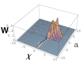
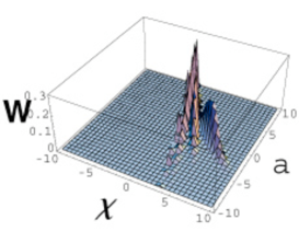
Remembering the relation $(Q^{\prime},P^{\prime})$ and $(a,\chi)$ (53) in Sec. III, we can plot the Wigner function as a two-parameter function of $a$ and $\chi$. We set $\hbar=1$, and $a(0)=0$ and $\chi(0)=5$ in the figures. Fig. 6 shows the Wigner functions of (a) a coherent state, $\beta=1$, (b) a squeezed state, $\beta=2$ and (c) a squeezed state, $\beta=1/2$, for $\varphi_{0}=0$. Fig. 7 shows the Wigner functions of the same states for $\varphi_{0}=0.3$. Fig. 8 shows the Wigner functions of the same states for $\varphi_{0}=-0.3$. In each figure, the Wigner function at times $t=0$, $t=\pi/4$, $t=\pi/2$, and $t=3\pi/4$ are shown at once.

(a)                                             (b)                                             (c)

Figure 6: Plots of the Wigner functions of (a) a coherent state, $\beta=1$, (b) a squeezed state, $\beta=2$ and (c) a squeezed state, $\beta=1/2$, for $\varphi_{0}=0$ in the conformal scalar model with $k=-1$. In each figure, the Wigner function at times $t=0$, $t=\pi/4$, $t=\pi/2$, and $t=3\pi/4$ are shown at once.

(a)                                             (b)                                             (c)

Figure 7: Plots of the Wigner functions of (a) a coherent state, $\beta=1$, (b) a squeezed state, $\beta=2$ and (c) a squeezed state, $\beta=1/2$, for $\varphi_{0}=0.3$ in the conformal scalar model with $k=-1$. In each figure, the Wigner function at times $t=0$, $t=\pi/4$, $t=\pi/2$, and $t=3\pi/4$ are shown at once.

(a)                                             (b)                                             (c)

Figure 8: Plots of the Wigner functions of (a) a coherent state, $\beta=1$, (b) a squeezed state, $\beta=2$ and (c) a squeezed state, $\beta=1/2$, for $\varphi_{0}=-0.3$ in the conformal scalar model with $k=-1$. In each figure, the Wigner function at times $t=0$, $t=\pi/4$, $t=\pi/2$, and $t=3\pi/4$ are shown at once.

The Wigner functions directly demonstrate the decoherence of the initial wave packets in the model with $k=-1$.

VI Conclusion

We have provided equivalent Hamiltonians for two integrable cosmological models, in order to have Schrödinger-type equations. In the present paper, we have investigated semiclassical behavior of the models using quantum dynamics incorporating cumulants. In the Liouville scalar model with $U>0$, the value of $\kappa_{0,2}$ tends to take a minus value and $\kappa_{2,0}$ diverges around $p\fallingdotseq-1$. Therefore, we have to incorporate higher order cumulants to obtain precise quantum effect. On the other hand, the evolution of the cumulants in the model with $U<0$ are more moderate than the model with $U>0$. In the conformal scalar model, the wave function has been solved and we found that the Wigner function indicates the time-evolution of the Gaussian wave packet in quantum cosmology. The functions behave as harmonic oscillators in the model with $k=+1$. In other words, the peaks of $W(a,\chi,t)$ rotate on the $(a,\chi)$ plane with time evolution. Meanwhile, the Wigner functions show unstable packets in the model with $k=-1$. So a wave packet that is sufficiently localized is going to spread out and becomes delocalized at a later time. Moreover, $\varphi_{0}$ changes the trajectories on the $(a,\chi)$ plane. Additionally, if the Wigner functions with $\varphi_{0}\neq 0$ have a single peak at $t=0$, however, they split out to be multiple peaks with the lapse of time.

The most questionable feature of the present approach would be the use of the Hamiltonian not being bounded below in the equivalent system, though similar cases have been studied in a number of papers to date BK99a ; BK99b ; Conne ; Sierra ; ST ; BBM ; Barton . However, in light of general context of quantum cosmology, features such as decoherence and delocalization seem to be possible properties Kiefer0 , so we think it is meaningful to explore further formulation.

As a future study, we should examine the precise behavior of wave functions and the Wigner functions in our models by various approximation method including simple WKB method and by numerical calculations. On the other hand, cosmological models with a cyclic coordinate in the minisuperspace can be found in theory that possesses shift symmetries. Generalization of the present analysis to other symmetric models will bring us with a new insight into quantum cosmology.

We showed examples for restricted subclass of integrable models. In the present study, we considered the dynamics in minisuperspace and so we cannot exhibit the feature of all of the degree of freedom in the original theory through the effective Hamiltonian (or Lagrangian). In lower dimensions, however, it is known that the Bäcklund transformation enables us to treat some integrable models as free field theories BCT . In such a case, quantum cosmology and the treatment of constraints may be studied exactly with the equivalent Hamiltonian. Therefore, one important subject to study is in lower dimensional quantum cosmological models.

As a generic cosmological model, not so an academic theme, it is very important to incorporate the contribution of matter and consideration of non-integrable models is essential. As we showed in the present paper, reduction of phase space is considered to be an important key point in the constraint system in our analysis. We suppose that the recent study of the Hamiltonian analysis of gravity RGP may give a certain direction in the investigation of quantum cosmology for this reason. We consider that supersymmetric quantum cosmology Moniz , which deals with an extended constraint system, may be an interesting target to study about reduction of phase space.

Appendix A Canonical transform of the Liouville Hamiltonian

This Appendix A reviews the canonical transform of the Liouville Hamiltonian Ghandour . We consider the following Liouville Hamiltonian

$$h=\frac{1}{2}\pi^{2}-\frac{U}{2}e^{2\lambda x}\,,$$ (80)

where $\pi$ is the conjugate momentum of the variable $x$. Now, we consider a generating function

$$F(x,X)=\lambda^{-1}\sqrt{U}e^{\lambda x}\cosh\lambda X\,,\quad(U>0)$$ (81)

$$F(x,X)=\lambda^{-1}\sqrt{|U|}e^{\lambda x}\sinh\lambda X\,,\quad(U<0)$$ (82)

Since

$$\frac{\partial F}{\partial x}\dot{x}+\frac{\partial F}{\partial X}\dot{X}=\frac{dF}{dt}\,,$$ (83)

the canonical transformation $(x,\pi)\rightarrow(X,\Pi)$ gives

$$\pi=\frac{\partial F}{\partial x}=\sqrt{U}e^{\lambda x}\cosh\lambda X\,,\quad\Pi=-\frac{\partial F}{\partial X}=-\sqrt{U}e^{\lambda x}\sinh\lambda X\,,\quad(U>0)$$ (84)

$$\pi=\frac{\partial F}{\partial x}=\sqrt{|U|}e^{\lambda x}\sinh\lambda X\,,\quad\Pi=-\frac{\partial F}{\partial X}=-\sqrt{|U|}e^{\lambda x}\cosh\lambda X\,,\quad(U<0)$$ (85)

Then, we find

$$h=\frac{1}{2}\Pi^{2}\,.$$ (86)

Note that the constraint in the original $x$-$y$ system of the Liouville model requires identification $\Pi\approx\pi_{y}$ and thus $X\approx y-y_{0}$, which reproduces the first order equation in Sec. II at classical level. Note also that $\bar{H}$ in Sec. II has the same form as $\Pi$ here.

References

• (1) J. B. Hartle and S. W. Hawking, “Wave function of the universe”, Phys. Rev. D28 (1983) 2960. DOI: 10.1103/PhysRevD.28.2960.
• (2) S. W. Hawking, “The quantum state of the universe”, Nucl. Phys. B239 (1984) 257. DOI: 10.1016/0550-3213(84)90093-2.
• (3) J. J. Halliwell, “Introductory lectures on quantum cosmology”, in Proceedings of the Jerusalem Winter School on Quantum Cosmology and Baby Universe (edited by T. Piran, World Scientific, Singapore, 1991), DOI: 10.1142/9789814503501_0003. arXiv:0909.2566 [gr-qc].
• (4) C. Kiefer, “Conceptual problems on quantum gravity and quantum cosmology”, ISRN Mathematical Physics 2013 (2013) 509316. DOI: 10.1155/2013/509316. arXiv:1401.3578 [gr-qc].
• (5) P. Hajicek, “Origin of nonunitarity in quantum gravity”, Phys. Rev. D34 (1986) 1040. DOI: 10.1103/PhysRevD.34.1040.
• (6) C. Simeone, “Quantization of minisuperspaces as ordinary gauge systems”, J. Math. Phys. 39 (1998) 3131. DOI: 10.1063/1.532243.
• (7) G. Catren and R. Ferraro, “Quantization of the Taub model with extrinsic time”, Phys. Rev. D63 (2000) 023502. DOI: 10.1103/PhysRevD.63.023502. gr-qc/0006027.
• (8) V. E. Kuzmichev and V. V. Kuzmichev, “The big bang quantum cosmology: The matter-energy production epoch”, Acta Phys. Pol. 39 (2008) 979. arXiv:0712.0464 [gr-qc].
• (9) A. Mostafazadeh, “Two-component formulation of the Wheeler–DeWitt equation”, J. Math. Phys. 39 (1998) 4499. DOI: 10.1063/1.532522. gr-qc/9610012.
• (10) S. A. Hojman and F. A. Asenjo, “Supersymmetric Majorana quantum cosmologies”, Phys. Rev. D92 (2015) 083518. DOI: 10.1103/PhysRevD.92.083518. arXiv:1506.02939 [gr-qc].
• (11) J. G. Russo, “Exact solution of scalar tensor cosmology with exponential potentials and transient acceleration”, Phys. Lett. B600 (2004) 185. DOI: 10.1016/j.physletb.2004.09.007. hep-th/0403010.
• (12) I. P. Neupane, “Accelerating cosmologies from exponential potentials”, Class. Quant. Grav. 21 (2004) 4387. DOI: 10.1088/0264-9381/21/18/007. hep-th/0311071.
• (13) E. Elizalde, S. Nojiri and S. D. Odintsov, “Late-time cosmology in (phantom) scalar-tensor theory: dark energy and the cosmic speed-up”, Phys. Rev. D70 (2004) 043539. DOI: 10.1103/PhysRevD.70.043539. hep-th/0405034.
• (14) N. Kan, M. Kuniyasu, K. Shiraishi and K. Takimoto, “Integrable higher-dimensional cosmology with separable variables in an Einstein-dilaton-antisymmetric field theory”, Phys. Rev. D98 (2018) 044054. DOI: 10.1103/PhysRevD.98.044054. arXiv:1806.10263 [hep-th].
• (15) L. Faddeev and R. Jackiw, “Hamiltonian reduction of unconstrained and constrained systems”, Phys. Rev. Lett. 60 (1988) 1692. DOI: 10.1103/PhysRevLett.60.1692.
• (16) R. Jackiw, “(Constrained) Quantization Without Tears”, in “Diverse topics in theoretical and mathematical physics” (World Scientific, Singapore 1995), pp. 367–381. hep-th/9306075.
• (17) G. I. Ghandour, “Effective generating functions for quantum canonical transformations”, Phys. Rev. D35 (1987) 1289. DOI: 10.1103/PhysRevD.35.1289.
• (18) C. Kiefer, “Wave packets in quantum cosmology and the cosmological constant”, Nucl. Phys. B341 (1990) 273. DOI: 10.1016/0550-3213(90)90271-E.
• (19) M. V. Berry and J. P. Keating, “H=xp𝐻𝑥𝑝H=xp and the Riemann zeros”, Supersymmetry and Trace Formulae: chaos and disorder, I. V. Lerner and J. P. Keating, eds., New York, Plenum (1999) pp. 355–367.
• (20) M. V. Berry and J. P. Keating, “The Riemann zeros and eigenvalue asymptotics”, SIAM Rev. 41 (1999) 236. DOI: 10.1137/S0036144598347497.
• (21) A. Conne, “Trace Formula in noncommutative geometry and the zero of the Riemann zeta function”, Sel. math., New ser. 5 (1999) 29. DOI: 10.1007/s000290050042. math/9811068 [math.NT].
• (22) G. Sierra, “H=xp𝐻𝑥𝑝H=xp with interaction and the Riemann zeros”, Nucl. Phys. B776[PM] (2007) 327. DOI: 10.1016/j.nuclphysb.2007.03.049. math-ph/0702034.
• (23) G. Sierra and P. K. Townsend, “Landau levels and Riemann zeros”, Phys. Rev. Lett. 101 (2008) 110201. DOI: 10.1103/PhysRevLett.101.110201. arXiv:0805.4079 [math-ph].
• (24) C. M. Bender, D. C. Brody and M. P. Müller, “Hamiltonian for the zeros of the Riemann zeta function”, Phys. Rev. Lett. 118 (2017) 130201. DOI: 10.1103/PhysRevLett.118.130201. arXiv:1608.03679 [quant-ph].
• (25) M. Bojowald, “Large scale effective theory for cosmological bounces”, Phys. Rev. D75 (2007) 081301(R). DOI: 10.1103/PhysRevD.75.081301. gr-qc/0608100.
• (26) M. Bojowald, “Properties of fluctuating states in loop quantum cosmology”, Mathematics 7 (2019) 645. DOI: 10.3390/math7070645. arXiv:1906.03146 [gr-qc].
• (27) R. K. Bhaduri, A. Khare and J. Law, “Phase of the Riemann ζ𝜁\zeta function and the inverted harmonic oscillator”, Phys. Rev. E52 (1995) 486. DOI: 10.1103/PhysRevE.52.486. chao-dyn/9406006.
• (28) R. K. Bhaduri, A. Khare, S. M. Reimann and E. L. Tomusiak, “The Riemann zeta function and the inverted harmonic oscillator”, Ann. Phys. 254 (1997) 25. DOI: 10.1006/aphy.1996.5636.
• (29) A. Khare, “The phase of the Riemann zeta function”, Pramana 48 (1997) 537. DOI: 10.1007/BF02845661. chao-dyn/9406006.
• (30) H. García-Compeán, O. Obregón and C. Ramírez, “Noncommutative quantum cosmology”, Phys. Rev. Lett. 88 (2002) 161301. DOI: 10.1103/PhysRevLett.88.161301, hep-th/0107250.
• (31) N. Kan, M. Kuniyasu, K. Shiraishi and K. Takimoto, “Accerating cosmologies in an integrable model with noncommutative minisuperspace variables”, arXiv:1903.07895 [gr-qc].
• (32) Y. Shigeta, H. Miyachi and K. Hirao, “Quantal cumulant dynamics: general theory”, J. Chem. Phys. 125 (2006) 244102. DOI: 10.1063/1.2404677.
• (33) Y. Shigeta, “Quantal cumulant mechanics as extended Ehrenfest theorem”, in Advances in Quantum Mechanics (Edited by P. Bracken, InTech, Croatia, 2013, ISBN:978-953-51-1089-7), Chapter 13, pp. 293–316. DOI: 10.5772/53703.
• (34) L. D. Faddeev and L. A. Takhtajan, “The spectral theory of a functional-difference operator in conformal field theory”, Izvestiya: Mathematics 79 (2015) 388. DOI: 10.1070/IM2015v079n02ABEH002747. arXiv:1408.0307 [math.SP].
• (35) A. Grassi, Y. Hatsuda and M. Mariño, “Topological strings from quantum mechanics”, Annales Henri Poincaré 17 (2016) 3177. DOI: 10.1007/s00023-016-0479-4. arXiv:1410.3382 [hep-th].
• (36) A. Laptev, L. Schimmer and L. A. Takhtajan, “Weyl type asymptotics and bounds for the eigenvalues of functional-difference operators for mirror curves”, Geom. Funct. Anal. 26 (2016) 288. DOI: 10.1007/s00039-016-0357-8. arXiv:1510.00045 [math.SP].
• (37) S. Codesido, M. Mariño and R. Schiappa, “Non-perturbative quantum mechanics from non-perturbative strings”, Annales Henri Poincaré 20 (2016) 543. DOI: 10.1007/s00023-018-0751-x. arXiv:1712.02603 [hep-th].
• (38) M. Mariño and S. Zakany, “Quantum curves as quantum distributions”, JHEP 1902 (2019)106. DOI: 10.1007/JHEP02(2019)106. arXiv:1804.05574 [hep-th].
• (39) A. Grassi and M. Mariño, “A solvable deformations of quantum mechanics”, SIGMA 15 (2019) 025. DOI: 10.3842/SIGMA.2019.025. arXiv:1806.01407 [hep-th].
• (40) R. W. Robinett and L. C. Bassett, “analytic results for Gaussian wave packets in four model systems: I. visualization of the kinetic energy”, Found. Phys. Lett. 17 (2004) 607. quant-ph/0408050.
• (41) E. Wigner, “On the quantum correction for thermodynamic equilibrium”, Phys. Rev. 40 (1932) 749. DOI: 10.1103/PhysRev.40.749.
• (42) W. B. Case, “Wigner functions and Weyl transforms for pedestrians”, Am. J. Phys. 76 (2008) 937. DOI: 10.1119/1.2957889.
• (43) J. Weinbub and D. K. Ferry, “Recent advances in Wigner function approaches”, App. Phys. Rev. 5 (2018) 041104. DOI: 10.1063/1.5046663.
• (44) G. Barton, “Quantum mechanics of the inverted oscillator potential”, Ann. Phys. (NY) 166 (1986) 322.
• (45) E. Braaten, T. Curtright and C. Thorn, “Quantum Bäcklund transformation for the Liouville theory”, Phys. Lett. B118 (1982) 115. DOI: 10.1016/0370-2693(82)90612-8.
• (46) D. C. Rodrigues, M. Galvão and N. Pinto-Neto, “Hamiltonian analysis of general relativity and extended gravity from the iterative Faddeev–Jackiw symplectic approach”, Phys. Rev. D98 (2018) 104019. DOI: 10.1103/PhysRev.98.104019. arXiv:1808.06751 [gr-qc].
• (47) P. V. Moniz, “Quantum cosmology — the supersymmetric perspective”, vols. 1 and 2, Lect. Notes Phys. 803 and 804 (Springer, Berlin Heidelberg 2010). DOI: 10.1007/978-3-642-11575-2 and 10.1007/978-3-642-11570-7.