h KA-TP-16-2019
Electroweak Corrections to
Dark Matter Direct Detection
in a Vector Dark Matter Model

Abstract

Although many astrophysical and cosmological observations point towards the existence of Dark Matter (DM), the nature of the DM particle has not been clarified to date. In this paper, we investigate a minimal model with a vector DM (VDM) candidate. Within this model, we compute the cross section for the scattering of the VDM particle with a nucleon. We provide the next-to-leading order (NLO) cross section for the direct detection of the DM particle. Subsequently, we study the phenomenological implications of the NLO corrections, in particular with respect to the sensitivity of the direct detection DM experiments. We further investigate more theoretical questions such as the gauge dependence of the results and the remaining theoretical uncertainties due to the applied approximations.

1 Introduction

The first indirect hints of the existence of Dark Matter (DM) were reported more than 80 years ago[1] (see [2] for a historical account). Over the years, confirmations from different sources have established the existence of DM. Still, as of today, these are all indirect evidences and all based on gravitational effects. Therefore, it may come as a surprise that today the discussion on the properties of DM is about particles which is a consequence of the findings from astronomy and cosmology. Direct, indirect and collider searches for DM refer in most cases to particles belonging to some extension of the Standard Model (SM), and all experimental data from the different sources favour a weakly interacting massive particle (WIMP) with a velocity of the order of 200 km/s. That is, DM is non-relativistic.

Many experiments have been proposed for the direct detection of DM on Earth. It was shown in Ref. [3] that DM particles that undergo coherent scattering with nuclei, i.e. spin-independent scattering, are the ones with larger scattering rates, and therefore they can be detected more easily. The scattering rates depend on the material of the detector, on the underlying cosmological model through the assumption of an approximately constant DM density, $\rho_{0}=0.3$ GeV/cm³, on the DM velocity and finally on the DM-nucleon cross section. Although there are uncertainties associated with the determination of all the parameters, the need for an increased precision in the DM-nucleon cross section calculation has led several groups to invest in the calculation of higher-order corrections, both strong and electroweak, to the scattering cross section [4, 5, 6, 7, 8, 9, 10, 11, 12, 13].

Although the hypothesis of DM as a particle is now the strongest and most intensely studied conjecture to explain the data, there are no hints on the exact nature of the particle itself. Among the several possibilities, in this study we will focus on a minimal model with a vector DM candidate. The model is a very simple extension of the SM where a dark vector $\chi_{\mu}$ with a gauged $U(1)_{\chi}$ symmetry and a complex SM-gauge singlet $S$ are added to the SM field content. We end up with a vector DM (VDM) candidate $\chi_{\mu}$ and a new CP-even scalar that mixes with the SM scalar field coming from the doublet.

The electroweak corrections to the coherent scattering of the DM candidate $\chi_{\mu}$ first require the renormalisation of the VDM model and second, the extraction of the spin-independent contributions from the loop corrections to the effective couplings of the Lagrangian, ${\cal L}_{\rm eff}$, which couple two DM particles and two quarks. These will then constitute the corrections to the tree-level effective couplings from ${\cal L}_{\rm eff}$.

The paper is organised as follows: in Section 2 we present the VDM model and in Section 3 we describe its renormalisation. In Section 4 we discuss the scattering of scalar DM off nuclei at leading order (LO) while in Section 5 we calculate the electroweak corrections to the cross section. In Section 6 we present and discuss our results. In the conclusions, Section 7, we summarise our findings. Feynman rules and technical details are left to the appendices.

2 The Vector Dark Matter Model

The VDM model discussed in this work is an extension of the SM, where a complex SM-gauge singlet $S$ is added to the SM field content [14, 15, 16, 17, 18, 19, 20]. The model has a new $U(1)_{\chi}$ gauged symmetry, under which solely the gauge singlet $S$ is charged. As the symmetry is gauged, a new vector boson appears in the theory, which is denoted by $\chi_{\mu}$.

In order to obtain a stable VDM candidate we assume a $\mathbb{Z}_{2}$ symmetry. The dark gauge boson $\chi_{\mu}$ and the scalar field $S$ transform under the $\mathbb{Z}_{2}$ symmetry as follows

$$\chi_{\mu}\rightarrow-\chi_{\mu}\qquad\text{and}\qquad S\rightarrow S^{*}\,,$$ (2.1)

and the SM particles are all even under $\mathbb{Z}_{2}$, which precludes kinetic mixing between the gauge bosons from $U(1)_{\chi}$ and the SM $U(1)_{Y}$. As the singlet $S$ is charged under the dark $U(1)_{\chi}$, its covariant derivative reads

$$\mathcal{D}_{\mu}S=\left(\partial_{\mu}+\mathit{i}g_{\chi}\chi_{\mu}\right)S\,,$$ (2.2)

where $g_{\chi}$ is the gauge coupling of the dark gauge boson $\chi_{\mu}$.

The most general Higgs potential invariant under the SM and the $\mathbb{Z}_{2}$ symmetries can be written as

$$V=-\mu_{H}^{2}|H|^{2}+\lambda_{H}|H|^{4}-\mu_{S}^{2}|S|^{2}+\lambda_{S}|S|^{4}+\kappa|S|^{2}|H|^{2}\,,$$ (2.3)

in terms of the squared mass parameters $\mu_{H}^{2}$, $\mu_{S}^{2}$ and the quartic couplings $\lambda_{H}$, $\lambda_{S}$ and $\kappa$. The neutral component of the Higgs doublet $H$ and the real part of the singlet field each acquire a vacuum expectation value (VEV) $v$ and $v_{S}$, respectively. The expansions around their VEVs can be written as

$$H=\begin{pmatrix}G^{+}\\ \frac{1}{\sqrt{2}}\left(v+\Phi_{H}+\mathit{i}\sigma_{H}\right)\end{pmatrix}\quad\mbox{and}\quad S=\frac{1}{\sqrt{2}}\left(v_{S}+\Phi_{S}+\mathit{i}\sigma_{S}\right)\,,$$ (2.4)

where $\Phi_{H}$ and $\Phi_{S}$ denote the CP-even field components of $H$ and $S$. The CP-odd field components $\sigma_{H}$ and $\sigma_{S}$ do not acquire VEVs and are therefore identified with the neutral SM-like Goldstone boson $G^{0}$ and the Goldstone boson $G^{\chi}$ for the gauge boson $\chi_{\mu}$, respectively, while $G^{\pm}$ are the Goldstone bosons of the W bosons. The minimum conditions of the potential yield the tadpole equations

$$\left<\frac{\partial V}{\partial\Phi_{H}}\right>\equiv\frac{T_{\Phi_{H}}}{v} =\left(\frac{\kappa v_{S}^{2}}{2}+\lambda_{H}v^{2}-\mu_{H}^{2}\right)\,,$$ (2.5)

$$\left<\frac{\partial V}{\partial\Phi_{S}}\right>\equiv\frac{T_{\Phi_{S}}}{v_{S}} =\left(\frac{\kappa v^{2}}{2}+\lambda_{S}v_{S}^{2}-\mu_{S}^{2}\right)\,,$$ (2.6)

which allow the scalar mass matrix to be expressed as

$$\mathcal{M}_{\Phi_{h}\Phi_{S}}=\begin{pmatrix}2\lambda_{H}v^{2}&\kappa vv_{S}\\ \kappa vv_{S}&2\lambda_{S}v_{S}^{2}\end{pmatrix}+\begin{pmatrix}\frac{T_{\Phi_{H}}}{v}&0\\ 0&\frac{T_{\Phi_{S}}}{v_{S}}\end{pmatrix}\,.$$ (2.7)

The treatment of the tadpole contributions in the mass matrix will be discussed in Section 3 while describing the renormalisation of the tadpoles. The mass eigenstates $h_{1}$ and $h_{2}$ are obtained through the rotation with the orthogonal matrix $R_{\alpha}$ as

$$\begin{pmatrix}h_{1}\\ h_{2}\end{pmatrix}=R_{\alpha}\begin{pmatrix}\Phi_{H}\\ \Phi_{S}\end{pmatrix}\equiv\begin{pmatrix}\cos\alpha&\sin\alpha\\ -\sin\alpha&\cos\alpha\end{pmatrix}\begin{pmatrix}\Phi_{H}\\ \Phi_{S}\end{pmatrix}\;.$$ (2.8)

The diagonalisation of the mass matrix yields the mass values $m_{h_{1}}$ and $m_{h_{2}}$ of the two scalar mass eigenstates. The mass of the VDM particle will be denoted as $m_{\chi}$. The parameters of the potential Eq. 2.3 can then be expressed in terms of the physical parameters

$$m_{h_{1}}\,,m_{h_{2}}\,,m_{\chi}\,,\alpha\,,v\,,g_{\chi}\,,T_{\Phi_{H}}\,,T_{\Phi_{S}}\,,$$ (2.9)

using the relations

$$\lambda_{H} = \frac{m_{h_{1}}^{2}\cos^{2}\alpha+m_{h_{2}}^{2}\sin^{2}\alpha}{2v^{2}}\,,$$ (2.10)

$$\kappa = \frac{\left(m_{h_{1}}^{2}-m_{h_{2}}^{2}\right)\cos\alpha\sin\alpha}{vv_{S}}\,,$$ (2.11)

$$\lambda_{S} = \frac{m_{h_{1}}^{2}\sin^{2}\alpha+m_{h_{2}}^{2}\cos^{2}\alpha}{2v_{S}}\,,$$ (2.12)

$$v_{S} = \frac{m_{\chi}}{g_{\chi}}\,.$$ (2.13)

The SM VEV $v\approx 246$ GeV is fixed by the $W$ boson mass. The mixing angle $\alpha$ can be chosen without loss of generality to be

$$\alpha\in\left[-\frac{\pi}{2},\frac{\pi}{2}\right)\,.$$ (2.14)

The requirement of the potential to be bounded from below is translated into the following conditions

$$\lambda_{H}>0,\ \ \lambda_{S}>0,\ \ \kappa>-2\sqrt{\lambda_{H}\lambda_{S}}.$$ (2.15)

3 Renormalisation of the VDM Model

In order to calculate the electroweak (EW) corrections to the scattering process of the VDM particle with a nucleon we need to renormalise the VDM model. There are four new independent parameters relative to the SM that need to be renormalised. We choose them to be the non-SM-like scalar mass, $m_{h_{2}}$, the rotation angle $\alpha$, the coupling $g_{\chi}$ and the DM mass $m_{\chi}$. In the following, we will present the renormalisation of the VDM model including the gauge and Higgs sectors.

Having chosen the complete set of free parameters in the theory, we start by replacing the bare parameters $p_{0}$ with the renormalised ones $p$ according to

$$p_{0}=p+\delta p\,,$$ (3.16)

where $\delta p$ is the counterterm for the parameter $p$. Denoting a general scalar or vector field by $\Psi$, the renormalised field is expressed in terms of the field renormalisation constant $Z_{\Psi}$ as

$$\Psi_{0}=\sqrt{Z_{\Psi}}\Psi\,,$$ (3.17)

where $\Psi_{0}$ stands for the bare and $\Psi$ for the renormalised field, respectively. In case of mixing field components, $\sqrt{Z_{\Psi}}$ is a matrix.

Gauge Sector: Since we have an extended gauge sector compared to the SM we will give all counterterms explicitly. Due to the imposed $\mathbb{Z}_{2}$ symmetry under which only the dark gauge boson $\chi_{\mu}$ is odd, kinetic mixing between the gauge bosons of the $U(1)_{\chi}$ and to $U(1)_{Y}$ is not possible. This means that there is no interaction between the gauge sector of the SM and the new dark gauge sector. Since this symmetry is only broken spontaneously, gauge bosons from the two sectors will not mix at any order of perturbation theory and therefore the field renormalisation constants are defined independently in each sector. We choose to renormalise the theory in the mass basis. The replacement of the parameters in the two gauge sectors reads

$$m_{W}^{2}\rightarrow m_{W}^{2}+\delta m_{W}^{2}\,,$$ (3.18a)

$$m_{Z}^{2}\rightarrow m_{Z}^{2}+\delta m_{Z}^{2}\,,$$ (3.18b)

$$m_{\chi}^{2}\rightarrow m_{\chi}^{2}+\delta m_{\chi}^{2}\,,$$ (3.18c)

$$e\rightarrow e+\delta Z_{e}\,e\,,$$ (3.18d)

$$g\rightarrow g+\delta g\,,$$ (3.18e)

$$g_{\chi}\rightarrow g_{\chi}+\delta g_{\chi}\,,$$ (3.18f)

where $m_{W}$ and $m_{Z}$ are the masses of the electroweak charged and neutral gauge bosons $W^{\pm}$ and $Z$, respectively, $e$ is the electric coupling constant, and $g$ the weak $SU(2)$ coupling. The gauge boson fields are renormalised by their field renormalisation constants $\delta Z$,

$$\chi \rightarrow\left(1+\frac{1}{2}\delta Z_{\chi\chi}\right)\chi\,,$$ (3.19a)

$$W^{\pm} \rightarrow\left(1+\frac{1}{2}\delta Z_{WW}\right)W^{\pm}\,,$$ (3.19b)

$$\begin{pmatrix}Z\\ \gamma\end{pmatrix} \rightarrow\begin{pmatrix}1+\frac{1}{2}\delta Z_{ZZ}&\frac{1}{2}\delta Z_{Z\gamma}\\ \frac{1}{2}\delta Z_{\gamma Z}&1+\frac{1}{2}\delta Z_{\gamma\gamma}\end{pmatrix}\begin{pmatrix}Z\\ \gamma\end{pmatrix}\,.$$ (3.19c)

The on-shell (OS) conditions yield the following expressions for the mass counterterms of the gauge sector

$$\delta m_{W}^{2}=\text{Re}\!~{}\Sigma_{WW}^{T}\left(m_{W}^{2}\right)\,,\quad\delta m_{Z}^{2}=\text{Re}\!~{}\Sigma_{ZZ}^{T}\left(m_{Z}^{2}\right)\,\quad\text{and}\quad\delta m_{\chi}^{2}=\text{Re}\!~{}\Sigma_{\chi\chi}^{T}\left(m_{\chi}^{2}\right)\,,$$ (3.20)

where $T$ denotes the transverse part of the self-energies $\Sigma_{ii}$ ($i=W,Z,\chi$). Expressing the electric charge in terms of the Weinberg angle $\theta_{W}$

$$e=g\sin\theta_{W},\qquad\text{with}\qquad\cos\theta_{W}=\frac{m_{W}}{m_{Z}},$$ (3.21)

and using OS conditions for the renormalisation of the electric charge allows for the determination of the counterterm $\delta g$ in terms of the mass counterterms $\delta m_{W}$, $\delta m_{Z}$ and $\delta Z_{e}$

$$\delta Z_{e} =\frac{1}{2}\frac{\partial\Sigma_{\gamma\gamma}^{T}(p^{2})}{\partial p^{2}}\bigg{|}_{p^{2}=0}+\frac{s_{W}}{c_{W}}\frac{\Sigma_{\gamma Z}^{T}(0)}{m_{Z}^{2}}\,,$$ (3.22)

$$\frac{\delta g}{g} =\delta Z_{e}+\frac{1}{2}\frac{1}{m_{Z}^{2}-m_{W}^{2}}\left(\delta m_{W}^{2}-c_{W}^{2}\delta m_{Z}^{2}\right)\,.$$ (3.23)

The wave function renormalisation constants guaranteeing the correct OS properties are given by

$$\delta Z_{\chi\chi}=-\text{Re}\!\,\frac{\partial\Sigma_{\chi\chi}^{2}(p^{2})}{\partial p^{2}}\bigg{|}_{p^{2}=m_{\chi}^{2}}\,\quad\text{,}\quad\delta Z_{WW}=-\text{Re}\!\,\frac{\partial\Sigma_{WW}^{2}(p^{2})}{\partial p^{2}}\bigg{|}_{p^{2}=m_{W}^{2}}\,,$$ (3.24)

$$\begin{pmatrix}\delta Z_{ZZ}&\delta Z_{Z\gamma}\\ \delta Z_{\gamma Z}&\delta Z_{\gamma\gamma}\end{pmatrix}=\begin{pmatrix}-\text{Re}\!\,\frac{\partial\Sigma_{ZZ}^{T}(p^{2})}{\partial p^{2}}\bigg{|}_{p^{2}=m_{Z}^{2}}&2\frac{\Sigma_{Z\gamma}^{T}(0)}{m_{Z}^{2}}\\ -2\frac{\Sigma_{Z\gamma}^{T}(0)}{m_{Z}^{2}}&-\text{Re}\!\,\frac{\partial\Sigma_{\gamma\gamma}^{T}(p^{2})}{\partial p^{2}}\bigg{|}_{p^{2}=0}\end{pmatrix}\,.$$ (3.25)

As for the gauge coupling from the dark sector, $g_{\chi}$, since there is no obvious physical quantity to fix the renormalisation constant, we will renormalise it using the $\overline{\mbox{MS}}$ scheme, which will be described in detail in Section 3.1.

Higgs Sector: In the VDM model we have two scalar fields which mix, namely the real component $\Phi_{H}$ of the Higgs doublet and the real component $\Phi_{S}$ of the singlet, yielding the mass eigenstates $h_{1}$ and $h_{2}$. This mixing has to be accounted for in the field renormalisation constants (see Eq. 3.17) so that the corresponding matrix reads

$$\begin{pmatrix}h_{1}\\ h_{2}\end{pmatrix}\rightarrow\begin{pmatrix}1+\frac{1}{2}\delta Z_{h_{1}h_{1}}&\frac{1}{2}\delta Z_{h_{1}h_{2}}\\ \frac{1}{2}\delta Z_{h_{2}h_{1}}&1+\frac{1}{2}\delta Z_{h_{2}h_{2}}\end{pmatrix}\begin{pmatrix}h_{1}\\ h_{2}\end{pmatrix}\,.$$ (3.26)

In the mass eigenbasis, the mass matrix in Eq. 2.7 yields

$$\mathcal{M}_{h_{1}h_{2}}=\underbrace{\begin{pmatrix}m_{h_{1}}^{2}&0\\ 0&m_{h_{2}}^{2}\end{pmatrix}}_{\equiv\mathcal{M}^{2}}+\underbrace{R_{\alpha}\begin{pmatrix}T_{\Phi_{H}}/v&0\\ 0&T_{\Phi_{S}}/v_{S}\end{pmatrix}R_{\alpha}^{T}}_{\equiv\delta T}\,.$$ (3.27)

The tadpole terms in the tree-level mass matrix are bare parameters. At next-to-leading order (NLO) they obtain a shift that corresponds to the change of the vacuum state of the potential through electroweak corrections. To avoid such vacuum shifts at NLO, we renormalise the tadpoles such that the VEV remains at its tree-level value also at NLO. This requires the introduction of tadpole counterterms $\delta T_{i}$ such that the one-loop renormalised one-point $\hat{T}_{i}$ function vanishes

$$\hat{T}_{i}=T_{i}-\delta T_{i}\overset{!}{=}0\,,\quad i=\Phi_{H},\Phi_{S}\,.$$ (3.28)

Since we formulate all counterterms in the mass basis it is convenient to rotate the tadpole parameters in their corresponding mass basis as well, using the same rotation matrix $R_{\alpha}$,

$$\begin{pmatrix}T_{h_{1}}\\ T_{h_{2}}\end{pmatrix}=R_{\alpha}\cdot\begin{pmatrix}T_{\Phi_{h}}\\ T_{\Phi_{S}}\end{pmatrix}\,.$$ (3.29)

For the mass counterterms of the Higgs sector we replace the mass matrix as

$$\mathcal{M}_{h_{1}h_{2}}\rightarrow\mathcal{M}_{h_{1}h_{2}}+\delta\mathcal{M}_{h_{1}h_{2}}\;,$$ (3.30)

with the one-loop counterterm

$$\delta\mathcal{M}_{h_{1}h_{2}}=\begin{pmatrix}\delta m_{h_{1}}^{2}&0\\ 0&\delta m_{h_{2}}^{2}\end{pmatrix}+R_{\alpha}\begin{pmatrix}\frac{\delta T_{\Phi_{H}}}{v}&0\\ 0&\frac{\delta T_{\Phi_{S}}}{v_{S}}\end{pmatrix}R_{\alpha}^{T}\equiv\begin{pmatrix}\delta m_{h_{1}}^{2}&0\\ 0&\delta m_{h_{2}}^{2}\end{pmatrix}+\begin{pmatrix}\delta T_{h_{1}h_{1}}&\delta T_{h_{1}h_{2}}\\ \delta T_{h_{2}h_{1}}&\delta T_{h_{2}h_{2}}\end{pmatrix}\,.$$ (3.31)

In Eq. 3.31 we neglect all terms of order $\mathcal{O}\left(\delta\alpha\delta T_{i}\right)$ since they are formally of two-loop order. Using OS conditions and Eq. 3.31 finally yields the following relations for the counterterms ($i=1,2$)

$$\delta m^{2}_{h_{i}}=\text{Re}\!\left[\Sigma_{h_{i}h_{i}}(m_{h_{i}}^{2})-\delta T_{h_{i}h_{i}}\right]\,,$$ (3.32)

$$\delta Z_{h_{i}h_{i}}=-\text{Re}\!\left[\frac{\partial\Sigma_{h_{i}h_{i}}(p^{2})}{\partial p^{2}}\right]_{p^{2}=m_{h_{i}}^{2}}\,,$$ (3.33)

$$\delta Z_{h_{i}h_{j}}=\frac{2}{m_{h_{i}}^{2}-m_{h_{j}}^{2}}\text{Re}\!\left[\Sigma_{h_{i}h_{j}}(m_{h_{j}}^{2})-\delta T_{h_{i}h_{j}}\right]\,,\quad i\neq j\,.$$ (3.34)

3.1 Renormalisation of the Dark Gauge Coupling $g_{\chi}$

As previously mentioned, the dark gauge coupling $g_{\chi}$ cannot be linked to a physical observable, which prevents the usage of OS conditions for its renormalisation. Therefore the coupling will be renormalised using the $\overline{\mbox{MS}}$ scheme. As the UV divergence is universal, we just need a vertex involving $g_{\chi}$. We choose the triple $h_{1}h_{1}h_{1}$ vertex. First we write

$$\mathcal{A}^{\text{NLO}}_{h_{1}h_{1}h_{1}}=\mathcal{A}^{\text{LO}}_{h_{1}h_{1}h_{1}}+\mathcal{A}^{\text{VC}}_{h_{1}h_{1}h_{1}}+\mathcal{A}^{\text{CT}}_{h_{1}h_{1}h_{1}}\,,$$ (3.35)

where $\mathcal{A}^{\text{VC}}$ stands for the amplitude for the virtual corrections to the vertex and $\mathcal{A}^{\text{CT}}$ is the amplitude for the vertex counterterm. We will henceforth drop the index $h_{1}h_{1}h_{1}$ for better readability. The counterterm amplitude $\mathcal{A}^{\text{CT}}$ consists of two contributions,

$$\mathcal{A}^{\text{CT}}=\delta^{\text{mix}}+\delta g^{\text{CT}}$$ (3.36)

with

$$\delta^{\text{mix}}=\frac{3}{2}g_{h_{1}h_{1}h_{1}}\delta Z_{h_{1}h_{1}}+\frac{3}{2}g_{h_{1}h_{1}h_{2}}\delta Z_{h_{2}h_{1}}$$ (3.37)

and

$$\delta g^{\text{CT}}=\sum_{p}\frac{\partial g_{h_{1}h_{1}h_{1}}}{\partial p}\delta p\,,\quad p\in\{m_{h_{1}},m_{h_{2}},m_{\chi},v,\alpha,g_{\chi}\}\,.$$ (3.38)

The trilinear Higgs self-coupling reads (expressing $v$ through $2m_{W}/g$)

$$g_{h_{1}h_{1}h_{1}}=-\frac{3gm_{h_{1}}^{2}}{2m_{W}}\cos^{3}\alpha-\frac{3g_{\chi}m_{h_{1}}^{2}}{m_{\chi}}\sin^{3}\alpha\;.$$ (3.39)

The divergent part of $\delta g_{\chi}$ is then given by

$$\delta g_{\chi}\big{|}_{\text{div}}=\left(\frac{m_{\chi}}{3m_{h_{1}}^{2}\sin^{3}\alpha}\right)\left(\mathcal{A}^{\text{VC}}+\mathcal{A}^{\text{CT}}\big{|}_{\delta g_{\chi}=0}\right)\big{|}_{\text{div}}\,.$$ (3.40)

[5pt]$F=\{l,q\}$   [5pt]$S=\{h_{i},G^{0},G^{\pm},G_{\chi}\}$    [5pt]$U\in\{\eta_{Z},\eta_{\pm},\eta_{\chi}\}$    [5pt]$S,V=\{G^{0},G^{\pm},G_{\chi}\},\{Z,W^{\pm},X\}$    [5pt]$S,V=\{G^{0},G^{\pm},G_{\chi}\},\{Z,W^{\pm},X\}$    [5pt]$S,V=\{G^{0},G^{\pm},G_{\chi}\},\{Z,W^{\pm},X\}$    [5pt]$S,V=\{G^{0},G^{\pm},G_{\chi}\},\{Z,W^{\pm},X\}$    [5pt]$S,V=\{G^{0},G^{\pm},G_{\chi}\},\{Z,W^{\pm},X\}$    [5pt]$S,V=\{G^{0},G^{\pm},G_{\chi}\},\{Z,W^{\pm},X\}$    [5pt]$V=\{Z,W^{\pm},X\}$
   [5pt]$S=\{G^{0},G^{\pm},G_{\chi},h_{i}\}$    [5pt]$V=\{Z,W^{\pm},X\}$    [5pt]$S=\{G^{0},G^{\pm},G_{\chi},h_{i}\}$
   [5pt]$V=\{Z,W^{\pm},X\}$    [5pt]$S=\{G^{0},G^{\pm},G_{\chi},h_{i}\}$    [5pt]$V=\{Z,W^{\pm},X\}$

Figure 1: Generic diagrams contributing to $\mathcal{A}^{\text{VC}}_{h_{1}h_{1}h_{1}}$. Here $F$ denotes fermions, $S$ scalars, $V$ gauge bosons, and $U$ ghost fields.

In Fig. 1 we present the set of diagrams used to calculate $\mathcal{A}^{\text{VC}}$. The one-loop diagrams were generated with FeynArts[21] for which the model file was obtained with SARAH [22, 23, 24, 25] and the program package FeynCalc [26, 27] was used to reduce the amplitudes to Passarino-Veltmann integrals [28]. The numerical evaluation of the integrals was done by Collier [29, 30, 31, 32]. The counterterm $g_{\chi}$ in the $\overline{\mbox{MS}}$ scheme is then obtained as

$$\delta g_{\chi}\big{|}_{\varepsilon}=\frac{g_{\chi}^{3}}{96\pi^{2}}\Delta_{\varepsilon}\,,$$ (3.41)

with

$$\Delta_{\varepsilon}=\frac{1}{\varepsilon}-\gamma_{E}+\ln 4\pi\;,$$ (3.42)

where $\gamma_{E}$ denotes the Euler-Mascheroni constant.

3.2 Renormalisation of the Scalar Mixing Angle $\alpha$

The final parameter that needs to be renormalised is the mixing angle $\alpha$. Again, this is a quantity that cannot be related directly to an observable, except if we would use a process-dependent renormalisation scheme which is known to lead to unphysically large counterterms  [33]. The renormalisation of the mixing angles in SM extensions was thoroughly discussed in [34, 33, 35, 36, 37, 38, 39, 40, 41, 42, 43, 44]. In this work we will use the KOSY scheme, proposed in [45, 46], which connects for the derivation of the angle counterterm the usual OS conditions of the scalar field with the relations between the gauge basis and the mass basis. The bare parameter expressed through the renormalised one and the counterterm reads

$$\alpha_{0}=\alpha+\delta\alpha\,.$$ (3.43)

Considering the field strength renormalisation before the rotation,

$$\begin{pmatrix}h_{1}\\ h_{2}\end{pmatrix}=R\left(\alpha+\delta\alpha\right)\sqrt{Z_{\Phi}}\begin{pmatrix}\Phi_{H}\\ \Phi_{S}\end{pmatrix}\,,$$ (3.44)

and expanding it to strict one-loop order,

$$R\left(\alpha+\delta\alpha\right)\sqrt{Z_{\Phi}}\begin{pmatrix}\Phi_{H}\\ \Phi_{S}\end{pmatrix}=\underbrace{R(\delta\alpha)R(\alpha)\sqrt{Z_{\Phi}}R(\alpha)^{T}}_{\overset{!}{=}\sqrt{Z_{H}}}R(\alpha)\begin{pmatrix}\Phi_{H}\\ \Phi_{S}\end{pmatrix}+\mathcal{O}(\delta\alpha^{2})=\sqrt{Z_{H}}\begin{pmatrix}h_{1}\\ h_{2}\end{pmatrix}\,,$$ (3.45)

yields the field strength renormalisation matrix $\sqrt{Z_{H}}$ connecting the bare and renormalised fields in the mass basis. Using the rotation matrix expanded at one-loop order results in

$$\sqrt{Z_{H}}=R(\delta\alpha)\begin{pmatrix}1+\frac{\delta Z_{h_{1}h_{1}}}{2}&\delta C_{h}\\ \delta C_{h}&1+\frac{\delta Z_{h_{2}h_{2}}}{2}\end{pmatrix}\approx\begin{pmatrix}1+\frac{\delta Z_{h_{1}h_{1}}}{2}&\delta C_{h}+\delta\alpha\\ \delta C_{h}-\delta\alpha&1+\frac{\delta Z_{h_{2}h_{2}}}{2}\end{pmatrix}\,.$$ (3.46)

Demanding that the field mixing vanishes on the mass shell is equivalent to identifying the off-diagonal elements of $\sqrt{Z_{H}}$ with those in Eq. 3.26,

$$\frac{\delta Z_{h_{1}h_{2}}}{2}\overset{!}{=}\delta C_{h}+\delta\alpha\qquad\text{and}\qquad\frac{\delta Z_{h_{2}h_{1}}}{2}\overset{!}{=}\delta C_{h}-\delta\alpha\,.$$ (3.47)

With Eq. 3.34 the mixing angle counterterm reads

$$\delta\alpha = \frac{1}{4}\left(\delta Z_{h_{1}h_{2}}-\delta Z_{h_{2}h_{1}}\right)$$ (3.49)

$$=\frac{1}{2(m_{h_{1}}^{2}-m_{h_{2}}^{2})}\text{Re}\!\left(\Sigma_{h_{1}h_{2}}(m_{h_{1}}^{2})+\Sigma_{h_{1}h_{2}}(m_{h_{2}}^{2})-2\delta T_{h_{1}h_{2}}\right)\,.$$

In our numerical analysis we will use two more renormalisation schemes for $\delta\alpha$: the $\overline{\mbox{MS}}$ scheme and a process-dependent scheme. In the $\overline{\mbox{MS}}$ scheme we only take the counterterm $\delta\alpha$ into account in the divergent parts in $D=4$ dimensions. Applying dimensional regularisation [47, 48], these are the terms proportional to $1/\epsilon$, where $D=4-2\epsilon$. Both the KOSY scheme and the $\overline{\mbox{MS}}$ scheme lead to a gauge-parameter dependent definition of $\delta\alpha$ This is avoided if $\delta\alpha$ is defined through a physical process.

In our process-dependent renormalisation scheme for $\alpha$, discussed in the numerical results, we define the counterterm $\delta\alpha$ through the process $h\to\tau\tau$, where $h$ denotes the SM-like scalar of the two $h_{i}$ ($i=1,2$). The counterterm is defined by requiring the NLO decay width to be equal to the LO one. The NLO corrections involve infrared (IR) divergences stemming from the QED corrections. Since they form a UV-finite subset, this allows us to apply the renormalisation condition solely on the weak sector thus avoiding the IR divergences, i.e. we require for the NLO and LO amplitudes of the decay process

$$\mathcal{A}_{h\to\tau\tau}^{\text{NLO,weak}}\overset{!}{=}\mathcal{A}_{h\to\tau\tau}^{\text{LO}}\,,$$ (3.50)

where ’weak’ refers to the weak part of the NLO amplitude. The $h$ coupling to $\tau\bar{\tau}$ depends on the mixing angle $\alpha$ as

$$g_{h\tau\tau}=\frac{gm_{\tau}\cos\alpha}{2m_{W}}\;,$$ (3.51)

and the LO amplitude reads

$$\mathcal{A}_{h\to\tau\tau}^{\text{LO}}=g_{h\tau\tau}\bar{u}(p_{\tau})u(p_{\tau})=\frac{gm_{\tau}\cos\alpha}{2m_{W}}\bar{u}(p_{\tau})u(p_{\tau})\,,$$ (3.52)

with $u(p_{\tau})$ ($\bar{u}(p_{\tau})$) denoting the spinor (anti-spinor) of the $\tau$ with four-momentum $p_{\tau}$. Dividing the weak NLO amplitude into the LO amplitude, the weak virtual corrections to the amplitude, and the corresponding counterterm part,

$${\cal A}^{\text{NLO,weak}}_{h\to\tau\tau}={\cal A}^{\text{LO}}+{\cal A}^{\text{virt,weak}}+{\cal A}^{\text{ct}}\;,$$ (3.53)

the condition Eq. (3.50) translates into

$${\cal A}^{\text{virt,weak}}+{\cal A}^{\text{ct}}=0\;,$$ (3.54)

and we get the mixing angle counterterm in the process-dependent scheme as

$$\delta\alpha=\left(\frac{2m_{W}}{gm_{\tau}\cos\alpha}\right)\left[{\cal A}^{\text{virt,weak}}+\left.{\cal A}^{\text{ct}}\right|_{\delta\alpha=0}\right]\;.$$ (3.55)

Here $\left.{\cal A}^{\text{ct}}\right|_{\delta\alpha=0}$ denotes the complete counterterm amplitude but without the contribution from $\delta\alpha$.

4 Dark Matter Direct Detection at Tree Level

In the following we want to set our notation and conventions used in the calculation of the spin-independent (SI) cross section of DM-nucleon scattering. The interaction between the DM and the nucleon is described in terms of effective coupling constants. The major contribution to the cross section comes from the light quarks $q=u,d,s$ and gluons. For the VDM model the effective operator basis contributing to the SI cross section is given by [49]

$$\mathcal{L}^{\text{eff}}=\sum_{q=u,d,s}\mathcal{L}^{\text{eff}}_{q}+\mathcal{L}^{\text{eff}}_{G}\;,$$ (4.56)

with

$$\mathcal{L}^{\text{eff}}_{q}=f_{q}\chi_{\mu}\chi^{\mu}m_{q}\bar{q}q+\frac{g_{q}}{m_{\chi}^{2}}\chi^{\rho}\mathit{i}\partial^{\mu}\mathit{i}\partial^{\nu}\chi_{\rho}\mathcal{O}^{q}_{\mu\nu}\,,$$ (4.57a)

$$\mathcal{L}^{\text{eff}}_{G}=f_{G}\chi_{\rho}\chi^{\rho}G^{a}_{\mu\nu}G^{a\,\mu\nu}\,,$$ (4.57b)

where $G_{\mu\nu}^{a}$ ($a=1,...,8$) denotes the gluon field strength tensor and $\mathcal{O}_{\mu\nu}^{q}$ the quark twist-2 operator corresponding to the traceless part of the energy-momentum tensor of the nucleon [50, 51],

$$\mathcal{O}_{\mu\nu}^{q}=\frac{1}{2}\bar{q}\mathit{i}\left(\partial_{\mu}\gamma_{\nu}+\partial_{\nu}\gamma_{\mu}-\frac{1}{2}\not{\partial}\right)q\,.$$ (4.58)

Operators suppressed by the DM velocities and the momentum transfer of the DM particle to the nucleon are neglected in the analysis. Furthermore, we neglect contributions introduced by the gluon twist-2 operator $\mathcal{O}_{\mu\nu}^{g}$, since these contributions are one order higher in the strong coupling constant $\alpha_{s}$ [49].

For vanishing momentum transfer and on-shell nucleon states, the nucleon matrix elements are given by

$$\bra{N}m_{q}\bar{q}q\ket{N} = m_{N}f^{N}_{T_{q}}$$ (4.59a)

$$-\frac{9\alpha_{S}}{8\pi}\bra{N}G_{\mu\nu}^{a}G^{a,\mu\nu}\ket{N} = \left(1-\sum_{q=u,d,s}f^{N}_{T_{q}}\right)m_{N}=m_{N}f^{N}_{T_{G}}$$ (4.59b)

$$\bra{N(p)}\mathcal{O}_{\mu\nu}^{q}\ket{N(p)} = \frac{1}{m_{N}}\left(p_{\mu}p_{\nu}-\frac{1}{4}m_{N}^{2}g_{\mu\nu}\right)\left(q^{N}(2)+\bar{q}^{N}(2)\right)\;,$$ (4.59c)

where $N$ denotes a nucleon, $N=p,n$, and $m_{N}$ is the nucleon mass. Furthermore, $q^{N}(2),\bar{q}^{N}(2)$ are the second moments of the parton distribution functions of the quark $q(x)$ and the antiquark $\bar{q}(x)$, respectively. The four-momentum of the nucleon is denoted by $p$. The numerical values for the matrix elements $f^{N}_{T_{q}}$, $f^{N}_{T_{G}}$ and the second moments $q^{N}(2)$ and $\bar{q}^{N}(2)$ are given in App. A. The SI effective coupling of the VDM particle with the nucleons is obtained from the nucleon expectation value of the effective Lagrangian, Eq. (4.56), by applying Eqs. (4.59), which yields

$$f_{N}/m_{N}=\sum_{q=u,d,s}f_{q}f^{N}_{T_{q}}+\sum_{q=u,d,s,c,b}\frac{3}{4}\left(q^{N}(2)+\bar{q}^{N}(2)\right)g_{q}-\frac{8\pi}{9\alpha_{S}}f^{N}_{T_{G}}f_{G}\,.$$ (4.60)

In the contribution from the quark twist-2 operator all quarks below the energy scale $\sim 1$ GeV have to be included, i.e. all quarks but the top quark. The SI scattering cross section between the VDM particle and a nucleon, proton or neutron ($N=p,n$), is given by

$$\sigma_{N}=\frac{1}{\pi}\left(\frac{m_{N}}{m_{\chi}+m_{N}}\right)^{2}\big{|}f_{N}\big{|}^{2}\,.$$ (4.61)

Figure 2: Higgs bosons $h_{i}$ mediating the coupling of two gluons to two VDM particles through a heavy quark loop.

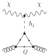
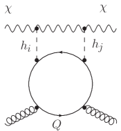
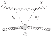
Note that the sum in the first term of Eq. (4.60) only extends over the light quarks. The leading-order gluon interaction with two VDM particles is mediated by one of the two Higgs bosons which couple to the external gluons through a heavy quark triangle diagram, cf. Fig. 2. The charm, bottom and top quark masses are larger than the energy scale relevant for DM direct detection and should therefore be integrated out for the description of the interaction at the level of the nucleon. By calculating the heavy quark triangle diagrams and then integrating out the heavy quarks we obtain the related operator in the heavy quark limit. This is equivalent to calculating the diagram in Fig. 3 with heavy quarks $Q=c,b,t$, and replacing the resulting tensor structure $m_{Q}\bar{Q}Q$ with the effective gluon operator as follows [52, 13, 12]

$$m_{Q}\bar{Q}Q\rightarrow-\frac{\alpha_{S}}{12\pi}G_{\mu\nu}^{a}G^{a\mu\nu}\,,$$ (4.62)

corresponding to the effective leading-order VDM-gluon interaction in Eq. 4.57.

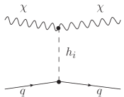
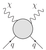
For the tree-level contribution to the SI cross section the $t$-channel diagrams depicted in Fig. 3 have to be calculated for vanishing momentum transfer. The respective Wilson coefficient for the effective operator in Eq. 4.56 is extracted by projecting onto the corresponding tensor structure, $m_{q}q\bar{q}$. Accounting for the additional symmetry factor of the amplitude, this yields finally the following $f_{q}$ factor for the quarks,

$$f_{q}=\frac{1}{2}\frac{gg_{\chi}}{m_{W}}\frac{\sin(2\alpha)}{2}\frac{m_{h_{1}}^{2}-m_{h_{2}}^{2}}{m_{h_{1}}^{2}m_{h_{2}}^{2}}m_{\chi}\,,\quad q=u,d,s,c,b,t\,.$$ (4.63)

As explained above, the heavy quarks $Q=b,c,t$ contribute to the effective gluon interaction. By using Eq. (4.62), the Wilson coefficient for the gluon interaction, $f_{G}$, can be expressed in terms of $f_{q}$ for $q=c,b,t$,

$$f_{G}=\sum_{q=c,b,t}-\frac{\alpha_{S}}{12\pi}f_{q}\;,$$ (4.64)

resulting in the SI LO cross section

$$\sigma^{\text{LO}}=\frac{\sin^{2}2\alpha}{4\pi}\left(\frac{m_{\chi}m_{N}}{m_{\chi}+m_{N}}\right)^{2}\frac{\left(m_{h_{1}}^{2}-m_{h_{2}}^{2}\right)^{2}}{m_{h_{1}}^{4}m_{h_{2}}^{4}}\,\,\frac{m_{\chi}^{2}m_{N}^{2}}{v^{2}v_{S}^{2}}\,\left|\sum_{q=u,d,s}f^{N}_{T_{q}}+3\cdot\frac{2}{27}f^{N}_{T_{G}}\right|^{2}\,.$$ (4.65)

The twist-2 operator does not contribute at LO. The obtained result is in agreement with Ref. [20].

Figure 3: Generic tree-level diagram contribution to the SI cross section. The mediator $S$ corresponds to the two Higgs bosons $h_{1}$ and $h_{2}$. The quark line $q$ corresponds to all quarks $q=u,d,s,c,b,t$.

5 Dark Matter Direct Detection at One-Loop Order

As a next step, we want to include the NLO EW corrections in the calculation of the SI cross section. For this, we evaluate the one-loop contributions to the Wilson coefficients $f_{q}$ and $f_{G}$ in front of the operators in Eq. 4.57. At this order, also the Wilson coefficient $g_{q}$ is non-zero. The additional topologies contributing at NLO EW are depicted in Fig. 4.

(a) Vertex Corrections

(b) Mediator Corrections

(c) Box Corrections

Figure 4: Generic one-loop corrections to the scattering of VDM with the nucleon. The grey blob corresponds to the renormalized one-loop corrections. The corrections can be separated into vertex (a), mediator (b) and box corrections (c).

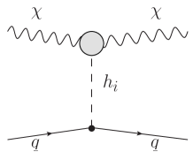
Note that we do not include vertex corrections to the $h_{i}\bar{q}q$ vertex. They are partly given by the nuclear matrix elements and beyond the scope of our study. For the purpose of our investigation, we assume them to be encoded in the effective coupling factors of the respective nuclear matrix elements. In the following, we present the calculation of each topology separately.

5.1 Vertex Corrections $\chi\chi h_{i}$

The effective one-loop coupling $\chi\chi h_{i}$ is extracted by considering loop corrections to the coupling $\chi\chi h_{i}$, where we take the DM particles to be on-shell and assume a vanishing momentum for the Higgs boson $h_{i}$. The amplitude for the NLO vertex including the polarisation vectors $\varepsilon^{(*)}$ of the external VDM particles, is given by

$$\mathit{i}\mathcal{A}_{\chi\chi h_{i}}^{\text{NLO}}=\mathit{i}\mathcal{A}_{\chi\chi h_{i}}^{\text{LO}}+\mathit{i}\mathcal{A}_{\chi\chi h_{i}}^{\text{VC}}+\mathit{i}\mathcal{A}_{\chi\chi h_{i}}^{\text{CT}}\,,$$ (5.66)

with the leading-order amplitude $\mathit{i}\mathcal{A}_{\chi\chi h_{i}}^{\text{LO}}$, the virtual vertex corrections $\mathit{i}\mathcal{A}_{\chi\chi h_{i}}^{\text{VC}}$ and the vertex counterterm $\mathit{i}\mathcal{A}_{\chi\chi h_{i}}^{\text{CT}}$. Denoting by $p$ the four-momentum of the incoming VDM particle, the tree-level amplitude is given by

$$\mathit{i}\mathcal{A}_{\chi\chi h_{i}}^{\text{LO}}=g_{\chi\chi h_{i}}\varepsilon(p)\cdot\varepsilon^{*}(p)=2g_{\chi}m_{\chi}\varepsilon(p)\cdot\varepsilon^{*}(p)\begin{cases}\sin\alpha\,,\quad i=1\\ \cos\alpha\,,\quad i=2\end{cases}\,.$$ (5.67)

The vertex counterterm amplitudes for $i=1,2$ read

$$\mathit{i}\mathcal{A}^{\text{CT}}_{\chi\rightarrow\chi h_{1}}=\left[\frac{1}{2}\left(g_{\chi\chi h_{2}}\delta Z_{h_{2}h_{1}}+g_{\chi\chi h_{1}}\delta Z_{h_{1}h_{1}}\right)+g_{\chi\chi h_{1}}\delta Z_{\chi\chi}+\delta g_{\chi\chi h_{1}}\right]\varepsilon(p)\cdot\varepsilon^{*}(p)$$ (5.68a)

$$\mathit{i}\mathcal{A}^{\text{CT}}_{\chi\rightarrow\chi h_{2}}=\left[\frac{1}{2}\left(g_{\chi\chi h_{1}}\delta Z_{h_{1}h_{2}}+g_{\chi\chi h_{2}}\delta Z_{h_{2}h_{2}}\right)+g_{\chi\chi h_{2}}\delta Z_{\chi\chi}+\delta g_{\chi\chi h_{2}}\right]\varepsilon(p)\cdot\varepsilon^{*}(p)\,,$$ (5.68b)

with the counterterms $\delta g_{\chi\chi h_{i}}$ ($i=1,2$) for the couplings

$$g_{\chi\chi h_{1}} = 2g_{\chi}m_{\chi}\sin\alpha$$ (5.69)

$$g_{\chi\chi h_{2}} = 2g_{\chi}m_{\chi}\cos\alpha$$ (5.70)

derived from

$$\delta g_{\chi\chi h_{i}}=\sum_{p}\frac{\partial g_{\chi\chi h_{i}}}{\partial p}\,,\quad p\in\{m_{\chi},g_{\chi},\alpha\}\,.$$ (5.71)

[5pt]$S=\{h_{i},G_{\chi}\}$   [5pt]$S,V=\{h_{i},G_{\chi}\},\{X\}$   [5pt]$S,V=\{h_{i},G_{\chi}\},\{X\}$   [5pt]$S,V=\{h_{i}\},\{X\}$   
[5pt]$S,V=\{h_{i}\},\{X\}$   [5pt]$S,V=\{h_{i}\},\{X\}$   [5pt]$S,V=\{h_{i}\},\{X\}$   [5pt]$S=\{h_{i},G_{\chi}\}$

Figure 5: Generic diagrams contributing to the virtual corrections to the vertex $\chi\chi h_{i}$. The generic symbols denote $F$ fermions, $S$ scalars and $V$ gauge bosons.

In Fig. 5 all contributing NLO diagrams are shown, where $S$ denotes scalars, $F$ fermions and $V$ vector bosons. At NLO an additional tensor structure arises in the amplitude. Let $p_{\text{in}}$ be the incoming momentum and $p_{\text{out}}$ the outgoing momentum of the DM vector gauge boson. Assuming zero momentum transfer is equivalent to assuming $p_{\text{in}}=p_{\text{out}}$. Note that this assumption is stricter than simply assuming $p_{\text{in}}^{2}=p_{\text{out}}^{2}$, since this only implies the same masses for the incoming and outgoing particles. The additional new tensor structure (denoted by $\sim$ NLO) is given by

$$\mathit{i}\mathcal{A}^{\text{NLO}}=\left(\dots\right)\underbrace{\varepsilon(p_{\text{in}})\cdot\varepsilon^{*}(p_{\text{out}})}_{\sim\text{LO}}+\left(\dots\right)\underbrace{\left(p_{\text{in}}\cdot\varepsilon^{*}(p_{\text{out}})\right)\left(p_{\text{out}}\cdot\varepsilon(p_{\text{in}})\right)}_{\sim\text{NLO}}\,.$$ (5.72)

The additional NLO tensor structure vanishes by assuming $p_{\text{in}}=p_{\text{out}}$, and because for freely propagating gauge bosons we have $\varepsilon(p)\cdot p=0$. The counterterms in Eq. 5.68 cancel all UV-poles of the virtual vertex corrections in Fig. 5 which has been checked both analytically and numerically. Accounting for the symmetry factor of the amplitude and projecting onto the corresponding tensor structure, the vertex corrections are plugged in the generic diagram in Fig. 4(a) which contributes to the operator $\chi_{\mu}\chi^{\mu}m_{q}\bar{q}q$. We will refer to the resulting contribution as $f_{q}^{\text{vertex}}$. Since the expression it quite lengthy, we do not give the explicit formula here.

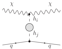
5.2 Mediator Corrections

We proceed in a similar way for the mediator corrections. We calculate the self-energy corrections to the two-point functions with all possible combinations of external Higgs fields and plug these into the one-loop propagator in the generic amplitude in Fig. 4(b). The self-energy contribution to the $h_{i}h_{j}$ propagator ($i,j=1,2$) reads

$$\Delta_{h_{i}h_{j}}=-\frac{\hat{\Sigma}_{h_{i}h_{j}}(p^{2}=0)}{m_{h_{i}}^{2}m_{h_{j}}^{2}}\;,$$ (5.73)

with the renormalised self-energy matrix

$$\begin{pmatrix}\hat{\Sigma}_{h_{1}h_{1}}&\hat{\Sigma}_{h_{1}h_{2}}\\ \hat{\Sigma}_{h_{2}h_{1}}&\hat{\Sigma}_{h_{2}h_{2}}\end{pmatrix}\equiv\hat{\Sigma}(p^{2})=\Sigma(p^{2})-\delta m^{2}-\delta T+\frac{\delta Z}{2}\left(p^{2}-\mathcal{M}^{2}\right)+\left(p^{2}-\mathcal{M}^{2}\right)\frac{\delta Z}{2}\,,$$ (5.74)

where the mass matrix $\mathcal{M}$ and the tadpole counterterm matrix $\delta T$ are defined in Eq. 3.27. The $Z$-factor matrix $\delta Z$ corresponds to the matrix with the components $\delta Z_{h_{i}h_{j}}$ defined in Eq. 3.34. Projecting the resulting one-loop correction on the corresponding tensor structure, we obtain the effective one-loop correction to the Wilson coefficient of the operator $\chi_{\mu}\chi^{\mu}m_{q}\bar{q}q$ induced by the mediator corrections as

$$f_{q}^{\text{med}}=\frac{gg_{\chi}m_{\chi}}{2m_{W}}\sum_{i,j}R_{\alpha,i2}R_{\alpha,j1}\Delta_{h_{i}h_{j}}\,,$$ (5.75)

with the rotation matrix $R_{\alpha}$ defined in Eq. 2.8.

5.3 Box Corrections

[5pt]$F,S=\{q\},\{h_{i}\}$   [5pt]$F,S=\{q\},\{h_{i},G_{\chi}\}$   [5pt]$F,S,V=\{q\},\{h_{i},G_{\chi}\},\{X\}$   [5pt]$F,S=\{q\},\{h_{i}\}$   [5pt]$F,S,V=\{q\},\{h_{i},G_{\chi}\},\{X\}$

Figure 6: Generic diagrams of the box topology contributing to the SI cross section. The symbol $S$ denotes scalars, $F$ fermions and $V$ vector bosons. The flavour of the fermion $F$ and the external quark $q$ are the same as we set the CKM matrix equal to the unit matrix.

We now turn to the box corrections. The generic set of diagrams representative of the box topology is depicted in Fig. 6. In the following, we present the treatment of box diagrams contributing to the SI cross section. In order to extract for the spin-independent cross section the relevant tensor structures from the box diagram, we expand the loop diagrams in terms of the momenta $p_{q}$ of the external quark that is not relativistic [12]. Since we are considering zero momentum transfer, the incoming and outgoing momenta of the quark are the same,

$$p_{q}^{\text{in}}=p_{q}^{\text{out}}\,.$$ (5.76)

Note that as in the case of the vertex corrections this requirement is stricter than requiring that the squared momenta are the same, since this only implies same masses for incoming and outgoing particles. Assuming small quark momenta, and because the mass of the light quarks is much smaller than the energy scale of the interaction, allows for the simplification of the propagator terms arising in the box diagrams through the expansion,

$$\frac{1}{(l\pm p_{q})^{2}-m_{q}^{2}}=\frac{1}{l^{2}}\mp\frac{2p_{q}\cdot l}{l^{4}}+\mathcal{O}(p_{q}^{2}/l^{4})\,,$$ (5.77)

where $l$ is the loop momentum of the box diagram, $m_{q}$ the mass of the quark and where we use $m_{q}^{2}=p_{q}^{2}$. After applying this expansion to the box diagrams, the result has to be projected onto the required tensor structures contributing to the operators in Eq. 4.57. The box diagrams contribute to $X_{\mu}X^{\mu}m_{q}\bar{q}q$ and the twist-2 operators. By rewriting[13, 50, 51]

$$\bar{q}\mathit{i}\partial_{\mu}\gamma_{\nu}q=\mathcal{O}_{\mu\nu}^{q}+\bar{q}\frac{\mathit{i}\partial_{\mu}\gamma_{\nu}-\mathit{i}\partial_{\nu}\gamma_{\mu}}{2}q+\frac{1}{4}g_{\mu\nu}m_{q}\bar{q}q\,,$$ (5.78)

the parts of the loop amplitude that correspond to the twist-2 and the $X_{\mu}X^{\mu}m_{q}\bar{q}q$ operator can be extracted. The asymmetric part in Eq. 5.78 does not contribute to the SI cross section and therefore can be dropped. We refer to these one-loop contributions to the corresponding tree-level Wilson coefficients as $f_{q}^{\text{box}}$ and $g_{q}^{\text{box}}$.

As discussed in Refs. [13, 12] the box diagrams also induce additional contributions to the effective gluon interaction with the VDM particle that have to be taken into account in the Wilson coefficient $f_{G}$ in Eq. (4.57b). The naive approach of using the same replacement as in Eq. 4.62 to obtain the gluon interaction induces large errors [12]. To circumvent the over-estimation of the gluon interaction without performing the full two-loop calculation, we adopt the ansatz proposed in Ref. [13]. For heavy quarks compared to the mediator mass, it is possible to derive an effective coupling between two Higgs bosons and the gluon fields. Using the Fock-Schwinger gauge allows us to express the gluon fields in terms of the field strength tensor $G^{a}_{\mu\nu}$, simplifying the extraction of the effective two-loop contribution to $f_{G}$. Integrating out the top-quark yields the following effective two-Higgs-two-gluon coupling[13]

$$\mathcal{L}^{hhGG}=\frac{1}{2}d_{G}^{\text{eff}}h_{i}h_{j}\frac{\alpha_{S}}{12\pi}G^{a}_{\mu\nu}G^{a\,\mu\nu}\,,$$ (5.79)

where the effective coupling $d_{G}^{\text{eff}}$ of Ref. [13] has to be adopted to our model. First of all we only have scalar-type mediators, given by the Higgs bosons $h_{i}$, so that the mixing angle $\phi_{\text{SM}}$ of Ref. [13] which quantifies the CP-odd admixture, is set to

$$\phi_{\text{SM}}=0\,.$$ (5.80)

Second, the coupling of the Higgs bosons $h_{i}$ to the top quark differs depending on which Higgs boson is coupled, so that the effective coupling in Eq. 5.79 becomes

$$d_{G}^{\text{eff}}\to\left(d_{G}^{\text{eff}}\right)_{ij}=(R_{\alpha})_{i1}(R_{\alpha})_{j1}\frac{1}{v^{2}}\,,$$ (5.81)

with the rotation matrix $R_{\alpha}$ defined in Eq. 2.8. The effective coupling allows for the calculation of the box-type diagram in Fig. 7 (right).

Figure 7: The full two-loop gluon interaction with the DM candidate (left) and the effective two-loop interaction after integration out the heavy quarks (right).

In Ref. [13], the full two-loop calculation was performed. The comparison with the complete two-loop result showed very good agreement between the approximate and the exact result for mediator masses below $m_{t}$. Our model is structurally not different in the sense that the mediator coupling to the DM particle (a fermion in Ref. [13]) is also a scalar particle so that the results obtained in Ref. [13] should be applicable to our model as well. Moreover, the box contribution to the NLO SI direct detection cross section is only minor as we verified explicitly.

The diagram in Fig. 7 (right) yields the following contribution to the Lagrangian

$$\mathcal{L}_{\text{eff}}\supset\left(d_{G}^{\text{eff}}\right)_{ij}C^{ij}_{\triangle}\chi_{\mu}\chi^{\mu}\frac{-\alpha_{S}}{12\pi}G^{a}_{\mu\nu}G^{a\,\mu\nu}\,,$$ (5.82)

where $C^{ij}_{\triangle}$ denotes the contribution from the triangle loop built up by $h_{i}$, $h_{j}$ and the VDM particle. It has to be extracted from the calculated amplitude of Fig. 7 (right). Using Eq. 4.57b the contributions by the box topology to the gluon-DM interaction are given by

$$f_{G}^{\text{top}}=\left(d_{G}^{\text{eff}}\right)_{ij}C^{ij}_{\triangle}\frac{-\alpha_{S}}{12\pi}\,.$$ (5.83)

5.4 The SI One-Loop Cross Section

In the last sections we discussed the extraction of the one-loop effective form factors for the operators in Eq. 4.57. The NLO EW SI cross section can then be obtained by using the effective one-loop form factor

$$\frac{f_{N}^{\text{NLO}}}{m_{N}}=\sum_{q=u,d,s}f_{q}^{\text{NLO}}f^{N}_{T_{q}}+\sum_{q=u,d,s,c,b}\frac{3}{4}\left(q(2)+\bar{q}(2)\right)g_{q}^{\text{NLO}}-\frac{8\pi}{9\alpha_{S}}f^{N}_{T_{G}}f_{G}^{\text{NLO}}\,,$$ (5.84)

with the Wilson coefficients at one-loop level given by

$$f_{q}^{\text{NLO}}=f_{q}^{\text{vertex}}+f_{q}^{\text{med}}+f_{q}^{\text{box}}$$ (5.85a)

$$g_{q}^{\text{NLO}}=g_{q}^{box}$$ (5.85b)

$$f_{G}^{\text{NLO}}=-\frac{\alpha_{S}}{12\pi}\sum_{q=c,b,t}\left(f_{q}^{\text{vertex}}+f_{q}^{\text{med}}\right)+f_{G}^{\text{top}}\,.$$ (5.85c)

Like at LO, the heavy quark contributions of $f_{q}^{\text{vertex}}$ and $f_{q}^{\text{med}}$ have to be attributed to the effective gluon interaction. With the LO form factor given by

$$\frac{f_{N}^{\text{LO}}}{m_{N}}=f_{q}^{\text{LO}}\left[\sum_{q=u,d,s}f^{N}_{T_{q}}+\sum_{q=c,b,t}\frac{2}{27}f_{T_{G}}^{N}\right]\,,$$ (5.86)

where $f_{q}^{\text{LO}}$ has been given in Eq. (4.63), we have for the NLO EW SI cross section at leading order in $\alpha_{S}$,

$$\sigma_{N}=\frac{1}{\pi}\left(\frac{m_{N}}{m_{\chi}+m_{N}}\right)^{2}\left[|f_{N}^{\text{LO}}|^{2}+2\mbox{Re}\left(f_{N}^{\text{LO}}f_{N}^{\text{NLO}*}\right)\right]\;.$$ (5.87)

6 Numerical Analysis

In our numerical analysis we use parameter points that are compatible with current theoretical and experimental constraints. These are obtained by performing a scan in the parameter space of the model and by checking each data set for compatibility with the constraints. In order to do so, the VDM model was implemented in the code ScannerS [53, 54] which automatises the parameter scan. We require the SM-like Higgs boson (denoted by $h$ in the following) to have a mass of $m_{h}=125.09$ GeV [55]. With ScannerS, we check if the minimum of the potential is the global one and if the generated points satisfy the theoretical constraints of boundedness from below and perturbative unitarity. We furthermore impose the perturbativity constraint $g_{\chi}^{2}<4\pi$. Furthermore, the model has to comply with the experimental Higgs data. In the VDM model, the Higgs couplings to the SM particles are modified by a common factor given in terms of the mixing angle $\alpha$, that is hence constrained by the combined values for the signal strengths [55]. Through an interface with HiggsBounds [56, 57, 58] we additionally check for collider bounds from LEP, Tevatron and the LHC. We require agreement with the exclusion limits derived for the non-SM-like Higgs boson at 95% confidence level. Among these searches the most stringent bound arises from the search for heavy $ZZ$ resonances [59]. Still, the bounds for the mixing angle $\alpha$ derived from the measurement of the Higgs couplings are by far the most relevant. In order to check for the constraints from the Higgs data, the Higgs decay widths and branching ratios were calculated with sHDECAY [54], which includes the state-of-the-art higher-order QCD corrections. The code sHDECAY is based on the implementation of the models in HDECAY [60, 61].

Concerning the DM constraints, information on the DM particle from LHC searches through the invisible width of the SM Higgs boson were taken into account [56, 57, 58]. Furthermore, the DM relic abundance has been calculated with MicrOMEGAs [62, 63, 64, 65], and compared with the current experimental result from the Planck Collaboration [66],

$$({\Omega}h^{2})^{\rm obs}_{\rm DM}=0.1186\pm 0.002\;.$$ (6.88)

We do not force the DM relic abundance to be in this interval, but rather require the calculated abundance to be equal to or smaller than the observed one. Hence, we allow the DM to not saturate the relic density and therefore define a DM fraction

$$f_{\chi\chi}=\frac{({\Omega}h^{2})_{\chi}}{(\Omega h^{2})^{\rm obs}_{\text{DM}}}\,,$$ (6.89)

where $(\Omega h^{2})_{\chi}$ stands for the calculated DM relic abundance of the VDM model. DM indirect detection also provides constraints on the VDM model. The annihilation into visible states, mainly into $ZZ$, $W^{+}W^{-}$, $b\bar{b}$ and light quark pairs, can be measured by Planck [66], if it manifests itself in anisotropies of the cosmic microwave background (CMB), by Fermi-LAT [67] if it comes form the $\gamma$-ray signals in the spheroidal dwarf galaxies, and by AMS-02 [68, 69] if it originates from $e^{\pm}$ excesses in the Milky Way. As shown in Ref. [70], the Fermi-LAT upper bound on the DM annihilations is the most stringent one. In order to obtain the bound, we follow Ref. [67] in their claim that all final states give approximately the same upper bound on the DM annihilation cross sections. Hence we use the Fermi-LAT bound from Ref. [67] on $b\bar{b}$ when $m_{\chi}\geqslant m_{b}$, and on light quarks for $m_{\chi}<m_{b}$. In the comparison with the data, the DM fraction in Eq. (6.89) has to be taken into account, and an effective DM annihilation cross section is defined by

$$\sigma^{\rm eff}_{\chi\chi}=f^{2}_{\chi\chi}\sigma_{\chi\chi}\;,$$ (6.90)

with $f_{\chi\chi}$ and $\sigma_{\chi\chi}$ computed by MicrOMEGAs.

The sample was generated taking into account the experimental bounds on the DM nucleon SI cross section at LO. The most stringent bound on this cross section is the one from the XENON1T [71, 72] experiment. We apply the latest XENON1T upper bounds [72] for a DM mass above 6 GeV and the combined limits from CRESST-II [73] and CDMSlite [74] are used for lighter DM particles. Note that the experimental limits on DM-nucleon scattering were derived by assuming that the DM candidate makes up for all of the DM abundance. Hence, the correct quantity to be directly compared with experimental limits is the effective DM-nucleon cross-section defined by

$$\sigma^{\rm eff}_{\chi N}\equiv f_{\chi\chi}\sigma_{\chi N}\;,$$ (6.91)

where $\chi N$ stands for the scattering VDM $\chi$ with the nucleon $N$, and $f_{\chi\chi}$ denotes the respective DM fraction, defined in Eq. (6.89). The formula for the LO direct detection cross section $\sigma_{\chi N}$ in our VDM model has been given in Eq. (4.65) and the NLO contributions have been discussed in Section 5. For our numerical analysis, we use the LO and NLO results for $N=p$.

The ranges of the input parameters of the scan performed to generate viable parameter sets are listed in Table 1. From here on, we denote the non-SM-like of the two CP-even Higgs bosons $m_{h_{i}}$ ($i=1,2$) by $m_{\phi}$, the SM-like Higgs boson is called $m_{h}$. Note, that in ScannerS the scan is performed over $m_{\chi}$ and $v_{S}$ instead of $m_{\chi}$ and $g_{\chi}$. The corresponding $g_{\chi}$ values are given by $g_{\chi}=m_{\chi}/v_{S}$. Only points with $g_{\chi}^{2}\leq 4\pi$ are retained. Note that we vary $\alpha$ in the range $[-\pi/4,\pi/4]$ to optimize the scan. This is possible due to the bound on $\sin\alpha$ that comes from the combined signal strength measurements of the production and decay of the SM-like Higgs boson [55].

	$m_{\phi}$ [GeV]	$m_{\chi}$ [GeV]	$v_{S}$ [GeV]	$\alpha$
min	1	1	1	$-\frac{\pi}{4}$
max	1000	1000	$10^{7}$	$\frac{\pi}{4}$

Table 1: Input parameters for the VDM model scan, all parameters varied independently between the given minimum and maximum values. The SM-like Higgs boson mass is set $m_{h}=125.09$ GeV and the SM VEV $v=246.22$ GeV.

The remaining input parameters, gauge, lepton and quark masses, electric coupling, Weinberg angle and weak $SU(2)$ coupling, are set to

$$\begin{array}[]{lllllllll}m_{W}&=&80.398\mbox{ GeV }\;,&m_{Z}&=&91.1876\mbox{ GeV }\;,&\sin\theta_{W}&=&0.4719\;,\\ m_{e}&=&0.511\cdot 10^{-3}\mbox{ GeV }\;,&m_{\mu}&=&0.1057\mbox{ GeV }\;,&m_{\tau}&=&1.777\mbox{ GeV }\;,\\ m_{u}&=&0.19\mbox{ MeV }\;,&m_{d}&=&0.19\mbox{ MeV }\;,&m_{s}&=&0.19\mbox{ MeV }\;,\\ m_{c}&=&1.4\mbox{ GeV }\;,&m_{b}&=&4.75\mbox{ GeV }\;,&m_{t}&=&172.5\mbox{ GeV }\;.\end{array}$$ (6.96)

For the proton mass we take

$$m_{p}=0.93827\mbox{ GeV}\,.$$ (6.97)

6.1 Results

In the following we present the LO and NLO results for the spin-independent direct detection cross section of the VDM model. We investigate the size of the NLO corrections and their phenomenological impact. We furthermore discuss the gauge dependence of the results and the influence of the renormalisation scheme on the NLO results. If not stated otherwise, results are presented for the Feynman gauge, i.e. the gauge parameter $\xi$ is set equal to one, $\xi=1$. In the NLO results, the default renormalisation scheme for the mixing angle $\alpha$ is the KOSY scheme, cf. Subsection 3.2.

6.1.1 The SI Direct Detection Cross Section at Leading Order

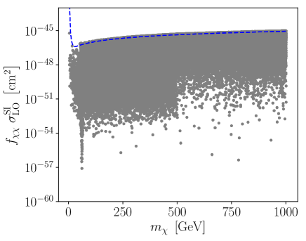
In Fig. 8 we show in grey the LO results of the direct detection cross section for all points of the VDM model that are compatible with our applied constraints, as a function of the DM mass $m_{\chi}$. Note, that we also include the perturbativity limit on $g_{\chi}$, $g_{\chi}^{2}<4\pi$. The result is compared to the Xenon limit shown in blue. Note that, in order to be able to compare with the Xenon limit, we applied the correction factor $f_{\chi\chi}$ to the LO and NLO direct detection cross section, cf. Eq. (6.91). Since the compatibility with the Xenon limit is already included in the selection of valid parameter points, all cross section values lie below the blue line (modulo the size of the grey points). As can be inferred from Fig. 8, the LO cross section can be substantially smaller than the present sensitivity of the Xenon experiment, by more than 10 orders of magnitude.

Figure 8: Grey: The tree-level SI cross section $\sigma^{\text{LO}}$ versus the DM mass $m_{\chi}$ in GeV for the complete parameter sample compatible with the applied constraints. The blue line denotes the Xenon Limit.

6.1.2 Results for $m_{\phi}<m_{t}$

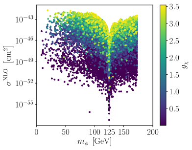
We now investigate the dependence of the LO and NLO direct detection cross section on $g_{\chi}$ and the size of the NLO corrections for the parameter sets featuring a non-SM-like Higgs boson with a mass $m_{\phi}<m_{t}$. For these, the approximate treatment of the NLO box contributions discussed in Subsection 5.3 can be applied. In Fig. 9 we display for all parameter sets passing our constraints that additionally feature $m_{\phi}<m_{t}$ the LO direct detection cross section in the left panel and the NLO result in the right panel, as a function of $m_{\phi}$. The color code quantifies the coupling $g_{\chi}\leq\sqrt{4\pi}$. Note, that here and in the following we do not apply the correction factor $f_{\chi\chi}$ Eq. (6.89) on the direct detection limit, as long as we do not directly compare with the Xenon limit. This is why the LO cross section in Fig. 9 is larger than in Fig. 8.

Figure 9: Spin-independent direct detection LO cross section (left) and NLO cross section (right) versus the mass $m_{\phi}$ for the parameter sample passing all constraints and $m_{\phi}<m_{t}$. The color code denotes the size of the dark gauge coupling $g_{\chi}$.

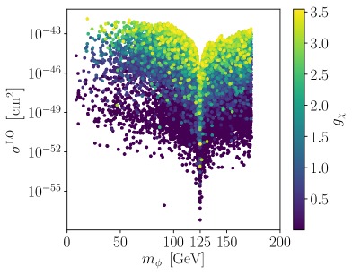
Both the LO and the NLO contribution to the SI direct detection cross section are proportional to $f_{q}^{\text{LO}}$ and therefore proportional to $g_{\chi}$, $\sin 2\alpha$ and $(m_{h_{1}}^{2}-m_{h_{2}}^{2})\equiv(m_{h}^{2}-m_{\phi}^{2})$. This behaviour is reflected in Fig. 9. We observe that the LO cross section increases with $g_{\chi}$, more specifically $g_{\chi}^{2}$ (yellow points) and drops for $m_{\phi}=m_{h}=125.09$ GeV. The NLO corrections on the other hand increase with $g_{\chi}^{3}$. The reason is that, as we explicitly verified, the NLO corrections are dominated by the vertex corrections. The vertex corrections are proportional to $g_{\chi}^{2}$, so that the NLO contribution to the cross section scales as $2\,\mbox{Re}(f_{q}^{\text{LO}}f_{q}^{\text{vertex}*})\propto g_{\chi}^{3}$, in contrast to the LO contribution that is proportional to $g_{\chi}^{2}$. In total the $K$-factor, i.e. the ratio between NLO and LO cross section, therefore increases with $g_{\chi}$.

Being proportional to $f_{q}^{\text{LO}}$ the NLO corrected cross section also drops for $m_{\phi}=m_{h}$, so that the sensitivity of the direct detection experiment is not increased after inclusion of the NLO corrections; the blind spots remain also at NLO. In our scan we furthermore did not find any parameter points where a specific parameter combination leads to an accidental suppression at LO that is removed at NLO. There is a further blind spot when $\alpha=0$. However, in this case the SM-like Higgs boson has exactly SM-like couplings and the new scalar decouples from all SM particles except for the coupling with the SM-like Higgs boson. In this scenario the SM-like Higgs decouples from the vector dark matter particle, and, depending on the mass of the second scalar and its coupling strength with the SM-like Higgs boson, we may end up with two dark matter candidates with the second scalar being metastable. The study of such a scenario is beyond the scope of this paper and we do not consider this case further here.

Figure 10: $K$-factor versus the Higgs mass $m_{\phi}$ (left) and $\sigma^{\text{LO}}$ (right) for the parameter sample passing all constraints and $m_{\phi}<m_{t}$. The color code denotes the size of the dark gauge coupling $g_{\chi}$.

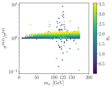
The $K$-factor is depicted in Fig. 10, as a function of $m_{\phi}$ (left) and $\sigma^{\text{LO}}$ (right). The colour code indicates the size of $g_{\chi}$. The $K$-factor is mostly positive and the bulk of $K$-facture values ranges between 1 and about 2.3. As mentioned above, the $K$-factor increases with $g_{\chi}$, as can also be inferred from the figure, in particular from Fig. 10 (right).

In this and all other plots, we excluded points with $m_{\phi}\approx m_{h}$ and $K$-factors where $|K|>2.5$. We found that for $m_{\phi}\approx m_{h}$ the interference effects between the $h$ and $\phi$ contributions, that become relevant here, largely increase the (dominant) vertex contribution $f_{q}^{\text{vertex}}$ to the effective NLO form factor. It exceeds by far the LO form factor $f_{q}^{\text{LO}}$. Depending on the sign of $f_{q}^{\text{vertex}}$, the NLO cross section, which is proportional to $2\,\mbox{Re}(f_{q}^{\text{LO}}f_{q}^{\text{vertex}*})$, is largely increased or suppressed, inducing for large negative NLO amplitudes negative NLO cross sections. In these regions, the NLO results are therefore no longer reliable. Two-loop contributions might lead to a better perturbative convergence, but are beyond the scope of this paper. We deliberately did not take into account one-loop squared terms to remove the negative cross sections. Such an approach would only include parts of the two-loop contributions. Whether or not they approximate the total two-loop results well enough can only be judged after performing the complete two-loop calculation. This is why we chose the conservative approach to exclude these points from our analysis.

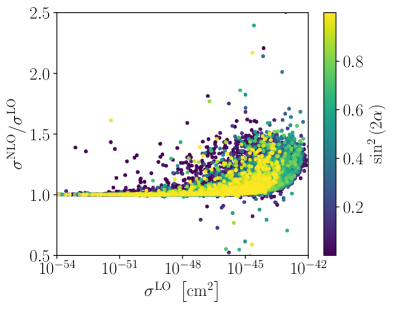
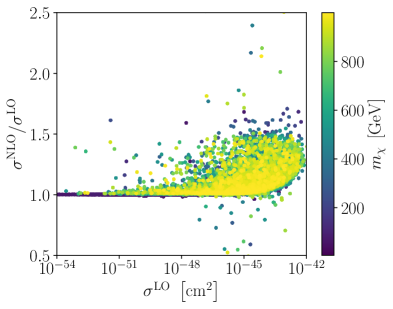
In Fig. 11, we show the $K$-factor as function of $\sigma^{\text{LO}}$, but with the colour code indicating the size of $\sin^{2}2\alpha$ (left) and $m_{\chi}$ right. There is no clear correlation between the $K$-factor and $\sin^{2}2\alpha$ or $m_{\chi}$. These plots furthermore show, that there is no correlation between the maximum size of $\sigma^{\text{LO}}$ and $m_{\chi}$ or $\sin^{2}2\alpha$, while the maximum $\sigma^{\text{LO}}$ values require large $g_{\chi}$ values, cf. Fig. 10 (right).

Figure 11: $K$-factor as function of the LO direct detection cross section with the color code indicating the size of $\sin^{2}2\alpha$ (left) and $m_{\chi}$ (right).

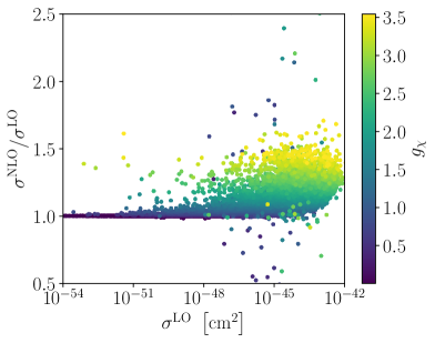
6.1.3 Results for $m_{\phi}>m_{t}$

We now turn to the parameter region of our sample of valid points where the approximation described in Subsection 5.3 is a priori not valid. We cannot judge the goodness of the approximation in this parameter region without doing the full two-loop calculation which is beyond the scope of this paper. We can check, however, if we see some unusual behaviour compared to the results for parameter sets with $m_{\phi}<m_{t}$, where the approximation can be applied.

Figure 12: $K$-factor versus the LO SI cross section. The color code denotes the size of the dark gauge coupling $g_{\chi}$ for the parameter sample passing all constraints and $m_{\phi}>m_{t}$.

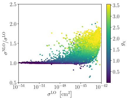
Figure 12 shows the $K$-factor as a function of the LO SI direct detection cross section. The size of $g_{\chi}$ is indicated by the color code. We only take into account parameter samples compatible with all constraints and where $m_{\phi}>m_{t}$. As already observed and discussed for the parameter sample with $m_{\phi}<m_{t}$, also here the $K$-factor increases with $g_{\chi}$. Overall, the bulk of points reaches larger $K$-factors than for $m_{\phi}<m_{t}$ but remains below 2.5. So, the behaviour of the $K$-factor does not substantially differ from the results for $m_{\phi}<m_{t}$. The comparison of the approximate and exact result in Ref. [13] showed that the difference in the box contribution between the two results does not exceed one order of magnitude for a pseudoscalar mediator with mass 1 TeV and remains small even for scalar mediator masses up to 1 TeV (cf. Fig. 4 in Ref. [13]). Together with the fact that the box contribution makes up only for a small part of the NLO SI direct detection cross section, we conclude that our approximate NLO results for parameter sets with larger mediator masses should also be applicable in this parameter region.

6.1.4 Gauge Dependence

As has been discussed in Ref. [33] for the 2HDM and in Ref. [37] for the N2HDM the renormalisation of the mixing angle $\alpha$ in the KOSY scheme leads to gauge parameter dependent results. We therefore check here the gauge dependence of our NLO results by performing the calculation in the general $R_{\xi}$ gauge and comparing it with our default result in the Feynman gauge $\xi=1$.

We introduce the relative gauge dependence $\Delta_{\xi}\sigma^{\text{NLO}}$, defined as

$$\Delta_{\xi}\sigma^{\text{NLO}}=\left(\sigma^{\text{NLO}}\big{|}_{\xi}-\sigma^{\text{NLO}}\big{|}_{\xi=1}\right)/\sigma^{\text{NLO}}\big{|}_{\xi=1}\;,$$ (6.98)

where $\sigma^{\text{NLO}}\big{|}_{\xi}$ denotes the NLO SI direct detection cross section calculated in the general $R_{\xi}$ gauge and $\sigma^{\text{NLO}}\big{|}_{\xi=1}$ the result in the Feynman gauge. In Fig. 13 we show $\Delta_{\xi}\sigma^{\text{NLO}}$ as a function of the gauge parameter $\xi$, for two sample parameter points of our valid parameter set, called point 5 and 6, respectively. They are given by the following input parameters. For the parameter point 5 we have

$$\begin{array}[]{lllllll}\mbox{\text@underline{Point 5: }}&m_{\phi}&=&283.44\mbox{ GeV }\;,&m_{\chi}&=&914.76\mbox{ GeV }\;,\\ &g_{\chi}&=&7.67\;,&\alpha&=&0.07312\;.\end{array}$$ (6.101)

The parameter point 6 is given by

$$\begin{array}[]{lllllll}\mbox{\text@underline{Point 6: }}&m_{\phi}&=&119.84\mbox{ GeV }\;,&m_{\chi}&=&766.82\mbox{ GeV }\;,\\ &g_{\chi}&=&1.555\;,&\alpha&=&0.425943\;.\end{array}$$ (6.104)

Figure 13: Relative gauge dependence $\Delta_{\xi}\sigma$ versus the gauge parameter $\xi$ for parameter point number 5 (left) and 6 (right). See text, for their definitions.

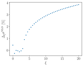
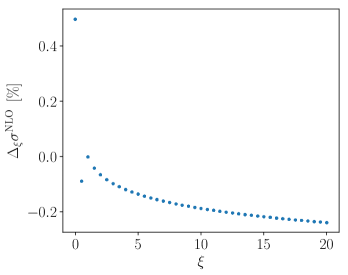
As can be inferred from Fig. 13, we clearly see a gauge dependence of the NLO results. The relative gauge dependence is, however, small with values below the few per cent level for a rather large range of $\xi$ variation. Note also, that a gauge parameter dependence a priori is no problem as long as it is made sure that the explicit value of the gauge parameter is accounted for when interpreting the results.

6.1.5 Renormalisation Scheme Dependence

We now investigate the influence of the renormalisation scheme and scale on the NLO result. For this, we show in Fig. 14 the $K$-factor for the whole data sample passing our constraints for three different renormalisation schemes of the mixing angle $\alpha$ as a function of the LO cross section. The chosen schemes have been described in Subsection 3.2 and are the KOSY scheme (yellow points), the process-dependent scheme (green) and the $\overline{\mbox{MS}}$ scheme (violet). The scale applied in the $\overline{\mbox{MS}}$ scheme is $\mu_{0}=1$ GeV. The KOSY scheme has been shown to lead to a gauge-parameter dependent definition of the counterterm $\delta\alpha$ [33, 37]. This is also the case for the $\overline{\mbox{MS}}$ scheme. As can be inferred from the plot, the $\overline{\mbox{MS}}$ scheme additionally leads to unnaturally large NLO corrections with $K$-factor values up to about $10^{8}$ for our data sample (not shown in the plot). This has been known already from previous investigations in the 2HDM [33] and N2HDM [37]. The process-dependent scheme has the virtue of implying a manifestly gauge-independent definition of the mixing angle counterterm. However, also here the NLO corrections are unacceptably large with values up to about $10^{9}$, so that also this scheme turns out to be unsuitable for practical use. This behaviour has also been observed in our previous works [33, 37]. We therefore conclude that the KOSY scheme should be used in the computation of the NLO corrections. The fact that it is gauge dependent is no problem as long as the chosen gauge is clearly stated when presenting results. Moreover, by applying a pinched scheme, the gauge dependence can be avoided, cf. Ref. [33]. This is left for future work.

Figure 14: The $K$-factor versus the LO SI direct detection cross section for the whole data sample passing all constraints and for three different renormalisation schemes of $\alpha$: the KOSY scheme (yellow), the process-dependent scheme (green), the $\overline{\mbox{MS}}$ scheme (violet).

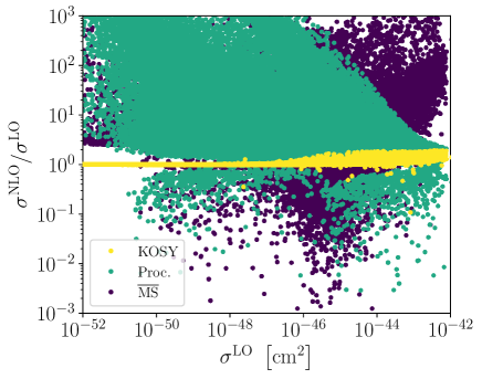
The uncertainty due to missing higher-order corrections can be estimated by varying the renormalisation scheme or by varying the renormalisation scale. The comparison of the KOSY with the other two renormalisation schemes makes no sense as the latter lead to unacceptably large corrections. The KOSY scheme does not allow us to vary the renormalisation scale, so that we cannot provide an estimate of the uncertainty due to missing higher order corrections. We conclude with the remark that the variation of the renormalisation scale between 1/2 and 2 times the scale $\mu_{0}$ in the $\overline{\mbox{MS}}$ scheme leads to a variation of the NLO cross section of about 16% - in contrast to the unphysically large corrections that are to be traced back to the blowing-up of the $\overline{\mbox{MS}}$ counterterm of $\alpha$.

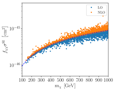
6.1.6 Phenomenological Impact of the NLO Corrections on the Xenon Limit

We now turn to the discussion of the phenomenological impact of our NLO results. In Fig. 15 (left) we show the LO direct detection cross section (blue points) and the NLO result (orange) compared to the Xenon limit (blue-dashed), as a function of the DM particle mass. For the consistent comparison with the Xenon limit we applied the correction factor $f_{\chi\chi}$ (Eq. 6.91) to the LO and NLO cross section in both plots of Fig. 15. In the left figure we plot all parameter points where the LO cross section does not exceed the Xenon limit but the NLO result does. This plot shows that for a sizeable number of parameter points, the compatibility with the experimental constraints would not hold at NLO any more. This demonstrates that the NLO corrections are important and need to be accounted for in order to make reliable predictions about the viable parameter space of the VDM model.

Figure 15: The SI cross section including the correction factor $f_{\chi\chi}$ at LO (biue) and NLO (orange) compared to the Xenon limit (blue-dashed) versus the DM mass $m_{\chi}$. The definition of the parameter sample included in the left and right plots is described in the text.

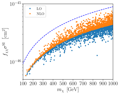
In the right plot we display the same quantities, but only for parameter points of our data sample where

$$\frac{|\sigma_{{\text{Xe}}}(m_{\chi})-\sigma^{\text{LO}}|}{\sigma^{\text{LO}}}>1$$ (6.105)

and

$$\frac{|\sigma_{\text{Xe}}(m_{\chi})-\sigma^{\text{NLO}}|}{\sigma^{\text{NLO}}}<1\;.$$ (6.106)

This implies we only consider parameter points where the LO cross section is much smaller than the Xenon limit, but the NLO cross section is of the order of the Xenon limit. We learn from this figure that although LO results might suggest that the Xenon experiment is not sensitive to the model, this statement does not hold any more when NLO corrections are taken into account. These results confirm the importance of the NLO corrections when interpreting the data.

7 Conclusions

In this paper, we investigated a minimal model with a VDM particle. We computed the NLO corrections to the direct detection cross section for the scattering of the VDM particle off a nucleon. We developed the renormalisation of the model, proposing several renormalisation schemes for the mixing angle $\alpha$ of the two physical scalars of the model. We computed the leading corrections, including relevant two-loop box contributions to the effective gluon interaction in the heavy quark approximation. With the box contributions to the NLO cross section being two orders of magnitude below the leading vertex corrections, we estimated the error induced by the approximation to be small. Interference effects of the two scalar particles that become important for degenerate mass values on the other hand, were found to be large and require further investigations beyond the scope of this paper, namely the computation of the complete two-loop contributions. Outside this region, the perturbative series is well-behaved and $K$-factors of up to about 2.5 were found.

We further investigated the impact of the chosen renormalisation scheme for $\alpha$. While the process-dependent renormalisation of $\alpha$ is manifestly gauge-parameter independent, it was found to lead to unphysically large corrections. This did not improve by choosing the gauge-parameter dependent $\overline{\mbox{MS}}$ scheme. A renormalisation scheme exploiting the OS conditions of the scalar fields on the other hand, leads to moderate $K$-factors, while being manifestly gauge-parameter dependent. For the proper interpretation of the data, therefore, the choice of the gauge parameter has to be specified here.

We found that the NLO corrections can either enhance or suppress the cross section. With $K$-factors of up to about 2.5, they are important for the correct interpretation of the viability of the VDM model based on the experimental limits on the direct detection cross section. The NLO corrections can increase the LO results to values where the Xenon experiment becomes sensitive to the model, or to values where the model is even excluded due to cross sections above the Xenon limit. In case of suppression, parameter points that might be rejected at LO may render the model viable when NLO corrections are included.

The next steps would be to investigate in greater detail the interesting region of degenerate scalar masses and study its implication on phenomenology in order to further be able to delineate the viability of this simple SM extension in providing a VDM candidate.

Acknowledgments

We are thankful to M. Gabelmann, M. Krause and M. Spira for fruitful and clarifying discussions. We are grateful to D. Azevedo for providing us with the data samples. R.S. is supported in part by a CERN grant CERN/FIS-PAR/0002/2017, an FCT grant PTDC/FISPAR/31000/2017, by the CFTC-UL strategic project UID/FIS/00618/2019 and by the NSC, Poland, HARMONIA UMO-2015/18/M/ST2/00518.

Appendix A Nuclear Form Factors

We here present the numerical values for the nuclear form factors defined in Eq. 4.59. The values of the form factors for light quarks are taken from micrOmegas[75]

$$f^{p}_{T_{u}}=0.01513\,,\quad f^{p}_{T_{d}}=0.0.0191\,,\quad f^{p}_{T_{s}}=0.0447\,,$$ (A.107a)

$$f^{n}_{T_{u}}=0.0110\,,\quad f^{n}_{T_{d}}=0.0273\,,\quad f^{n}_{T_{s}}=0.0447\,,$$ (A.107b)

which can be related to the gluon form factors as

$$f^{p}_{T_{G}}=1-\sum_{q=u,d,s}f_{T_{q}}^{p}\,,\qquad f^{n}_{T_{G}}=1-\sum_{q=u,d,s}f_{T_{q}}^{n}\,.$$ (A.108)

The needed second momenta in Eq. 4.59 are defined at the scale $\mu=m_{Z}$ by using the CTEQ parton distribution functions [76],

$$u^{p}(2)=0.22\,,\qquad \bar{u}^{p}(2)=0.034\,,$$ (A.109a)

$$d^{p}(2)=0.11\,,\qquad \bar{d}^{p}(2)=0.036\,,$$ (A.109b)

$$s^{p}(2)=0.026\,,\qquad \bar{s}^{p}(2)=0.026\,,$$ (A.109c)

$$c^{p}(2)=0.019\,,\qquad \bar{c}^{p}(2)=0.019\,,$$ (A.109d)

$$b^{p}(2)=0.012\,,\qquad \bar{b}^{p}(2)=0.012\,,$$ (A.109e)

where the respective second momenta for the neutron can be obtained by interchanging up- and down-quark values.

Appendix B Feynman Rules

In the following we list the Feynman rules needed to perform the one-loop calculation. The Feynman rules are derived by using the program package SARAH [22, 23, 24, 25]. All momentum conventions are adopted from the FeynArts conventions. The trilinear Higgs couplings read

$$\begin{aligned} \hbox{\includegraphics[width=91.04742pt]{hXX}}\end{aligned} =\mathit{i}2g_{\chi}m_{\chi}R_{\alpha,i2}\,,\quad \begin{aligned} \includegraphics[width=91.04742pt]{hZZ}\end{aligned} =\mathit{i}\frac{gm_{Z}^{2}}{m_{W}}R_{\alpha,1i}\,,\quad$$ (B.110a)

$$\begin{aligned} \includegraphics[width=91.04742pt]{hWW}\end{aligned} =\mathit{i}gm_{W}R_{\alpha,1i}\,,\quad \begin{aligned} \includegraphics[width=91.04742pt]{hFF}\end{aligned} =\mathit{i}\frac{gm_{F}}{2m_{W}}R_{\alpha,1i}\,,\quad$$ (B.110b)

$$\begin{aligned} \includegraphics[width=91.04742pt]{hG0G0.pdf}\end{aligned} =-\mathit{i}\frac{g_{\chi}m_{h_{i}}^{2}}{m_{\chi}}R_{\alpha,i1}\,,\quad \begin{aligned} \includegraphics[width=91.04742pt]{hGXGX.pdf}\end{aligned} =-\mathit{i}\frac{g_{\chi}m_{h_{i}}^{2}}{m_{\chi}}R_{\alpha,i2}\,,\quad$$ (B.110c)

$$\begin{aligned} \includegraphics[width=91.04742pt]{hGXX.pdf}\end{aligned} =-g_{\chi}(p_{G_{\chi}}-p_{h_{i}})R_{\alpha,1i}\,,\quad \begin{aligned} \includegraphics[width=91.04742pt]{hUXUX.pdf}\end{aligned} =\mathit{i}g_{\chi}m_{\chi}R_{\alpha,i2}\xi_{\chi}\,,\quad$$ (B.110d)

$$\begin{aligned} \includegraphics[width=91.04742pt]{hhh}\end{aligned}=\begin{aligned} \mathit{i}\left[\kappa v\left(R_{\alpha,1i}R_{\alpha,2j}R_{\alpha,2k}+R_{\alpha,2i}R_{\alpha,1j}R_{\alpha,2k}+R_{\alpha,2i}R_{\alpha,2j}R_{\alpha,1k}\right)\right.\\ +\kappa v_{S}\left(R_{\alpha,2i}R_{\alpha,1j}R_{\alpha,1k}+R_{\alpha,1i}R_{\alpha,2j}R_{\alpha,1k}+R_{\alpha,1i}R_{\alpha,1j}R_{\alpha,2k}\right)\\ \left.+6\lambda_{H}v\left(R_{\alpha,1i}R_{\alpha,1j}R_{\alpha,1k}\right)+6\lambda_{S}v_{S}\left(R_{\alpha,2i}R_{\alpha,2j}R_{\alpha,2k}\right)\right]\,.\end{aligned}$$ (B.110e)

The quartic couplings yield

$$\begin{aligned} \includegraphics[width=91.04742pt]{XXGXGX.pdf}\end{aligned}=\mathit{i}2g_{\chi}^{2}g_{\mu\nu}\,,\quad \begin{aligned} \includegraphics[width=91.04742pt]{XXhh}\end{aligned}=\mathit{i}2g_{\chi}^{2}g_{\mu\nu}R_{\alpha,k2}R_{\alpha,l2}\,,\quad$$ (B.111a)

$$\begin{aligned} \includegraphics[width=91.04742pt]{GXGXhh}\end{aligned}=\begin{aligned} \mathit{i}\frac{gg_{\chi}c_{\alpha}s_{\alpha}}{2m_{W}m_{\chi}}R_{\alpha,k1}R_{\alpha,l1}\left(m_{h_{2}}^{2}-m_{h_{1}}^{2}\right)\\ -\mathit{i}\frac{g_{\chi}^{2}}{m_{\chi}^{2}}R_{\alpha,k2}R_{\alpha,l2}\left(m_{h_{2}}^{2}c^{2}_{\alpha}+m_{h_{1}}^{2}s^{2}_{\alpha}\right)\,.\end{aligned}$$ (B.111b)

References

- [1] F. Zwicky, Helv. Phys. Acta 6, 110 (1933), [Gen. Rel. Grav.41,207(2009)].
- [2] G. Bertone and D. Hooper, Rev. Mod. Phys. 90, 045002 (2018), 1605.04909.
- [3] M. W. Goodman and E. Witten, Phys. Rev. D31, 3059 (1985), [,325(1984)].
- [4] U. Haisch and F. Kahlhoefer, JCAP 1304, 050 (2013), 1302.4454.
- [5] A. Crivellin, F. D’Eramo, and M. Procura, Phys. Rev. Lett. 112, 191304 (2014), 1402.1173.
- [6] R. J. Hill and M. P. Solon, Phys. Rev. D91, 043504 (2015), 1401.3339.
- [7] T. Abe and R. Sato, JHEP 03, 109 (2015), 1501.04161.
- [8] M. Klasen, K. Kovarik, and P. Steppeler, Phys. Rev. D94, 095002 (2016), 1607.06396.
- [9] D. Azevedo et al., JHEP 01, 138 (2019), 1810.06105.
- [10] K. Ishiwata and T. Toma, JHEP 12, 089 (2018), 1810.08139.
- [11] K. Ghorbani and P. H. Ghorbani, JHEP 05, 096 (2019), 1812.04092.
- [12] T. Abe, M. Fujiwara, and J. Hisano, JHEP 02, 028 (2019), 1810.01039.
- [13] F. Ertas and F. Kahlhoefer, (2019), 1902.11070.
- [14] T. Hambye, JHEP 01, 028 (2009), 0811.0172.
- [15] O. Lebedev, H. M. Lee, and Y. Mambrini, Phys. Lett. B707, 570 (2012), 1111.4482.
- [16] Y. Farzan and A. R. Akbarieh, JCAP 1210, 026 (2012), 1207.4272.
- [17] S. Baek, P. Ko, W.-I. Park, and E. Senaha, JHEP 05, 036 (2013), 1212.2131.
- [18] S. Baek, P. Ko, and W.-I. Park, Phys. Rev. D90, 055014 (2014), 1405.3530.
- [19] M. Duch, B. Grzadkowski, and M. McGarrie, JHEP 09, 162 (2015), 1506.08805.
- [20] D. Azevedo et al., Phys. Rev. D99, 015017 (2019), 1808.01598.
- [21] T. Hahn, Comput. Phys. Commun. 140, 418 (2001), hep-ph/0012260.
- [22] F. Staub, Comput. Phys. Commun. 185, 1773 (2014), 1309.7223.
- [23] F. Staub, Comput. Phys. Commun. 184, 1792 (2013), 1207.0906.
- [24] F. Staub, Comput. Phys. Commun. 182, 808 (2011), 1002.0840.
- [25] F. Staub, Comput. Phys. Commun. 181, 1077 (2010), 0909.2863.
- [26] V. Shtabovenko, R. Mertig, and F. Orellana, Comput. Phys. Commun. 207, 432 (2016), 1601.01167.
- [27] R. Mertig, M. Bohm, and A. Denner, Comput. Phys. Commun. 64, 345 (1991).
- [28] G. Passarino and M. J. G. Veltman, Nucl. Phys. B160, 151 (1979).
- [29] A. Denner, S. Dittmaier, and L. Hofer, Comput. Phys. Commun. 212, 220 (2017), 1604.06792.
- [30] A. Denner and S. Dittmaier, Nucl. Phys. B658, 175 (2003), hep-ph/0212259.
- [31] A. Denner and S. Dittmaier, Nucl. Phys. B734, 62 (2006), hep-ph/0509141.
- [32] A. Denner and S. Dittmaier, Nucl. Phys. B844, 199 (2011), 1005.2076.
- [33] M. Krause, R. Lorenz, M. Muhlleitner, R. Santos, and H. Ziesche, JHEP 09, 143 (2016), 1605.04853.
- [34] F. Bojarski, G. Chalons, D. Lopez-Val, and T. Robens, JHEP 02, 147 (2016), 1511.08120.
- [35] A. Denner, L. Jenniches, J.-N. Lang, and C. Sturm, JHEP 09, 115 (2016), 1607.07352.
- [36] M. Krause, M. Muhlleitner, R. Santos, and H. Ziesche, Phys. Rev. D95, 075019 (2017), 1609.04185.
- [37] M. Krause, D. Lopez-Val, M. Muhlleitner, and R. Santos, JHEP 12, 077 (2017), 1708.01578.
- [38] L. Altenkamp, S. Dittmaier, and H. Rzehak, JHEP 09, 134 (2017), 1704.02645.
- [39] L. Altenkamp, S. Dittmaier, and H. Rzehak, JHEP 03, 110 (2018), 1710.07598.
- [40] M. Fox, W. Grimus, and M. Löschner, Int. J. Mod. Phys. A33, 1850019 (2018), 1705.09589.
- [41] A. Denner, S. Dittmaier, and J.-N. Lang, Journal of High Energy Physics 2018, 104 (2018).
- [42] W. Grimus and M. Löschner, (2018), 1807.00725.
- [43] M. Krause, M. Mühlleitner, and M. Spira, (2018), 1810.00768.
- [44] M. Krause and M. Mühlleitner, (2019), 1904.02103.
- [45] A. Pilaftsis, Nucl. Phys. B504, 61 (1997), hep-ph/9702393.
- [46] S. Kanemura, Y. Okada, E. Senaha, and C. P. Yuan, Phys. Rev. D70, 115002 (2004), hep-ph/0408364.
- [47] G. ’t Hooft and M. J. G. Veltman, Nucl. Phys. B44, 189 (1972).
- [48] G. ’t Hooft, Nucl. Phys. B61, 455 (1973).
- [49] J. Hisano, K. Ishiwata, N. Nagata, and M. Yamanaka, Prog. Theor. Phys. 126, 435 (2011), 1012.5455.
- [50] J. Hisano, K. Ishiwata, and N. Nagata, Phys. Rev. D82, 115007 (2010), 1007.2601.
- [51] J. Hisano, R. Nagai, and N. Nagata, JHEP 05, 037 (2015), 1502.02244.
- [52] M. A. Shifman, A. I. Vainshtein, and V. I. Zakharov, Phys. Lett. 78B, 443 (1978).
- [53] R. Coimbra, M. O. P. Sampaio, and R. Santos, Eur. Phys. J. C73, 2428 (2013), 1301.2599.
- [54] R. Costa, M. Mühlleitner, M. O. P. Sampaio, and R. Santos, JHEP 06, 034 (2016), 1512.05355.
- [55] ATLAS, CMS, G. Aad et al., Phys. Rev. Lett. 114, 191803 (2015), 1503.07589.
- [56] P. Bechtle, O. Brein, S. Heinemeyer, G. Weiglein, and K. E. Williams, Comput. Phys. Commun. 181, 138 (2010), 0811.4169.
- [57] P. Bechtle, O. Brein, S. Heinemeyer, G. Weiglein, and K. E. Williams, Comput. Phys. Commun. 182, 2605 (2011), 1102.1898.
- [58] P. Bechtle et al., Eur. Phys. J. C74, 2693 (2014), 1311.0055.
- [59] ATLAS, M. Aaboud et al., Eur. Phys. J. C78, 293 (2018), 1712.06386.
- [60] A. Djouadi, J. Kalinowski, and M. Spira, Comput. Phys. Commun. 108, 56 (1998), hep-ph/9704448.
- [61] A. Djouadi, J. Kalinowski, M. Muehlleitner, and M. Spira, Comput. Phys. Commun. 238, 214 (2019), 1801.09506.
- [62] G. Belanger, F. Boudjema, A. Pukhov, and A. Semenov, Comput. Phys. Commun. 176, 367 (2007), hep-ph/0607059.
- [63] G. Belanger, F. Boudjema, A. Pukhov, and A. Semenov, Comput.Phys.Commun. 177, 894 (2007).
- [64] G. Belanger, F. Boudjema, A. Pukhov, and A. Semenov, (2010), 1005.4133.
- [65] G. Belanger, F. Boudjema, A. Pukhov, and A. Semenov, Comput. Phys. Commun. 185, 960 (2014), 1305.0237.
- [66] Planck, P. A. R. Ade et al., Astron. Astrophys. 594, A13 (2016), 1502.01589.
- [67] Fermi-LAT, M. Ackermann et al., Phys. Rev. Lett. 115, 231301 (2015), 1503.02641.
- [68] AMS, M. Aguilar et al., Phys. Rev. Lett. 113, 221102 (2014).
- [69] AMS, L. Accardo et al., Phys. Rev. Lett. 113, 121101 (2014).
- [70] G. Elor, N. L. Rodd, T. R. Slatyer, and W. Xue, JCAP 1606, 024 (2016), 1511.08787.
- [71] XENON, E. Aprile et al., Phys. Rev. Lett. 119, 181301 (2017), 1705.06655.
- [72] XENON, E. Aprile et al., (2018), 1805.12562.
- [73] CRESST, G. Angloher et al., Eur. Phys. J. C76, 25 (2016), 1509.01515.
- [74] SuperCDMS, R. Agnese et al., Phys. Rev. Lett. 116, 071301 (2016), 1509.02448.
- [75] G. Bélanger, F. Boudjema, A. Goudelis, A. Pukhov, and B. Zaldivar, Comput. Phys. Commun. 231, 173 (2018), 1801.03509.
- [76] J. Pumplin et al., JHEP 07, 012 (2002), hep-ph/0201195.