A Planning Framework for Persistent, Multi-UAV Coverage with Global Deconfliction

Abstract

Planning for multi-robot coverage seeks to determine collision-free paths for a fleet of robots, enabling them to collectively observe points of interest in an environment. Persistent coverage is a variant of traditional coverage where coverage-levels in the environment decay over time. Thus, robots have to continuously revisit parts of the environment to maintain a desired coverage-level. Facilitating this in the real world demands we tackle numerous subproblems. While there exist standard solutions to these subproblems, there is no complete framework that addresses all of their individual challenges as a whole in a practical setting. We adapt and combine these solutions to present a planning framework for persistent coverage with multiple unmanned aerial vehicles (UAVs). Specifically, we run a continuous loop of goal assignment and globally deconflicting, kinodynamic path planning for multiple UAVs. We evaluate our framework in simulation as well as the real world. In particular, we demonstrate that (i) our framework exhibits graceful coverage—given sufficient resources, we maintain persistent coverage; if resources are insufficient (e.g., having too few UAVs for a given size of the enviornment), coverage-levels decay slowly and (ii) planning with global deconfliction in our framework incurs a negligibly higher price compared to other weaker, more local collision-checking schemes. (Video: https://youtu.be/aqDs6Wymp5Q)

1 Introduction

Traditional robot-coverage is the problem of determining a collision-free path for a robot that covers all points of interest in an environment galceran2013survey . Persistent coverage seeks to continuously maintain a desired coverage-level over an environment persistentFranco2013 ; persistentMellone2018 ; smith2011persistent . In our case, coverage-levels degrade over time, thereby increasing the urgency with which points must be revisited. For example, consider a floor-cleaning robot—once a part of the floor is cleaned, more dust will eventually collect over it and thereby decrease its coverage-level. There has been a rise in the use of robots to perform tasks cast as persistent-coverage problems, such as environmental monitoring, exploration, inspection, post-disaster assessment, monitoring traffic congestion over a city, etc. nedjati2016complete ; smith2011persistent ; srinivasan2004airborne ; teixeira2018autonomous .

In general, coverage path-planning is closely related to the intractable covering-salesman problem, where an agent must visit neighborhoods of multiple cities while minimizing travel-distance arkin1994approximation . Extending this to multiple robots requires collision avoidance (with both static and dynamic obstacles), which becomes computationally expensive as the number of robots increase. For persistent coverage, additional algorithmic challenges emerge since robots need to continuously revisit parts of the environment to maintain coverage-levels. For a single robot tasked with persistent coverage, there are broadly two decisions to be made:

1. Where should the robot go next?

2. How should it get there?

We refer to Q1 and Q2 as goal assignment and goal planning respectively. Additional questions arise when dealing with multiple robots:

1. How do we plan for multiple robots?

2. How do we avoid inter-robot collisions?

Assuming a centralized planner, we address Q3 by sequential, decoupled planning instead of planning in the joint state-space of all robots for tractability. Specifically, we use prioritized planning erdmann1987multiple .

We use the notion of committed plans to tie our answers to these questions together. These are defined as parts of plans that robots commit to execute, in contrast to the rest of their plans which may be modified after reassessing the environment. We maintain the invariant of global deconfliction—no new committed plan intersects any other existing committed plan in space or time, thereby answering Q4.

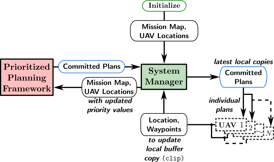
(a)

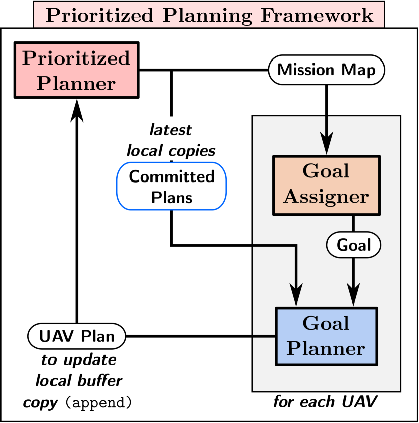
(b)

Figure 1: (1(a)) The System Manager (SM) communicates with all UAVs; it sends up-to-date copies of committed plans to corresponding UAVs and updates them using information received from the Prioritized Planner (PP) (1(b)) Prioritized planning framework: For each UAV, the Goal Assigner (GA) selects the next goal using the up-to-date map from the PP and the Goal Planner (GP) then plans a feasible path to this goal, which is appended to its committed plan

In this paper, we present a planning framework to address all the above questions. A block diagram of the complete framework is presented in Fig. 1. To the best of our knowledge, this work is the first to answer all of these questions in unison for real-world, persistent coverage with multiple robots. For our application, these robots are Unmanned Aerial Vehicles (UAVs). The System Manager (SM, Sec. 4.1) is our communication interface between the centralized planner and individual UAVs. It is responsible for back-and-forth communication of up-to-date information between the two. The Prioritized Planner (PP, Sec. 4.2) is responsible for answering Q3. Thereafter, the Goal Assigner (GA, Sec. 4.3) answers Q1 and specifies the location the next UAV should fly to. This is fed to the Goal Planner (GP, Sec. 4.4), which plans a kinodynamically feasible path for the UAV to the goal, answering Q2. Part of this plan is appended to the existing committed plan of the UAV. The PP, which operates continuously in a loop, then begins the next planning cycle, answering Q3 again.

We only append a part of computed plans to committed plans of UAVs (further detailed in Sec. 4). This is done so that we maintain committed plans of a pre-specified maximum duration (denoted by $t_{\text{max}}$). There is a trade-off involved in making $t_{\text{max}}$ too short or too long. Sec. 4 provides more insight into how and why this arises. We rely on globally deconflicting paths for UAVs since other, more local collision-checking mechanisms have a higher risk of causing deadlocks. Some other approaches utilise conflict detection and resolution systems to repair conflicting paths barnier2012trajectory . Our approach solves for deconflicting paths by construction and maintains the invariant of global deconfliction.

In Sec. 2, we contextualize our work among the Orienteering Problem (OP) vansteenwegen2011orienteering and the Vehicle Routing Problem (VRP) toth2002vehicle , coverage path-planning galceran2013survey , and frontier-based exploration yamauchi1998frontier . Sec. 3 formalizes the persistent-coverage problem we aim to solve and introduces the notion of priorities over coverage zones. Sec. 4 provides details about our planning framework and each of its constituent parts. In Sec. 5, we present results of the performance of our framework in both simulated and real-world environments. Finally, Sec. 6 discusses the consequences of some design-related decisions and proposed extensions.

2 Related Work

A majority of existing literature casts the persistent coverage problem as an instantiation of the OP or the VRP. An OP seeks to determine a path for an agent limited by a time- or distance-budget that visits a subset of all surveillance sites in an environment and maximizes the sum of associated scores collected. An extension of this to multiple agents is known as the Team Orienteering Problem (TOP) vansteenwegen2011orienteering . There are a number of works that apply solutions of the OP to surveillance with aerial vehicles over a small number of surveillance sites keller2016thesis . The formulation by Leahy et al. comes closest to our work because of its capability of assigning time windows to each coverage-zone as temporal logic constraints leahy2016persistent .

Given a number of agents at a depot and distances among all surveillance sites and the depot, the VRP seeks to find a minimum-distance tour for each agent such that it visits each site at least once. Michael et al. address persistent surveillance with aerial vehicles as a VRP with modifications to model continuous site visits golden2008vehicle ; stump2011multi .

The OP and VRP are both variants of the Traveling Salesman Problem (TSP) and thus NP-hard. Moreover, in our case, formulating the problem as a TOP or VRP is not enough since our problem also has an element of 2D coverage. One could consider every discrete part of the environment as a surveillance site in a TOP or VRP to enable 2D coverage, but this is impractical due to increasing computational complexity with the number of surveillance sites.

Smith et al. tackle a very similar problem by assuming pre-planned paths, decoupling path-planning and speed-control for deconfliction smith2011sweeping . Planning paths for 2D coverage has been extensively studied in robotics galceran2013survey . Typical solutions to static coverage involve environmental partitioning via Voroni tessellations and feedback control laws with local collision-avoidance schemes schwager2009decentralized . Environmental partitioning is also a recurring strategy for dynamic and persistent coverage MRC2kapoutsis2017darp . However, such partitioning restricts individual robots to specific parts of the environment.

For real-world settings, robot path-planners must adhere to kinodynamic motion-constraints. Thakur et al. solve the TOP and path-planning simultaneously to generate 3D ($x,y,\theta$) space-parametrized trajectories, but without temporal deconfliction thakur2013planning . Many also formulate planning for persistent surveillance as a mixed-integer linear program (MILP) bellingham2002coordination . However, such MILP formulations introduce limitations that are typically managed by planning for constant-speed paths ademoye2006trajectory .

A vital part of our framework is to ensure UAVs fly to appropriate goals, so that they simultaneously cover different parts of the environment. We adapt frontier-based exploration to assign such goals to UAVs. Yamauchi et al. first proposed this for single and multiple robots based on an occupancy-grid representation of the environment yamauchi1998frontier . Many extensions have been proposed since then, which combine the information gain or expected benefit of the goal and the distance to it, also called next-best-view approaches adler2014autonomous . Zhu et al. also apply this to exploration and coverage with micro aerial vehicles (MAVs) zhu2015mavs . We use frontier-based exploration to trade off between cell-proximity and cell-criticality (defined formally in Sec. 3). To be able to do this online, we use a search-based approach similar to Butzke et al. butzke2011planning .

3 Problem Formulation

Our problem definition is characterized by a mission-map $\mathcal{M}$, and a set of $N$ UAVs $\{U_{1},\ldots,U_{N}\}$, tasked with covering the area represented by $\mathcal{M}$. Each UAV $U_{k}$ is a kinodynamically constrained system, with an associated coverage- or sensor-radius $r_{k}$. Let the cell at row $i$ and column $j$ of $\mathcal{M}$ be $c_{i,j}$. A UAV $U_{k}$ is at cell $c_{i,j}$ if the projection of its reference point onto the $x,y$ plane (denoted by $U_{k}^{\text{loc}}$) lies in cell $c_{i,j}$. A cell is said to be covered by a UAV flying over it if any point on the cell is at at most an $r_{k}$ distance from $U_{k}^{\text{loc}}$. This effectively assumes a circular sensor-footprint of radius $r_{k}$ centered around $U_{k}^{\text{loc}}$. Each cell $c_{i,j}$ is associated with two temporal properties—its lifetime $\ell(c_{i,j})$ and its age $a(c_{i,j})$. The age of a cell is the time passed since the cell was last covered by a UAV, while its lifetime is a desired bound on its age (as shown in Fig. 2).

There are two types of cells in our problem specification: (i) standard cells (that UAVs need to cover), and (ii) obstacle cells (that UAVs cannot fly over). Based on this, we define the following maps:

1. Priority Map, $\mathcal{M}^{\text{P}}=\left\{c_{i,j}:c_{i,j}\text{ is a standard cell}\wedge\ell(c_{i,j})<\infty\right\}$. In other words, $\mathcal{M}^{\text{P}}$ is the set of all standard cells that a UAV will need to cover in finite time since the start of the mission.

2. No-coverage Map, $\mathcal{M}^{\text{NC}}=\left\{c_{i,j}:c_{i,j}\text{ is a standard cell}\wedge\ell(c_{i,j})=\infty\right\}$. In other words, $\mathcal{M}^{\text{NC}}$ is the set of all standard cells in the mission-map that a UAV can fly over, but does not need to cover.

3. Obstacle Map, $\mathcal{M}^{\text{O}}=\left\{c_{i,j}:c_{i,j}\text{ is an obstacle cell}\right\}$.

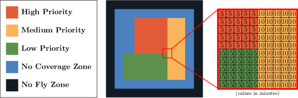
Figure 2: An example of a mission-map $\mathcal{M}$, where each cell is colored according to its lifetime. For example, a green cell with a lifetime of $15$ minutes implies that no more than 15 minutes should pass between two consecutive times a UAV covers it.

The mission-map can then be defined as $\mathcal{M}=\mathcal{M}^{\text{P}}\cup\mathcal{M}^{\text{NC}}\cup\mathcal{M}^{\text{O}}$. Fig. 2 contains an example of a mission-map with three different priority-levels. Given a mission-map and a set of UAVs, our problem is to compute UAV-plans such that the following properties hold:

1. Feasibility—the motion of each UAV adheres to its kinodynamic constraints.

2. Deconfliction—no two UAVs collide. In our specific setting, all UAVs are constrained to fly at the same altitude, so we say that two UAVs $U_{p}$ and $U_{q}$ collide if they come within some predefined distance $d_{\text{min}}$ of each other.

3. Persistence—the age of each cell is smaller or equal to its lifetime.

4. Flexibility—UAVs can be dynamically added or removed to the system.

P1 and P2 are hard constraints that must always be satisfied. P3 depends on the mission specification—the number of UAVs deployed, their capabilities (speed, sensor radii etc.) and the mission-map (size and lifetime of each cell). Our framework supports P4 without affecting P1 and P2, however it will affect (help or hinder) our ability to satisfy P3.

4 Approach

Our approach, depicted in Fig. 1, consists of a System Manager (SM) which serves as an interface between the centralized planning framework and individual UAVs. It maintains the priority map $\mathcal{M}^{\text{P}}$ by updating locations of individual UAVs. Every planning cycle, the SM passes the three maps to the Prioritized Planner (PP). The PP then iterates over all the UAVs in a round-robin fashion. For each UAV $U_{k}$, it generates a local copy of $\mathcal{M}^{\text{P}}_{k}$ that accounts for the committed plans of the other UAVs. This priority map $\mathcal{M}^{\text{P}}_{k}$ is used by the Goal Assigner (GA) to assign a goal (in terms of $x,y$ location) for the UAV $U_{k}$. A kinodynamically feasible path to reach this goal is then computed for $U_{k}$ using the Goal Planner (GP).

A key notion used within our framework is that of committed plans, which are collision-free plans each UAV is committed to execute. While the GP might compute plans of long durations (if the goal is far away or plan execution requires long, feasible maneuvers), only a portion of this plan will be added to the committed plan, such that it is at most $t_{\text{max}}$ long in time. The value of $t_{\text{max}}$ must be decided based on the mission since the following effects introduce a trade-off:

1. Effects of a high value for $t_{\text{max}}$:

   • The longer the committed plans are, the less reactive UAVs are to any map updates including updates by an operator.

   • The path computed by the GP might take $U_{k}$ through areas coinciding with parts of the committed plans of $U_{j\neq k}$ before $U_{j\neq k}$ covers them. This results in redundant coverage. The chances of this happening increase as $t_{\text{max}}$ increases.

2. Effects of a low value for $t_{\text{max}}$:

   • The shorter the committed plan, the lesser the chance of deviating from it during execution due to imperfect controllers. However, this increases the chances of UAV $U_{k}$ executing the committed plan before the next planning cycle ends, leaving the UAV’s controller with no plan to execute. We handle this by ensuring that the UAV can execute a stopping-maneuver in this situation, but repeated execution of stopping-maneuvers is undesirable.

   • Having short committed plans increases the frequency of goal assignment for a UAV. This causes two adverse effects: (i) A UAV may be assigned a new goal that is different from its previous one, which would cause it to abandon trying to reach the previous goal. (ii) Even if the same goal is assigned, it might lead to “plan thrashing”. A UAV’s complex dynamics may restrict short plans from letting it make significant progress towards a goal if complicated maneuvers are required.

4.1 System Manager

The System Manager (SM) is the communication interface between the centralized planner and the individual UAVs, shown in Fig. 1 (left): The SM sends the mission-map $\mathcal{M}$ to the PP, and it receives the updated committed plans from the PP and sends them out to the respective UAVs. It maintains the priority map $\mathcal{M}^{\text{P}}$ by: (i) resetting the age of any standard cells that have been covered since the last update to zero, and (ii) incrementing the age of all other standard cells.

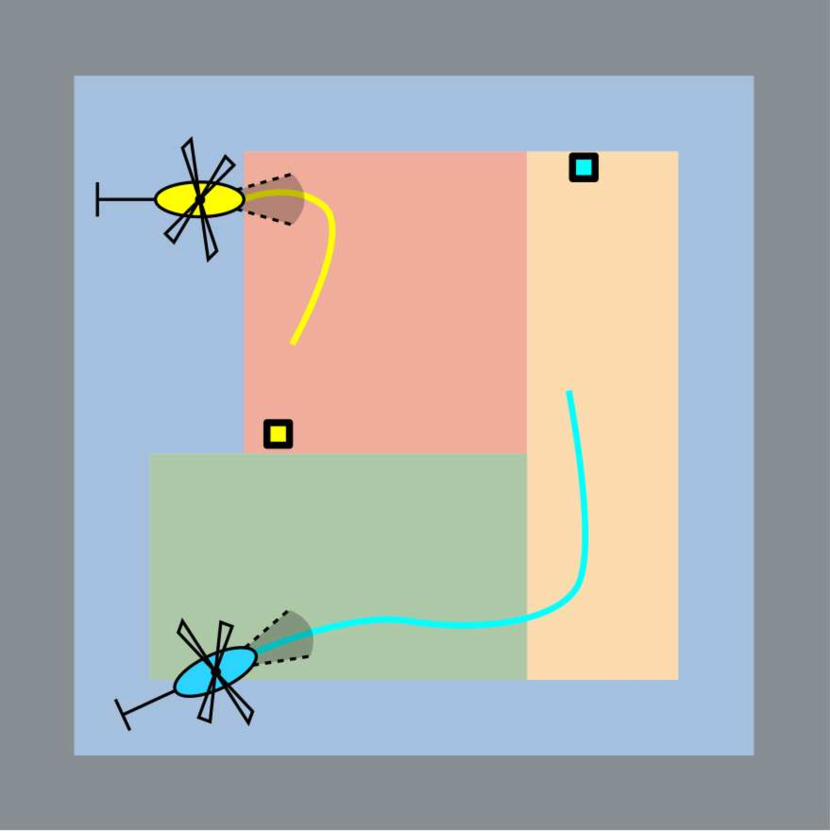
(a)

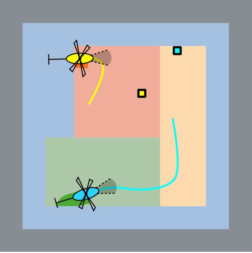
(b)

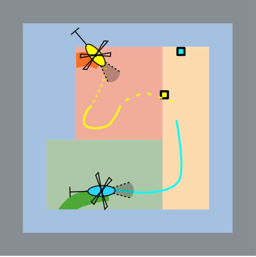
(c)

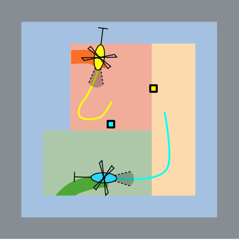
(d)

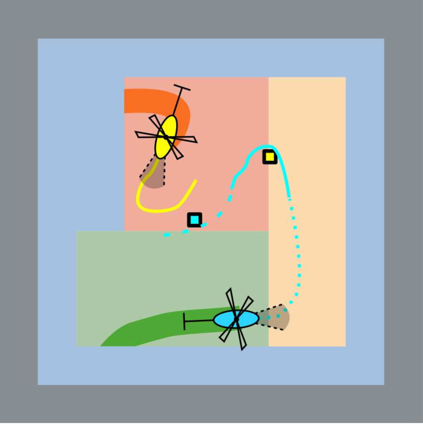
(e)

Figure 3: Two successive executions of the GA-GP loop (the map $\mathcal{M}$ is colored with 50% opacity). (3(a)) The solid yellow and blue lines show committed plans for both UAVs. (3(b)) A new goal is assigned to the yellow UAV. (3(c)) A path planned is for the yellow UAV (the old committed plan is a dotted line, the new committed plan is a solid line, and the discarded part of the new plan is a dashed line). (3(d)) The same as (3(b)) but for the blue UAV. (3(e)) The same as (3(b)) but for the blue UAV.

4.2 Prioritized Planner

The Prioritized Planner (PP) is a state-machine that controls our centralized planning framework by continuously executing RunPlanner from Alg. 1. During each execution of RunPlanner, which we call a planning cycle, the PP is responsible for the following tasks:

1. Update its local copy of the committed plans and $\mathcal{M}^{\text{P}}$ to reflect the most recent information received from the SM.

2. Determine which UAV will be planned for during this cycle.

3. Perform a new goal assginment for the UAV and plan a path to it.

4. Communicate the result of T3 throughout the framework.

T1 is performed in Lines 4–6 in Alg. 1. The PP clips the part of its local copy of committed plans that have been executed by the UAVs since the last planning cycle, and accounts for the part yet to be executed by resetting the age of all the cells in $\mathcal{M}^{\text{P}}$ that will be covered by the committed plans to zero.

We do not prioritize any one UAV over the others, which corresponds to the PP selecting UAVs in a round-robin fashion, thus achieving T2. While the PP supports a prioritization over UAVs, in our experience, assigning equal priorities in this way showed satisfactory performance.

T3 is achieved through one iteration of the GA-GP loop shown in Fig. 1(b). For ease of understanding, we show two successive executions of this loop in Fig. 3. Fig. 3(b) and 3(c) correspond to Lines 9 and 10 for the yellow UAV. Fig. 3(d) and 3(e) correspond to the same lines for the blue UAV.

T4 is performed by Lines 11–13. First, we append to a UAV’s committed plan to bring it up to $t_{\text{max}}$ in length. Second, $\mathcal{M}^{\text{P}}$ is updated to account for this new plan (same as in Line 6) by resetting the age of all the cells that will be covered. Finally, the newly committed plan is communicated to the UAV via the SM.

Algorithm 1 Prioritized Planner Loop

1:procedure RunPlanner

2:    $N\leftarrow$ number of UAVs

3:    while true do

4:         Get latest $\mathcal{M}=\left\{\mathcal{M}^{\text{P}},\mathcal{M}^{\text{NC}},\mathcal{M}^{\text{O}}\right\}$ and $U_{1:N}^{\text{loc}}$ from SM

5:         Update committed plans (local copies) by using $U_{1:N}^{\text{loc}}$ $\triangleright$ Clip

6:         Update $\mathcal{M}^{\text{P}}$ with committed plans

7:         for $k\leftarrow 1:N$ do

8:             if committed plan for $U_{k}$ is short then

9:                 $G_{k}\leftarrow\textsc{GetGoal}\left(\mathcal{M}^{\text{P}}\right)$ $\triangleright$ Goal assignment (GA)

10:                 $\pi_{k}\leftarrow\textsc{GetPlan}\left(\mathcal{M},G_{k}\right)$ $\triangleright$ Goal planning (GP)

11:                 Update committed plan for $U_{k}$ with $\pi_{k}$ $\triangleright$ Append a portion of $\pi_{k}$

12:                 Update $\mathcal{M}^{\text{P}}$ with committed plan for $U_{k}$

13:                 Send committed plan for $U_{k}$ to SM                           

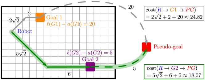
Figure 4: Multi-goal Dijkstra search for goal assignment finds the least-cost path to a pseudo-goal connected to all potential goal locations for a robot. It considers the cost of reaching a potential goal from the robot’s location, and the priority of a goal location reflected in the cost of the edge connecting it to the pseudogoal. In the example above, goal G2 is assigned to the robot.

4.3 Goal Assigner

Recall that the Goal Assigner (GA) selects a goal for each UAV to fly to. The grid $\mathcal{M}^{\text{P}}_{k}$ is the local copy of the Priority Map ($\mathcal{M}^{\text{P}}$) that belongs to UAV $U_{k}$. Each of the cells in the eight-connected grid that represents $\mathcal{M}^{\text{P}}_{k}$ is a potential goal for $U_{k}$. The GA computes a goal-location $G_{\text{k}}$ for each UAV, accounting for how urgent every cell in $\mathcal{M}^{\text{P}}_{k}$ is and the location of the UAV $U_{k}$. To simultaneously reason about the urgency of the goal and its distance from $U_{k}$, we build a graph by connecting a pseudo-goal to every cell of the grid $\mathcal{M}^{\text{P}}_{k}$. The pseudo-goal is an “imaginary” state connected by “imaginary” pseudo-edges to all cells in the grid as shown in Fig. 4. The cost of these pseudo-edges is proportional to $(\ell(i,j)-a(i,j))$. The costs of the rest of the edges between adjacent cells in the grid are equal to the Euclidean distance between them.

To find an optimal goal $G_{k}$, we first find an optimal path from $U_{k}^{\text{loc}}$ to the pseudo-goal on this graph using Dijkstra’s search dijkstra1959note . The optimal path minimizes the sum of the costs of the real-edges (which reflects the cost to reach the goal) and the cost of the pseudo-edge (which reflects the priority of the cell that the pseudo-edge connects). The final goal $G_{k}$ for UAV $U_{k}$ is the parent of the pseudo-goal on this optimal path.

4.4 Goal Planner

Once a goal is assigned to $U_{k}$, the GP computes a kinodynamically feasible path to it via search-based planning on a state-lattice likhachev2009planning ; pivtoraiko2005generating . The state-space for each UAV includes its two-dimensional pose $(x,y,\theta)$, linear velocity $v$, and time $t$. Assuming double-integrator dynamics for each UAV, we generate an action-space consisting of feasible motion primitives. These primitives use cells of size $1$\mathrm{m}$\times 1$\mathrm{m}$$. This discretization is independent of the mission-map discretization. We implicitly construct a graph using the action space during a weighted-A* search to the goal hart1968formal ; pohl1970heuristic . The search prunes away all transitions that correspond to trajectories that either intersect no-fly zones or collide with the committed plans of other vehicles in space or time. We terminate the search as soon as a state is expanded whose incoming edge (from the predecessor on the found path) covers the goal cell (specifically, the trajectory corresponding to this edge contains a point whose distance to the goal cell is less than $r_{k}$). We assign the time taken to execute an action as its edge-cost in the graph. While our aim is to plan for minimum-time paths, it is also desirable for the UAVs to fly at high speeds whenever possible and avoid stopping. For this reason, we incentivize actions with increasing velocities, penalize actions with decreasing velocities, and heavily penalize hovering.

5 Experimental Setup and Results

We evaluate our framework in both simulation, where we assume perfect state estimation and control, and on real UAVs, which can deviate from their planned paths. The UAVs can withstand winds of speeds up to $30\text{\,}\mathrm{m}\text{/}\mathrm{s}$. Thus, the effect of wind is negligible under normal conditions. Accounting for large deviations from planned paths requires replanning and is part of future work. Our framework uses an identical set of parameters in both cases. We generate motion primitives with a maximum speed of $6\text{\,}\mathrm{m}\text{/}\mathrm{s}$ and a maximum turning rate of $6\text{\,}\mathrm{\SIUnitSymbolDegree}\text{/}\mathrm{s}$. We avoid adding angular velocity to the state-space by ensuring that these primitives start and end at zero angular velocity. Two UAVs are deemed to have collided if at any point in time the distance between these 2D locations is less than $d_{\text{min}}=10\ $\mathrm{m}$$. The parameter $r_{\text{k}}=15\ $\mathrm{m}$$ defines the circular area directly underneath a UAV that is deemed covered for any 2D location of the UAV. We impose a planning timeout of $4\ $\mathrm{s}$$ on the Goal Planner, which is how long it is given to compute a plan. We use an Euclidean-distance heuristic in the Weighted-A* search pohl1970heuristic with an inflation of $5$. Fig. 7(d) and 7(e) shows the two coverage-maps used for the experiments presented in this paper.

5.1 Evaluation Metrics

We look at timing statistics for Goal Assignment ($t_{\text{GA}}$) and Goal Planning ($t_{\text{GP}}$), number of state expansions, and number of expansions per second. Since we desire continued movement from each UAV, we also look at the amount of time a UAV is stationary on average across the simulation run ($t_{\text{stopped}}$). Additionally, we evaluate our framework’s performance with respect to the criticality of a cell, defined for any cell $(i,j)$ at timestamp $t$ as $C_{t}(i,j)=\frac{a_{t}(i,j)}{\ell(i,j)}$ , where $C_{t}:\mathbb{E}(2)\rightarrow\mathbb{R}$ is a time-varying measure of criticality. $C_{t}(i,j)$ starts with a value of zero and as the cell ages over time, $C_{t}(i,j)$ starts to increase. Once the age of a cell reaches its lifetime—namely, $C_{t}(i,j)$ equals one—we say that the cell has expired. If we average this value across all cells in the map to be covered, we obtain an estimate idea of how well a team of UAVs is covering the areas they have been assigned:

$$\bar{C}_{t}=\frac{1}{|\mathcal{M}^{\text{P}}|}\sum_{(i,j)\in\mathcal{M}^{\text{P}}}C_{t}(i,j)\vspace{-9pt}$$ (1)

Given this measure of criticality, ideal behavior would be to keep the value of $\bar{C}_{t}$ constant over the course of a mission, a lower value being better.

5.2 Simulation Experiments

Hardware Platform Simulation experiments were performed on a desktop computer running Ubuntu 16.04 and equipped with an Intel Core i7-4790K processor and 20 GB of RAM.

Planner Evaluation We present simulation results on both maps from Fig. 7 for $10$ minutes in Table 5.2. We observe that by increasing the number of UAVs, Goal Assignment times are not affected, whereas Goal Planning times increase significantly since GP must now compute deconflicting plans for a larger number of UAVs. Despite this, the total amount of stationary time spent by a UAV was at most $19.90\ $\mathrm{s}$$ in a $10$-minute period. Fig. 5 shows a plot of $\bar{C}_{t}$ (Eq. (1)) over time during a 30-minute mission. In all experiments, our framework is able to keep $\bar{C}_{t}$ below a value of one except where the number of UAVs was too small given the size of the map (experiment with one UAV and map from Fig. 7). This, along with the fact that all plots plateau over time, implies that cell-expiration is regulated on average.

Map		Number of UAVs		Timing (ms)				Path Planning
				$t_{GA}$
	$t_{GP}$
	$t_{Total}$
		Number of
	Expansions	Expansions
	$t_{\text{stopped}}$
	(%)
Fig. 7(d)		1		90	223	323		413	215	0
		2		90	796	898		187	226	2
		3		91	1326	1430		286	209	2
Fig. 7(e)		1		92	172	275		28	204	0
		2		91	1163	1265		200	188	< 1
		3		91	1433	1536		248	185	3

Table 1: Results of simulation experiments (values rounded down to the closest integer) and $t_{\text{stopped}}$ expressed as a percentage of total mission time.

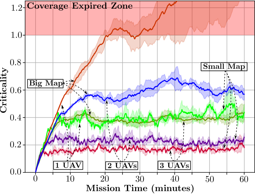
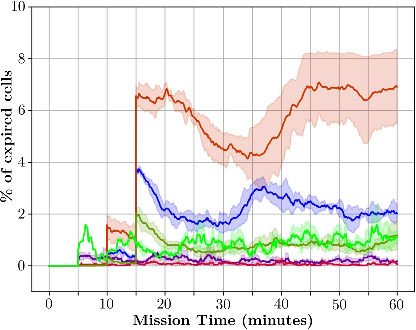
Figure 5: Left: Average criticality of cells in $\mathcal{M}^{\text{P}}$ during simulated experiments. Right: Spikes occur at 5, 10, 15 minutes since these are the three different cell lifetimes in the initial $\mathcal{M}^{\text{P}}$. Colors are consistent across the two plots.

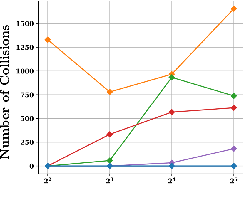
(a)

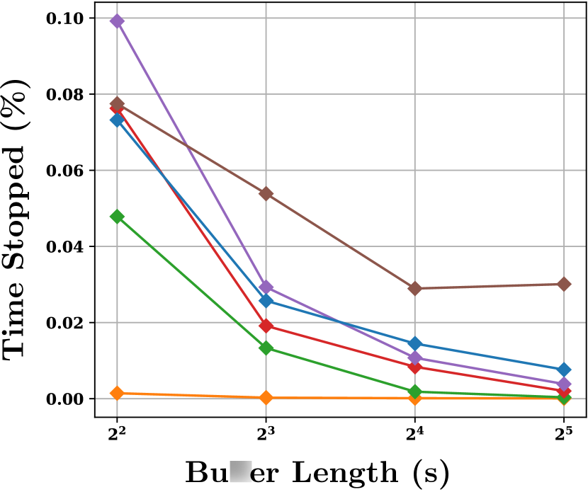
(b)

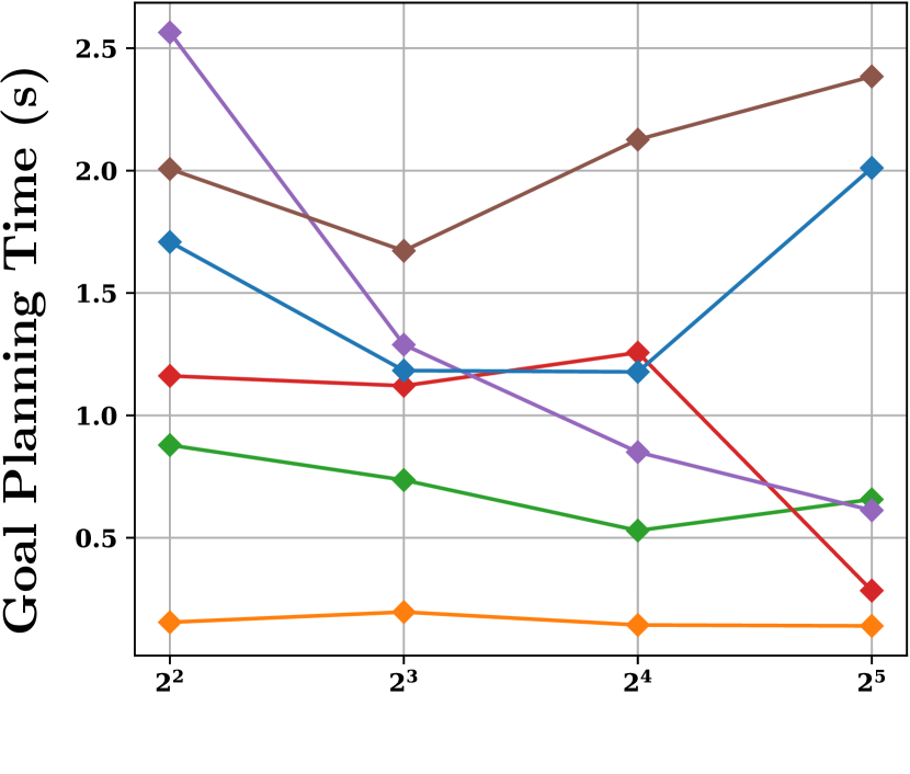
(c)

Figure 6: Effect of changing the committed plan length for different collision checking mechanisms. Since each curve represents a single mission execution, we do not show confidence intervals. The lines for Full Plan (static) and Our Framework coincide in (a).

Global Deconfliction Satisfactory global deconfliction relies on each UAV always having access to committed plans that are long enough. As discussed in Sec. 4, size of committed plans can significantly affect performance. We empirically evaluate the need and effect of global deconfliction by varying the lengths of committed plans for different collision-checking schemes. These schemes are:

1. Proposed Framework: Our approach with global deconfliction.

2. No Collision Checking: The GP performs no collision-checking between UAVs.

3. Current Position (static): The GP considers the other UAVs’ current positions as static obstacles.

4. Quarter, Half and Full Plan (static): The GP assumes the first quarter, half and whole of the committed plans of other UAVs to be static obstacles respectively.

We plot the number of collisions between UAVs in Fig. 6(a), the average time a UAV is stationary in Fig. 6(b), and the time taken by the Goal Planner in Fig. 6(c), all against varying lengths of committed plans. Fig. 6 shows that our deconfliction scheme results in competitive planning times and also guarantees collision-free UAV movement with negligible stoppage. Other collision-checking schemes are either overly conservative and compute convoluted, long-winding paths, or simply fail to avoid collisions.

5.3 Real-World Experiments

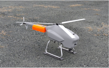
(a)

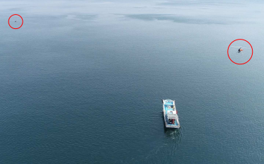
(b)

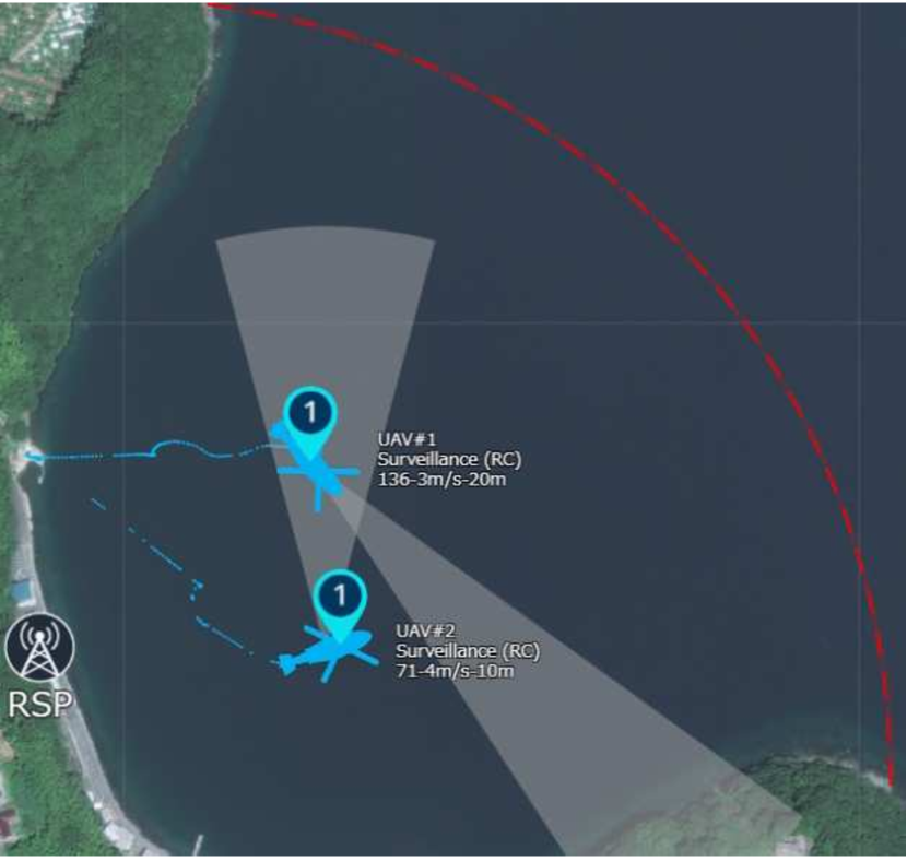
(c)

(d)

(e)

Figure 7: (7(a)) UAV used in the experiments. (7(b)) The two UAVs (circled in red) executing a mission. (7(c)) GUI showing a satellite image of the mission site along with UAV data overlay. (7(d)) Map used for experiments (big; coverage zone roughly $400\text{m}\times 400\text{m}$). (7(e)) Map used for experiments (small; coverage zone roughly $200\text{m}\times 100\text{m}$)

Hardware Setup For the real-world experiments, our planning framework was run on a Lenovo T470s laptop running Ubuntu 16.04 and equipped with an Intel Core i7-7600U processor and 20 GB of RAM.

Planner Evaluation We present results from real-world experiments in Table 5.3. Fig. 8(a) plots $\bar{C}_{t}$ for eight real-world runs. Additionally, dynamic removal of UAVs from the mission was tested in five of these runs, and the remaining UAVs were left undisturbed. Beyond this point, we are only covering the area with one UAV. Hence, it is expected to see criticality increase. By iteratively planning and executing computed paths, we isolate our planner from the stochasticity of controller-based execution in the real world. Our planner quantitatively performs just as well in the real-world as it does in simulation in spite of this stochasticity. This is because our framework seeks latest information about UAV and map statuses from the real world and constantly uses it to repeatedly solve our myopic version of the full problem (as explained in Sec. 4).

Map		Number of UAVs		Timing (ms)				Path Planning
				$t_{\text{GA}}$	$t_{\text{GP}}$	$t_{\text{total}}$		Number of
	Expansions							Expansions
	$t_{\text{stopped}}$
	(%)
Fig. 7(e)		1		105	240	363		37	186	0.00
		2		117	1181	1325		162	152	7.12

Table 2: Results of real-world experiments averaged over 8 runs (rounded down to the nearest integer) and $t_{\text{stopped}}$ expressed as a percentage of total mission time (maximum over all runs).

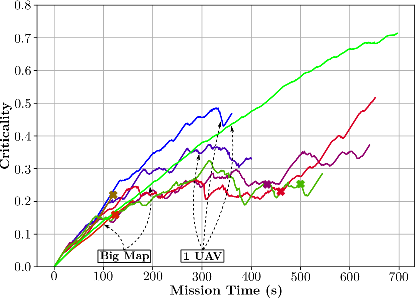
(a)

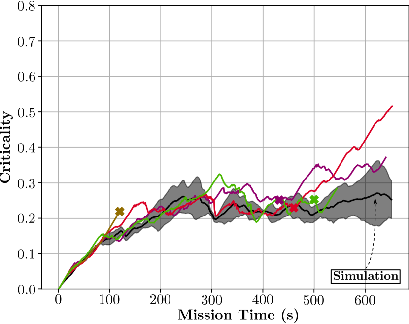
(b)

Figure 8: (a) Coverage criticality over time in the real-world: unless explicitly pointed to by arrows, the curves represent an experiment with two UAVs run on the smaller map. A cross ($\times$) on a curve indicates the point in time when one of the two UAVs was removed from the mission. (b) Comparison of all simulation and real-world missions executed in the small map from Fig. 7(e) by two UAVs. The black curve with confidence intervals corresponds to the simulated experiments.

6 Conclusion and Future Work

We present and evaluate a planning framework for real-world, persistent coverage with multiple UAVs. Our framework continuously decides where UAVs should fly and computes kinodynamically feasible, globally deconflicting plans. We evaluate our framework in both simulated and real-world settings. We also motivate and compare global deconfliction with weaker, more local collision-avoidance schemes.

In many practical settings like ours, state spaces are high-dimensional and time for deliberation is limited. Planning times can be a bottleneck in these cases and cause delays. While our stopping maneuvers handle such situations, a natural extension is to incorporate anytime planning sun2008generalized .

In the current framework, the goal assignment is based on priorities and is decoupled from goal planning. This is greedy and not optimal. Better strategies to repeatedly cover previously observed coverage-zones can be learned from data and added as macro-actions in the planner.

References

- (1) Ademoye, T.A., Davari, A.: Trajectory planning for multiple autonomous systems using mixed integer linear programming. In: Proceedings of the Thirty-Eighth Southeastern Symposium on System Theory, pp. 175–179. IEEE (2006)
- (2) Adler, B., Xiao, J., Zhang, J.: Autonomous exploration of urban environments using unmanned aerial vehicles. Journal of Field Robotics 31(6), 912–939 (2014)
- (3) Arkin, E.M., Hassin, R.: Approximation algorithms for the geometric covering salesman problem. Discrete Applied Mathematics 55(3), 197–218 (1994)
- (4) Barnier, N., Allignol, C.: Trajectory deconfliction with constraint programming. The Knowledge Engineering Review 27(3), 291–307 (2012)
- (5) Bellingham, J.S.: Coordination and control of UAV fleets using mixed-integer linear programming. Ph.D. thesis, Massachusetts Institute of Technology (2002)
- (6) Butzke, J., Likhachev, M.: Planning for multi-robot exploration with multiple objective utility functions. In: IROS, pp. 3254–3259 (2011)
- (7) Dijkstra, E.W.: A note on two problems in connexion with graphs. Numerische mathematik 1(1), 269–271 (1959)
- (8) Erdmann, M., Lozano-Perez, T.: On multiple moving objects. Algorithmica 2(1-4), 477 (1987)
- (9) Franco, C., López-Nicolás, G., Sagüés, C., Llorente, S.: Persistent coverage control with variable coverage action in multi-robot environment. In: CDC, pp. 6055–6060 (2013)
- (10) Galceran, E., Carreras, M.: A survey on coverage path planning for robotics. Robotics and Autonomous Systems 61(12), 1258–1276 (2013)
- (11) Golden, B.L., Raghavan, S., Wasil, E.A.: The vehicle routing problem: latest advances and new challenges, vol. 43. Springer Science & Business Media (2008)
- (12) Hart, P.E., Nilsson, N.J., Raphael, B.: A formal basis for the heuristic determination of minimum cost paths. IEEE Transactions on Systems Science and Cybernetics 4(2), 100–107 (1968)
- (13) Kapoutsis, A.C., Chatzichristofis, S.A., Kosmatopoulos, E.B.: DARP: divide areas algorithm for optimal multi-robot coverage path planning. Journal of Intelligent & Robotic Systems 86(3-4), 663–680 (2017)
- (14) Keller, J.F.: Path planning for persistent surveillance applications using fixed-wing unmanned aerial vehicles. Computers & Operations Research (2016)
- (15) Leahy, K., Zhou, D., Vasile, C.I., Oikonomopoulos, K., Schwager, M., Belta, C.: Persistent surveillance for unmanned aerial vehicles subject to charging and temporal logic constraints. Auton. Robots 40(8), 1363–1378 (2016)
- (16) Likhachev, M., Ferguson, D.: Planning long dynamically feasible maneuvers for autonomous vehicles. IJRR 28(8), 933–945 (2009)
- (17) Mellone, A., Franzini, G., Pollini, L., Innocenti, M.: Persistent coverage control for teams of heterogeneous agents. In: CDC, pp. 2114–2119 (2018)
- (18) Nedjati, A., Izbirak, G., Vizvari, B., Arkat, J.: Complete coverage path planning for a multi-UAV response system in post-earthquake assessment. Robotics 5(4), 26 (2016)
- (19) Pivtoraiko, M., Kelly, A.: Generating near minimal spanning control sets for constrained motion planning in discrete state spaces. In: IROS, pp. 3231–3237 (2005)
- (20) Pohl, I.: Heuristic search viewed as path finding in a graph. Artificial intelligence 1(3-4), 193–204 (1970)
- (21) Schwager, M., Rus, D., Slotine, J.J.: Decentralized, adaptive coverage control for networked robots. IJRR 28(3), 357–375 (2009)
- (22) Smith, R.N., Schwager, M., Smith, S.L., Jones, B.H., Rus, D., Sukhatme, G.S.: Persistent ocean monitoring with underwater gliders: Adapting sampling resolution. JFR 28(5), 714–741 (2011)
- (23) Smith, S.L., Schwager, M., Rus, D.: Persistent robotic tasks: Monitoring and sweeping in changing environments. arXiv preprint arXiv:1102.0603 (2011)
- (24) Srinivasan, S., Latchman, H., Shea, J., Wong, T., McNair, J.: Airborne traffic surveillance systems: video surveillance of highway traffic. In: Proceedings of the ACM 2nd international workshop on Video surveillance & sensor networks, pp. 131–135 (2004)
- (25) Stump, E., Michael, N.: Multi-robot persistent surveillance planning as a vehicle routing problem. In: IEEE International Conference on Automation Science and Engineering, pp. 569–575 (2011)
- (26) Sun, X., Koenig, S., Yeoh, W.: Generalized adaptive A*. In: AAMAS, pp. 469–476. International Foundation for Autonomous Agents and Multiagent Systems (2008)
- (27) Teixeira, L., Alzugaray, I., Chli, M.: Autonomous aerial inspection using visual-inertial robust localization and mapping. In: FSR, pp. 191–204. Springer (2018)
- (28) Thakur, D., Likhachev, M., Keller, J., Kumar, V., Dobrokhodov, V., Jones, K., Wurz, J., Kaminer, I.: Planning for opportunistic surveillance with multiple robots. In: IROS, pp. 5750–5757 (2013)
- (29) Toth, P., Vigo, D.: The vehicle routing problem. SIAM (2002)
- (30) Vansteenwegen, P., Souffriau, W., Van Oudheusden, D.: The orienteering problem: A survey. European Journal of Operational Research 209(1), 1–10 (2011)
- (31) Yamauchi, B., et al.: Frontier-based exploration using multiple robots. In: Agents, vol. 98, pp. 47–53 (1998)
- (32) Zhu, C., Ding, R., Lin, M., Wu, Y.: A 3D frontier-based exploration tool for MAVs. In: ICTAI, pp. 348–352 (2015)