Circle Graph Isomorphism in Almost Linear Time

Abstract

Circle graphs are intersection graphs of chords of a circle. In this paper, we present a new algorithm for the circle graph isomorphism problem running in time ${\mathcal{O}}((n+m)\alpha(n+m))$ where $n$ is the number of vertices, $m$ is the number of edges and $\alpha$ is the inverse Ackermann function. Our algorithm is based on the minimal split decomposition [Cunnigham, 1982] and uses the state-of-art circle graph recognition algorithm [Gioan, Paul, Tedder, Corneil, 2014] in the same running time. It improves the running time ${\mathcal{O}}(nm)$ of the previous algorithm [Hsu, 1995] based on a similar approach.

1 Introduction

For graphs $G$ and $H$, a bijection $\pi:V(G)\to V(H)$ is called an isomorphism if $uv\in E(G)\iff\pi(u)\pi(v)\in E(H)$. Testing isomorphism of graphs in polynomial time is a major open problem in theoretical computer science. The graph isomorphism problem clearly belongs to NP, it is unlikely NP-complete [40], and the best known algorithm runs in quasipolynomial time [2], heavily based on group theory. For a survey, see [27].

For restricted classes of graphs, it is often possible to design combinatorial polynomial-time algorithms, relying on strong structural properties of the considered classes: prime examples are linear-time algorithms for testing isomorphism of trees [1] and planar graphs [23, 18, 25]. Testing isomorphism of interval graphs [36] and permutation graphs [9, 31] in linear time relies on the property that certain canonical trees describe all their representations, and thus it can be reduced to testing isomorphism of trees whose nodes are labeled by simple graphs. In this paper, we described an almost linear-time algorithm for testing isomorphism of circle graphs working in a similar spirit.

For a graph $G$, a circle representation ${\mathcal{R}}$ of a graph $G$ is a collection of sets $\bigl{\{}\left<v\right>:v\in V(G)\bigr{\}}$ such that each $\left<v\right>$ is a chord of some fixed circle, and $\left<u\right>\cap\left<v\right>\neq\emptyset$ if and only if $uv\in E(G)$. Observe that ${\mathcal{R}}$ is determined by the circular word giving the clockwise order of endpoints of the chords in which $uv\in E(G)$ if and only if their endpoints alternate as $uvuv$ in this word. A graph is called a circle graph if and only if it has a circle representation; see Fig. 1.

Figure 1: A circle graph and one of its circle representations corresponding to the circular word $10,2,1,7,8,10,9,5,6,8,7,3,4,6,5,1,2,4,3,9$.

Circle graphs were introduced by Even and Itai [17] in the early 1970s. They are related to Gauss words [15], matroid representations [6, 14], and rank-width [39]. The complexity of recognition of circle graphs was a long-standing open problem, resolved in mid-1980s [5, 19, 37]. Currently, the fastest recognition algorithm [20] runs in almost linear time. In this paper, we use this recognition algorithm as a subroutine and solve the graph isomorphism problem of circle graphs in the same running time.

Theorem 1.1.

The graph isomorphism problem of circle graphs and the canonization problem of circle graphs can be solved in time ${\mathcal{O}}((n+m)\cdot\alpha(n+m))$, where $n$ is the number of vertices, $m$ is the number of edges, and $\alpha$ is the inverse Ackermann function. Further, if circle representations are given as a part of the input, the running time improves to ${\mathcal{O}}(n+m)$.

Two circle representation are isomorphic if by relabeling the endpoints we get identical circular orderings. In Section 4, we show that isomorphism of circle representations can be tested in time ${\mathcal{O}}(n)$. When circle graphs $G$ and $H$ have isomorphic circle representations ${\mathcal{R}}_{G}$ and ${\mathcal{R}}_{H}$, clearly $G\cong H$. But in general, the converse does not hold since a circle graph may have many non-isomorphic circle representations.

The main tool is the split decomposition which is a recursive process decomposing a graph into several indecomposable graphs called prime graphs. Each split decomposition can be described by a split tree whose nodes are the prime graphs on which the decomposition terminates. The key property is that the initial graph is a circle graph if and only if all prime graphs are circle graphs. Further, each prime circle graph has a unique representation up to reversal, so isomorphism for them can be tested in ${\mathcal{O}}(n)$ using Section 4.

One might want to reduce the isomorphism problem of circle graphs to the isomorphism problem of split trees. Unfortunately, a graph may posses many different split decompositions corresponding to non-isomorphic split trees. The seminal paper of Cunnigham [10, Theorem 3] shows that for every connected graph, there exists a minimal split decomposition; this result was also proven in [11, Theorem 11]. The split tree associated to the minimal split decomposition is then also unique and it follows that the isomorphism problem of circle graphs reduces to the isomorphism problem of minimal split trees.

Already in 1995, this approach was used by Hsu [24] to solve the graph isomorphism problem of circle graphs in time ${\mathcal{O}}(nm)$. He actually concentrates on circular-arc graphs, which are intersection graphs of circular arcs, and builds a decomposition technique which generalizes minimal split decomposition. The main results are recognition and graph isomorphism algorithms for circular-arc graphs running in ${\mathcal{O}}(nm)$. Unfortunately, a mistake in this general decomposition technique was pointed out by [12].

This discovered mistake does not affect the graph isomorphism algorithm for circle graphs. However, Hsu’s 29 page long paper [24] just briefly mentions circle graphs and minimal split decomposition, with many details omitted. Also, a straightforward adaptation of Hsu’s algorithm combined with the fastest algorithm computing the minimal split decomposition implies an ${\mathcal{O}}(n^{2})$ algorithm for testing isomorphism of circle graphs. But to get almost linear running time, further problems have to be addressed in this paper.

In [35], a linear-time algorithm testing isomorphism of proper circular-arc graphs is described. These are intersection graphs of circular arcs such that no arc is properly contained in another one. Since proper circular-arc graphs form a subclass of circle graphs, we strengthen their result.

Outline.

Section 2 gives an overview of minimal split decomposition and minimal split trees. In Section 3, we describe a meta-algorithm computing cannonical form of a general tree whose nodes are labeled by graphs for which a linear-time cannonization is known. For a circle graph, its unique minimal split tree is labeled by prime circle graphs and degenerate graphs (complete graphs and stars). In Section 4, we give linear-time cannonization algorithms for prime and degenerate circle graphs. By putting this together in Section 5, we prove Theorem 1.1. In Conclusions, we discuss related results and open problems.

2 Minimal Split Decomposition and Split Trees

In this section, we describe several known properties of split decompositions and split trees. We assume that all graphs are connected, otherwise split decomposition is applied independently on each component.

Splits.

For a graph $G$, a split is a partition $(A,B,A^{\prime},B^{\prime})$ of $V(G)$ such that:

• For every $a\in A$ and $b\in B$, we have $ab\in E(G)$.

• There are no edges between $A^{\prime}$ and $B\cup B^{\prime}$, and between $B^{\prime}$ and $A\cup A^{\prime}$.

• Both sides have at least two vertices: $|A\cup A^{\prime}|\geq 2$ and $|B\cup B^{\prime}|\geq 2$.

See Fig. 2 on the left. In other words, the cut between $A$ and $B$ is the complete bipartite graph. A split in a graph can be found in polynomial time [42]. Graphs containing no splits are called prime graphs. Since the sets $A$ and $B$ already uniquely determine the split, we call it the split between $A$ and $B$.

We can apply a split between $A$ and $B$ to divide the graph $G$ into two graphs $G_{A}$ and $G_{B}$ defined as follows. The graph $G_{A}$ is created from $G[A\cup A^{\prime}]$ together with a new marker vertex $m_{A}$ adjacent exactly to the vertices in $A$. The graph $G_{B}$ is defined analogously for $B$, $B^{\prime}$ and $m_{B}$. See Fig. 2 on the right.

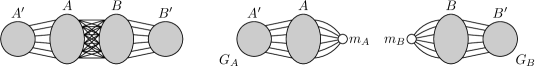
Figure 2: On the left, a split in $G$ between $A$ and $B$. On the right, application of this split produces graphs $G_{A}$ and $G_{B}$ with newly created marker vertices denoted by big white circles.

Split Decomposition and Split Trees.

A split decomposition $D$ of $G$ is a sequence of splits defined as follows. At the beginning, we start with the graph $G$. In the $k$-th step, we have graphs $G_{1},\dots,G_{k}$ and we apply a split on some $G_{i}$, dividing it into two graphs $G^{\prime}_{i}$ and $G^{\prime\prime}_{i}$. The next step then applies to one of the graphs $G_{1},\dots,G_{i-1},G^{\prime}_{i},G^{\prime\prime}_{i},G_{i+1},\dots,G_{k}$, and so on.

A split decomposition can be captured by a graph-labeled tree $T$. The vertices of $T$ are called nodes to distinguish them from the vertices of $G$ and from the added marker vertices, and nodes correspond to subsets of these vertices. To simplify the definition of graph isomorphism of graph-labeled trees, we give a slightly different formal definition in which $T$ is not necessarily a tree.

Definition 2.1.

A graph-labeled tree $T$ is a graph $(V,E)$ with $E=E_{N}\mathbin{\dot{\cup}}E_{T}$ where $E_{N}$ are called the normal edges and $E_{T}$ are called the tree edges. A node is a connected component of $(V,E_{N})$. There are no tree edges between the vertices of one node and no vertex is incident to two tree edges. The incidance graph of nodes must form a tree. The size of $T$ is $|V|+|E|$.

A graph-labeled tree $T$ might not be a tree, but the underlying structure of tree edges forms a tree of nodes. The vertices of $T$ incident to tree edges are called marker vertices.

A split decomposition $D$ of $G$ is represented by the following graph-labeled tree $T$ called the split tree $T$ of $D$ (or a split tree $T$ of $G$). Initially, $T$ consists of a single node equal to $G$. At each step, $D$ applies a split on one node $N$ of $T$. This node is replaced by two new nodes $N_{A}$ and $N_{B}$ while the tree edges incident to $N$ are preserved in $N_{A}$ and $N_{B}$ and the marker vertices $m_{A}$ and $m_{B}$ are further adjacent by a newly formed tree edge. Figure 3 shows an example. It can be observed that the total size of every split tree is ${\mathcal{O}}(n+m)$ where $n$ is the number of vertices and $m$ is the number of edges of the original graph.

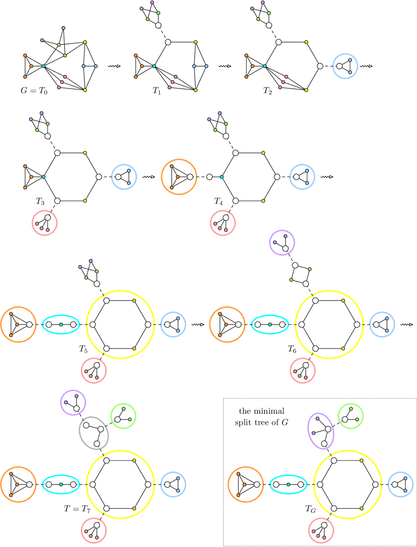
Figure 3: An example of a split tree $T$ of a split decomposition $D$ ending with highlighted prime and degenerate graphs (see the definition below). The split decomposition $D$ is not minimal: the gray and purple stars can be joined in $T$ to form the minimal split tree $T_{G}$ in the box.

From a split tree $T$, the original graph $G$ can be reconstructed by joining neighboring nodes. For a tree edge $m_{A}m_{B}$, we remove $m_{A}$ and $m_{B}$ while adding all edges $uv$ for $u\in N(m_{A})$ and $v\in N(m_{B})$.

Recognition of Circle Graphs.

A split decomposition can be applied to recognize circle graphs. The key is the following observation.

Lemma 2.2.

A graph is a circle graph if and only if both $G_{A}$ and $G_{B}$ are circle graphs.

The proof is illustrated in Figure 4, which can be easily formalized; see for example [43]. A prime circle graph has a unique circle representation up to reversal [13] which can be constructed in polynomial time [20].

Figure 4: On the left, circle representations ${\mathcal{R}}_{A}$ and ${\mathcal{R}}_{B}$ of graphs $G_{A}$ and $G_{B}$. They are combined into a circle representation ${\mathcal{R}}$ of $G$.

Minimal Split Decomposition.

A graph is called degenerate if it is the complete graph $K_{n}$ or the star $S_{n}$. Suppose that we have a split decomposition $D$ ending on prime graphs. Its split tree is not uniquely determined, for instance degenerate graphs have many different split trees. Cunnigham [10] resolved this issue by terminating the split decomposition not only on prime graphs, but also on the degenerate graphs.

Cunnigham [10] introduced the notion of a minimal split decomposition. A split decomposition is minimal if the corresponding split tree has all nodes as prime and degenerate graphs, and joining any two neighboring nodes creates a non-degenerate graph.

Theorem 2.3 (Cunningham [10], Theorem 3).

For a connected graph $G$, the split tree of a minimal split decomposition terminating on prime and degenerate graphs is uniquely determined.

The split tree of a minimal split decomposition of $G$ is called the minimal split tree of $G$ and it is denoted $T_{G}$.

It was stated in [21, Theorem 2.17] that a split decomposition is minimal if the corresponding split tree has no two neighboring nodes such that

• either both are complete,

• or both are stars and the tree edge joining these stars is incident to exactly one of their central vertices.

The reason is that such neighboring nodes can be joined into a complete node or a star node, respectively. Therefore, the minimal split tree can be constructed from an arbitrary split tree by joining neighboring complete graphs and stars. For instance, the split tree $T$ in Fig. 3 is not minimal since the purple and gray stars can be joined, creating the minimal split tree $T_{G}$.

Cunnigham’s definition of a minimal split decomposition is with respect to inclusion. Since the minimal split decomposition is uniquely determined, it is equivalently the split decomposition terminating on prime and degenerate graphs using the least number of splits.

Computation of Minimal Split Trees.

The minimal split tree can be computed in time ${\mathcal{O}}(n+m)$ using the algorithm of [13]. For the purpose of this paper, we use the following slower algorithm since it also computes the unique circle representations of encountered prime circle graphs:

Theorem 2.4 (Gioan et al. [21, 20]).

The minimal split tree $T_{G}$ of a circle graph $G$ can be computed in time ${\mathcal{O}}((n+m)\cdot\alpha(n+m))$ where $n$ is the number of vertices, $m$ is the number of edges, and $\alpha$ is the inverse Ackermann function. Further, the algorithm also computes the unique circle representation of each prime circle node of $T_{G}$.

Graph Isomorphism Via Minimal Split Decompositions.

Let $T$ and $T^{\prime}$ be two graph-labeled trees. An isomorphism $\pi:T\to T^{\prime}$ is an isomorphism which maps normal edges to normal edges and tree edges to tree edges. Notice that $\pi$ maps nodes of $T$ to isomorphic nodes of $T^{\prime}$ while preserving tree edges.

We use minimal split trees to test graph isomorphism of circle graphs:

Lemma 2.5.

Two connected graphs $G$ and $H$ are isomorphic if and only if the minimal split trees $T_{G}$ and $T_{H}$ are isomorphic.

Proof.

Let $T^{\prime}_{G}$ and $T^{\prime}_{H}$ be any split trees of $G$ and $H$, respectively, and $\pi:T^{\prime}_{G}\to T^{\prime}_{H}$ be an isomorphism. We want to show that $G\cong H$. Choose an arbitrary tree edge $e=m_{A}m_{B}$ in $T^{\prime}_{G}$, we know that $\pi(e)=\pi(m_{A})\pi(m_{B})$ is a tree edge in $T^{\prime}_{H}$. We join $T^{\prime}_{G}$ over $e$ and $T^{\prime}_{H}$ over $\pi(e)$. We get that the restriction $\pi|_{T^{\prime}_{G}\setminus\{m_{A},m_{B}\}}$ is an isomorphism of the constructed graph-labeled trees. By repeating this process, we get single nodes isomorphic graph-labeled trees which are $G$ and $H$ respectively. So $G\cong H$.

For the other implication, suppose that $\pi:G\to H$ is an isomorphism. Let $D_{G}$ be a minimal split decomposition, constructing the minimal split tree $T_{G}$. We use $\pi$ to construct a split decomposition $D_{H}$ and a split tree $T_{H}$ of $H$ such that $T_{G}\cong T_{H}$. Before any splits, the trees $T_{G}^{0}\cong G$ and $T_{H}^{0}\cong H$ are isomorphic. Suppose that $T_{G}^{k}\cong T_{H}^{k}$ and $D_{G}$ then uses a split between $A$ and $B$ in some node $N$. Then $D_{H}$ will use the split between $\pi(A)$ and $\pi(B)$, and since $\pi$ is an isomorphism, it is a valid split in $\pi(N)$. We construct $T_{G}^{k+1}$ by splitting $N$ into two nodes $N_{A}$ and $N_{B}$ and adding marker vertices $m_{A}$ and $m_{B}$, and similarly for $T_{H}^{k+1}$ with marker vertices $m_{\pi(A)}$ and $m_{\pi(B)}$. We extend $\pi$ to an isomorphism from $T_{G}^{k+1}$ to $T_{H}^{k+1}$ by setting $\pi(m_{A})=m_{\pi(A)}$ and $\pi(m_{B})=m_{\pi(B)}$. Therefore, the resulting split trees $T_{G}$ and $T_{H}$ are isomorphic. By Theorem 2.3, the minimal split tree of $H$ is uniquely determined, so it has to be isomorphic to the constructed $T_{H}$. ∎

3 Canonization of Graph-labeled Trees

In the rest of the paper, we work with colored graphs and isomorphisms are required to be color-preserving. Colors are represented as non-negative integers.

Definition of Canonization.

Let $G$ be a colored graph with $n$ vertices with colors in the range $0,\dots,n-1$ and $m$ edges. An encoding $\varepsilon(G)$ of $G$ is a sequence of non-negative integers. The encoding $\varepsilon(G)$ is linear if it contains at most ${\mathcal{O}}(n+m)$ integers, each in range $0,\dots,n-1$. We denote the class of all encodings by ${\mathcal{E}}$. For a class of graphs ${\mathcal{C}}$, a linear canonization is some function $\gamma:{\mathcal{C}}\to{\mathcal{E}}$ such that $\gamma(G)$ is a linear encoding of $G$ and for $G,H\in{\mathcal{C}}$, we have $G\cong H$ if and only if $\gamma(G)=\gamma(H)$.

Fast Lexicographic Sorting.

Since we want to sort these encodings lexicographically, we frequently use the following well-known algorithm:

Lemma 3.1 (Aho, Hopcroft, and Ullman [1], Algorithm 3.2, p. 80).

It is possible to lexicographically sort sequences of numbers $0,\dots,t-1$ of arbitrary lengths in time ${\mathcal{O}}(\ell+t)$ where $\ell$ is the total length of these sequences.

It is easy to modify the above algorithm to get the same running time when all numbers belong to $\{0,1,2,\dots,t+1,s,s+1,\dots,s+t-1\}$.

Canonization Algorithm.

In the rest of this section, we are going to describe the following meta-algorithm.

Lemma 3.2.

Let ${\mathcal{C}}$ be a class of graphs and ${\mathcal{T}}$ be a class of graph-labeled trees whose nodes belong to ${\mathcal{C}}$. Suppose that we can compute a linear-space canonization $\gamma$ of colored graphs in ${\mathcal{C}}$ in time $f(n+m)$ where $n$ is the number of vertices, $m$ is the number of edges, and $f$ is convex. Then we can compute a linear-space canonization $\widetilde{\gamma}$ of graph-labeled trees from ${\mathcal{T}}$ in time ${\mathcal{O}}(n+m+f(n+m))$.

Let $T\in{\mathcal{T}}$ be a graph-labeled tree. We may assume that $T$ is rooted at the central node. If a tree edge is central, we insert there another node having a single vertex. Also, we orient all tree edges towards the root. For a node $N$, we denote by $T[N]$ the graph-labeled subtree induced by $N$ and all descendants of $N$. Initially, we color all marker vertices by the color $0$ and all other vertices by the color $1$. Throughout the algorithm, only marker vertices change colors.

The $k$-th layer in $T$ is formed by all nodes of the distance $k$ from the root. Notice that every isomorphism from $T$ to $T^{\prime}$ maps, for every $k$, the $k$-th layer of $T$ to the $k$-th layer of $T^{\prime}$. Also, every node $N$ aside the root is incident to exactly one out-going tree edge whose incident marker vertex outside $N$ is called the parent marker vertex of $N$.

The algorithm starts from the bottom layer of $T$ and process the layers towards the root. When a node $N$ is processed, we assign a color $c$ to $N$. This color $c$ corresponds to a certain linear encoding $\gamma^{\prime}(N)$ which is created by modifying $\gamma(N)$. Further, we store the mapping $\varepsilon$ from colors to these linear encodings, so $\varepsilon(c)=\gamma^{\prime}(N)$. The assigned colors have the property that two nodes $N$ and $N^{\prime}$ have the same assigned color if and only if the rooted graph-labeled subtrees induced by $N$ and all the nodes below and by $N^{\prime}$ and all the nodes below, respectively, are isomorphic. We remove the node $N$ from $T$ and assign its color to the parent marker vertex of $N$. Also notice that when a non-root node is processed, all marker vertices except for one have colors different from $0$, and for the root node, all marker vertices have colors different from $0$.

Let $N_{1},\dots,N_{k}$ be the nodes of the currently processed layer such that each vertex in these nodes has one color from $\{0,1,s,s+1,\dots,s+t-1\}$. For each node $N_{i}$, we want to use the canonization subroutine to compute the linear encoding $\gamma(N_{i})$. But the assumptions require that for $\ell$ vertices in $N_{i}$, all colors are in range $0,\dots,\ell-1$, but we might have $s\gg\ell$. We can avoid this by renumbering the colors since at most $\ell$ different colors are used on $N_{i}$. Suppose that exactly $c_{i}$ different colors are used in $N_{i}$, and we define the injective mapping $\varphi_{N_{i}}:\{0,1,\dots,c_{i}-1\}\to\{0,1,s,s+1,\dots,s+t-1\}$ such that the smallest used color is $\varphi_{N_{i}}(0)$, the second smallest is $\varphi_{N_{i}}(1)$, and so on till $\varphi_{N_{i}}(c_{i}-1)$. The renumbering of colors on $N_{i}$ is given by the inverse $\varphi_{N_{i}}^{-1}$.

After renumbering, the algorithm runs the canonization subroutine to compute the linear encodings $\gamma(N_{1}),\dots,\gamma(N_{k})$. We create the modified linear encoding $\gamma^{\prime}(N_{i})$ by pre-pending $\gamma(N_{i})$ with the sequence $c_{i}$, $\varphi_{N_{i}}(0)$, $\varphi_{N_{i}}(1)$, …, $\varphi_{N_{i}}(c_{i}-1)$ where $c_{i}$ is the number of different colors used in $N_{i}$. The algorithm lexicographically sorts these modified encodings $\gamma^{\prime}(N_{1}),\dots,\gamma^{\prime}(N_{k})$ using Lemma 3.1. Next, we assign the color $s+t$ to the nodes having the smallest encodings, the color $s+t+1$ to the nodes having the second smallest encodings, and so on. For every node $N_{i}$, we remove it and set the color of the parent marker vertex of $N_{i}$ to the color assigned to $N_{i}$.

Suppose that the root node $N$ has the color $c$ assigned, so throughout the algorithm, we have used the colors $0,\dots,c$. The computed linear encoding of $T$ is an encoded concatenation of $\varepsilon(2),\varepsilon(3),\dots,\varepsilon(c)$.

Lemma 3.3.

The described algorithm produces a correct linear canonization $\widetilde{\gamma}$ of graph-labeled trees in ${\mathcal{T}}$, i.e., for $T,T^{\prime}\in{\mathcal{T}}$, we have $T\cong T^{\prime}$ if and only if $\widetilde{\gamma}(T)=\widetilde{\gamma}(T^{\prime})$.

Proof.

Let $\pi:T\to T^{\prime}$ be an isomorphism. We prove by induction from the bottom layer to the root that $\gamma^{\prime}(N)=\gamma^{\prime}(\pi(N))$. Suppose that we are processing the $\ell$-th layer of $T$ and $T^{\prime}$ and all previously used colors have the same assigned encodings in $T$ and $T^{\prime}$. For every node $N$ of the $\ell$-th layer of $T$, then $\pi(N)$ belongs to the $\ell$-th layer of $T^{\prime}$. We argue that $\pi$ also preserves the colors of $N$. Since $\pi$ is an isomorphism of graph-labeled trees, it maps marker vertices to marker vertices and non-marker vertices to non-marker vertices. Let $N_{1},\dots,N_{k}$ be the children of $N$. By the induction hypothesis, we have $\gamma^{\prime}(N_{i})=\gamma^{\prime}(\pi(N_{i}))$, so the same colors are assigned to $N_{i}$ and $\pi(N_{i})$. Therefore, $\pi$ preserves the colors of $N$, and this property still holds after renumbering the colors by $\varphi_{N}^{-1}=\varphi_{\pi(N)}^{-1}$. Therefore, we have $\gamma(N)=\gamma(\pi(N))$ and thus $\gamma^{\prime}(N)=\gamma^{\prime}(\pi(N))$. Thus, the lexicographic sorting of the nodes in the $\ell$-th layer of $T$ and of $T^{\prime}$ is the same, so $N$ and $\pi(N)$ have the same color assigned. Finally, the encodings $\varepsilon(2),\dots,\varepsilon(c)$ are the same in $T$ and $T^{\prime}$, so $\widetilde{\gamma}(T)=\widetilde{\gamma}(T^{\prime})$.

For the other implication, we show that a graph-labeled tree $T^{\prime}$ isomorphic to $T$ can be reconstructed from $\widetilde{\gamma}(T)$. We construct the root node $N$ from $\varepsilon(c)$. Since $\gamma$ is a canonization of ${\mathcal{C}}$, we obtain $N$ by applying $\gamma^{-1}$. Next, we invert the recoloring by applying $\varphi(N)$ on the colors of $N$. Next, we consider each marker vertex in $N$. If it has some color $c_{i}$, we use $\varepsilon(c_{i})$ to construct a child node $N^{\prime}$ of $N$ exactly as before. We proceed in this way till all nodes are expanded and only the colors $0$ and $1$ remain. It is easy to prove by induction that $T\cong T^{\prime}$ since each $\varepsilon(c_{i})$ uniquely determines the corresponding subtree in $T$. ∎

Lemma 3.4.

The described algorithm runs in time ${\mathcal{O}}(n+m+f(n+m))$.

Proof.

When we run the canonization subroutine on a node having $n^{\prime}$ vertices and $m^{\prime}$ edges, it has all colors in range $0,\dots,n^{\prime}-1$, so we can compute its linear encoding in time $f(n^{\prime}+m^{\prime})$. Since $f$ is convex and the canonization subroutine runs on each node exactly once, the total time spend by this subroutine is bounded by $f(n+m)$.

The total count of used colors is clearly bounded by $n$ and each layer uses different colors except for $0$ and $1$. Consider a layer with nodes $N_{1},\dots,N_{k}$ having $\ell$ vertices and $\ell^{\prime}$ edges in total. All these nodes use at most $\ell$ different colors. Therefore, the modified encodings $\gamma^{\prime}(N_{1}),\dots,\gamma^{\prime}(N_{k})$ consisting of integers from $\{0,1,2,\dots,\ell+1,s,s+1,\dots,s+\ell-1\}$, for some value $s$, and are of the total length ${\mathcal{O}}(\ell+\ell^{\prime})$. Therefore, lexicografic sorting of these modified encodings can be done in time ${\mathcal{O}}(\ell+\ell^{\prime})$, and this sorting takes total time ${\mathcal{O}}(n+m)$ for all layers of $T$. Therefore, the total running time of the algorithm is ${\mathcal{O}}(n+m+f(n+m))$. ∎

Proof of Lemma 3.2.

It follows by Lemmas 3.3 and 3.4. ∎

4 Canonization of Prime and Degenerate Circle Graphs

Let ${\mathcal{C}}$ be the class of colored prime and degenerate circle graphs. Recall that all nodes of minimal split trees of connected circle graphs belong to ${\mathcal{C}}$. To apply the meta-algorithm of Lemma 3.2, we need to show that the linear canonization $\gamma$ of ${\mathcal{C}}$ can be computed in time ${\mathcal{O}}(n+m)$ where $n$ is the number of vertices and $m$ is the number of edges.

Linear Canonizations of Degenerate Graphs.

For a colored complete graph $G=K_{n}$, we sort its colors using bucket sort in time ${\mathcal{O}}(n)$, so the vertices have the colors $c_{1}\leq c_{2}\leq\dots\leq c_{n}$. The computed linear canonization $\gamma(G)$ is $0,c_{1},c_{2},\dots,c_{n}$.

For a star $G=S_{n}$, we sort the colors of leaves using bucket sort in time ${\mathcal{O}}(n)$, so they have the colors $c_{1}\leq c_{2}\leq\dots\leq c_{n}$, while the center has the color $c_{0}$. The computed linear canonization $\gamma(G)$ is $1,c_{0},c_{1},c_{2},\dots,c_{n}$.

Linear Encodings of Colored Cycles.

As a subroutine, we need to find a canonical form of a colored cycle. To do this, it suffices to find the the lexicographically minimal rotation of a circular string. This can be done using ${\mathcal{O}}(n)$ comparisons over some alphabet $\Sigma$ [4, 41].

Linear Canonizations of Circle Representations.

Let $G$ be an arbitrary colored circle graph on $n$ vertices together with an arbitrary circle representation ${\mathcal{R}}$. The standard way to describe ${\mathcal{R}}$ is to arbitrarily order the vertices $1,\dots,n$ and to give a circular word $\omega$ consisting of $2n$ integers from $1,\dots,n$, each appearing exactly twice, in such a way that the occurrences of $i$ and $j$ alternate (i.e., appear as $ijij$) if and only if $ij\in E(G)$. This circular word describes the ordering of endpoint of the chords in, say, the clockwise direction.

Let $G$ and $H$ be two colored circle graphs on $n$ vertices labeled $1,\dots,n$ with circle representations ${\mathcal{R}}_{G}$ and ${\mathcal{R}}_{H}$ represented by $\omega_{G}=\omega_{G}^{1},\dots,\omega_{G}^{2n}$ and $\omega_{H}=\omega_{H}^{1},\dots,\omega_{H}^{2n}$. We say that ${\mathcal{R}}_{G}\cong{\mathcal{R}}_{H}$ if and only if there exists a bijection $\pi:\{1,\dots,n\}\to\{1,\dots,n\}$ such that

• the vertices $i$ in $G$ and $\pi(i)$ in $H$ have identical colors, and

• the circular words $\omega_{H}$ and $\pi(\omega_{G}^{1}),\dots,\pi(\omega_{G}^{2n})$ are identical.

Notice that when ${\mathcal{R}}_{G}\cong{\mathcal{R}}_{H}$, necessarily $G\cong H$, but in general the converse is not true. We want to construct a linear canonization $\gamma$ such that ${\mathcal{R}}_{G}\cong{\mathcal{R}}_{H}$ if and only if $\gamma({\mathcal{R}}_{G})=\gamma({\mathcal{R}}_{H})$.

We want to construct $\gamma({\mathcal{R}}_{G})$ directly from the representation but an arbitrary chosen labeling of vertices in $\omega_{G}$ is not helpful. Therefore, we consider a different encoding of the representation which is invariant on rotation. For each of $2n$ endpoints $e_{1},\dots,e_{2n}$, we store two numbers:

• The color $c_{i}\in\{0,\dots,n-1\}$ of the vertex of the chord corresponding to $e_{i}$.

• The number of endpoints $g_{i}$ in the clockwise direction between $e_{i}$ and the other endpoint corresponding to the same chord. We have $g_{i}\in\{0,\cdots,2n-2\}$ and when the $e_{i}$ and $e_{j}$ correspond one chord, then $g_{i}+g_{j}=2n-2$.

To distinguish $c_{i}$ from $g_{i}$, we increase all $c_{i}$ by $2n-1$, so $c_{i}\in\{2n-1,\cdots,3n-2\}$. Then we may consider the circular word $\lambda_{G}=g_{1},c_{1},g_{2},c_{2},\dots,g_{2n},c_{2n}$ of length $4n$.

Lemma 4.1.

Let $G$ and $H$ be two colored circle graphs with representations ${\mathcal{R}}_{G}$ and ${\mathcal{R}}_{H}$. We have ${\mathcal{R}}_{G}\cong{\mathcal{R}}_{H}$ if and only if the circular words $\lambda_{G}$ and $\lambda_{H}$ are identical.

Proof.

If ${\mathcal{R}}_{G}\cong{\mathcal{R}}_{H}$, there exists an index $k\in\{0,\dots,2n-1\}$ such that rotating the representation ${\mathcal{R}}_{G}$ by $k$ endpoints produces ${\mathcal{R}}_{H}$. When $\lambda_{G}=g_{1},c_{1},\dots,g_{2n},c_{2n}$ and $\lambda_{H}=g^{\prime}_{1},c^{\prime}_{1},\dots,g^{\prime}_{2n},c^{\prime}_{2n}$, it cyclically holds that $g_{i}=g^{\prime}_{i+k}$ and $c_{i}=c^{\prime}_{i+k}$. So the circular words $\lambda_{G}$ and $\lambda_{H}$ are identical.

For the other implication, observe that the circle representation ${\mathcal{R}}_{G}$ and the circle graph $G$ can be reconstructed from $\lambda_{G}$. If $\lambda_{G}$ and $\lambda_{H}$, we reconstruct isomorphic representations ${\mathcal{R}}_{G}$ and ${\mathcal{R}}_{H}$. ∎

Lemma 4.2.

We can compute the linear encoding $\gamma$ of colored circle representations in time ${\mathcal{O}}(n)$.

Proof.

For a representation ${\mathcal{R}}_{G}$, we can clearly compute $\lambda_{G}$ in time ${\mathcal{O}}(n)$. Next, we apply to $\lambda_{G}$ an cycle canonization algorithm [4, 41] which computes $\gamma({\mathcal{R}}_{G})$ in time ${\mathcal{O}}(n)$. ∎

Linear Canonization of Prime Circle Graphs.

Let $G$ be a prime circle graph. It has at most two different representations ${\mathcal{R}}_{G}$ and ${\mathcal{R}}^{\prime}_{G}$ where one is the reversal of the other. Using Lemma 4.2, we compute their linear encodings $\lambda_{G}$ and $\lambda^{\prime}_{G}$. As the linear encoding $\gamma(G)$, we chose the lexicographically smallest of $\lambda_{G}$ and $\lambda^{\prime}_{G}$, prepended with the value $2$. Clearly, colored prime circle graphs $G$ and $H$ are isomorphic if and only if $\gamma(G)=\gamma(H)$.

By putting the results of this section together, we get the following:

Lemma 4.3.

We can compute linear canonization of colored prime circle graphs and degenerate graphs in time ${\mathcal{O}}(n)$.

5 Canonization and Graph Isomorphism of Circle Graphs

In this section, we combine the presented results to show that a linear canonization $\gamma$ of circle graphs can be computed in time ${\mathcal{O}}((n+m)\cdot\alpha(n+m))$. This algorithm clearly implies Theorem 1.1 since circle graphs $G$ and $H$ are isomorphic if and only if $\gamma(G)=\gamma(H)$.

Suppose that $G$ is a connected circle graph. We apply the algorithm of Theorem 2.4 to compute the minimal split decomposition $T_{G}$ of $G$ and the unique circle representation for each prime circle graph (up to reversal). We halt if some circle representations does not exist since $G$ is not a circle graph. The total running time of preprocessing is ${\mathcal{O}}((n+m)\cdot\alpha(n+m))$, and the remainder of the algorithm runs in time ${\mathcal{O}}(n+m)$, so this step is the bottleneck. Next, we use Lemmas 4.3 and 3.2 to compute a linear canonization $\gamma(T_{G})$ and we put $\gamma(G)=\gamma(T_{G})$.

Suppose that the circle graph $G$ is disconnected, and let $G_{1},\dots,G_{k}$ be its connected components. We compute their linear encodings $\gamma(G_{1}),\dots,\gamma(G_{k})$, lexicografically sort them in time ${\mathcal{O}}(n+m)$ using Lemma 3.1, and output them in $\gamma(G)$ sorted as a sequence. The total running time is ${\mathcal{O}}((n+m)\cdot\alpha(n+m))$.

When the input also gives a circle representation ${\mathcal{R}}$, we can avoid using Theorem 2.4. Instead, we compute a split decomposition and the corresponding split tree in time ${\mathcal{O}}(n+m)$ using [13]. We can easily modify this split tree into the minimal split tree by joining neighboring complete vertices and stars as discussed in Section 2. For each prime node $N$, we obtain its unique circle representation by restricting ${\mathcal{R}}$ to the vertices of $N$. Since the avoided algorithm of Theorem 2.4 was the bottleneck, we get the total running time ${\mathcal{O}}(n+m)$.

6 Conclusions

We conclude this paper by discussing several possible research directions and open problems. The main used tool is minimal split decomposition. The algorithm finds the cannonical form of the unique minimal split tree $T$, using the canonical forms of every prime and degenerate circle graph appearing as a node of $T$. We obtain an algorithm computing the cannonical form for every circle graph.

Problem 6.1.

Does the minimal split tree capture all possible representations of circle graph?

The $k$-dimensional Weisfeiler-Leman [44] algorithm ($k$-dim WL) is a fundamental algorithm used as a subroutine in graph isomorphism testing. The algorithm colors $k$-tuples of vertices of two input graphs and iteratively refines the color classes until the coloring becomes stable. We say that $k$-dim WL distinguishes two graph $G$ and $H$ if and only if its application to each of them gives colorings with different sizes of color classes. Two distinguished graphs are clearly non-isomorphic, however, for every $k$, there exist non-isomorphic graphs not distinguished by $k$-dim WL. For a class of graphs ${\mathcal{C}}$, the Weisfeiler-Leman dimension of ${\mathcal{C}}$ is the minimum integer $k$ such that $k$-dim WL distinguishes every $G,H\in{\mathcal{C}}$ such that $G\not\cong H$.

Problem 6.2.

What is the Weisfeiler-Leman dimension of circle graphs?

For many classes of graphs, such as trees, interval graphs [16], planar graphs [26], or more generally graphs with excluded minors [22], and recently also circular-arc graphs [38], the Weisfeiler-Leman dimension is finite. A major open problem is for which classes of graphs can isomorphism be tested in polynomial time without using group theory, i.e., by a combinatorial algorithm, often meant some $k$-dim WL.

Further, a natural question to ask, especially for problems solvable in linear time, is whether they can be solved using logarithmic space. This is, for example, known for interval graphs [32] and Helly circular-arc graphs [33]. Recently, a parametrized logspace algorithm was given for circular-arc graphs in [7].

Problem 6.3.

Can isomorphism of circle graphs be tested using logarithmic space?

Finally, we mention the partial representation extension problem which is a generalization of the recognition problem. The input consists of, in our case, a circle graph and a circle representation of its induced subgraph and the task is to complete the representation or output that it is not possible. Obviously, this problem can be asked for various classes of graphs and it was extensively studied [30, 28, 29, 8, 3, 34].

In [8], the authors give an ${\mathcal{O}}(n^{3})$ algorithm to solve this problem. They give an elementary recursive description of the structure of all representations and try to match the partial representation on it. It is a natural question whether the minimal split trees can be used to solve the partial representation extension problem faster.

Problem 6.4.

Can the partial representation extension problem for circle graphs be solved using minimal split decomposition faster that ${\mathcal{O}}(n^{3})$?

References

- [1] A. V. Aho, J. E. Hopcroft, and J. D. Ullman. The Design and Analysis of Computer Algorithms. Addison-Wesley Publishing Company, 1974.
- [2] L. Babai. Graph isomorphism in quasipolynomial time. In STOC, 2016.
- [3] J. Bang-Jensen, J. Huang, and X. Zhu. Completing orientations of partially oriented graphs. CoRR, abs/1509.01301, 2015.
- [4] Kellogg S Booth. Lexicographically least circular substrings. Information Processing Letters, 10(4-5):240–242, 1980.
- [5] A. Bouchet. Reducing prime graphs and recognizing circle graphs. Combinatorica, 7(3):243–254, 1987.
- [6] A. Bouchet. Unimodularity and circle graphs. Discrete Mathematics, 66(1-2):203–208, 1987.
- [7] Maurice Chandoo. Deciding circular-arc graph isomorphism in parameterized logspace. In 33rd Symposium on Theoretical Aspects of Computer Science (STACS 2016). Schloss Dagstuhl-Leibniz-Zentrum fuer Informatik, 2016.
- [8] S. Chaplick, R. Fulek, and P. Klavík. Extending partial representations of circle graphs. CoRR, abs/1309.2399, 2015.
- [9] C. J. Colbourn. On testing isomorphism of permutation graphs. Networks, 11(1):13–21, 1981.
- [10] William H Cunningham. Decomposition of directed graphs. SIAM Journal on Algebraic Discrete Methods, 3(2):214–228, 1982.
- [11] William H Cunningham and Jack Edmonds. A combinatorial decomposition theory. Canadian Journal of Mathematics, 32(3):734–765, 1980.
- [12] A. R. Curtis, M. C. Lin, R. M. McConnell, Y. Nussbaum, F. J. Soulignac, J. P. Spinrad, and J. L. Szwarcfiter. Isomorphism of graph classes related to the circular-ones property. Discrete Mathematics and Theoretical Computer Science, 15(1):157–182, 2013.
- [13] E. Dahlhaus. Parallel algorithms for hierarchical clustering and applications to split decomposition and parity graph recognition. Journal of Algorithms, 36(2):205–240, 1998.
- [14] H. de Fraysseix. Local complementation and interlacement graphs. Discrete Mathematics, 33(1):29–35, 1981.
- [15] H. de Fraysseix and P. O. de Mendez. On a characterization of gauss codes. Discrete & Computational Geometry, 22(2):287–295, 1999.
- [16] Sergei Evdokimov, Ilia Ponomarenko, and Gottfried Tinhofer. Forestal algebras and algebraic forests (on a new class of weakly compact graphs). Discrete Mathematics, 225(1-3):149–172, 2000.
- [17] S. Even and A. Itai. Queues, stacks, and graphs. Theory of Machines and Computation (Z. Kohavi and A. Paz, Eds.), pages 71–76, 1971.
- [18] J. Fiala, P. Klavík, J. Kratochvíl, and R. Nedela. 3-connected reduction for regular graph covers. CoRR, abs/1503.06556, 2017.
- [19] C. P. Gabor, K. J. Supowit, and W. Hsu. Recognizing circle graphs in polynomial time. J. ACM, 36(3):435–473, 1989.
- [20] E. Gioan, C. Paul, M. Tedder, and D. Corneil. Practical and efficient circle graph recognition. Algorithmica, 69(4):759–788, 2014.
- [21] E. Gioan, C. Paul, M. Tedder, and D. Corneil. Practical and efficient split decomposition via graph-labelled trees. Algorithmica, 69(4):789–843, 2014.
- [22] Martin Grohe. Descriptive complexity, canonisation, and definable graph structure theory, volume 47. Cambridge University Press, 2017.
- [23] J. E. Hopcroft and J. Wong. Linear time algorithm for isomorphism of planar graphs. In STOC, pages 172–184. ACM, 1974.
- [24] W. L. Hsu. algorithms for the recognition and isomorphism problems on circular-arc graphs. SIAM Journal on Computing, 24(3):411–439, 1995.
- [25] K. Kawarabayashi, P. Klavík, B. Mohar, R. Nedela, and P. Zeman. Isomorphisms of maps on the sphere. to appear in Contemporary Mathematics AMS, 2019.
- [26] Sandra Kiefer, Ilia Ponomarenko, and Pascal Schweitzer. The weisfeiler-leman dimension of planar graphs is at most 3. In 2017 32nd Annual ACM/IEEE Symposium on Logic in Computer Science (LICS), pages 1–12. IEEE, 2017.
- [27] P. Klavík, D. Knop, and P. Zeman. Graph isomorphism restricted by lists. CoRR, abs/1607.03918, 2016.
- [28] P. Klavík, J. Kratochvíl, Y. Otachi, I. Rutter, T. Saitoh, M. Saumell, and T. Vyskočil. Extending partial representations of proper and unit interval graphs. Algorithmica, 77(4):1071–1104, 2017.
- [29] P. Klavík, J. Kratochvíl, Y. Otachi, and T. Saitoh. Extending partial representations of subclasses of chordal graphs. Theoretical Computer Science, 576:85–101, 2015.
- [30] P. Klavík, J. Kratochvíl, Y. Otachi, T. Saitoh, and T. Vyskočil. Extending partial representations of interval graphs. Algorithmica, 2016.
- [31] P. Klavík and P. Zeman. Automorphism groups of geometrically represented graphs. In 32nd International Symposium on Theoretical Aspects of Computer Science, STACS 2015, volume 30 of Leibniz International Proceedings in Informatics (LIPIcs), pages 540–553, 2015.
- [32] Johannes Köbler, Sebastian Kuhnert, Bastian Laubner, and Oleg Verbitsky. Interval graphs: Canonical representations in logspace. SIAM Journal on Computing, 40(5):1292–1315, 2011.
- [33] Johannes Köbler, Sebastian Kuhnert, and Oleg Verbitsky. Helly circular-arc graph isomorphism is in logspace. In International Symposium on Mathematical Foundations of Computer Science, pages 631–642. Springer, 2013.
- [34] T. Krawczyk and B. Walczak. Extending partial representations of trapezoid graphs. In WG 2017, Lecture Notes in Computer Science, 2017.
- [35] Min Chih Lin, Francisco J Soulignac, and Jayme L Szwarcfiter. A simple linear time algorithm for the isomorphism problem on proper circular-arc graphs, 2008.
- [36] G. S. Lueker and K. S. Booth. A linear time algorithm for deciding interval graph isomorphism. Journal of the ACM (JACM), 26(2):183–195, 1979.
- [37] W. Naji. Graphes de Cordes: Une Caracterisation et ses Applications. PhD thesis, l’Université Scientifique et Médicale de Grenoble, 1985.
- [38] Roman Nedela, Ilia Ponomarenko, and Peter Zeman. Testing isomorphism of circular-arc graphs in polynomial time. arXiv preprint arXiv:1903.11062, 2019.
- [39] S. Oum. Rank-width and vertex-minors. J. Comb. Theory, Ser. B, 95(1):79–100, 2005.
- [40] U. Schöning. Graph isomorphism is in the low hierarchy. Journal of Computer and System Sciences, 37(3):312–323, 1988.
- [41] Yossi Shiloach. Fast canonization of circular strings. Journal of algorithms, 2(2):107–121, 1981.
- [42] J. P. Spinrad. Recognition of circle graphs. J. of Algorithms, 16(2):264–282, 1994.
- [43] J. P. Spinrad. Efficient Graph Representations. Field Institute Monographs, 2003.
- [44] B. Weisfeiler and A.A. Leman. A reduction of a graph to a canonical form and an algebra arising during this reduction. Nauchno-Technicheskaya Informatsiya, 9:12–16, 1968.