Global Solar Magnetic-field and Interplanetary Scintillations During the Past Four Solar Cycles

Abstract

The extended minimum of Solar Cycle 23, the extremely quiet solar-wind conditions prevailing and the mini-maximum of Solar Cycle 24 drew global attention and many authors have since attempted to predict the amplitude of the upcoming Solar Cycle 25, which is predicted to be the third successive weak cycle; it is a unique opportunity to probe the Sun during such quiet periods. Earlier work has established a steady decline, over two decades, in solar photospheric fields at latitudes above $45^{\circ}$ and a similar decline in solar-wind micro-turbulence levels as measured by interplanetary scintillation (IPS) observations. However, the relation between the photospheric magnetic-fields and those in the low corona/solar-wind are not straightforward. Therefore, in the present article, we have used potential-field source-surface (PFSS) extrapolations to deduce global magnetic-fields using synoptic magnetograms observed with National Solar Observatory (NSO), Kitt Peak, USA (NSO/KP) and Solar Optical Long-term Investigation of the Sun (NSO/SOLIS) instruments during 1975 –  2018. Furthermore, we have measured the normalized scintillation index [m] using the IPS observations carried out at the Institute of Space Earth Environment Research (ISEE), Japan during 1983 –  2017. From these observations, we have found that, since the mid 1990s, the magnetic-field over different latitudes at 2.5 $\rm R_{\odot}$ and 10 $\rm R_{\odot}$(extrapolated using PFSS method) has decreased by $\approx 11.3-22.2\,\%$. In phase with the declining magnetic-fields, the quantity m also declined by $\approx 23.6\,\%$. These observations emphasize the inter-relationship among the global magnetic-field and various turbulence parameters in the solar corona and solar-wind.

1 Introduction

The magnetic-field plays a crucial role in understanding the various phenomenon that occur on the Sun and solar atmosphere. Most of the features (e.g. sunspots, filaments, prominences, coronal holes) and transient events (e.g. solar flares, coronal mass ejections, and non-thermal radio bursts) are related to magnetic-field. Recent work has established a steady decline, over the past two decades, in solar photospheric fields at latitudes above $45^{\circ}$ and a similar decline in solar-wind micro-turbulence levels as measured by interplanetary scintillation (IPS) observations (Janardhan et al., 2010, 2011, 2015). Solar cycle 24 has also shown a significant asymmetry in the times of reversals of the polar field in the two solar hemispheres (Janardhan et al., 2018), leading to speculation as to whether we are heading towards a another Grand solar minimum like the Maunder minimum if the decline in the photospheric fields will continue beyond 2020, the expected minimum of the current Solar Cycle 24.

Although photospheric magnetic-fields is available from many decades (see for example Hale, 1908), our understanding of the coronal magnetic-fields is limited (Lin et al., 2000). Direct methods such as the Zeeman effect (Harvey, 1969) and Hanle effect (Mickey, 1973; Querfeld & Smartt, 1984; Arnaud & Newkirk, 1987) fail in the low density corona. Magnetic-field measurements in the outer corona derived using Faraday rotation observations are limited due to various (observational and instrumental) constraints (Stelzried et al., 1970; Bird, 1981, 1982). Magnetic-field measurements that are reported using a few indirect techniques using polarization observations of solar radio bursts (Sastry, 2009; Ramesh et al., 2010; Sasikumar Raja & Ramesh, 2013; Sasikumar Raja et al., 2014) are rare. Therefore, in the inner corona, magnetic-field measurements are limited to extrapolation techniques (Schatten et al., 1969a; Schrijver & Title, 2003).

In this article, we use the photospheric synoptic magnetogram data observed using National Solar Observatory (NSO), Kitt Peak, USA (NSO/KP) and Solar Optical Long-term Investigation of the Sun (NSO/SOLIS) instruments. We used potential-field source surface (PFSS) extrapolation routines available in the IDL/solarsoft library (Freeland & Handy, 1998) to extrapolate the magnetic-fields to 2.5 and 10 $\rm R_{\odot}$(Altschuler & Newkirk, 1969; Schatten et al., 1969b; Hoeksema, 1984; Wang & Sheeley, 1992; Schrijver & De Rosa, 2003) to examine if the extended decline in the photospheric fields (maybe high latitude photospheric fields?) is mirrored in the coronal fields as well. The magnetogram data that we used was observed during 1975 – April 2018. On the other hand, we used the observations of inter-planetary scintillation (IPS) carried out at Institute for Space-Earth Environmental Research (ISEE), Japan during 1983 – 2017. Using the IPS observations of 27 radio sources carried out in the heliocentric distance 0.2 – 0.8 AU (astronomical unit, 1 AU = 215 $\rm R_{\odot}$), we measured the normalized scintillation index [m]. In this article, we examine the relation between the global magnetic-fields (at the photospheric level and in the inner solar-wind) and the level of interplanetary scintillations (characterized by m).

The observational details of magnetograms and interplanetary scintillations are discussed in Section 2. The PFSS extrapolation technique, measurements of magnetic-fields over different latitudes, and the normalized scintillation index [m] are discussed in Section 3. The observational results and discussions are described in Section 4. The summary and conclusions are given in Section 5.

2 Observations

The observational details of magnetogram data, IPS observations, and sunspot number are discussed in this section.

2.1 Magnetogram Data

In the present study, we use the synoptic magnetograms from NSO/KP observed during 1975.13 – 2003.66. This duration corresponds to the Carrington Rotations (CR) CR1625 to CR2006. Since 2003.66, such observations are carried out using Vector Stokes Magnetograph, one of the three instruments that comprises SOLIS. During CR2007 and CR2206, we used the data observed using the SOLIS instrument. The synoptic maps are prepared using the full-disk magnetograms (see Figure 1) observed over a Carrington rotation. The synoptic maps were stored in the FITS format. The data are stored as a $180\times 360$ array format. This means that the resolution of a synoptic map is $1^{\circ}$ in both longitudinal ($0^{\circ}-360^{\circ}$) and latitudinal ($-90^{\circ}$ to $90^{\circ}$) directions. The full-disk magnetograms are mapped into longitude and latitude coordinates and added together to form the final synoptic magnetogram (see upper panel of the Figure 2).

2.2 Interplanetary Scintillation data

Inter-planetary scintillation (IPS) or intensity scintillation observation is a well-established technique to probe the solar-wind in the inner heliosphere. IPS is basically a diffraction phenomenon in which coherent electromagnetic radiation from a distance radio source experiences the scattering when it is observed through the turbulent and refracting solar-wind and thus the temporal variation of the flux density when observed from Earth (Hewish et al., 1964; Ananthakrishnan et al., 1980; Kojima & Kakinuma, 1990; Janardhan & Alurkar, 1993; Janardhan et al., 1996; Asai et al., 1998; Manoharan, 2010; Tokumaru et al., 2010).

ISEE has been carrying out IPS observations using a three station facility located at Fuji (long. $138^{\circ}36^{\prime}42^{\prime\prime}$ E and lat. $35^{\circ}25^{\prime}36^{\prime\prime}$ N), Toyokawa (long. $137^{\circ}22^{\prime}09^{\prime\prime}$ E and lat. $34^{\circ}50^{\prime}05^{\prime\prime}$ N), Sugadaira (long. $138^{\circ}19^{\prime}16^{\prime\prime}$ E and lat. $36^{\circ}31^{\prime}12^{\prime\prime}$ N) during 1983-1994. In addition, a fourth station has been commissioned at Kiso (long. $137^{\circ}37^{\prime}49^{\prime\prime}$ E and lat. $35^{\circ}47^{\prime}34^{\prime\prime}$ N) in the year 1994 and then onwards a four station facility has been used to measure the solar-wind speed by using cross-correlation analysis. The current four station network provide the more robust estimates of the solar-wind speed owing to the redundancy in the baseline geometry. However, the scintillation index was measured using the telescope located at Fuji during 1983-1994. After 1994, a new facility located at Kiso has been used to measure the scintillation index. We note here that the telescopes located at all four stations are identical.

2.3 Sunspot Number

In this work, we make use of the revised sunspot numbers (ver-2.0)(www.sidc.be/silso/newdataset) prepared by re-calibrating the sunspots that were observed over 400 years (Clette et al., 2015).

3 Data Analysis

In this section we describe the PFSS extrapolation technique and the way that we measured the averaged magnetic-fields over different latitude regions using the synoptic magnetogram data (see Section 3.1 and Section 3.2). In addition, we discuss the way that we measured the normalized scintillation index using the IPS observations (see Section 3.3).

3.1 PFSS Extrapolation

The photospheric magnetic-field and its spatial distribution are routinely observed using the magnetographs. However coronal magnetic-fields are challenging to probe owing to the low coronal density, as previously mentioned. Therefore, global magnetic-fields in the corona are commonly modeled using the potential-field source-surface (PFSS) model (Schatten et al., 1969a). The upper (a and b) and lower (c and d) panels of Figure 1 show the so called “hairy Sun” images observed on 2011 August 9 (during solar minimum) and 18 July 2004 (during solar maximum) respectively. Similarly the left (a and c) and right (b and d) panels represents the extrapolated field lines drawn from 1.5 – 2.5 $\rm R_{\odot}$ and 5 – 10 $\rm R_{\odot}$ respectively using the PFSS model. The field lines in black are closed, i.e. they intersect the inner boundary (i.e. the photosphere) in two places. The field lines in magenta and green colors are open, i.e. they intersect both inner and outer boundaries (the source surface) of the model. The magenta and green colors indicate the negative or positive polarities respectively (www.lmsal.com/~derosa/pfsspack/).

In the present work, we used the synoptic magnetograms observed at NSO/KP and NSO/SOLIS instruments and extrapolated the magnetic-field to 2.5 and 10 $\rm R_{\odot}$ using the PFSS model. The key assumption of this model is that there is zero electric current in the solar corona. Usually this method is applied up to the heliocentric distance $2.5~{}\rm R_{\odot}$. Beyond this distance, in general, the magnetic-fields are radial and therefore, we extrapolated further to $10~{}\rm R_{\odot}$. The upper panel of Figure 2 shows the observationally derived synoptic magnetogram at photospheric height. The middle and lower panels are the extrapolated magnetograms to the heliocentric distances 2.5 and 10 $\rm R_{\odot}$. Note that we used this model because it is one of the basic and routinely used models when compared to other models such as the current-sheet source-surface (CSSS) model (Zhao & Hoeksema, 1995) and non-linear force-free models (van Ballegooijen et al., 2000; Mackay & van Ballegooijen, 2006).

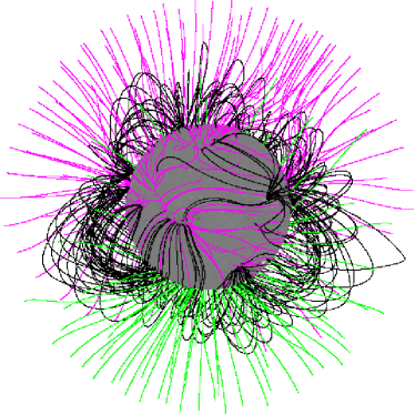
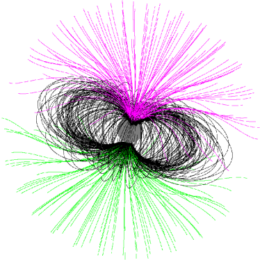
(a)	(b)
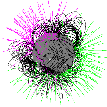
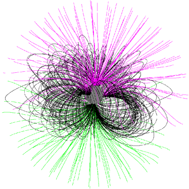
(c)	(d)

Figure 1: The upper (a and b) and lower (c and d) panels represents the PFSS extrapolated magnetic-fields derived from the full disk magnetograms observed on 2011 August 9 (solar minimum) and 2004 July 18 (solar maximum) respectively. The left (a and c) and right (b and d) panels show the extrapolated magnetic-fields from 1.5 – 2.5 $\rm R_{\odot}$ and 5 – 10 $\rm R_{\odot}$ respectively. The gray colored disk at the center is the magnetogram observed at NSO/KP or NSO/SOLIS instruments. The black lines represent the closed field lines. The lines, respectively, in majenta and green indicate the negative and positive polarities of the open magnetic-field lines.

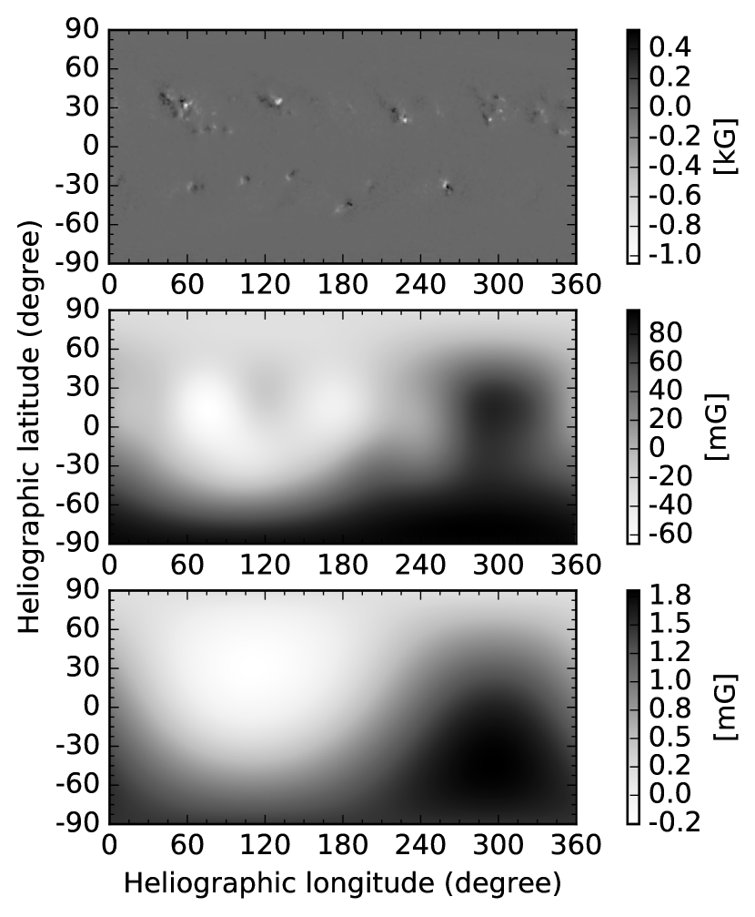
Figure 2: The synoptic magnetogram (upper panel) was observed during the CR2114 using NSO/SOLIS instrument at the wavelength 630.150 nm. The upper panel shows the distribution of observed photospheric magnetic-fields. The middle and lower panels are the extrapolated synoptic magnetograms (of the one in the upper panel) to the source surface 2.5 and 10 $R_{\odot}$ respectively.

3.2 Magnetic-field Measurements

Using the magnetograms observed at photospheric height and the extrapolated magnetograms at $2.5$ and $10~{}R_{\odot}$, we have studied the magnetic-field variations over different range of latitudes. As we are interested in latitudinal variation of the magnetic-field, we find an averaged magnetic-field along longitudes [$\phi_{i,n}$] using

$$\phi_{i,n}={\Sigma_{j=1}^{360}~{}\phi_{i,j,n}\over 360}$$ (1)

where i, j and n are the latitude, longitude, and CR number. After the average, the size of the array reduces to $180\times 1$. Then we measured the averaged magnetic-field [$\phi_{n}$] over selected latitude intervals for a given CR number [n] using

$$\phi_{n}={{\Sigma_{i=k}^{p}\phi_{i,n}}\over{p-k+1}}$$ (2)

where k and p are the row numbers corresponding to the selected latitude bin. Using the Equations 1 and 2, we have measured the magnetic-field over different latitude regions of the Sun and solar corona: i) equatorial or toroidal field (i.e. the fields ranging in the latitude regions from $0^{\circ}$ – $45^{\circ}$); ii) Mid-latitude fields (i.e. the fields ranging in the latitude regions from $46^{\circ}$ - $78^{\circ}$; iii) the fields ranging from $0^{\circ}$ – $78^{\circ}$ (henceforth referred it as Region-A fields); and iv) the polar or polar cap fields (i.e. the fields ranging in the latitude region from $78^{\circ}$ – $90^{\circ}$). The averaged magnetic-fields measured over these latitude regions are shown in Figures 3 and 4.

3.3 Interplanetary Scintillations

If there is an enhancement or depletion of density fluctuations in the solar-wind along the line-of-sight (LOS) to the observed radio source, then there is a corresponding change in scintillation index [m] which defined as

$$m={{\Delta S}\over{\langle S\rangle}},$$ (3)

where $\Delta S$ and $\langle S\rangle$ are the scintillation flux and the mean source flux respectively. The quantity $\Delta S$ is computed from the power spectrum [$P(f)$] of the IPS observation using

$$\Delta S=\int_{0}^{\infty}P(f)df.$$ (4)

The mean source flux ($\langle S\rangle$) can be measured by averaging the difference between onsource and offsource fluxes (Tokumaru et al., 2010). IPS observations of 215 compact extragalactic and radio sources have been carried out on regular basis at 327 MHz. We would note here that all these sources have a finite angular diameter ranging from $\approx 10$ to $500$ milliarcsecond (mas) and observed over different heliocentric distances range from 0.2 to 0.8 AU. It was found that, in general, the quantity m increases with the decreasing heliocentric distance up to a certain distance called turn-over distance and beyond this distance it decreases rapidly with the further decrement in the distance. On the other hand, m decreases if the angular size of the radio source increases. Also, for an ideal point source the scintillating flux will be equal to the mean source flux and thus the scintillation index will be equal to unity at a certain distance (e.g. at 327 MHz, the distance at which $m=1$ corresponds to 0.2 AU) and then decreases with the further increment in the heliocentric distance. Therefore, following Janardhan et al. (2011) and Bisoi et al. (2014), we have normalized the m so that it is independent of the heliocentric distance and a finite source size at that distance. We would make a note that Janardhan et al. (2011) have reported the m after elimination of dependence of the heliocentric distance but not corrected for the finite source sizes. In Bisoi et al. (2014), the reported m is corrected for both dependence of heliocentric distance and the finite source sizes.

For the sake of completeness we have summarized the method of normalization adopted in this article - (1) In order to remove the heliocentric distance dependence of m, each observation of m has to be normalized by that of a point source at that distance. We know that the source 1148-001 has the smaller angular diameter of $\lesssim 10$ mas at 327 MHz and therefore we treat that source to be an ideal point source (Venugopal et al., 1985). (2) Similarly, we have eliminated the dependence of finite source sizes using a least square minimization to determine which of the Marians curves best fits the data for a given source (see Marians, 1975; Bisoi et al., 2014). Assuming the radio source 1148-001 as a point source, the observed values of m of all other sources were multiplied by a factor equal to the difference between the best fit Marians curve for the given source and the best fit Marians curve for 1148-001 at the corresponding heliocentric distance (Bisoi et al., 2014). Therefore, all measurements of m reported in this article were independent of a distance and the sources sizes.

After normalization, we have selected the sources which has at least 400 observations (during 1983-2017) and are uniformly distributed over the entire heliocentric distance (i.e., 0.2-0.8 AU) without a significant data gaps. After such a rigorous filtering, we have left with 27 sources (out of the 215 regularly observed sources) which cover the right ascensions over 24 hours and a wide range of declinations. The blue circles in the Figure 5 indicate the measured annual average of ‘m’ that corresponds to 27 sources separately. The red circles indicate the annual average of m for the all 27 sources in a given year. We would like to make note that in order to avoid unusual error bars (during Solar Cycle 24) because of the significant drop in the m after 2008, we have measured the error bars separately for the years 1983-2008 and 2009-2017. The $1\sigma$ error bars of the annually averaged m values of the observed sources in that year are shown in Figure 5.

  

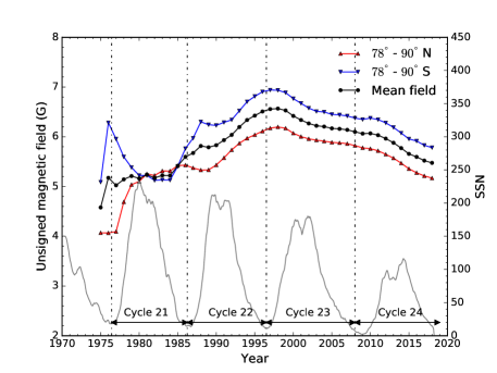
    (a)                                            (b)

  

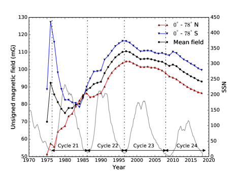
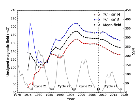
    (c)                                            (d)

  

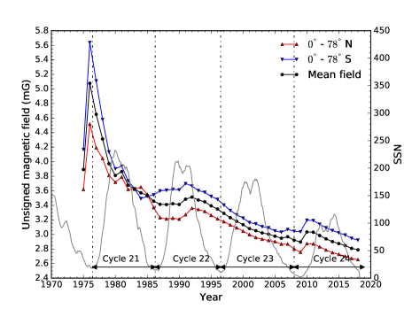
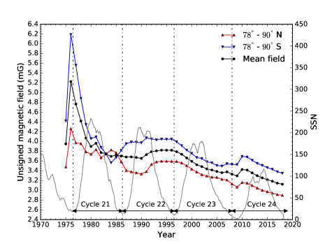
   (e)                                             (f)

Figure 3: Variation of magnetic-field with the solar cycle. The left (a, c, e) and right columns (b, d, f) show the average of Region-A and poloidal fields respectively. In each panel the triangles pointing upward and triangles pointing downward indicate the northern and southern hemispheric fields. The circle in black indicate the average of both northern and southern hemispheric fields. The gray solid line shows the monthly averaged sunspot number (SSN). Panels a and b shows the field on photosphere. The panels c and d show the extrapolated field at $2.5R_{\odot}$. Panels e and f show the extrapolated field at 10 $\rm R_{\odot}$.

  

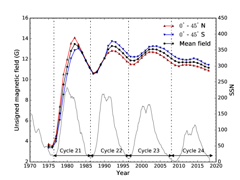
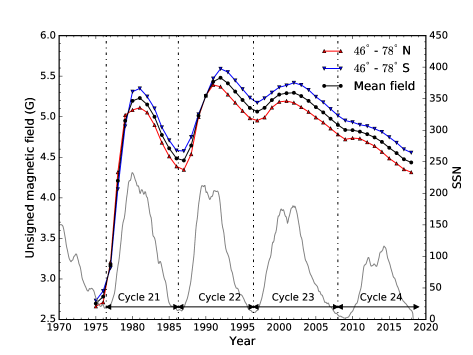
   (a)                                             (b)

  

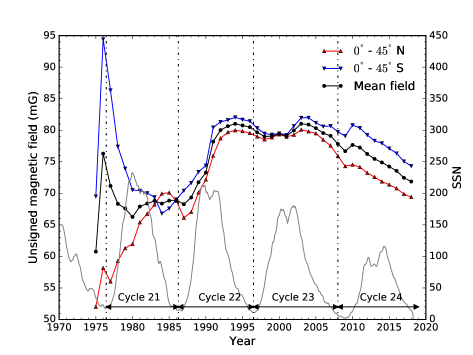
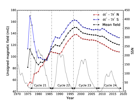
   (c)                                             (d)

  

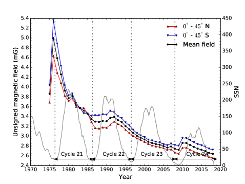
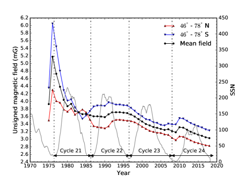
   (e)                                             (f)

Figure 4: Variation of magnetic-field with the solar cycle. The left (a, c, e) and right columns (b, d, f) show the toroidal and mid-latitude fields respectively. In each panel the triangles pointing upward and triangles pointing downward indicate the northern and southern hemispheric fields. The circle in black indicate the average of both northern and southern hemispheric fields. The gray solid line shows the monthly averaged sunspot number (SSN). Panels (a) and (b) shows the field on photosphere. The panels c and d show the extrapolated field at $2.5R_{\odot}$. Panels e and f show the extrapolated field at 10 $\rm R_{\odot}$.

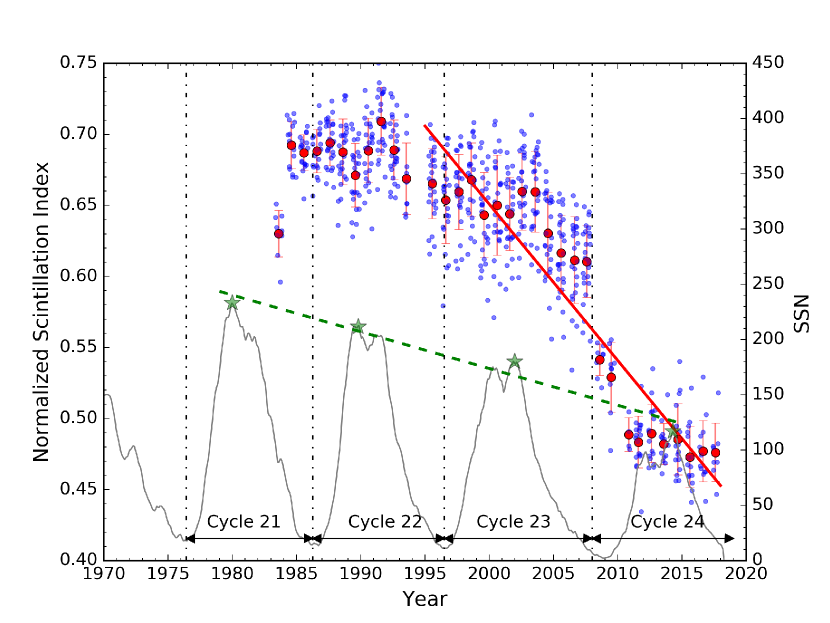
Figure 5: Variation of the normalized scintillation index [$m$] over different years is shown. The blue circles indicate the annually averaged m for different sources. The red circles indicate the annual average of the all sources observed in that year. The fit to the red circles (red solid curve) explicitly shows that the quantity m has been declining since $\approx 1995$. These observations are carried out using the facility at ISEE, Japan at 327 MHz during 1983 – 2017. The gray curve indicate the sunspot number observed during this period. The dashed green line is a fit to observed highest sunspot number during the solar maximum (indicated using green stars) also shows the declining highest sunspot number since Cycle 21.

4 Results and Discussion

Recent reports using angular-broadening observations show that various turbulent parameters (e.g. amplitude of turbulence, density modulation index) correlate well with the solar cycle (Bisoi et al., 2014; Sasikumar Raja et al., 2016, 2017). In this article, we attempted to explore the relationship between the global magnetic-field strength and the turbulence parameters. As previously mentioned, there is no direct method to measure the magnetic-field strength in the corona and hence in order to have some idea of the magnetic-field strength at $10~{}R_{\odot}$ (the distance where, at present, we can probe the solar-wind using IPS observations), we used the PFSS extrapolation technique. We opt for this technique because it is basic and widely used in recent times. This technique is well approximated to the heliocentric distance up 2.5 $\rm R_{\odot}$. However, as the global magnetic-field lines are radial beyond this height, we extrapolated further to 10 $\rm R_{\odot}$. As discussed in Section 3, we inspected the magnetic-field at photosphere, 2.5, and 10 $\rm R_{\odot}$ over different latitudes.

Figures 3 and 4 show the variation of the global magnetic-field with the solar cycle. In Figure 3 panels a, c, e and panels b, d, f show the average of Region-A (latitudes $0^{\circ}-78^{\circ}$) and polar or poloidal fields. Similarly, in Figure 4, panels a, c, e and panels b, d, f show the average of the field in equatorial or toroidal and mid-latitude fields respectively. In both Figures 3 and 4, in each panel the triangles pointing upward and triangles pointing downward indicate the northern and southern hemispheric fields. The circles in black indicate the mean field of both northern and southern hemispheric fields (i.e. average of the points shown in triangles both upward and downward). In each panel, for reference, the smoothed, monthly average, sunspot number (SSN) is shown as a gray solid line (http://www.sidc.be/silso/DATA/SN_ms_tot_V2.0.txt). In both Figures 3 and 4, panels a and b show the magnetic-field at photospheric heights. Panels c and d show the extrapolated field at $2.5~{}\rm R_{\odot}$ and panels e and f show the extrapolated field at 10 $\rm R_{\odot}$.

From Figures 3 and 4, it is clear that magnetic-field has been declining since mid 1990s. Various observationally derived parameters are tabulated in Table 1. The latitude range over which the magnetic-field is averaged is shown in column 2. The year from when the beginning of significant decline of the field is shown in column 3 and the corresponding field in column 4. Similarly for the year 2018 the measured magnetic-field is shown in column 6. We measured the decrement in magnetic-field (in percent) from mid-1990s to 2018 (at photosphere, 2.5, and 10 $\rm R_{\odot}$) and tabulated it in column 7. We found that magnetic-field over different range of latitudes and heliocentric distances are declined by $11-22.2\,\%$. These results are very significant support for the conclusion that not only were the polar fields declining since mid-1990, as previously reported (Janardhan et al., 2011, 2015) but the overall (global) coronal magnetic-field is also declining. We found that, in phase with the global magnetic-fields, the quantity m also declined by $23.6\,\%$ from the mid 1990s to 2017. These results show that the global magnetic-field is controlling the turbulence characteristics in the solar corona and solar-wind.

Another notable observation is that we see an oscillation of magnetic-field at the photospheric height in correlation with the sunspot number (see panels a and b of Figures 3 and 4). We examined such variation (from solar maximum to minimum) of the mean magnetic-field (see Figures 3 and 4) in each solar cycle (from Solar Cycle 22 to 24) and found that it varied by $\approx 5-10\,\%$ . We found that such oscillating behavior (due to sunspots) disappears in the solar corona and solar-wind (see panels c, d, e and f of Figures 3 and 4) and shows a clear monotonic decline of the coronal magnetic-field (by $11-22.2\,\%$).

We also would like to make a note that in Figure 5, the quantity m (the red circles) shows a negative jumps near the solar maximum which can be interpreted as follows - Sasikumar Raja et al. (2016) have reported that the density modulation index (i.e. $\epsilon_{N}=\Delta N/N$; where $\Delta N$ and N are the density fluctuations and the background density respectively) positively correlates with the solar-wind speed. For the sake of completeness we provide the explanation given by them as follows. It was reported that the $\epsilon_{N}$ positively correlates with the temperature of solar-wind protons (Celnikier et al., 1987). Also, it was found that at 1 AU, the proton temperature positively correlates with solar-wind speed (Lopez & Freeman, 1986). Taken together, authors have concluded that $\epsilon_{N}$ should be larger in the fast solar-wind and lower in the slow solar-wind. We also know that during the solar minimum the global magnetic-field is dipolar and therefore, during solar minimum higher latitudes drive the fast solar-wind (because of the dominant polar coronal holes) and drive the slow solar-wind near the low latitudes. On the other hand, during solar maximum, the global magnetic-field is multi-polar and thus drives the slow solar-wind in all helio-latitudes as the polar coronal holes are not prevalent (McComas et al., 2000; Asai et al., 1998). Therefore, during solar maximum the slow solar-wind suggests the lower density modulation index which in-turn is proportional to the quantity m (see Bisoi et al., 2014) and hence the negative jumps during solar maximum is consistent with the earlier reports.

	Latitude	Epoch - I		Epoch - II		Decrement
No.	range	Year	Mean field [G]	Year	Mean field [G]	in [$\%$]
(1)	(2)	(3)	(4)	(5)	(6)	(7)
Photosphere
1	$0^{\circ}-78^{\circ}$	1992	9.98	2018	8.32	16.6
2	$78^{\circ}-90^{\circ}$	1997	6.56	2018	5.48	16.5
3	$0^{\circ}-45^{\circ}$	1992	13.28	2018	11.17	15.9
4	$45^{\circ}-78^{\circ}$	1992	5.48	2018	4.44	19.1
$2.5~{}\rm R_{\odot}$
1	$0^{\circ}-78^{\circ}$	1996	0.11	2018	0.09	15.4
2	$78^{\circ}-90^{\circ}$	1997	0.19	2018	0.15	20.6
3	$0^{\circ}-45^{\circ}$	1994	0.08	2018	0.07	11.3
4	$45^{\circ}-78^{\circ}$	1997	0.15	2018	0.12	19.8
$10~{}\rm R_{\odot}$
1	$0^{\circ}-78^{\circ}$	1992	$3.51\times 10^{-3}$	2018	$2.79\times 10^{-3}$	20.6
2	$78^{\circ}-90^{\circ}$	1994	$3.82\times 10^{-3}$	2018	$3.12\times 10^{-3}$	18.2
3	$0^{\circ}-45^{\circ}$	1992	$3.39\times 10^{-3}$	2018	$2.64\times 10^{-3}$	22.2
4	$45^{\circ}-78^{\circ}$	1993	$3.71\times 10^{-3}$	2018	$3.03\times 10^{-3}$	18.4

Table 1: The averaged magnetic-field strength at different epochs (mid 1990s and 2018) over different latitudes are shown. The decrement of the magnetic-field (in $\%$) over these epochs are shown in column 7. The measurements are tabulated for photospheric height, $2.5$, and $10~{}\rm R_{\odot}$.

5 Summary and Conclusion

Using the synoptic magnetogram data observed using NSO/KP and NSO/SOLIS instruments during the period from 1975 to April 2018, we inspected the average magnetic-fields (at the photosphere) over different latitude ranges in both northern and southern hemispheres. We have noticed that not only the polar magnetic-field, but the equatorial, mid-latitude, and fields in Region A are also declining, since the mid-1990s (see Figures 3, 4; and Table 1). Further, we have inspected the magnetograms extrapolated (using the PFSS method) to the heliocentric distances to 2.5 and 10 $\rm R_{\odot}$ and they also show the same trend. We found that, during the period from the mid-1990s to April 2018, the magnetic-field over different latitudes (at photosphere and inner solar-wind) declined by $11.3-22.2\,\%$. Using the data observed from ISEE, Japan, we inspected the normalized scintillation index [$m$] during 1983 – 2017. We found that the quantity m has decreased by $23.6\,\%$ since the mid-1990s. From Figure 5, it is clear that the peak sunspot number from Solar Cycle 21 (in the year 1980) to Solar Cycle 24 (in year 2014) has declined by $\approx 50\,\%$. Therefore, these results show a strong relationship between the global magnetic-fields and the various turbulence properties in the solar-wind. Also, we found that magnetic-field at relatively low heights shows a monotonic decrease (by $15.9-19.1\,\%$; see Table 1) as well as a variation of the magnetic-field (due to sunspots) over each solar cycle by $5-10\,\%$. Such oscillating behavior disappears in the inner solar-wind (i.e. at 2.5 and $10~{}\rm R_{\odot}$) and a clear monotonic decline of the magnetic-field is seen (by $11.3-22.2\,\%$). In this article we show that the global coronal magnetic-field of the Sun (and not just the polar fields) has monotonically decreased since (approximately) 1995. These results are significant, as many authors are predicting that we are tending towards the another “Maunder”-like minimum (Janardhan et al., 2011, 2015, 2018; Pesnell & Schatten, 2018). It would be interesting to further examine the relationship between the global (large-scale) magnetic-field and the properties of density turbulence (which are measured by IPS). For example, the way magnetic-field and the turbulence properties in the solar-wind (i.e. amplitude of the turbulence, density, velocity and magnetic-field fluctuations, dissipation scales, and heating rates etc.) are related (Bisoi et al., 2014; Sasikumar Raja et al., 2016, 2017, 2019). The recently launched Parker Solar Probe may provide valuable insights in understanding the relationship between the magnetic-field and the turbulent parameters (Fox et al., 2016).

References

- Altschuler & Newkirk (1969) Altschuler, M. D., & Newkirk, G. 1969, Sol. Phys., 9, 131, doi: 10.1007/BF00145734
- Ananthakrishnan et al. (1980) Ananthakrishnan, S., Coles, W. A., & Kaufman, J. J. 1980, J. Geophys. Res., 85, 6025, doi: 10.1029/JA085iA11p06025
- Arnaud & Newkirk (1987) Arnaud, J., & Newkirk, Jr., G. 1987, A&A, 178, 263
- Asai et al. (1998) Asai, K., Kojima, M., Tokumaru, M., et al. 1998, J. Geophys. Res., 103, 1991, doi: 10.1029/97JA02750
- Bird (1981) Bird, M. K. 1981, in Solar Wind 4, ed. H. Rosenbauer, 78
- Bird (1982) Bird, M. K. 1982, Space Sci. Rev., 33, 99, doi: 10.1007/BF00213250
- Bisoi et al. (2014) Bisoi, S. K., Janardhan, P., Ingale, M., et al. 2014, ApJ, 795, 69, doi: 10.1088/0004-637X/795/1/69
- Celnikier et al. (1987) Celnikier, L. M., Muschietti, L., & Goldman, M. V. 1987, A&A, 181, 138
- Clette et al. (2015) Clette, F., Svalgaard, L., Vaquero, J. M., & Cliver, E. W. 2015, Revisiting the Sunspot Number, ed. A. Balogh, H. Hudson, K. Petrovay, & R. von Steiger, 35
- Fox et al. (2016) Fox, N. J., Velli, M. C., Bale, S. D., et al. 2016, Space Science Reviews, 204, 7, doi: 10.1007/s11214-015-0211-6
- Freeland & Handy (1998) Freeland, S. L., & Handy, B. N. 1998, Sol. Phys., 182, 497, doi: 10.1023/A:1005038224881
- Hale (1908) Hale, G. E. 1908, ApJ, 28, 315, doi: 10.1086/141602
- Harvey (1969) Harvey, J. W. 1969, PhD thesis, Univ. Colorado, Boulder.
- Hewish et al. (1964) Hewish, A., Scott, P. F., & Wills, D. 1964, Nature, 203, 1214, doi: 10.1038/2031214a0
- Hoeksema (1984) Hoeksema, J. T. 1984, PhD thesis, Stanford Univ., CA.
- Janardhan & Alurkar (1993) Janardhan, P., & Alurkar, S. K. 1993, A&A, 269, 119
- Janardhan et al. (1996) Janardhan, P., Balasubramanian, V., Ananthakrishnan, S., et al. 1996, Sol. Phys., 166, 379, doi: 10.1007/BF00149405
- Janardhan et al. (2011) Janardhan, P., Bisoi, S. K., Ananthakrishnan, S., Tokumaru, M., & Fujiki, K. 2011, Geophys. Res. Lett., 38, L20108, doi: 10.1029/2011GL049227
- Janardhan et al. (2015) Janardhan, P., Bisoi, S. K., Ananthakrishnan, S., et al. 2015, J. Geophys. Res., 120, 5306, doi: 10.1002/2015JA021123
- Janardhan et al. (2010) Janardhan, P., Bisoi, S. K., & Gosain, S. 2010, Sol. Phys., 267, 267, doi: 10.1007/s11207-010-9653-x
- Janardhan et al. (2018) Janardhan, P., Fujiki, K., Ingale, M., Bisoi, S. K., & Rout, D. 2018, A&A, 618, A148, doi: 10.1051/0004-6361/201832981
- Kojima & Kakinuma (1990) Kojima, M., & Kakinuma, T. 1990, Space Sci. Rev., 53, 173, doi: 10.1007/BF00212754
- Lin et al. (2000) Lin, H., Penn, M. J., & Tomczyk, S. 2000, ApJ, 541, L83, doi: 10.1086/312900
- Lopez & Freeman (1986) Lopez, R. E., & Freeman, J. W. 1986, J. Geophys. Res., 91, 1701, doi: 10.1029/JA091iA02p01701
- Mackay & van Ballegooijen (2006) Mackay, D. H., & van Ballegooijen, A. A. 2006, ApJ, 641, 577, doi: 10.1086/500425
- Manoharan (2010) Manoharan, P. K. 2010, Sol. Phys., 265, 137, doi: 10.1007/s11207-010-9593-5
- Marians (1975) Marians, M. 1975, Radio Science, 10, 115, doi: 10.1029/RS010i001p00115
- McComas et al. (2000) McComas, D. J., Barraclough, B. L., Funsten, H. O., et al. 2000, J. Geophys. Res., 105, 10419, doi: 10.1029/1999JA000383
- Mickey (1973) Mickey, D. L. 1973, ApJ, 181, L19, doi: 10.1086/181175
- Pesnell & Schatten (2018) Pesnell, W. D., & Schatten, K. H. 2018, Sol. Phys., 293, 112, doi: 10.1007/s11207-018-1330-5
- Querfeld & Smartt (1984) Querfeld, C. W., & Smartt, R. N. 1984, Sol. Phys., 91, 299, doi: 10.1007/BF00146301
- Ramesh et al. (2010) Ramesh, R., Kathiravan, C., & Sastry, C. V. 2010, ApJ, 711, 1029, doi: 10.1088/0004-637X/711/2/1029
- Sasikumar Raja et al. (2016) Sasikumar Raja, K., Ingale, M., Ramesh, R., et al. 2016, J. Geophys. Res., 121, 11, doi: 10.1002/2016JA023254
- Sasikumar Raja & Ramesh (2013) Sasikumar Raja, K., & Ramesh, R. 2013, ApJ, 775, 38, doi: 10.1088/0004-637X/775/1/38
- Sasikumar Raja et al. (2014) Sasikumar Raja, K., Ramesh, R., Hariharan, K., Kathiravan, C., & Wang, T. J. 2014, ApJ, 796, 56, doi: 10.1088/0004-637X/796/1/56
- Sasikumar Raja et al. (2019) Sasikumar Raja, K., Subramanian, P., Ingale, M., & Ramesh, R. 2019, ApJ, 872, 77, doi: 10.3847/1538-4357/aafd33
- Sasikumar Raja et al. (2017) Sasikumar Raja, K., Subramanian, P., Ramesh, R., Vourlidas, A., & Ingale, M. 2017, ApJ, 850, 129, doi: 10.3847/1538-4357/aa94cd
- Sastry (2009) Sastry, C. V. 2009, ApJ, 697, 1934, doi: 10.1088/0004-637X/697/2/1934
- Schatten et al. (1969a) Schatten, K. H., Wilcox, J. M., & Ness, N. F. 1969a, Sol. Phys., 6, 442, doi: 10.1007/BF00146478
- Schatten et al. (1969b) —. 1969b, Sol. Phys., 6, 442, doi: 10.1007/BF00146478
- Schrijver & De Rosa (2003) Schrijver, C. J., & De Rosa, M. L. 2003, Sol. Phys., 212, 165, doi: 10.1023/A:1022908504100
- Schrijver & Title (2003) Schrijver, C. J., & Title, A. M. 2003, ApJ, 597, L165, doi: 10.1086/379870
- Stelzried et al. (1970) Stelzried, C. T., Levy, G. S., Sato, T., et al. 1970, Sol. Phys., 14, 440, doi: 10.1007/BF00221330
- Tokumaru et al. (2010) Tokumaru, M., Kojima, M., & Fujiki, K. 2010, J. Geophys. Res., 115, A04102, doi: 10.1029/2009JA014628
- van Ballegooijen et al. (2000) van Ballegooijen, A. A., Priest, E. R., & Mackay, D. H. 2000, ApJ, 539, 983, doi: 10.1086/309265
- Venugopal et al. (1985) Venugopal, V. R., Ananthakrishnan, S., Swarup, G., Pynzar, A. V., & Udaltsov, V. A. 1985, MNRAS, 215, 685, doi: 10.1093/mnras/215.4.685
- Wang & Sheeley (1992) Wang, Y.-M., & Sheeley, Jr., N. R. 1992, ApJ, 392, 310, doi: 10.1086/171430
- Zhao & Hoeksema (1995) Zhao, X., & Hoeksema, J. T. 1995, J. Geophys. Res., 100, 19, doi: 10.1029/94JA02266