Disjunct Support Spike and Slab Priors for Variable Selection in Regression under Quasi-sparseness

Abstract

Sparseness of the regression coefficient vector is often a desirable property, since, among other benefits, sparseness improves interpretability. In practice, many true regression coefficients might be negligibly small, but non-zero, which we refer to as quasi-sparseness. Spike-and-slab priors as introduced in (Chipman et al., 2001) can be tuned to ignore very small regression coefficients, and, as a consequence provide a trade-off between prediction accuracy and interpretability. However, spike-and-slab priors with full support lead to inconsistent Bayes factors, in the sense that the Bayes factors of any two models are bounded in probability. This is clearly an undesirable property for Bayesian hypotheses testing, where we wish that increasing sample sizes lead to increasing Bayes factors favoring the true model. The moment matching priors as in (Johnson and Rossell, 2012) can resolve this issue, but are unsuitable for the quasi-sparse setting due to their full support outside the exact value 0. As a remedy, we suggest disjunct support spike and slab priors, for which we prove consistent Bayes factors in the quasi-sparse setting, and show experimentally fast growing Bayes factors favoring the true model. Several experiments on simulated and real data confirm the usefulness of our proposed method to identify models with high effect size, while leading to better control over false positives than hard-thresholding.

1 Introduction

Sparseness of the regression coefficient vector is often a desirable property, since it (1) helps to improve interpretability, and (2) reduces the cost of prediction. In particular, we are interested here in the setting when the sparsity assumptions regarding exact zero regression coefficients are violated, and many regression coefficients might be non-zero but have negligible magnitude. This is also sometimes referred to as quasi-sparseness (Datta and Dunson, 2016). In such situations, we may have to trade in a small reduction in prediction accuracy for an increase in sparseness.

Spike-and-slab priors, as proposed by (Chipman et al., 2001), can potentially handle such a trade-off between prediction accuracy and sparseness. Though, manual setting of these priors is difficult, since they are either too restrictive, or depend on the unknown noise variance of the response variable. The limitations of these previous approaches are basically due to the desire for conjugate priors which results in closed-form solutions for the marginal likelihood.

Here, in this work, we propose a hierarchical spike-and-slab prior for the linear regression model that allows the user to explicitly specify the minimal magnitude $\delta$ of the regression coefficients that is considered practically significant. The proposed model decouples the response noise prior variance from the regression coefficients’ prior variance, and thus making the threshold parameter $\delta$ more meaningful than previous work (Chipman et al., 2001). For example, $\delta$ can be set such that the Mean-Squared Error (MSE) of the prediction is only little influenced by ignoring covariates with coefficients’ magnitude smaller than $\delta$.

Our proposed method also resolves another subtle issue with the spike-and-slab priors from (Chipman et al., 2001), namely inconsistent Bayes factors (BF). Due to the fact that the spike-and-slab priors of (Chipman et al., 2001) (and related work like (Ishwaran et al., 2005)) have full support, the Bayes factors of any two models is bounded in probability, for which we give a formal proof in Section 4. This is an undesirable property for Bayesian hypothesis testing, since we would like that the BF between the true and the wrong model grows with increasing sample size. In order to resolve this issue, our proposed method uses disjunct support priors, which allows us to guarantee consistent Bayes factors that grow exponentially fast favoring the true model.

Though our choice of the priors allows us to prove consistent Bayes factors, our choice complicates the calculation of the marginal likelihood. As a solution, we propose to estimate all Bayes factors by introducing a latent variable indicator vector $\mathbf{z}$, with an efficient Gibbs sampler to sample from its posterior distribution.

We note that (Johnson and Rossell, 2012) also proposed the use of disjunct support priors for variable selection in linear regression. However, the difference in support of their spike and slab priors is only at $\{0\}$, which makes them unsuitable for the quasi-sparse setting.

The rest of this article is organized as follows. In the next section, we summarize the properties of spike-and-slab priors from previous work. In Section 3, we introduce our model for variable selection based on disjunct support spike-and-slab priors. In Section 4, we prove that the disjunct support priors of our proposed method allows us to guarantee consistent Bayes factors, and compare this to the asymptotic results for other spike-and-slab priors. In Section 5, we explain our MCMC sampling strategy for estimating model probabilities. Since the elicitation of $\delta$ can be difficult, we discuss in Section 6 a strategy for determining $\delta$ by estimating the increase in mean squared error (MSE) for prediction. We evaluate our proposed method on several simulated data sets in Section 7, and real data sets in Section 8. Finally, we summarize our findings in Section 9.

2 Related work

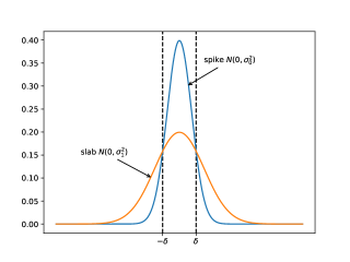
Figure 1: Example of spike and slab prior as proposed in (Chipman et al., 2001): both spike and slab priors are normal distributions but with different variances $\sigma_{0}^{2}$ and $\sigma_{1}^{2}$. The variances $\sigma_{0}^{2}$ and $\sigma_{1}^{2}$ are specified such that the probability density of the spike prior dominates the one of the slab prior in the interval $[-\delta,\delta]$, otherwise the slab prior dominates.

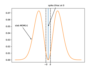
Figure 2: Example of spike and slab prior as proposed in (Johnson and Rossell, 2012): spike distribution is a Dirac measure at point 0, and slab distribution is the moment matching prior with shape parameter $\tau$. Parameter $\tau$ is specified such that the probability mass of $[-\delta,\delta]$ is 0.01 as suggested in (Johnson and Rossell, 2010).

A natural way to handle noise for variable selection are the spike-and-slab priors as proposed in (Chipman et al., 2001). The basic idea is to model the coefficients of the relevant and non-relevant variables by a normal distribution with variances $\sigma_{1}^{2}$ and $\sigma_{0}^{2}$, respectively, and $\sigma_{1}^{2}\gg\sigma_{0}^{2}$. An example is shown in Figure 1.

The variance parameters $\sigma_{1}^{2}$ and $\sigma_{0}^{2}$ must be set manually. A difficulty of spike-and-slab priors is the correct setting of these parameters, and therefore Ishwaran et al. (2005) proposed to place hyper-priors over these parameters in such a way that the resulting marginal prior $p(\boldsymbol{\beta})$ is little sensitive to the hyper-parameter choice. However, their prior choice does not allow for a closed-form marginal likelihood. Furthermore, their prior choice is only suitable for the situation where there is no noise, i.e. a variable $j$ is considered to be relevant if and only if the true coefficient $\beta_{j}$ is not zero.

In contrast, the spike and slab priors proposed in (Chipman et al., 2001) allow to specify practical significance (what we call here “relevance") by setting $\sigma_{1}^{2}$ to some large enough value (for example 100) and then set $\sigma_{0}^{2}$ such that the intersection points of the two priors occur at a pre-specified value $\delta$ (and $-\delta$), see Figure 1. However, their method has some drawbacks:

• Their conjugate prior formulation is sensitive to the prior for the response variance, whereas their non-conjugate formulation is not sensitive to the response variance, but has no closed-form solution anymore.

• For any $\delta>0$, the Bayes factors are not consistent in the following sense. Let $S$ be the true set of relevant variables and $S^{\prime}$ any other set, then we have

  $$\frac{p(\mathbf{y}_{n}|X_{n},S)}{p(\mathbf{y}_{n}|X_{n},S^{\prime})}\stackrel{{\scriptstyle P}}{{\rightarrow}}O_{p}(1)\,,$$

  where $\mathbf{y}_{n}:=(y_{1},\ldots y_{n})$ and $X_{n}:=(\mathbf{x}_{1},\ldots,\mathbf{x}_{n})$, are the observed responses and covariates of $n$ samples. This is due to the fact that the model dimension of spike-and-slab priors is the same for model $S$ and $S^{\prime}$. As a consequence, the influence of the prior can be ignored, in the sense that the influence of the prior is asymptotically the same for model $S$ and $S^{\prime}$. For both models, the posterior distribution of $\boldsymbol{\beta}$ will concentrate around the true regression coefficient vector, and thus, the marginal likelihood cannot be distinguished any more. A formal proof will be given in Section 4.

• It might be difficult to specify $\delta$ a-priori.

Another method to handle noise on regression coefficients is to use nonlocal priors, as proposed in (Johnson and Rossell, 2012; Rossell and Telesca, 2017), for the slab which places very small probability mass on the interval $[-\delta,\delta]\setminus\{0\}$ and its density is exact zero on $\{0\}$. For the spike distribution they suggest to use the Dirac measure at 0. The resulting spike and slab prior is illustrated in Figure 2. Therefore, their proposed spike and slab priors also have disjunct support, and as such enjoy exponentially fast growing Bayes factors (Johnson and Rossell, 2010). However, since the spike distribution has zero mass on $[-\delta,\delta]\setminus\{0\}$, it is unsuitable for the quasi-sparse setting. We analyze the asymptotic behavior of nonlocal priors in the quasi-sparse setting in Theorem 3, in Section 4, and the finite sample behavior in our experiments, in Section 7.1. Interestingly, the nonlocal prior can be considered as a mixture of a truncated normal distribution with threshold $\delta$ and a uniform prior for $\delta$ (Rossell and Telesca, 2017). The prior on $\delta$ is uniform prior on an interval around $0$, where the length of the interval is controlled by the critical parameter $\tau$. Therefore, the difficulty of specifying $\delta$ is shifted to the problem of specifying $\tau$. Recently, Cao et al. (2018) proposed to place a prior on $\tau$, instead of specifying a fixed value. However, their implementation relies on a Laplace approximation which does not enjoy any theoretic guarantees.

Finally, we note that recently Miller and Dunson (2018) proposed a new framework, named $c$-posteriors, which can be applied to handle slight violations from the sparsity assumption. However, their method introduces a hyper-parameter $c$ which might be difficult to interpret. Furthermore, their approach does not allow for the calculation of Bayes factors anymore.

3 Proposed method

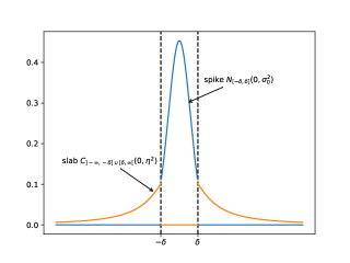
Figure 3: Illustration of the proposed spike and slab prior. $C_{]-\infty,-\delta]\cup[\delta,\infty[}(0,\eta^{2})$ denotes the Cauchy distribution with mean 0 and scale $\eta^{2}$.

Let $S$ be the indices of the selected covariates (i.e. the covariate that are considered to be relevant), and $\mathcal{C}:=\{1,\ldots,d\}\setminus\mathcal{S}$ the set of irrelevant covariates. Furthermore, let $s:=|\mathcal{S}|$ be the number of selected covariates. We consider the following linear model for $y\in\mathbb{R}$ regressed on $\mathbf{x}\in\mathbb{R}^{d}$:

$$y=\mathbf{x}^{T}\boldsymbol{\beta}+\epsilon\,,$$

where

$$\left.\begin{aligned} &\epsilon\sim N(0,\sigma_{r}^{2})\,,\\ &\sigma_{r}^{2}\sim\text{Inv-}\chi^{2}(\nu_{r},\eta_{r}^{2})\,,\end{aligned}\quad\qquad\qquad\qquad\qquad\right\}\text{Prior for noise $\epsilon$}$$

$$\left.\begin{aligned} &s\sim\text{Multinomial}(p,\pi_{\text{rel}})\,,\\ &\pi_{\text{rel}}\sim\text{Beta}(1,1)\,,\\ \end{aligned}\quad\qquad\qquad\qquad\right\}\text{Prior for number of relevant covariates $s$}$$

$$\left.\begin{aligned} &\sigma_{1}^{2}\sim\text{Inv-}\chi^{2}(\nu_{1},\eta_{1}^{2})\,,\\ &\text{for $j\in\{1,\ldots,d\}$:}\\ &\quad\text{if $j\in S$, then}\\ &\quad\quad\beta_{j}\sim N_{]-\infty,-\delta]\cup[\delta,\infty[}(0,\sigma_{1}^{2})\\ &\quad\text{else}\\ &\quad\quad\beta_{j}\sim N_{[-\delta,\delta]}(0,\sigma_{0}^{2})\,.\\ \end{aligned}\qquad\quad\quad\;\right\}\text{Prior for regression coefficients $\boldsymbol{\beta}$}$$

$\nu_{r},\eta_{r}^{2}$ are set such that $\text{Inv-}\chi^{2}(\nu_{r},\eta_{r}^{2})$ is a weakly informative prior. $\text{Inv-}\chi^{2}$ denotes the scaled inverse chi-square distribution (see details below), where $\nu_{r}$ can be interpreted as the number of a-priori observations. For our experiments, we set $\nu_{r}$ and the prior variance $\sigma_{r}^{2}$ to 1.

$N_{[-\delta,\delta]}$ and $N_{]-\infty,-\delta]\cup[\delta,\infty[}$ denote the truncated normal distribution with support $[-\delta,\delta]$ and $]-\infty,-\delta]\cup[\delta,\infty[$ for the spike and slab prior, respectively. The specification of $\sigma_{0}^{2}$, and $\sigma_{1}^{2}$ determines the shape of the spike and slab prior, respectively. For the slab prior, in order to allow for possibly large values of $\beta_{j}$, we place a diffuse hyper-prior on $\sigma_{1}^{2}$. In particular, we set $\nu_{1}=1$, and $\eta_{1}^{2}=100$ which corresponds to a truncated Cauchy distribution with mean zero and scale $\eta_{1}^{2}$ for $p(\beta_{j}|j\in S,\nu_{1},\eta_{1}^{2},\delta)$.

At the boundary $\beta_{j}=\delta$ (and, due to symmetry $\beta_{j}=-\delta$) we want to be indifferent about whether $\beta_{j}$ was sampled from the spike or slab prior. Therefore, we set $\sigma_{0}^{2}$ such that

$$p(\beta_{j}=\delta|j\in S,\nu_{1},\eta_{1}^{2},\delta)=p(\beta_{j}=\delta|j\notin S,\sigma_{0}^{2},\delta)\,.$$ (1)

The left hand side of Equation (1) does not have a closed-form solution. However, note that

$$p(\beta_{j}=\delta|j\in S,\nu_{1},\eta_{1}^{2},\delta)=\int N_{]-\infty,-\delta]\cup[\delta,\infty[}(\beta_{j}=\delta|0,\sigma_{1}^{2})\cdot\text{Inv-}\chi^{2}(\sigma_{1}^{2}|\nu_{1},\eta_{1}^{2})d\sigma_{1}^{2}\,,$$

which we solve using numerical integration. Our proposed spike and slab prior is illustrated in Figure 3.

Therefore, the remaining critical hyper-parameter is only the specification of the threshold parameter $\delta$. In Section 6, we discuss the specification of $\delta$.

Note that the prior on the number of relevant variables $s$ ensures multiplicity control and has been extensively studied in (Scott et al., 2010; Scott and Berger, 2006). The probability of a variable being relevant $\pi_{\text{rel}}$ can be integrated out leading to

$$p(s)=\frac{1}{d+1}\left(\begin{array}[]{c}d\\ s\end{array}\right)^{-1}\,.$$

Note that the scaled inverse chi-square distribution is defined as follows (see e.g. Gelman et al. (2013)):

$$\text{Inv-}\chi^{2}(\sigma^{2}|\nu,\eta^{2}) =(\eta^{2})^{\nu/2}\frac{(\nu/2)^{\nu/2}}{\Gamma(\nu/2)}(\sigma^{2})^{-(\frac{\nu}{2}+1)}e^{-\frac{1}{2\sigma^{2}}\nu\eta^{2}}\,.$$

Therefore, the joint probability density function is given by:

$$p(\boldsymbol{\beta},\sigma_{r}^{2},\sigma_{1}^{2},\mathbf{y},S,|X) =p(s)\cdot(2\pi)^{-\frac{n}{2}}\cdot(\sigma_{r}^{2})^{-\frac{n}{2}}e^{-\frac{1}{2\sigma_{r}^{2}}||\mathbf{y}-X\boldsymbol{\beta}||_{2}^{2}}$$

$$\quad\cdot(\eta_{r}^{2})^{\nu_{r}/2}\frac{(\nu_{r}/2)^{\nu_{r}/2}}{\Gamma(\nu_{r}/2)}\cdot(\sigma_{r}^{2})^{-(\frac{\nu_{r}}{2}+1)}e^{-\frac{1}{2\sigma_{r}^{2}}\nu_{r}\eta_{r}^{2}}$$

$$\quad\cdot(\eta_{1}^{2})^{\nu_{1}/2}\frac{(\nu_{1}/2)^{\nu_{1}/2}}{\Gamma(\nu_{1}/2)}\cdot(\sigma_{1}^{2})^{-(\frac{\nu_{1}}{2}+1)}e^{-\frac{1}{2\sigma_{1}^{2}}\nu_{1}\eta_{1}^{2}}$$

$$\quad\cdot\Big{(}\prod_{j\in\mathcal{C}}\mathbbm{1}_{\mathcal{N}}(\beta_{j})\cdot\frac{1}{\iota(\mathcal{N},\sigma_{0}^{2})}\cdot e^{-\frac{1}{2\sigma_{0}^{2}}\beta_{j}^{2}}\Big{)}$$

$$\quad\cdot\Big{(}\prod_{j\in\mathcal{S}}\mathbbm{1}_{\mathcal{R}}(\beta_{j})\cdot\frac{1}{\iota(\mathcal{R},\sigma_{1}^{2})}e^{-\frac{1}{2\sigma_{1}^{2}}\beta_{j}^{2}}\Big{)}$$

$$=C_{0}\cdot p(s)\cdot(\sigma_{r}^{2})^{-\frac{n}{2}}e^{-\frac{1}{2\sigma_{r}^{2}}||\mathbf{y}-X\boldsymbol{\beta}||_{2}^{2}}$$

$$\quad\cdot(\sigma_{r}^{2})^{-(\frac{\nu_{r}}{2}+1)}e^{-\frac{1}{2\sigma_{r}^{2}}\nu_{r}\eta_{r}^{2}}$$

$$\quad\cdot(\sigma_{1}^{2})^{-(\frac{\nu_{1}}{2}+1)}e^{-\frac{1}{2\sigma_{1}^{2}}\nu_{1}\eta_{1}^{2}}$$

$$\quad\cdot\Big{(}\prod_{j\in\mathcal{C}}\mathbbm{1}_{\mathcal{N}}(\beta_{j})\cdot\frac{1}{\iota(\mathcal{N},\sigma_{0}^{2})}\cdot e^{-\frac{1}{2\sigma_{0}^{2}}\beta_{j}^{2}}\Big{)}$$

$$\quad\cdot\Big{(}\prod_{j\in\mathcal{S}}\mathbbm{1}_{\mathcal{R}}(\beta_{j})\cdot\frac{1}{\iota(\mathcal{R},\sigma_{1}^{2})}e^{-\frac{1}{2\sigma_{1}^{2}}\beta_{j}^{2}}\Big{)}\,,$$

where we defined $\mathcal{N}:=[-\delta,\delta]$, and $\mathcal{R}:=]-\infty,-\delta]\cup[\delta,\infty[$, and

$$\iota(\mathcal{A},\sigma^{2}):=\int\mathbbm{1}_{\mathcal{A}}(x)e^{-\frac{1}{2\sigma^{2}}x^{2}}dx$$

and

$$C_{0} :=(2\pi)^{-\frac{n}{2}}\cdot(\eta_{r}^{2})^{\nu_{r}/2}\frac{(\nu_{r}/2)^{\nu_{r}/2}}{\Gamma(\nu_{r}/2)}\cdot(\eta_{1}^{2})^{\nu_{1}/2}\frac{(\nu_{1}/2)^{\nu_{1}/2}}{\Gamma(\nu_{1}/2)}\,.$$

4 Asymptotic Bayes factors

In this section, we formally prove the asymptotic behavior of the Bayes factors between the true model and any other model, first for our proposed method, in Theorem 1, and then for previously proposed spike and slab priors, in Theorem 2 and Theorem 3.

In the following, we define the true set of relevant variables $S$ as

$$S:=\Big{\{}j\in\{1,\ldots,d\}\Big{|}\;|\;\beta_{j,t}|>\delta\Big{\}}\,.$$ (2)

Furthermore, we denote convergence in probability by $\stackrel{{\scriptstyle P}}{{\rightarrow}}$.

Theorem 1.

Let $S$ be the true set of relevant variables and $S^{\prime}$ any other set of variables. For the proposed method with disjunct support priors (as defined in Section 3), it holds that

$$\frac{1}{n}\log\frac{p(\mathbf{y}_{n}|X_{n},S)}{p(\mathbf{y}_{n}|X_{n},S^{\prime})}\stackrel{{\scriptstyle P}}{{\rightarrow}}c\,,$$

for some $c>0$, and where $X_{n}:=(\mathbf{x}_{1},\ldots,\mathbf{x}_{n})$, are $n$ samples drawn from a non-degenerated probability distribution $p(\mathbf{x})$ with finite covariance matrix, and $\mathbf{y}_{n}:=(y_{1},\ldots,y_{n})$, where $y_{i}\sim p(y|\mathbf{x}_{i},\sigma^{2}_{r,t},\boldsymbol{\beta}_{t})$, for some true parameters $\sigma^{2}_{r,t}$ and $\boldsymbol{\beta}_{t}$. We assume that $\boldsymbol{\beta}_{t}$ is not on the boundary of the support of the prior $p(\boldsymbol{\beta}|S)$.

Theorem 1 means that the Bayes factors favoring the true model grows exponentially fast in the number of samples $n$.

Proof.

Results from hypothesis testing with disjunct support for the null and alternative hypothesis as in (Johnson and Rossell, 2010; Walker, 1969) can be applied here, though several assumptions must be checked. Instead, we give here a direct proof.

First, in order to approximate the marginal likelihood $p(\mathbf{y}_{n}|X_{n},S)$, we use the Laplace approximation from Theorem 1 in (Kass et al., 1990). The likelihood function of the normal linear model is Laplace regular (see proof in Kass et al. (1990)), which means that the conditions on the likelihood function in Theorem 1 (Kass et al., 1990) hold. Let us denote by $\Theta_{S}$ the Cartesian product of the support of the priors $p(\boldsymbol{\beta}|S)$ and $p(\sigma_{r}^{2})$ (for technical reasons we may exclude the points at $\delta$ and $-\delta$ to make $\Theta_{S}$ an open subset of $\mathbb{R}^{d+1}$). Since the densities of the Cauchy distribution, the normal distribution, and the scaled inverse chi-square distribution, are four times continuously differentiable, we have that the priors $p(\boldsymbol{\beta}|S)$ and $p(\sigma_{r}^{2})$ are four times continuously differentiable on its support.

Let $\hat{\boldsymbol{\theta}}_{n}$ be the maximum likelihood estimate (MLE) for $\log p(\mathbf{y}_{n}|X_{n},\boldsymbol{\theta})$. Note that by the consistency of the MLE, we have that $\hat{\boldsymbol{\theta}}_{n}\stackrel{{\scriptstyle p}}{{\rightarrow}}\boldsymbol{\theta}_{t}$ (see for example Theorem 4.17. in Shao (2003)), therefore for any open ball around $\boldsymbol{\theta}_{t}$, denoted by $\mathcal{B}(\boldsymbol{\theta}_{t})$, we have $P(\hat{\boldsymbol{\theta}}_{n}\in\mathcal{B}(\boldsymbol{\theta}_{t}))\rightarrow 1$, and therefore $P(\hat{\boldsymbol{\theta}}_{n}\in\Theta_{S})\rightarrow 1$.

Therefore, all conditions of Theorem 1 in (Kass et al., 1990) are met. Let us define $p(\boldsymbol{\theta}|S):=p(\boldsymbol{\beta}|S)\cdot p(\sigma_{r}^{2})$, and $h(\boldsymbol{\theta}):=-\frac{1}{n}\log p(\mathbf{y}_{n}|X_{n},\boldsymbol{\theta})$. Next, applying Theorem 7 and 1 from (Kass et al., 1990), we have almost surely that

$$p(\mathbf{y}_{n}|X_{n},S) =\int_{\Theta_{S}}p(\mathbf{y}_{n}|X_{n},\boldsymbol{\theta})p(\boldsymbol{\theta}|S)d\boldsymbol{\theta}$$

$$=(2\pi)^{d+1}\cdot\Big{[}\text{det}(n\cdot\frac{\partial^{2}}{\partial^{2}\boldsymbol{\theta}}h(\hat{\boldsymbol{\theta}}_{n}))\Big{]}^{-\frac{1}{2}}\cdot p(\mathbf{y}_{n}|X_{n},\hat{\boldsymbol{\theta}}_{n})\cdot(p(\hat{\boldsymbol{\theta}}_{n}|S)+O(n^{-1}))\,.$$

Furthermore, we have that

$$\frac{\partial^{2}}{\partial^{2}\boldsymbol{\theta}}h(\hat{\boldsymbol{\theta}}_{n}) =-\frac{1}{n}\sum_{i=1}^{n}\frac{\partial^{2}}{\partial^{2}\boldsymbol{\theta}}\log p(y_{i}|\mathbf{x}_{i},\hat{\boldsymbol{\theta}}_{n})$$

$$\stackrel{{\scriptstyle a.s.}}{{\rightarrow}}-\operatorname{\mathbb{E}}_{\mathbf{x},y}\Big{[}\frac{\partial^{2}}{\partial^{2}\boldsymbol{\theta}}\log p(y|\mathbf{x},\hat{\boldsymbol{\theta}}_{n})\Big{]}\,.$$

Since $\boldsymbol{\theta}\mapsto\operatorname{\mathbb{E}}_{\mathbf{x},y}\Big{[}\frac{\partial^{2}}{\partial^{2}\boldsymbol{\theta}}\log p(y|\mathbf{x},\boldsymbol{\theta})\Big{]}$ is a continuous function, and $\hat{\boldsymbol{\theta}}_{n}\stackrel{{\scriptstyle p}}{{\rightarrow}}\boldsymbol{\theta}_{t}$, we have by the continuous mapping theorem that

$$\operatorname{\mathbb{E}}_{\mathbf{x},y}\Big{[}\frac{\partial^{2}}{\partial^{2}\boldsymbol{\theta}}\log p(y|\mathbf{x},\hat{\boldsymbol{\theta}}_{n})\Big{]}\stackrel{{\scriptstyle p}}{{\rightarrow}}\operatorname{\mathbb{E}}_{\mathbf{x},y}\Big{[}\frac{\partial^{2}}{\partial^{2}\boldsymbol{\theta}}\log p(y|\mathbf{x},\boldsymbol{\theta}_{t})\Big{]}\,,$$

and since the matrix $-\operatorname{\mathbb{E}}_{\mathbf{x},y}\Big{[}\frac{\partial^{2}}{\partial^{2}\boldsymbol{\theta}}\log p(y|\mathbf{x},\boldsymbol{\theta}_{t})\Big{]}$ is positive definite with every entry in $O(1)$, we have that $\log\text{det}(\frac{\partial^{2}}{\partial^{2}\boldsymbol{\theta}}h(\hat{\boldsymbol{\theta}}_{n}))\in O_{p}(1)$. In summary, we have

$$\log p(\mathbf{y}_{n}|X_{n},S) =(d+1)\log(2\pi)-\frac{d+1}{2}\log n$$

$$\quad-\frac{1}{2}\log\text{det}(\frac{\partial^{2}}{\partial^{2}\boldsymbol{\theta}}h(\hat{\boldsymbol{\theta}}_{n}))+\log p(\mathbf{y}_{n}|X_{n},\hat{\boldsymbol{\theta}}_{n})+\log(p(\hat{\boldsymbol{\theta}}_{n}|S)+O(n^{-1}))$$

$$=-\frac{d+1}{2}\log n+\log p(\mathbf{y}_{n}|X_{n},\hat{\boldsymbol{\theta}}_{n})+O_{p}(1)\,.$$ (3)

Upper bound for $p(\mathbf{y}_{n}|X_{n},S^{\prime})$

First, note that the true parameter $\boldsymbol{\beta}_{t}$ is not not contained in the support of the prior $p(\boldsymbol{\beta}|S^{\prime})$, since $S^{\prime}\neq S$. Therefore, the regularity conditions for the Laplace approximation are not fulfilled. However, we can easily derive an upper bound as follows. Let us define

$$\hat{\boldsymbol{\theta}}_{S^{\prime},n}:=\operatorname*{arg\,max}_{\boldsymbol{\theta}:p(\boldsymbol{\theta}|S^{\prime})>0}p(\mathbf{y}_{n}|X_{n},\boldsymbol{\theta})\,$$

then we have

$$p(\mathbf{y}_{n}|X_{n},S^{\prime})=\int p(\mathbf{y}_{n}|X_{n},\boldsymbol{\theta})p(\boldsymbol{\theta}|S^{\prime})d\boldsymbol{\theta}\leq p(\mathbf{y}_{n}|X_{n},\hat{\boldsymbol{\theta}}_{S^{\prime},n})\,.$$ (4)

Lower bound on $\log\frac{p(\mathbf{y}_{n}|X_{n},S)}{p(\mathbf{y}_{n}|X_{n},S^{\prime})}$

Putting together the results from Equations (3) and (4), we get

$$\log\frac{p(\mathbf{y}_{n}|X_{n},S)}{p(\mathbf{y}_{n}|X_{n},S^{\prime})} \geq\log p(\mathbf{y}_{n}|X_{n},\hat{\boldsymbol{\theta}}_{n})-\frac{d+1}{2}\log n+O_{p}(1)-\log p(\mathbf{y}_{n}|X_{n},\hat{\boldsymbol{\theta}}_{S^{\prime},n})$$

$$=n\Big{(}\frac{1}{n}\sum_{i=1}^{n}\log p(y_{i}|\mathbf{x}_{i},\hat{\boldsymbol{\theta}}_{n})-\frac{1}{n}\sum_{i=1}^{n}\log p(y_{i}|\mathbf{x}_{i},\hat{\boldsymbol{\theta}}_{S^{\prime},n})\Big{)}-\frac{d+1}{2}\log n+O_{p}(1)$$

$$\stackrel{{\scriptstyle P}}{{\rightarrow}}n\Big{(}\operatorname{\mathbb{E}}_{\mathbf{x}}\Big{[}g(\boldsymbol{\theta}_{t})\Big{]}-\operatorname{\mathbb{E}}_{\mathbf{x}}\Big{[}g(\boldsymbol{\theta}_{S^{\prime}})\Big{]}\Big{)}-\frac{d+1}{2}\log n+O_{p}(1)\,,$$

where

$$g(\boldsymbol{\theta}):=\operatorname{\mathbb{E}}_{y\sim p(y|\boldsymbol{\theta},\mathbf{x})}\Big{[}\log p(y|\boldsymbol{\theta},\mathbf{x})\Big{]}\,,$$

and $\boldsymbol{\theta}_{S^{\prime}}:=\operatorname*{arg\,max}_{\boldsymbol{\theta}:p(\boldsymbol{\theta}|S^{\prime})>0}\operatorname{\mathbb{E}}_{\mathbf{x}}\Big{[}g(\boldsymbol{\theta})\Big{]}$. Since $\boldsymbol{\theta}_{t}$ is the unique global maximum of $\operatorname{\mathbb{E}}_{\mathbf{x}}\Big{[}g(\boldsymbol{\theta})\Big{]}$ (see Lemma 1 in Appendix A) and $p(\boldsymbol{\theta}_{t}|S^{\prime})=0$, we have that

$$c_{\Delta}:=\operatorname{\mathbb{E}}_{\mathbf{x}}\Big{[}g(\boldsymbol{\theta}_{t})\Big{]}-\operatorname{\mathbb{E}}_{\mathbf{x}}\Big{[}g(\boldsymbol{\theta}_{S^{\prime}})\Big{]}>0$$

and therefore

$$\log\frac{p(\mathbf{y}_{n}|X_{n},S)}{p(\mathbf{y}_{n}|X_{n},S^{\prime})}\geq n\cdot c_{\Delta}-\frac{d+1}{2}\log n+O_{p}(1)\stackrel{{\scriptstyle P}}{{\rightarrow}}\infty\,.$$

From the above line, we also see that the convergence of the Bayes factor $\frac{p(\mathbf{y}_{n}|X_{n},S)}{p(\mathbf{y}_{n}|X_{n},S^{\prime})}$ is exponential in $n$. ∎

Next, let us investigate the Bayes factors for full support spike and slab priors, as for example in (Chipman et al., 2001; Ishwaran et al., 2005).

Theorem 2.

Under the same assumptions as in Theorem 1, but assuming full support spike and slab priors for the evaluation of the marginal likelihoods $p(\mathbf{y}_{n}|X_{n},S)$ and $p(\mathbf{y}_{n}|X_{n},S^{\prime})$, we have the following result:

$$\frac{p(\mathbf{y}_{n}|X_{n},S)}{p(\mathbf{y}_{n}|X_{n},S^{\prime})}\stackrel{{\scriptstyle P}}{{\rightarrow}}O_{p}(1)\,.$$

Proof.

Since the priors have full support, the posterior distribution also has full support. Both posterior distributions contain the true regression coefficient vector $\boldsymbol{\beta}_{t}$, i.e.

$$p(\boldsymbol{\beta}_{t}|\mathbf{y}_{n},X_{n},S^{\prime})>0,\forall S^{\prime}$$

Furthermore, since the likelihood function is the same as before in Theorem 1, we have, that the regularity conditions for the Laplace approximation are fulfilled for all models $S^{\prime}$, and we have:

$$\log p(\mathbf{y}_{n}|X_{n},S^{\prime}) \stackrel{{\scriptstyle P}}{{\rightarrow}}\log p(\mathbf{y}_{n}|X_{n},\hat{\boldsymbol{\theta}}_{S^{\prime},n})-\frac{d+1}{2}\log n+O_{p}(1)$$

$$\stackrel{{\scriptstyle P}}{{\rightarrow}}\log p(\mathbf{y}_{n}|X_{n},\boldsymbol{\theta}_{t})-\frac{d+1}{2}\log n+O_{p}(1)\,.$$

And therefore

$$\log\frac{p(\mathbf{y}_{n}|X_{n},S)}{p(\mathbf{y}_{n}|X_{n},S^{\prime})}\stackrel{{\scriptstyle P}}{{\rightarrow}}O_{p}(1)\,.$$

∎

The next theorem emphasizes that the disjunct support priors as in (Johnson and Rossell, 2010, 2012; Rossell and Telesca, 2017) are unsuitable for the quasi-sparse setting. For simplicity, we focus here on the product moment matching priors (Johnson and Rossell, 2012), but similar results hold for other disjunct support priors with difference in support only at $\{0\}$.

Theorem 3.

Let us assume that the true regression coefficient vector is quasi-sparse, i.e. $\beta_{j,t}\neq 0$, for all $j\in\{1,\ldots,d\}$, and $|S|<d$, where $S$ is set of true relevant variables, as defined in Equation (2), and let $A$ be the model with all variables, i.e. $A:=\{1,\ldots,d\}$. Assume the product moment matching priors as proposed in (Johnson and Rossell, 2012), we have

$$\frac{p(\mathbf{y}_{n}|X_{n},S)}{p(\mathbf{y}_{n}|X_{n},A)}\stackrel{{\scriptstyle P}}{{\rightarrow}}0\,.$$

Proof.

The proof is an immediate consequence of the consistency property of the product moment matching priors as proven in Theorem 1 in (Johnson and Rossell, 2012), since $A$ is the true model in the sense that $A=\{j\,|\,\beta_{t,j}\neq 0\,,j\in\{1,\ldots,d\}\}$. ∎

5 Estimation of model probabilities

Calculating the marginal likelihood for each model explicitly is computationally challenging, due to the disjunct support priors on $\beta$:

• A Laplace approximation is not valid anymore, since the true parameter might not be contained in the support of the prior distribution.

• Chib’s method (Chib, 1995; Chib and Jeliazkov, 2001) is computationally very expensive since, though we can sample, the normalization constants of each conditional probability is not available.

Instead, we estimate $p(S|\mathbf{y},X)$, by introducing a model indicator vector $\mathbf{z}\in\{0,1\}^{d}$, where $z_{j}$ indicates whether variable $j$ should be included in $S$ or not. We sample $M$ samples from the posterior distribution of $\mathbf{z}$ using Algorithm 1.

Algorithm 1 Gibbs sampler for sampling from $p(\boldsymbol{z}|\sigma_{0},\mathbf{y},X)$.

  for $t$ from 1 to $M$ do

     for $j$ from $1$ to $d$ do

        $p(z_{j})$ := sample from $p(z_{j}|\boldsymbol{\beta}_{-j},\mathbf{z}_{-j},\sigma_{r},\sigma_{1},\sigma_{0},\mathbf{y},X)$

        $p(\beta_{j})$ := sample from $p(\beta_{j}|\boldsymbol{\beta}_{-j},\mathbf{z},\sigma_{r},\sigma_{1},\sigma_{0},\mathbf{y},X)$

     end for

     $\sigma_{r}^{2}$ := sample from $p(\sigma_{r}^{2}|\boldsymbol{\beta},\mathbf{z},\mathbf{y},X)$

     $\sigma_{1}^{2}$ := sample from $p(\sigma_{1}^{2}|\boldsymbol{\beta},\mathbf{z},\mathbf{y},X)$

  end for

Sampling from each of the conditional distributions in Algorithm 1 is explained in the following. We note that all of the conditional distributions, except $p(\sigma_{1}^{2}|\boldsymbol{\beta},\sigma_{r}^{2},\mathbf{z},\mathbf{y},X)$, have an analytic solution that can be expressed by standard distributions. Therefore, we find that even for high-dimensional spaces, using Algorithm 1 is computationally feasible.

5.1 Analytic solution for $p(z_{j}|\boldsymbol{\beta}_{-j},\mathbf{z}_{-j},\sigma_{r},\sigma_{1},\sigma_{0},\mathbf{y},X)$

Let $\mathbf{x}_{j}$ denote the $j$-th column of $X$, and $X_{-j}$ the matrix X where column $j$ is removed. Then we have

$$||\mathbf{y}-X\boldsymbol{\beta}||_{2}^{2}=||\mathbf{y}-(\mathbf{x}_{j}\beta_{j}+X_{-j}\boldsymbol{\beta}_{-j})||_{2}^{2}=||\tilde{\mathbf{y}}-\mathbf{x}_{j}\beta_{j}||_{2}^{2}\,,$$

with $\tilde{\mathbf{y}}:=\mathbf{y}-X_{-j}\boldsymbol{\beta}_{-j}$.

$$p(z_{j}|\boldsymbol{\beta}_{-j},\mathbf{z}_{-j},\sigma_{r},\sigma_{1},\sigma_{0},\mathbf{y},X) \propto\int p(\boldsymbol{\beta},\mathbf{z},\sigma_{r},\sigma_{1},\mathbf{y}|X,\sigma_{0})d\beta_{j}$$

$$=\int p(\mathbf{z})\cdot C_{0}\cdot(\sigma_{r}^{2})^{-\frac{n}{2}}e^{-\frac{1}{2\sigma_{r}^{2}}||\mathbf{y}-X\boldsymbol{\beta}||_{2}^{2}}$$

$$\quad\cdot(\sigma_{r}^{2})^{-(\frac{\nu_{r}}{2}+1)}e^{-\frac{1}{2\sigma_{r}^{2}}\nu_{r}\eta_{r}^{2}}$$

$$\quad\cdot\Big{(}\prod_{j\in\mathcal{C}}\mathbbm{1}_{\mathcal{N}}(\beta_{j})\cdot\frac{1}{\iota(\mathcal{N},\sigma_{0}^{2})}\cdot e^{-\frac{1}{2\sigma_{0}^{2}}\beta_{j}^{2}}\Big{)}$$

$$\quad\cdot\Big{(}\prod_{j\in\mathcal{S}}\mathbbm{1}_{\mathcal{R}}(\beta_{j})\cdot\frac{1}{\iota(\mathcal{R},\sigma_{1}^{2})}e^{-\frac{1}{2\sigma_{1}^{2}}\beta_{j}^{2}}\Big{)}d\beta_{j}$$

$$\propto\frac{p(\mathbf{z})}{\iota(\mathcal{A}_{z_{j}},\sigma_{z_{j}}^{2})}\cdot\int e^{-\frac{1}{2\sigma_{r}^{2}}||\mathbf{y}-X\boldsymbol{\beta}||_{2}^{2}}\cdot\mathbbm{1}_{\mathcal{A}_{z_{j}}}(\beta_{j})\cdot e^{-\frac{1}{2\sigma_{z_{j}}^{2}}\beta_{j}^{2}}d\beta_{j}$$

$$=\frac{p(\mathbf{z})}{\iota(\mathcal{A}_{z_{j}},\sigma_{z_{j}}^{2})}\cdot\int e^{-\frac{1}{2\sigma_{r}^{2}}(||\tilde{\mathbf{y}}||^{2}_{2}-2\tilde{\mathbf{y}}^{T}\mathbf{x}_{j}\beta_{j}+||\mathbf{x}_{j}||_{2}^{2}\beta_{j}^{2})}\cdot\mathbbm{1}_{\mathcal{A}_{z_{j}}}(\beta_{j})\cdot e^{-\frac{1}{2\sigma_{z_{j}}^{2}}\beta_{j}^{2}}d\beta_{j}$$

$$\propto\frac{p(\mathbf{z})}{\iota(\mathcal{A}_{z_{j}},\sigma_{z_{j}}^{2})}\cdot\int e^{-\frac{1}{2\sigma_{r}^{2}}(-2\tilde{\mathbf{y}}^{T}\mathbf{x}_{j}\beta_{j}+(||\mathbf{x}_{j}||_{2}^{2}+\frac{\sigma_{r}^{2}}{\sigma_{z_{j}}^{2}})\beta_{j}^{2})}\cdot\mathbbm{1}_{\mathcal{A}_{z_{j}}}(\beta_{j})d\beta_{j}$$

$$=\frac{p(\mathbf{z})}{\iota(\mathcal{A}_{z_{j}},\sigma_{z_{j}}^{2})}\cdot\int e^{-\frac{1}{2\tilde{\sigma}^{2}}(\beta_{j}-\tilde{\mu})^{2}}e^{\frac{\tilde{\mu}}{2\sigma_{r}^{2}}\tilde{\mathbf{y}}^{T}\mathbf{x}_{j}}\cdot\mathbbm{1}_{\mathcal{A}_{z_{j}}}(\beta_{j})d\beta_{j}$$

$$=p(\mathbf{z})\cdot e^{\frac{\tilde{\mu}}{2\sigma_{r}^{2}}\tilde{\mathbf{y}}^{T}\mathbf{x}_{j}}\cdot\frac{\iota(\mathcal{A}_{z_{j}},\tilde{\mu},\tilde{\sigma}^{2})}{\iota(\mathcal{A}_{z_{j}},\sigma_{z_{j}}^{2})}\,,$$

where $\tilde{\mu}:=\frac{\tilde{\mathbf{y}}^{T}\mathbf{x}_{j}}{||\mathbf{x}_{j}||^{2}_{2}+\frac{\sigma_{r}^{2}}{\sigma_{z_{j}}^{2}}}$, and $\tilde{\sigma}^{2}:=(\frac{1}{\sigma_{r}^{2}}||\mathbf{x}_{j}||^{2}_{2}+\frac{1}{\sigma_{z_{j}}^{2}})^{-1}$, and $\iota(\mathcal{A}_{z_{j}},\tilde{\mu},\tilde{\sigma}^{2})$ is the normalization constant of a truncated normal distribution given by

$$\iota(\mathcal{A}_{z_{j}},\tilde{\mu},\tilde{\sigma}^{2}):=\int e^{-\frac{1}{2\tilde{\sigma}^{2}}(\beta_{j}-\tilde{\mu})^{2}}\cdot\mathbbm{1}_{\mathcal{A}_{z_{j}}}(\beta_{j})d\beta_{j}\,.$$

5.1.1 Case $\delta=0$.

In the case, where $\delta=0$, some care is needed. First, consider $z_{j}=1$, then we can proceed as before

$$p(z_{j}=1|\beta_{-j},\sigma_{r},\sigma_{0},\sigma_{1},\mathbf{y},X,\mathbf{z}_{-j})=c\cdot p(\mathbf{z})\cdot e^{\frac{\tilde{\mu}}{2\sigma_{r}^{2}}\tilde{\mathbf{y}}^{T}\mathbf{x}_{j}}\cdot\frac{\iota(\mathcal{\mathbb{R}},\tilde{\mu},\tilde{\sigma}^{2})}{\iota(\mathcal{\mathbb{R}},\sigma_{1}^{2})}\,,$$

where $c$ is a normalization constant. Second, for $z_{j}=0$, the prior $p(\beta_{j})$ is a Dirac measure with $1$ at position $0$, and otherwise 0. Therefore, we can use the same calculation as before, but replacing $\beta_{j}$ by $0$. This way, we get

$$p(z_{j}=0|\beta_{-j},\sigma_{r},\sigma_{0},\sigma_{1},\mathbf{y},X,\mathbf{z}_{-j})=c\cdot p(\mathbf{z})\,.$$

Note that in both cases, we can integrate over $\beta_{j}$, and therefore the reversible jump MCMC methodology (Green, 1995; Green and Hastie, 2009) is not necessary here.

5.2 Analytic solution for $p(\beta_{j}|\boldsymbol{\beta}_{-j},\mathbf{z},\sigma_{r},\sigma_{1},\sigma_{0},\mathbf{y},X)$

For $\delta>0$, we have

$$p(\beta_{j}|\boldsymbol{\beta}_{-j},\mathbf{z},\sigma_{r},\sigma_{1},\sigma_{0},\mathbf{y},X) \propto p(\boldsymbol{\beta},\mathbf{z},\sigma_{r},\sigma_{1},\mathbf{y}|X,\sigma_{0})$$

$$=p(\mathbf{z})\cdot C_{0}\cdot(\sigma_{r}^{2})^{-\frac{n}{2}}e^{-\frac{1}{2\sigma_{r}^{2}}||\mathbf{y}-X\boldsymbol{\beta}||_{2}^{2}}$$

$$\quad\cdot(\sigma_{r}^{2})^{-(\frac{\nu_{r}}{2}+1)}e^{-\frac{1}{2\sigma_{r}^{2}}\nu_{r}\eta_{r}^{2}}$$

$$\quad\cdot\Big{(}\prod_{j\in\mathcal{C}}\mathbbm{1}_{\mathcal{N}}(\beta_{j})\cdot\frac{1}{\iota(\mathcal{N},\sigma_{0}^{2})}\cdot e^{-\frac{1}{2\sigma_{0}^{2}}\beta_{j}^{2}}\Big{)}$$

$$\quad\cdot\Big{(}\prod_{j\in\mathcal{S}}\mathbbm{1}_{\mathcal{R}}(\beta_{j})\cdot\frac{1}{\iota(\mathcal{R},\sigma_{1}^{2})}e^{-\frac{1}{2\sigma_{1}^{2}}\beta_{j}^{2}}\Big{)}$$

$$\propto e^{-\frac{1}{2\sigma_{r}^{2}}||\mathbf{y}-X\boldsymbol{\beta}||_{2}^{2}}\cdot\mathbbm{1}_{\mathcal{A}_{z_{j}}}(\beta_{j})\cdot e^{-\frac{1}{2\sigma_{z_{j}}^{2}}\beta_{j}^{2}}$$

$$=e^{-\frac{1}{2\sigma_{r}^{2}}||\tilde{\mathbf{y}}-\mathbf{x}_{j}\beta_{j}||_{2}^{2}}\cdot\mathbbm{1}_{\mathcal{A}_{z_{j}}}(\beta_{j})\cdot e^{-\frac{1}{2\sigma_{z_{j}}^{2}}\beta_{j}^{2}}$$

$$=e^{-\frac{1}{2\sigma_{r}^{2}}(||\tilde{\mathbf{y}}||^{2}_{2}-2\tilde{\mathbf{y}}^{T}\mathbf{x}_{j}\beta_{j}+||\mathbf{x}_{j}||_{2}^{2}\beta_{j}^{2})}\cdot\mathbbm{1}_{\mathcal{A}_{z_{j}}}(\beta_{j})\cdot e^{-\frac{1}{2\sigma_{z_{j}}^{2}}\beta_{j}^{2}}$$

$$\propto e^{-\frac{1}{2\sigma_{r}^{2}}(-2\tilde{\mathbf{y}}^{T}\mathbf{x}_{j}\beta_{j}+(||\mathbf{x}_{j}||_{2}^{2}+\frac{\sigma_{r}^{2}}{\sigma_{z_{j}}^{2}})\beta_{j}^{2})}\cdot\mathbbm{1}_{\mathcal{A}_{z_{j}}}(\beta_{j})$$

$$=e^{-\frac{1}{2\tilde{\sigma}^{2}}(\beta_{j}-\tilde{\mu})^{2}}e^{\frac{\tilde{\mu}}{2\sigma_{r}^{2}}\tilde{\mathbf{y}}^{T}\mathbf{x}_{j}}\cdot\mathbbm{1}_{\mathcal{A}_{z_{j}}}(\beta_{j})$$

$$\propto N_{\mathcal{A}_{z_{j}}}(\beta_{j}|\tilde{\mu},\tilde{\sigma}^{2})\,.$$

Note that if $\delta=0$, then

$$p(\beta_{j}|\boldsymbol{\beta}_{-j},\mathbf{z},\sigma_{r},\sigma_{1},\sigma_{0},\mathbf{y},X)=\begin{cases}N(\beta_{j}|\tilde{\mu},\tilde{\sigma}^{2})&\text{if }z_{j}=1\,,\\ 1_{\{0\}}(\beta_{j})&\text{if }z_{j}=0\,.\end{cases}$$

5.3 Analytic solution for $p(\sigma_{r}^{2}|\boldsymbol{\beta},\mathbf{z},\mathbf{y},X)$

For the conditional posterior $p(\sigma_{r}^{2}|\boldsymbol{\beta},\mathbf{z},\mathbf{y},X)$, we have a closed form solution given by

$$p(\sigma_{r}^{2}|\boldsymbol{\beta},\mathbf{y},\mathbf{z},X) \propto p(\boldsymbol{\beta},\sigma_{r},\mathbf{y},\mathbf{z}|X)$$

$$=p(\mathbf{z})\cdot C_{0}\cdot(\sigma_{r}^{2})^{-\frac{n}{2}}e^{-\frac{1}{2\sigma_{r}^{2}}||\mathbf{y}-X\boldsymbol{\beta}||_{2}^{2}}$$

$$\quad\cdot(\sigma_{r}^{2})^{-(\frac{\nu_{r}}{2}+1)}e^{-\frac{1}{2\sigma_{r}^{2}}\nu_{r}\eta_{r}^{2}}$$

$$\quad\cdot\Big{(}\prod_{j\in\mathcal{C}}\mathbbm{1}_{\mathcal{N}}(\beta_{j})\cdot\frac{1}{\iota(\mathcal{N},\sigma_{0}^{2})}\cdot e^{-\frac{1}{2\sigma_{0}^{2}}\beta_{j}^{2}}\Big{)}$$

$$\quad\cdot\Big{(}\prod_{j\in\mathcal{S}}\mathbbm{1}_{\mathcal{R}}(\beta_{j})\cdot\frac{1}{\iota(\mathcal{R},\sigma_{1}^{2})}e^{-\frac{1}{2\sigma_{1}^{2}}\beta_{j}^{2}}\Big{)}$$

$$\propto(\sigma_{r}^{2})^{-\frac{n}{2}}e^{-\frac{1}{2\sigma_{r}^{2}}||\mathbf{y}-X\boldsymbol{\beta}||_{2}^{2}}\cdot(\sigma_{r}^{2})^{-(\frac{\nu_{r}}{2}+1)}e^{-\frac{1}{2\sigma_{r}^{2}}\nu_{r}\eta_{r}^{2}}$$

$$\propto(\sigma_{r}^{2})^{-(\frac{\nu_{r}+n}{2}+1)}e^{-\frac{1}{2\sigma_{r}^{2}}(||\mathbf{y}-X\boldsymbol{\beta}||_{2}^{2}+\nu_{r}\eta_{r}^{2})}$$

$$\propto(\sigma_{r}^{2})^{-(\frac{\nu_{r}+n}{2}+1)}e^{-\frac{1}{2\sigma_{r}^{2}}(\nu_{r}+n)\frac{||\mathbf{y}-X\boldsymbol{\beta}||_{2}^{2}+\nu_{r}\eta_{r}^{2}}{\nu_{r}+n}}$$

$$\propto\text{Inv-}\chi^{2}(\sigma^{2}_{r}\,|\,\nu_{r}+n,\frac{||\mathbf{y}-X\boldsymbol{\beta}||_{2}^{2}+\nu_{r}\eta_{r}^{2}}{\nu_{r}+n})\,.$$

5.4 Sampling from $p(\sigma_{1}^{2}|\boldsymbol{\beta},\sigma_{r}^{2},\mathbf{z},\mathbf{y},X)$

For sampling from $p(\sigma_{1}^{2}|\boldsymbol{\beta},\sigma_{r}^{2},\mathbf{z},\mathbf{y},X)$, we employ a Slice sampler as described in the following. First note that

$$p(\sigma_{1}^{2}|\boldsymbol{\beta},\sigma_{r}^{2},\mathbf{y},\mathbf{z},X) \propto p(\sigma_{1}^{2},\boldsymbol{\beta},\sigma_{r}^{2},\mathbf{y},\mathbf{z}|X)$$

$$=p(\mathbf{z})\cdot C_{0}\cdot(\sigma_{r}^{2})^{-\frac{n}{2}}e^{-\frac{1}{2\sigma_{r}^{2}}||\mathbf{y}-X\boldsymbol{\beta}||_{2}^{2}}$$

$$\quad\cdot(\sigma_{r}^{2})^{-(\frac{\nu_{r}}{2}+1)}e^{-\frac{1}{2\sigma_{r}^{2}}\nu_{r}\eta_{r}^{2}}$$

$$\quad\cdot\Big{(}\prod_{j\in\mathcal{C}}\mathbbm{1}_{\mathcal{N}}(\beta_{j})\cdot\frac{1}{\iota(\mathcal{N},\sigma_{0}^{2})}\cdot e^{-\frac{1}{2\sigma_{0}^{2}}\beta_{j}^{2}}\Big{)}$$

$$\quad\cdot\Big{(}\prod_{j\in\mathcal{S}}\mathbbm{1}_{\mathcal{R}}(\beta_{j})\cdot\frac{1}{\iota(\mathcal{R},\sigma_{1}^{2})}e^{-\frac{1}{2\sigma_{1}^{2}}\beta_{j}^{2}}\Big{)}$$

$$\quad\cdot(\sigma_{1}^{2})^{-(\frac{\nu_{1}}{2}+1)}e^{-\frac{1}{2\sigma_{1}^{2}}\nu_{1}\eta_{1}^{2}}$$

$$\propto\Big{(}\prod_{j\in\mathcal{S}}\mathbbm{1}_{\mathcal{R}}(\beta_{j})\cdot\frac{1}{\iota(\mathcal{R},\sigma_{1}^{2})}\cdot e^{-\frac{1}{2\sigma_{1}^{2}}\beta_{j}^{2}}\Big{)}$$

$$\quad\cdot(\sigma_{1}^{2})^{-(\frac{\nu_{1}}{2}+1)}e^{-\frac{1}{2\sigma_{1}^{2}}\nu_{1}\eta_{1}^{2}}$$

$$\propto\frac{1}{\iota(\mathcal{R},\sigma_{1}^{2})^{s}}\cdot(\sigma_{1}^{2})^{-(\frac{\nu_{1}}{2}+1)}e^{-\frac{1}{2\sigma_{1}^{2}}(\nu_{1}\eta_{1}^{2}+\sum_{j\in\mathcal{S}}\beta_{j}^{2})}\,.$$

If $\sigma_{1}^{2}\gg 1$, and $\delta\ll 1$, we have approximately that

$$\iota(\mathcal{R},\sigma_{1}^{2})\propto\iota(\mathbb{R},\sigma_{1}^{2})=(2\pi\sigma_{1}^{2})^{\frac{1}{2}}\,,$$ (5)

and we have exactly (not approximately) that

$$p(\sigma_{1}^{2}|\boldsymbol{\beta},\sigma_{r}^{2},\mathbf{y},\mathbf{z},X) \propto\Big{(}\frac{(2\pi\sigma_{1}^{2})^{\frac{s}{2}}}{\iota(\mathcal{R},\sigma_{1}^{2})^{s}}\Big{)}\cdot(2\pi\sigma_{1}^{2})^{-\frac{s}{2}}\cdot\Big{(}(\sigma_{1}^{2})^{-(\frac{\nu_{1}}{2}+1)}e^{-\frac{1}{2\sigma_{1}^{2}}(\nu_{1}\eta_{1}^{2}+\sum_{j\in\mathcal{S}}\beta_{j}^{2})}\Big{)}$$

$$\propto\Big{(}\frac{(2\pi\sigma_{1}^{2})^{\frac{s}{2}}}{\iota(\mathcal{R},\sigma_{1}^{2})^{s}}\Big{)}\cdot\Big{(}(\sigma_{1}^{2})^{-(\frac{\nu_{1}+s}{2}+1)}e^{-\frac{1}{2\sigma_{1}^{2}}(\nu_{1}\eta_{1}^{2}+\sum_{j\in\mathcal{S}}\beta_{j}^{2})}\Big{)}$$

$$\propto\Big{(}\frac{(2\pi\sigma_{1}^{2})^{\frac{s}{2}}}{\iota(\mathcal{R},\sigma_{1}^{2})^{s}}\Big{)}\cdot\Big{(}(\sigma_{1}^{2})^{-(\frac{\nu_{1}+s}{2}+1)}e^{-\frac{1}{2\sigma_{1}^{2}}(\nu_{1}+s)\frac{(\nu_{1}\eta_{1}^{2}+\sum_{j\in\mathcal{S}}\beta_{j}^{2})}{\nu_{1}+s}}\Big{)}$$

$$\propto\Big{(}\frac{(2\pi\sigma_{1}^{2})^{\frac{s}{2}}}{\iota(\mathcal{R},\sigma_{1}^{2})^{s}}\Big{)}\cdot\text{Inv-}\chi^{2}(\nu_{1}+s,\frac{(\nu_{1}\eta_{1}^{2}+\sum_{j\in\mathcal{S}}\beta_{j}^{2})}{\nu_{1}+s}\Big{)}\,.$$

That means we have that

$$p(\sigma^{2}_{1}|\boldsymbol{\beta},\sigma_{r}^{2},\mathbf{y},X,\mathcal{S}) \propto h(\sigma^{2}_{1})\cdot\text{Inv-}\chi^{2}(\sigma^{2}_{1}\,|\,\tilde{\nu},\tilde{\eta}^{2})\,,$$

for $\tilde{\nu}:=\nu_{1}+s$, $\tilde{\eta}^{2}:=\frac{(\nu_{1}\eta_{1}^{2}+\sum_{j\in\mathcal{S}}\beta_{j}^{2})}{\nu_{1}+s}$, and the function $h(\sigma_{1}^{2}):=\frac{(2\pi\sigma_{1}^{2})^{\frac{s}{2}}}{\iota(\mathcal{R},\sigma_{1}^{2})^{s}}$ is changing slowly with $\sigma_{1}^{2}$. Therefore, we use a slice sampler (see e.g. Carlin and Louis (2008)) as follows. We start from the (approximate) mode given by $\sigma^{2}_{1}:=\frac{\tilde{\nu}\tilde{\eta}^{2}}{\tilde{\nu}+2}$, and then run the following two steps, until we retain a sample in the second step:

1. Sample $U\sim\text{Uniform}([0,h(\sigma^{2}_{1})])$.

2. Sample $\sigma^{2}_{1}\sim\text{Inv-}\chi^{2}(\tilde{\nu},\tilde{\eta}^{2})$, and retain the sample if $U<h(\sigma^{2}_{1})$.

Note that the sampling scheme is guaranteed to sample exactly from
$p(\sigma^{2}_{1}|\boldsymbol{\beta},\sigma_{r}^{2},\mathbf{y},X,\mathcal{S})$, independently of how well the approximation $h(\sigma^{2}_{1})\propto 1$ holds. The correctness of the sampling scheme is shown in Appendix B. However, of course, the efficiency (whether we accept the sample in step 2) will depend on the closeness of the approximation in Equation (5). In practice, we observe that the sampling method is efficient if $s$ is small. In detail, for several settings, for $s=1$, and $s=10$, the lowest acceptance rates were around 97% and 67%, respectively, where we tested $\sum_{j\in\mathcal{S}}\beta_{j}^{2}\in\{0.1,1.0,10.0,100.0\}$, and $\delta=\{0.8,0.05,0.001\}$.

6 Specification of $\delta$

In some situations, where prior knowledge is given in the form of similar regression tasks from the past, it is possible to directly elicit a suitable threshold value $\delta$.

As an alternative, several plausible values for $\delta$ might be evaluated in terms of the expected increase of mean squared error (MSE). As the final model, we can then select the model that is the sparsest and does not increase MSE by more than, for example, 5% when compared to the best model (see Piironen and Vehtari (2017); Hahn and Carvalho (2015) for similar ideas).

For the “best model" we use the Bayesian model averaged (BMA) regression model, since it is often considered the gold standard due to its good theoretic and practical performance (Fernandez et al., 2001; Piironen and Vehtari, 2017). The BMA model for the prediction of a new datapoint $(\tilde{y},\tilde{\mathbf{x}})$ is defined as

$$p(\tilde{y}|\tilde{\mathbf{x}})=\sum_{\mathbf{z}}\int p(\tilde{y}|\tilde{\mathbf{x}},\mathbf{z},\boldsymbol{\theta})p(\mathbf{z},\boldsymbol{\theta}|\mathbf{y},X)d\boldsymbol{\theta}\,,$$

where $\boldsymbol{\theta}$ denotes all parameters. The BMA model is a meta-model since it still requires the specification of the model for $p(\mathbf{z},\boldsymbol{\theta},y|X)$. Here, we use for $p(\mathbf{z},\boldsymbol{\theta},y|X)$, our proposed model with $\delta=0$.

The expected mean squared error of BMA is therefore given by

$$\text{MSE}_{\text{bma}}:=\operatorname{\mathbb{E}}_{\mathbf{z}}[\operatorname{\mathbb{E}}_{\sigma_{r}^{2}}[\sigma_{r}^{2}|\mathbf{z},\mathbf{y},X]|\mathbf{y},X]\,,$$

which we estimate from the samples of our MCMC algorithm in Algorithm 1.

Given a threshold $\delta^{*}$, and the best subset of variables specified by $\mathbf{z}^{*}$, we estimate the MSE as follows

$$\text{MSE}_{\delta^{*}}:=\operatorname{\mathbb{E}}_{\sigma_{r}^{2}}[\sigma_{r}^{2}|\mathbf{z}^{*},\mathbf{y},X_{|\mathbf{z}^{*}},\delta^{*}]\,,$$

where $X_{|\mathbf{z}^{*}}$ means that only the covariates index by $\mathbf{z}^{*}$ are used, where

$$\mathbf{z}^{*}:=\operatorname*{arg\,max}_{\mathbf{z}}p(\mathbf{z}|\mathbf{y},X,\delta^{*})\,.$$

We can now estimate for each threshold $\delta$ the expected increase in MSE when compared to $\text{MSE}_{\text{bma}}$, i.e.:

$$\text{expected increase in MSE}=\frac{\text{MSE}_{\delta^{*}}}{\text{MSE}_{\text{bma}}}-1.0\,.$$ (6)

We then select the most parsimonious model that has an expected increase in MSE of less than 5%.

7 Evaluation on synthetic data

We study two settings, the low-dimensional setting with $d<n$ and the high-dimensional setting with $d\geq n$.

For the low-dimensional experiments, we use the same regression setting as in (Tibshirani, 1996), namely the regression coefficient vector is set to

$$\boldsymbol{\beta}^{T}=({\bf 3},{\bf 1.5},0.0,0.0,{\bf 2.0},0.0,0.0,0.0)^{T}\,,$$

and the response noise is set to $\sigma_{r}=3.0$. For each sample, we draw a covariate vector $\mathbf{x}\sim N(\mathbf{0},\Sigma)$, where $\Sigma_{ij}=0.5^{|i-j|}$. The number of samples is varied from $n=10$ to $n=100000$.

For the high-dimensional experiments, we use the same setting as in (Ročková and George, 2014), with $d=1000$ and $n\in\{100,1000\}$, where the first three covariate are set to $3$ ,$2$, and $1$, and all others are set to zero. The covariate vector is drawn from $\mathbf{x}\sim N(\mathbf{0},\Sigma)$, where $\Sigma_{ij}=0.6^{|i-j|}$.

Furthermore, in the noise setting, we replace each zero entry of the original regression coefficient vector by a value sampled from $\text{Uniform}([-\eta,\eta])$, where $\eta\in\{0.2,0.5\}$. For example, when $\eta=0.5$, the new regression coefficient vector for the low-dimensional experiment becomes

$$\boldsymbol{\beta}^{T}=({\bf 3},{\bf 1.5},-0.12,-0.35,{\bf 2.0},0.16,0.26,-0.01)^{T}\,,$$

where the relevant variables are marked by bold font. The expected increase in mean squared error (MSE) for choosing the parsimonious model without the noise coefficients is about $0.4\%$ and $2.8\%$, for $\eta=0.2$, and $\eta=0.5$, respectively.

In the high-dimensional noise setting, we replace only $1\%$ of the original zero entries (following the largest entries 3, 2, and 1). For choosing the parsimonious model (i.e. only relevant variables), this leads to an expected increase in mean squared error of about $3.1\%$ for $\eta=0.2$.

All methods are evaluated in terms of identifying the set of relevant variables.

7.1 Analysis of Bayes factors

First, we investigate the advantage of disjunct support priors in contrast to full support priors, and the product moment matching priors from (Johnson and Rossell, 2012). For the full support priors, we replace the truncated normal spike and slab priors by non-truncated ones, i.e. the model specification from Section 3 stays the same except that, if $j\in S$, then $\beta_{j}\sim N(0,\sigma_{1}^{2})$, else $\beta_{j}\sim N(0,\sigma_{0}^{2})$. Sampling from the posterior probabilities is analogously to Algorithm 1. Furthermore, we compare also to the product moment matching priors (MOM) from (Johnson and Rossell, 2012). The critical hyper-parameter of MOM is $\tau$ which controls the definition of practical relevance. In particular, following (Johnson and Rossell, 2010), we set $\tau$ such that $P(\beta\in[-\delta,\delta])=0.01$. For all methods, we fix the threshold of practical relevance $\delta$ to $0.5$. We evaluate the Bayes factors (BF) in favor for the true model, defined as

$$\text{BF in favor for true model}=\frac{p(\mathbf{y}|X,S)}{p(\mathbf{y}|X,S^{\prime})}\,,$$

where $S$ is the true model and $S^{\prime}$ is the most frequently selected model $S_{1}$, in case where $S\neq S_{1}$, otherwise we set $S^{\prime}$ to the second most frequently selected model $S_{2}$. This means, $\text{BF}<1$, if the most frequent model was not the true model, and $\text{BF}>1$, denotes the Bayes factor compared to the second best model. We hope to observe that BF grows with increasing sample size $n$. As can be seen in the results in Table 1, this is indeed the case for the proposed model with disjunct support priors, but not always the case for full support priors and the MOM priors. This confirms the asymptotic results from Theorem 1, 2 and 3. In particular, when $n\geq 1000$, we observe in both, the low and high-dimensional setting, higher Bayes factors for the proposed method with disjunct support priors than for full support and MOM priors.

Table 1: Shows the Bayes factors favoring the true model with disjunct support priors, full support priors and moment matching priors (MOM) from (Johnson and Rossell, 2012). Low-dimensional setting, $d=8$ and $n\in\{10,50,100,1000,100000\}$, and high-dimensional setting, $d=1000$ and $n\in\{100,1000\}$. The threshold $\delta$ is fixed to $0.5$. In case where the true model was always selected (i.e. no second most frequent model), we set the Bayes factor to $\infty$. All experiments are repeated 10 times and the average and standard deviation (in brackets) are reported.

Low-dimensional setting ($d$ = 8)
No noise on regression coefficients
	10	50	100	1000	100000
disjunct support	0.1 (0.12)	2.13 (2.44)	18.34 (18.88)	$\infty$ (-)	$\infty$ (-)
full support	0.26 (0.27)	1.81 (1.83)	6.68 (4.42)	18.41 (2.67)	30.23 (0.68)
MOM	0.02 (0.02)	2.48 (3.49)	93.98 (172.34)	8755.93 (9011.52)	8886733.9 (11906002.92)
Noise on regression coefficients ($\eta=0.5$)
disjunct support	0.12 (0.29)	5.39 (6.87)	12.67 (14.19)	120.98 (151.28)	$\infty$ (-)
full support	0.37 (0.59)	3.72 (4.65)	5.68 (4.13)	6.24 (3.79)	4.24 (0.51)
MOM	0.02 (0.03)	7.98 (17.19)	45.4 (89.39)	48.56 (76.55)	0.0 (0.0)

High-dimensional setting ($d$ = 1000)
No noise on regression coefficients
	100	1000
disjunct support	2.12 (6.3)	$\infty$ (-)
full support	7.02 (21.06)	55924.83 (44821.0)
MOM	1444.77 (3444.03)	252.36 (520.61)
Noise on regression coefficients ($\eta=0.2$)
disjunct support	0.0 (0.0)	77308.22 (109895.97)
full support	0.01 (0.03)	3085.49 (3492.8)
MOM	12.87 (11.64)	8.32 (14.38)

7.2 Comparison to other model selection methods

We evaluate our proposed method for $\delta\in\{0.8,0.5,0.05,0.01,0.001,0.0\}$, and select the most parsimonious model that is estimated to lead to an increase in MSE of not more than 5% as was described in Section 6. For MCMC we use 10000 samples, out of which 10% are used for burn in.

We compare to the Gaussian and Laplace spike-and-slab priors combined with the EM-algorithm as proposed in (Ročková and George, 2014, 2018) which we denote as “EMVS" and “SSLASSO", respectively. Note that EMVS and SSLASSO do not provide model or variable inclusion posterior probabilities. Here we show only the results for SSLASSO. The results for EMVS were always similar or worse than SSLASSO and are given in Appendix C. Comparison to the robust objective prior proposed in (Bayarri et al., 2012) are also given in Appendix C.

The above methods cannot account for negligible noise on the coefficient vectors. Therefore, we introduce another baseline using the horseshoe prior (Carvalho et al., 2010) as follows. First, using the horseshoe prior, we estimate the mean coefficient vector $\boldsymbol{\beta}$ and the mean response variance $\sigma_{r,full}^{2}$ for the full model. Then, for each $\delta$, we hard threshold $\boldsymbol{\beta}$, and this way get a model candidate $\mathbf{z}_{\delta}$. Finally, using again the horseshoe prior for the linear regression model but reduced to the covariates $\mathbf{z}_{\delta}$, we estimate the mean response variance $\sigma_{r,\mathbf{z}_{\delta}}^{2}$, and then select the most parsimonious model that has lower expected increase in MSE than 5%. To estimate the expected increase in MSE, we use Formula (6), where we replace $\text{MSE}_{\delta^{*}}$ and $\text{MSE}_{\text{bma}}$ by $\sigma_{r,\mathbf{z}_{\delta}}^{2}$ and $\sigma_{r,full}^{2}$, respectively.

Finally, we compared to three frequentist methods for model search. We used the Least Angle Regression (LARS) method (Efron et al., 2004) or Lasso (Tibshirani, 1996) to get a set of candidate models, and then ranked each model using either Akaike information criterion (AIC) (Akaike, 1973), the Bayesian information criterion (BIC) and its extensions (Schwarz, 1978; Chen and Chen, 2008; Foygel and Drton, 2010), or stability selection (Meinshausen and Bühlmann, 2010). We show here only the results for BIC. The other results are given in Appendix C.

Low-dimensional setting

The results for the low-dimensional setting, with and without noise, are shown in Figure 4. Overall, we see that the proposed method and the horseshoe prior method perform best and can identify only the relevant set of variables in the noise setting, assuming sufficiently large $n$. Note that BIC and SSLASSO also perform good in the noise setting when the sample size is only small or moderate. This phenomena is likely to be due to that the sampling noise and the noise on the regression coefficients cannot be distinguished anymore, and as a consequence, BIC and SSLASSO tend to select the more parsimonious models. However, in the noise setting when $n\geq 1000$, sampling noise and the signal from the regression coefficients can be distinguished even for regression coefficients with very small magnitude, and as a consequence BIC and SSLASSO start to select also the irrelevant variables.

High-dimensional setting

The results for the high-dimensional setting, with and without noise, are shown in Figure 5. Overall, the horseshoe prior method performs somehow unsatisfactory, tending to select too many variables. Inspecting the results for different $\delta$ confirmed this (details given in Appendix C). BIC performed very poorly in this setting, selecting too many variables. One reason seems to stem from the numerical instability of the maximum likelihood estimate for $d\leq n$. The proposed method and SSLASSO performed best in this setting. Interestingly, even in the noise setting, SSLASSO correctly selected mostly only the relevant variables, which is likely to be due to the same phenomena as described in the low-dimensional setting.

Comparison to moment matching priors

Finally, we also compare to the product moment matching priors (MOM) from (Johnson and Rossell, 2012). The results are show in Tables 2 and 3. From these results, we can draw two important conclusions. First, as seen in Table 3, when $n$ grows large enough, MOM starts to select also the noise variables. This is expected, since the MOM prior densities are only exactly zero at $\beta=0$, but otherwise have strictly positive support. The second observation is that for small values of the practical relevance threshold $\delta$ (values smaller or equal to $0.05$), MOM tends to select too few or too many variables. The results for the high-dimensional setting are similar and show in Appendix C.

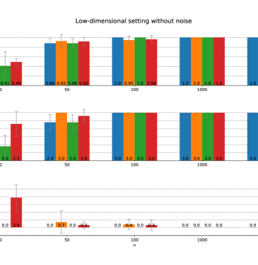
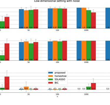
Figure 4: Low-dimensional setting, $d=8$ and $n\in\{10,50,100,1000,100000\}$. Evaluation results with no noise and noise ($\eta=0.5$) on regression coefficients, shown in upper and lower half, respectively.

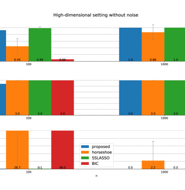
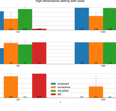
Figure 5: High-dimensional setting, $d=1000$ and $n\in\{100,1000\}$. Evaluation results with no noise and noise ($\eta=0.2$) on regression coefficients, shown in upper and lower half, respectively.

Table 2: Low-dimensional setting, $d=8$ and $n\in\{10,50,100,1000,100000\}$. Evaluation results with no noise on regression coefficients. For different $\delta$, comparison of the proposed method and product moment matching priors (MOM) from (Johnson and Rossell, 2012).

F1-Scores
	10	50	100	1000	100000
proposed ($\delta$ = 0.8)	0.47 (0.18)	0.88 (0.1)	1.0 (0.0)	1.0 (0.0)	1.0 (0.0)
proposed ($\delta$ = 0.5)	0.47 (0.18)	0.88 (0.1)	1.0 (0.0)	1.0 (0.0)	1.0 (0.0)
proposed ($\delta$ = 0.05)	0.47 (0.19)	0.89 (0.09)	1.0 (0.0)	1.0 (0.0)	1.0 (0.0)
proposed ($\delta$ = 0.01)	0.47 (0.19)	0.89 (0.09)	1.0 (0.0)	1.0 (0.0)	1.0 (0.0)
proposed ($\delta$ = 0.001)	0.48 (0.19)	0.87 (0.09)	0.98 (0.08)	1.0 (0.0)	1.0 (0.0)
MOM ($\delta$ = 0.8)	0.52 (0.2)	0.81 (0.13)	0.98 (0.06)	1.0 (0.0)	1.0 (0.0)
MOM ($\delta$ = 0.5)	0.53 (0.2)	0.88 (0.1)	1.0 (0.0)	1.0 (0.0)	1.0 (0.0)
MOM ($\delta$ = 0.05)	0.38 (0.25)	0.59 (0.14)	0.77 (0.23)	0.99 (0.04)	1.0 (0.0)
MOM ($\delta$ = 0.01)	0.0 (0.0)	0.55 (0.0)	0.55 (0.0)	0.55 (0.0)	0.97 (0.06)
MOM ($\delta$ = 0.001)	0.0 (0.0)	0.0 (0.0)	0.0 (0.0)	0.55 (0.0)	0.55 (0.0)
Average number of selected variables
	10	50	100	1000	100000
proposed ($\delta$ = 0.8)	1.9 (1.87)	2.4 (0.49)	3.0 (0.0)	3.0 (0.0)	3.0 (0.0)
proposed ($\delta$ = 0.5)	1.9 (1.87)	2.4 (0.49)	3.0 (0.0)	3.0 (0.0)	3.0 (0.0)
proposed ($\delta$ = 0.05)	2.3 (2.65)	2.6 (0.66)	3.0 (0.0)	3.0 (0.0)	3.0 (0.0)
proposed ($\delta$ = 0.01)	2.3 (2.65)	2.6 (0.66)	3.0 (0.0)	3.0 (0.0)	3.0 (0.0)
proposed ($\delta$ = 0.001)	3.0 (3.1)	2.5 (0.67)	3.2 (0.6)	3.0 (0.0)	3.0 (0.0)
MOM ($\delta$ = 0.8)	3.1 (2.77)	2.1 (0.54)	2.9 (0.3)	3.0 (0.0)	3.0 (0.0)
MOM ($\delta$ = 0.5)	3.0 (2.68)	2.4 (0.49)	3.0 (0.0)	3.0 (0.0)	3.0 (0.0)
MOM ($\delta$ = 0.05)	5.6 (3.67)	7.5 (1.5)	5.5 (2.5)	3.1 (0.3)	3.0 (0.0)
MOM ($\delta$ = 0.01)	0.0 (0.0)	8.0 (0.0)	8.0 (0.0)	8.0 (0.0)	3.2 (0.4)
MOM ($\delta$ = 0.001)	0.0 (0.0)	0.0 (0.0)	0.0 (0.0)	8.0 (0.0)	8.0 (0.0)

Table 3: Low-dimensional setting, $d=8$ and $n\in\{10,50,100,1000,100000\}$. Evaluation results with noise on regression coefficients $\eta=0.5$. For different $\delta$, comparison of the proposed method and product moment matching priors (MOM) from (Johnson and Rossell, 2012).

F1-Scores
	10	50	100	1000	100000
proposed ($\delta$ = 0.8)	0.36 (0.25)	0.85 (0.19)	0.97 (0.07)	1.0 (0.0)	1.0 (0.0)
proposed ($\delta$ = 0.5)	0.45 (0.18)	0.93 (0.09)	0.97 (0.07)	1.0 (0.0)	1.0 (0.0)
proposed ($\delta$ = 0.05)	0.34 (0.24)	0.93 (0.09)	0.95 (0.08)	0.8 (0.11)	0.6 (0.0)
proposed ($\delta$ = 0.01)	0.34 (0.24)	0.93 (0.09)	0.95 (0.08)	0.8 (0.11)	0.59 (0.02)
proposed ($\delta$ = 0.001)	0.34 (0.24)	0.93 (0.09)	0.95 (0.08)	0.8 (0.11)	0.59 (0.02)
MOM ($\delta$ = 0.8)	0.42 (0.24)	0.74 (0.21)	0.95 (0.08)	0.97 (0.06)	0.6 (0.0)
MOM ($\delta$ = 0.5)	0.46 (0.2)	0.81 (0.17)	0.97 (0.07)	0.96 (0.07)	0.6 (0.0)
MOM ($\delta$ = 0.05)	0.27 (0.27)	0.55 (0.0)	0.77 (0.23)	0.76 (0.1)	0.6 (0.0)
MOM ($\delta$ = 0.01)	0.0 (0.0)	0.55 (0.0)	0.55 (0.0)	0.55 (0.0)	0.58 (0.02)
MOM ($\delta$ = 0.001)	0.0 (0.0)	0.0 (0.0)	0.0 (0.0)	0.55 (0.0)	0.55 (0.0)
Average number of selected variables
	10	50	100	1000	100000
proposed ($\delta$ = 0.8)	2.4 (2.11)	2.5 (0.92)	3.0 (0.45)	3.0 (0.0)	3.0 (0.0)
proposed ($\delta$ = 0.5)	3.2 (2.36)	3.0 (0.63)	3.0 (0.45)	3.0 (0.0)	3.0 (0.0)
proposed ($\delta$ = 0.05)	2.5 (2.42)	3.0 (0.63)	3.1 (0.54)	4.6 (0.92)	7.0 (0.0)
proposed ($\delta$ = 0.01)	2.5 (2.42)	3.0 (0.63)	3.1 (0.54)	4.6 (0.92)	7.1 (0.3)
proposed ($\delta$ = 0.001)	2.5 (2.42)	3.0 (0.63)	3.1 (0.54)	4.6 (0.92)	7.1 (0.3)
MOM ($\delta$ = 0.8)	3.3 (2.57)	1.9 (0.83)	2.9 (0.54)	3.2 (0.4)	7.0 (0.0)
MOM ($\delta$ = 0.5)	3.4 (2.37)	2.5 (1.02)	3.0 (0.45)	3.3 (0.46)	7.0 (0.0)
MOM ($\delta$ = 0.05)	4.0 (4.0)	8.0 (0.0)	5.5 (2.5)	5.0 (0.89)	7.0 (0.0)
MOM ($\delta$ = 0.01)	0.0 (0.0)	8.0 (0.0)	8.0 (0.0)	8.0 (0.0)	7.3 (0.46)
MOM ($\delta$ = 0.001)	0.0 (0.0)	0.0 (0.0)	0.0 (0.0)	8.0 (0.0)	8.0 (0.0)

8 Evaluation on real data

In this section, we compare the results of our proposed and all baselines on two real data sets: crime data (Raftery et al., 1997; Liang et al., 2008) and ozone data (Garcia-Donato and Martinez-Beneito, 2013). Details of all datasets, preprocessing, and additional results on GDP growth data (SDM) (Sala-i Martin et al., 2004) are given in Appendix D.

We also show the results for AIC, the extended Bayesian information criterion (EBIC), stability selection, EMVS and the robust objective prior (Bayarri et al., 2012), which we denote as “GibbsBvs". Note that EBIC with $\gamma=0$, is equal to ordinary BIC (Schwarz, 1978). For the experiments with the real data we use 100000 MCMC-samples for the proposed method, GibbsBvs, and the horseshoe prior.

The results for the ozone and crime data are shown in Tables 4 and 5, respectively. We see that the horseshoe method performs similar as in the simulated data, tending to select models with relatively many variables. For ozone, our model suggests that the model using x6.x7, x6.x8, x7.x7, and x6.x6, have relatively high regression coefficients, but not all of them are together in one model, possibly due to high correlation. For crime, our model suggests that all variables should be considered as relevant, whereas in particular M, Ed, Po1, Ineq have high regression coefficients.

To further analyze the results of our proposed method, we inspect the top 10 model probabilities and variable inclusion probabilities calculated for $\delta=0$ and $\delta=0.5$. The model probabilities for ozone and crime are shown in Tables 6 and 8, respectively. Considering the low model probabilities, it is clear that there is no clearly winning model, and that care is needed when drawing conclusions from only the top model.

In order to investigate the importance of each individual variable, we also show the variable inclusion probabilities for ozone and crime in Tables 7 and 9, respectively. In each of the Tables, we also show the results that were reported in previous studies. From the difference in the probabilities between previous studies, $\delta=0$ and $\delta=0.5$, we can draw some interesting conclusions.

Ozone data

In Table 7, we show the inclusion probabilities of the proposed method together with the results reported in (Garcia-Donato and Martinez-Beneito, 2013). Comparing those results to the result of the proposed method, we find that the discrepancy between the results is not large, except in two cases. First, the importance of the variable x9, including its interaction terms, is much higher in (Garcia-Donato and Martinez-Beneito, 2013). Second, the squared term x7.x7 is considered as relevant by the proposed method, even when $\delta=0.5$, which is in contrast to (Garcia-Donato and Martinez-Beneito, 2013), where an inclusion probability of only $45\%$ is reported. Comparing the proposed method between $\delta=0.0$ and $\delta=0.5$, we see that the interaction variable x6.x8 is the most likely to be included for $\delta=0.0$, with probability around 70%. However, looking at the result with $\delta=0.5$, the effect size of x7.x7 is likely to be larger than x6.x8.

Crime data

In Table 9, we show the inclusion probabilities of the proposed method together with the results reported in (Liang et al., 2008). For the proposed method with $\delta=0$, we see good agreement with the results in (Liang et al., 2008). This is in particular true with respect to the median probability model that includes all variables with probability larger than or equal to 0.5. However, inspecting the inclusion probabilities for $\delta=0.5$, there is not enough evidence that the effect size of Po2 and U2 is high.

Table 4: Selected variables for the ozone data. For the proposed method and horseshoe method, we denote by "MSE inc" the expected increase in mean squared error compared to choosing the full model.

method	selected variables
proposed ($\delta$ = 0.8, MSE inc = 37.31%)	x7.x7
proposed ($\delta$ = 0.5, MSE inc = 19.5%)	x6.x6, x6.x7
proposed ($\delta$ = 0.05, MSE inc = 5.43%)	x6.x7, x6.x8, x7.x7
proposed ($\delta$ = 0.01, MSE inc = 4.91%)	x6.x6, x6.x7, x6.x8
proposed ($\delta$ = 0.001, MSE inc = 4.94%)	x6.x6, x6.x7, x6.x8
proposed ($\delta$ = 0.0, MSE inc = 5.44% )	x6.x7, x6.x8, x7.x7
horseshoe ($\delta$ = 0.8, MSE inc = 15.47%)	x6.x7, x7.x7, x7.x10
horseshoe ($\delta$ = 0.5, MSE inc = 5.11%)	x6.x7, x6.x8, x7.x7, x7.x8, x7.x10
horseshoe ($\delta$ = 0.05, MSE inc = 0.0%)	all except x5, x4.x5, x4.x8, x5.x8, x6.x9, x6.x10, x8.x8, x8.x9, x9.x10
horseshoe ($\delta$ = 0.01, MSE inc = 0.0%)	all except x5.x8, x6.x9
horseshoe ($\delta$ = 0.001, MSE inc = 0.0%)	all except x6.x9
horseshoe ($\delta$ = 0.0, MSE inc = 0.0%)	all
GibbsBvs	x6.x6, x6.x7, x6.x8
EMVS	none
SSLASSO	x6.x7, x6.x8, x7.x7
MOM ($\delta=0.8$)	x6.x6, x6.x7, x6.x8
MOM ($\delta=0.5$)	x6.x6, x6.x7, x6.x8
MOM ($\delta=0.05$)	all
AIC	x9, x4.x4, x6.x7, x6.x8, x7.x7, x7.x8, x7.x10, x8.x10, x9.x9
EBIC ($\gamma=0$)	x6.x7, x6.x8, x7.x7, x7.x8, x7.x10, x8.x10, x9.x9
EBIC ($\gamma=0.5$)	x6.x7, x7.x7, x7.x8, x7.x10, x9.x9
EBIC ($\gamma=1.0$)	x4.x8, x6.x7, x7.x7
stability ($q=0.1\cdot d$)	x7.x7
stability ($q=0.5\cdot d$)	x7.x10
stability ($q=0.8\cdot d$)	none

Table 5: Selected variables for the crime data. For the proposed method and horseshoe method, we denote by "MSE inc" the expected increase in mean squared error compared to choosing the full model.

method	selected variables
proposed ($\delta$ = 0.8, MSE inc = 65.62%)	Po1, Ineq
proposed ($\delta$ = 0.5, MSE inc = 21.97%)	M, Ed, Po1, Ineq
proposed ($\delta$ = 0.05, MSE inc = 0.0%)	all
proposed ($\delta$ = 0.01, MSE inc = 0.0%)	all
proposed ($\delta$ = 0.001, MSE inc = 0.0%)	all
proposed ($\delta$ = 0.0, MSE inc = 0.0%)	all
horseshoe ($\delta$ = 0.8, MSE inc = 17.23%)	M, Ed, Po1, Po2, NW, Ineq, Prob
horseshoe ($\delta$ = 0.5, MSE inc = 3.07%)	all except So, LF, M.F, Pop, U1, Time
horseshoe ($\delta$ = 0.05, MSE inc = 0.0%)	all except M.F
horseshoe ($\delta$ = 0.01, MSE inc = 0.0%)	all except M.F
horseshoe ($\delta$ = 0.001, MSE inc = 0.0%)	all
horseshoe ($\delta$ = 0.0, MSE inc = 0.0%)	all
GibbsBvs	all
EMVS	Po1, Ineq
SSLASSO	Ed, Po1, NW, Ineq
MOM ($\delta=0.8$)	Po1, Ineq
MOM ($\delta=0.5$)	Po1, Ineq
MOM ($\delta=0.05$)	all
AIC	all except So, Po2, M.F, U1
EBIC ($\gamma=0$)	all except So, Po2, LF, Pop, U1, GDP, Time
EBIC ($\gamma=0.5$)	M, Ed, Po1, M.F, NW, Ineq, Prob
EBIC ($\gamma=1.0$)	Po1, NW
stability ($q=0.1\cdot d$)	Po1
stability ($q=0.5\cdot d$)	NW
stability ($q=0.8\cdot d$)	none

Table 6: Top 10 selected models using the proposed method with $\delta=0.0$ and $\delta=0.5$ for the ozone data. Last column also shows the highest posterior probability model reported in (Garcia-Donato and Martinez-Beneito, 2013) using a $g$-prior where inclusion probabilities are calculated exactly (i.e. no MCMC).

model	probability
$\delta=0.5$
x6.x6, x6.x7	0.066
x6.x7, x7.x7	0.034
x4.x10, x7.x7, x7.x10	0.027
x7.x7	0.026
x10, x4.x7, x7.x10	0.02
x4.x7, x4.x10, x7.x10	0.019
x10, x7.x7, x7.x10	0.019
x7, x6.x7, x7.x7	0.016
x7.x7, x7.x10	0.015
x6.x6, x6.x7, x7.x8	0.013
$\delta=0.0$
x6.x7, x6.x8, x7.x7	0.031
x6.x6, x6.x7, x6.x8	0.029
x10, x6.x7, x6.x8, x7.x7, x7.x10	0.018
x4.x10, x6.x7, x6.x8, x7.x7, x7.x10	0.018
x4.x6, x4.x10, x6.x8, x7.x7, x7.x10	0.016
x10, x4.x6, x6.x8, x7.x7, x7.x10	0.013
x6.x7, x7.x7, x7.x8	0.01
x6, x4.x10, x6.x8, x7.x7, x7.x10	0.01
x4.x6, x6.x8, x7.x7	0.009
x6, x6.x8, x7.x7	0.009
Gracia-Donato
x10, x4.x6, x6.x8, x7.x7, x7.x10	0.0009

Table 7: All variable inclusion probabilities using the proposed method with $\delta=0.0$ and $\delta=0.5$ for the ozone data. Last column also shows the results reported in (Garcia-Donato and Martinez-Beneito, 2013) using a $g$-prior where inclusion probabilities are calculated exactly (i.e. no MCMC).

variable	$\delta=0.5$	$\delta=0.0$	Gracia-Donato
x7.x7	0.58	0.67	0.450
x6.x7	0.568	0.603	0.636
x7.x10	0.5	0.649	0.743
x6.x6	0.313	0.245	0.532
x4.x10	0.233	0.334	0.361
x6.x8	0.226	0.702	0.560
x10	0.226	0.291	0.368
x4.x7	0.212	0.234	0.252
x7.x8	0.179	0.279	0.349
x4.x6	0.164	0.295	0.325
x6	0.139	0.246	0.297
x7	0.133	0.16	0.195
x7.x9	0.09	0.072	0.431
x8	0.076	0.139	0.200
x4.x9	0.064	0.059	0.301
x4.x8	0.064	0.132	0.208
x9.x9	0.059	0.156	0.434
x9	0.053	0.056	0.291
x8.x10	0.037	0.112	0.236
x10.x10	0.028	0.07	0.117
x8.x8	0.028	0.067	0.142
x8.x9	0.019	0.034	0.263
x5.x10	0.019	0.036	0.124
x6.x10	0.017	0.052	0.115
x6.x9	0.012	0.036	0.126
x4.x4	0.011	0.032	0.164
x5.x6	0.011	0.027	0.107
x4	0.011	0.031	0.164
x5.x8	0.009	0.031	0.098
x5.x5	0.008	0.024	0.124
x5.x7	0.008	0.025	0.094
x9.x10	0.007	0.024	0.103
x5	0.006	0.019	0.096
x4.x5	0.006	0.02	0.095
x5.x9	0.005	0.022	0.088

Table 8: Top 10 selected models using the proposed method with $\delta=0.0$ and $\delta=0.5$ for the crime data.

model	probability
$\delta=0.5$
M, Ed, Po1, Ineq	0.021
M, Ed, Po1, NW, Ineq, Prob	0.017
Po1, Ineq	0.017
Ed, Po1, Ineq	0.016
M, Ed, Po1, NW, U2, Ineq, Prob	0.015
M, Ed, Po1, Ineq, Prob	0.015
Ed, Po1, NW, Ineq, Prob	0.013
M, Ed, Po1, U2, Ineq	0.011
M, Ed, Po1, U2, Ineq, Prob	0.011
M, Ed, Po1, NW, Ineq, Prob, Time	0.011
$\delta=0.0$
all	0.02
M, Ed, Po1, Ineq	0.01
M, Ed, Po1, NW, U2, Ineq, Prob	0.01
Ed, Po1, Ineq	0.008
M, Ed, Po1, NW, Ineq, Prob	0.008
all except So, Po2, LF, M.F, Pop, U1, GDP	0.008
Po1, Ineq	0.007
all except So, LF, M.F, Pop, U1, GDP, Time	0.007
M, Ed, Po1, NW, Ineq, Prob, Time	0.007
M, Ed, Po1, U2, Ineq, Prob	0.007

Table 9: All variable inclusion probabilities using the proposed method with $\delta=0.5$ and $\delta=0.0$ for the crime data. Last column also shows the results reported in (Liang et al., 2008) with the Zellner-Siow Prior with the null-model as the reference model.

variable	$\delta=0.5$	$\delta=0.0$	Liang
Ineq	0.993	0.995	1.0
Ed	0.906	0.943	0.97
Prob	0.758	0.833	0.90
Po1	0.742	0.792	0.67
M	0.731	0.808	0.85
NW	0.604	0.711	0.69
Po2	0.52	0.591	0.45
U2	0.425	0.557	0.61
GDP	0.381	0.481	0.36
Time	0.256	0.395	0.37
Pop	0.244	0.368	0.37
So	0.207	0.32	0.27
U1	0.134	0.269	0.25
M.F	0.12	0.238	0.20
LF	0.115	0.233	0.20

9 Conclusions

We proposed a new type of spike-and-slab prior that is particularly well suited for the situation where there are small negligible, but non-zero regression coefficients (quasi-sparseness). These small negligible regression coefficients are considered as noise, since they can lead to the selection of overly complex models (i.e. models with many variables), although, only few variables should be considered as practically relevant. The proposed method uses disjunct support priors on the regression coefficients with a threshold parameter $\delta>0$ in order to ignore small coefficients. We showed that in the quasi-sparse setting, the proposed method leads to consistent Bayes factors, which is not the case for full support priors as originally proposed in (Chipman et al., 2001), and the moment matching priors (MOM) (Johnson and Rossell, 2010, 2012; Rossell and Telesca, 2017).

Due to the non-conjugacy of the priors proposed by our method, estimating the marginal likelihood explicitly is computationally infeasible. We therefore introduced a latent variable indicator vector $\mathbf{z}$, and proposed an efficient Gibbs sampler to sample from its posterior distribution.

For synthetic data with ground truth, we showed that the proposed method leads to good model selection performance in various settings: with/without noise and low/high dimensions. For real data, we showed that by inspecting the model and variable inclusion probabilities for different threshold values $\delta$, we can draw interesting conclusions about the effect size (the absolute magnitude) of regression coefficients. Together with an estimate of the mean squared error (MSE) of the final model, this allows for a trade-off between sparsity and prediction accuracy, similar to the practical advise given in (Hahn and Carvalho, 2015).

Appendix A: Asymptotic Results

Lemma 1.

The function

$$\boldsymbol{\theta}\rightarrow\operatorname{\mathbb{E}}_{\mathbf{x}}\Big{[}g(\boldsymbol{\theta})\Big{]}\,,$$

has a unique maximum, where

$$g(\boldsymbol{\theta}):=\operatorname{\mathbb{E}}_{y\sim p(y|\boldsymbol{\theta},\mathbf{x})}\Big{[}\log p(y|\boldsymbol{\theta},\mathbf{x})\Big{]}\,.$$

and $\mathbf{x}$ is distributed according to some non-degenerated distribution with mean zero and positive definite covariance matrix $C$.

Proof.

First of all, let us do a change of variable using the one-to-one mapping $\tau:=\sigma_{r}^{-2}$. For simplicity, let us denote $\boldsymbol{\theta}:=(\tau,\boldsymbol{\beta})$, and the true parameter vector as $\boldsymbol{\theta}_{t}$. We have

$$\log p(y|\boldsymbol{\theta},\mathbf{x})=\frac{1}{2}\log\tau-\frac{1}{2}\tau(y-\mathbf{x}^{T}\boldsymbol{\beta})^{2}-\frac{1}{2}\log 2\pi\,,$$

and

$$\operatorname{\mathbb{E}}_{\mathbf{x}}\Big{[}g(\boldsymbol{\theta})\Big{]}=\operatorname{\mathbb{E}}_{\mathbf{x},y}\Big{[}\log p(y|\boldsymbol{\theta},\mathbf{x})\Big{]}=\frac{1}{2}\log\tau-\frac{1}{2}\tau\operatorname{\mathbb{E}}_{\mathbf{x},y}\Big{[}(y-\mathbf{x}^{T}\boldsymbol{\beta})^{2}\Big{]}-\frac{1}{2}\log 2\pi\,.$$

Since $C$ is positive definite, we have that $\operatorname{\mathbb{E}}_{\mathbf{x},y}\Big{[}(y-\mathbf{x}^{T}\boldsymbol{\beta})^{2}\Big{]}$ has a unique minimum at $\boldsymbol{\beta}=\boldsymbol{\beta}_{t}$. To see this note that

$$\operatorname{\mathbb{E}}_{\mathbf{x},y}\Big{[}(y-\mathbf{x}^{T}\boldsymbol{\beta})^{2}\Big{]} =\operatorname{\mathbb{E}}_{\mathbf{x},\epsilon}\Big{[}(\mathbf{x}^{T}\boldsymbol{\beta}_{t}+\epsilon-\mathbf{x}^{T}\boldsymbol{\beta})^{2}\Big{]}$$

$$=\operatorname{\mathbb{E}}_{\mathbf{x},\epsilon}\Big{[}\big{(}\mathbf{x}^{T}(\boldsymbol{\beta}_{t}-\boldsymbol{\beta})+\epsilon\big{)}^{2}\Big{]}$$

$$=\operatorname{\mathbb{E}}_{\mathbf{x}}\Big{[}\big{(}\mathbf{x}^{T}(\boldsymbol{\beta}_{t}-\boldsymbol{\beta})\big{)}^{2}\Big{]}+2\operatorname{\mathbb{E}}_{\mathbf{x},\epsilon}\Big{[}\epsilon\cdot\mathbf{x}^{T}(\boldsymbol{\beta}_{t}-\boldsymbol{\beta})\Big{]}+E_{\epsilon}\Big{[}\epsilon^{2}\Big{]}$$

$$=(\boldsymbol{\beta}_{t}-\boldsymbol{\beta})^{T}\operatorname{\mathbb{E}}_{\mathbf{x}}\Big{[}\mathbf{x}\mathbf{x}^{T}\Big{]}(\boldsymbol{\beta}_{t}-\boldsymbol{\beta})+2\operatorname{\mathbb{E}}_{\epsilon}\Big{[}\epsilon\Big{]}\cdot\operatorname{\mathbb{E}}_{\mathbf{x}}\Big{[}\mathbf{x}^{T}\Big{]}(\boldsymbol{\beta}_{t}-\boldsymbol{\beta})+E_{\epsilon}\Big{[}\epsilon^{2}\Big{]}$$

$$=(\boldsymbol{\beta}_{t}-\boldsymbol{\beta})^{T}C(\boldsymbol{\beta}_{t}-\boldsymbol{\beta})+\sigma_{r,t}^{2}\,.$$

where we used that $\operatorname{\mathbb{E}}_{\mathbf{x}}\Big{[}\mathbf{x}\Big{]}=\mathbf{0}$, and $C=\operatorname{\mathbb{E}}_{\mathbf{x}}\Big{[}\mathbf{x}\mathbf{x}^{T}\Big{]}$. For $\boldsymbol{\beta}=\boldsymbol{\beta}_{t}$, we have $\operatorname{\mathbb{E}}_{\mathbf{x},y}\Big{[}(y-\mathbf{x}^{T}\boldsymbol{\beta})^{2}\Big{]}=\frac{1}{\tau_{t}}$. Furthermore, since

$$\operatorname{\mathbb{E}}_{\mathbf{x}}\Big{[}g(\tau,\boldsymbol{\beta}_{t})\Big{]}=\frac{1}{2}\log\tau-\frac{1}{2}\tau\frac{1}{\tau_{t}}-\frac{1}{2}\log 2\pi$$

is strictly concave with respect to $\tau$, with unique maximum $\tau_{r}$, we have that the unique maximum of $\operatorname{\mathbb{E}}_{\mathbf{x}}\Big{[}g(\boldsymbol{\theta})\Big{]}$ is given by $(\tau_{t},\boldsymbol{\beta}_{t})$. ∎

Appendix B: Slice Sampler

First let us introduce the auxiliary random variable $U$, and the following joint distribution:

$$p(U,\sigma^{2}_{1})=\begin{cases}\frac{1}{L}\cdot\text{Inv-}\chi^{2}(\sigma^{2}_{1}|\tilde{\nu},\tilde{\eta}^{2})&\text{if }0<U<h(\sigma^{2}_{1}),\\ 0&\text{else. }\end{cases}\,,$$

where $L$ is an appropriate normalization constant. We then have that

$$p(\sigma^{2}_{1}) =\int_{0}^{h(\sigma^{2}_{1})}p(u,\sigma^{2}_{1})du$$

$$=\frac{1}{L}\cdot\text{Inv-}\chi^{2}(\sigma^{2}_{1}|\tilde{\nu},\tilde{\eta}^{2})\int_{0}^{h(\sigma^{2}_{1})}1du$$

$$=\frac{1}{L}\cdot\text{Inv-}\chi^{2}(\sigma^{2}_{1}|\tilde{\nu},\tilde{\eta}^{2})\big{[}u\big{]}_{0}^{h(\sigma^{2}_{1})}$$

$$=\frac{1}{L}\cdot h(\sigma^{2}_{1})\cdot\text{Inv-}\chi^{2}(\sigma^{2}_{1}|\tilde{\nu},\tilde{\eta}^{2})$$

$$\propto h(\sigma^{2}_{1})\cdot\text{Inv-}\chi^{2}(\sigma^{2}_{1}|\tilde{\nu},\tilde{\eta}^{2})$$

In order to sample from the joint distribution $p(U,\sigma^{2}_{1})$, we employ a Gibbs sampler, where

$$p(U|\sigma^{2}_{1})=\text{Uniform}([0,h(\sigma^{2}_{1})])$$

and

$$p(\sigma^{2}_{1}|u)=\begin{cases}\frac{1}{\tilde{L}}\cdot\text{Inv-}\chi^{2}(\sigma^{2}_{1}|\tilde{\nu},\tilde{\eta}^{2})&\text{if }h(\sigma^{2}_{1})>u,\\ 0&\text{else. }\end{cases}\,,$$

for an appropriate normalization constant $\tilde{L}$.

Appendix C: Additional results synthetic data

We show the results for $\delta\in\{0.8,0.5,0.05,0.01,0.001,0.0\}$, and the results of the most parsimonious model that is estimated to lead to an increase in MSE of not more than 5%. For all methods based on MCMC we use 10000 samples, out of which 10% are used for burn in.

As our first baseline, we use the robust objective prior proposed in (Bayarri et al., 2012) together with a Gibbs sampler to explore the space of models, which we denote as “GibbsBvs". Furthermore, we use the Gaussian and Laplace spike-and-slab priors combined with EM-algorithm as proposed in (Ročková and George, 2014, 2018) which we denote as "EMVS" and "SSLASSO", respectively. Note that EMVS and SSLASSO do not provide model or variable inclusion posterior probabilities.

Finally, we include also three frequentist methods for model search. As a first frequentist method, we use the popular Least Angle Regression (LARS) method (Efron et al., 2004) to get a set of candidate models. We then select the model using the Extended Bayesian information criterion (EBIC) with $\gamma\in\{0,0.5,1\}$ (Chen and Chen, 2008; Foygel and Drton, 2010), or the Akaike information criterion (AIC) (Akaike, 1973). Note that EBIC with $\gamma=0$, is equal to the Bayesian information criterion (BIC) (Schwarz, 1978). As a third frequentist method, we use linear regression with Lasso (Tibshirani, 1996) combined with stability selection (Meinshausen and Bühlmann, 2010). Stability selection has two hyper-parameters that need to be specified: the "upper bound for the per-family error rate" (PFER) and "the number of (unique) selected variables" (denoted by $q$) as in the R package ’stabs’. For PFER we set always 1. However, we found that stability selection can be sensitive to the choice of $q$, and therefore show all results for three different values.

We evaluate all methods in terms of F1-Score. All experiments are repeated 10 times and we report average and standard deviations (shown in brackets). For large $n$, GibbsBvs did not execute correctly, which we mark as "-". For the high-dimensional setting GibbsBvs did not finish computation due to high memory requirements. When we selected the threshold value $\delta$ automatically by using the estimated increase in MSE, we mark this in all Tables by "^∗". If not reported otherwise, we use for all baselines the default settings.

Low-dimensional setting

The results for the low-dimensional setting, with and without noise, are shown in Tables 10, 11 and 12. Overall, we see that the proposed method and the horseshoe prior method perform best.

GibbsBvs, SSLASSO, EBIC and Stability selection (with $q\geq 4$) perform good for no noise or small noise. However, for $\eta=0.5$, GibbsBvs, SSLASSO, EBIC and Stability Selection start to select more irrelevant variables with increasing sample size $n$. Asymptotically, all four methods are expected to select all variables with coefficient regressions $\beta_{j}\neq 0$, no matter how small $\beta_{j}$ is. However, if the sample size is small ($n\leq 100$), then all three methods are not influenced by the noise, i.e. they ignore the negligible small regression coefficients.

AIC performs similar to EBIC for $n\leq 100$, but for larger sample sizes it tends to select too many variables, even in the no-noise setting. This is not too surprising, since it is well known that AIC is not model selection consistent (see e.g. (Yang, 2005)).

Interestingly, in the noise setting ($\eta=0.2$ and $\eta=0.5$), even for large $n$, EMVS find the correct relevant variables. However, for small sample sizes EMVS tends to select too few variables. This suggests that EMVS has a strong inductive bias for sparse models, which can be helpful in the noise setting, but is deteriorating performance for small to medium-sized $n$.

High-dimensional setting

The results for the high-dimensional setting, with and without noise, are shown in Tables 16, and 17. Overall, we see that the proposed method, SSLASSO, Stability selection (with $q\geq 50$) and EMVS perform best. In this setting the EMVS seems to profit from its inductive bias for sparse models. On the other hand, the horseshoe prior method performs somehow unsatisfactory, tending to select too many variables. AIC and EBIC performed very poorly in this setting, selecting too many variables. One reason seems to stem from the numerical instability of the maximum likelihood estimate for $d\leq n$. As an ad-hoc remedy we tried to combine it with a ridge estimate, but this did not seem to help.

Analysis of different $\delta$

In Tables 13, 14, and 15, we show the results for different fixed $\delta$ in the low-dimensional setting, and in Tables 18 and 19 for the high-dimensional setting. The proposed method is less sensitive to the choice of $\delta$ and tends to select sparse models even in the high-dimensional setting. However, as expected, the horseshoe prior method is highly sensitive to the choice of $\delta$.

Comparison to moment matching priors

In Tables 20 and 21, we show the comparison of the proposed method and the product moment matching priors (MOM) from (Johnson and Rossell, 2012) for the high-dimensional settings. Similar to the low-dimensional setting, we observe that for small values of the practical relevance threshold $\delta$, MOM tends to select too few or too many variables.

Table 10: Low-dimensional setting, $d=8$ and $n\in\{10,50,100,1000,100000\}$. Evaluation results with no noise on regression coefficients.

F1-Scores
	10	50	100	1000	100000
proposed∗	0.48 (0.18)	0.88 (0.1)	1.0 (0.0)	1.0 (0.0)	1.0 (0.0)
horseshoe∗	0.59 (0.1)	0.93 (0.14)	0.95 (0.09)	1.0 (0.0)	1.0 (0.0)
GibbsBvs	0.48 (0.16)	0.89 (0.09)	0.95 (0.09)	1.0 (0.0)	-
EMVS	0.25 (0.25)	0.13 (0.27)	0.0 (0.0)	0.96 (0.08)	1.0 (0.0)
SSLASSO	0.41 (0.29)	0.88 (0.1)	1.0 (0.0)	1.0 (0.0)	1.0 (0.0)
AIC	0.49 (0.07)	0.89 (0.1)	0.88 (0.13)	0.88 (0.09)	0.85 (0.15)
EBIC ($\gamma=0.0$)	0.49 (0.07)	0.92 (0.09)	0.96 (0.08)	1.0 (0.0)	1.0 (0.0)
EBIC ($\gamma=0.5$)	0.53 (0.08)	0.91 (0.1)	1.0 (0.0)	1.0 (0.0)	1.0 (0.0)
EBIC ($\gamma=1.0$)	0.47 (0.16)	0.9 (0.1)	1.0 (0.0)	1.0 (0.0)	1.0 (0.0)
stability ($q=1$)	0.2 (0.24)	0.3 (0.24)	0.35 (0.23)	0.5 (0.0)	0.5 (0.0)
stability ($q=4$)	0.1 (0.2)	0.9 (0.1)	0.98 (0.06)	1.0 (0.0)	1.0 (0.0)
stability ($q=6$)	0.05 (0.15)	0.91 (0.1)	0.99 (0.04)	1.0 (0.0)	1.0 (0.0)
Average number of selected variables
	10	50	100	1000	100000
proposed∗	2.6 (2.58)	2.4 (0.49)	3.0 (0.0)	3.0 (0.0)	3.0 (0.0)
horseshoe∗	4.6 (2.2)	3.7 (1.49)	3.4 (0.66)	3.0 (0.0)	3.0 (0.0)
GibbsBvs	5.1 (3.56)	2.6 (0.66)	3.4 (0.66)	3.0 (0.0)	-
EMVS	0.5 (0.5)	0.3 (0.64)	0.0 (0.0)	2.8 (0.4)	3.0 (0.0)
SSLASSO	0.9 (0.7)	2.4 (0.49)	3.0 (0.0)	3.0 (0.0)	3.0 (0.0)
AIC	6.2 (2.4)	3.8 (0.75)	4.0 (1.18)	3.9 (0.7)	4.3 (1.49)
EBIC ($\gamma=0.0$)	6.2 (2.4)	3.1 (0.7)	3.3 (0.64)	3.0 (0.0)	3.0 (0.0)
EBIC ($\gamma=0.5$)	5.2 (2.89)	2.7 (0.64)	3.0 (0.0)	3.0 (0.0)	3.0 (0.0)
EBIC ($\gamma=1.0$)	3.8 (3.19)	2.5 (0.5)	3.0 (0.0)	3.0 (0.0)	3.0 (0.0)
stability ($q=1$)	0.4 (0.49)	0.6 (0.49)	0.7 (0.46)	1.0 (0.0)	1.0 (0.0)
stability ($q=4$)	0.2 (0.4)	2.5 (0.5)	2.9 (0.3)	3.0 (0.0)	3.0 (0.0)
stability ($q=6$)	0.1 (0.3)	2.7 (0.64)	3.1 (0.3)	3.0 (0.0)	3.0 (0.0)

Table 11: Low-dimensional setting, $d=8$ and $n\in\{10,50,100,1000,100000\}$. Evaluation results with noise on regression coefficients $\eta=0.2$.

F1-Scores
	10	50	100	1000	100000
proposed∗	0.41 (0.16)	0.95 (0.08)	0.97 (0.07)	1.0 (0.0)	1.0 (0.0)
horseshoe∗	0.6 (0.21)	0.88 (0.13)	0.99 (0.04)	1.0 (0.0)	1.0 (0.0)
GibbsBvs	0.49 (0.09)	0.93 (0.09)	0.97 (0.06)	0.99 (0.04)	-
EMVS	0.21 (0.26)	0.05 (0.15)	0.0 (0.0)	1.0 (0.0)	1.0 (0.0)
SSLASSO	0.28 (0.23)	0.86 (0.21)	0.97 (0.07)	1.0 (0.0)	0.63 (0.03)
AIC	0.56 (0.14)	0.87 (0.09)	0.87 (0.11)	0.81 (0.15)	0.58 (0.02)
EBIC ($\gamma=0.0$)	0.56 (0.13)	0.92 (0.09)	0.97 (0.06)	1.0 (0.0)	0.63 (0.03)
EBIC ($\gamma=0.5$)	0.55 (0.14)	0.91 (0.12)	0.99 (0.04)	1.0 (0.0)	0.63 (0.03)
EBIC ($\gamma=1.0$)	0.54 (0.14)	0.91 (0.12)	0.97 (0.07)	1.0 (0.0)	0.64 (0.03)
stability ($q=1$)	0.1 (0.2)	0.35 (0.23)	0.5 (0.0)	0.5 (0.0)	0.5 (0.0)
stability ($q=4$)	0.1 (0.2)	0.89 (0.16)	0.98 (0.06)	1.0 (0.0)	0.93 (0.07)
stability ($q=6$)	0.0 (0.0)	0.89 (0.2)	1.0 (0.0)	0.99 (0.04)	0.67 (0.0)
Average number of selected variables
	10	50	100	1000	100000
proposed∗	2.5 (2.06)	2.9 (0.54)	3.0 (0.45)	3.0 (0.0)	3.0 (0.0)
horseshoe∗	4.8 (2.23)	3.8 (1.54)	3.1 (0.3)	3.0 (0.0)	3.0 (0.0)
GibbsBvs	5.7 (2.9)	3.0 (0.63)	3.2 (0.4)	3.1 (0.3)	-
EMVS	1.1 (2.02)	0.1 (0.3)	0.0 (0.0)	3.0 (0.0)	3.0 (0.0)
SSLASSO	1.1 (0.94)	2.7 (0.78)	3.0 (0.45)	3.0 (0.0)	6.6 (0.49)
AIC	6.6 (2.15)	3.7 (0.9)	4.0 (1.1)	4.7 (1.49)	7.3 (0.46)
EBIC ($\gamma=0.0$)	6.5 (2.2)	3.1 (0.7)	3.2 (0.4)	3.0 (0.0)	6.6 (0.49)
EBIC ($\gamma=0.5$)	5.1 (2.7)	2.9 (0.54)	3.1 (0.3)	3.0 (0.0)	6.6 (0.49)
EBIC ($\gamma=1.0$)	4.5 (2.87)	2.9 (0.54)	3.0 (0.45)	3.0 (0.0)	6.4 (0.49)
stability ($q=1$)	0.3 (0.46)	0.7 (0.46)	1.0 (0.0)	1.0 (0.0)	1.0 (0.0)
stability ($q=4$)	0.2 (0.4)	2.5 (0.67)	2.9 (0.3)	3.0 (0.0)	3.5 (0.5)
stability ($q=6$)	0.0 (0.0)	2.7 (0.9)	3.0 (0.0)	3.1 (0.3)	6.0 (0.0)

Table 12: Low-dimensional setting, $d=8$ and $n\in\{10,50,100,1000,100000\}$. Evaluation results with noise on regression coefficients $\eta=0.5$.

F1-Scores
	10	50	100	1000	100000
proposed∗	0.47 (0.18)	0.93 (0.09)	0.97 (0.07)	1.0 (0.0)	1.0 (0.0)
horseshoe∗	0.63 (0.19)	0.88 (0.13)	0.97 (0.06)	1.0 (0.0)	1.0 (0.0)
GibbsBvs	0.49 (0.09)	0.87 (0.14)	0.96 (0.07)	0.78 (0.09)	-
EMVS	0.21 (0.26)	0.05 (0.15)	0.0 (0.0)	0.98 (0.06)	1.0 (0.0)
SSLASSO	0.35 (0.24)	0.9 (0.16)	0.97 (0.07)	0.88 (0.1)	0.6 (0.0)
AIC	0.56 (0.13)	0.83 (0.09)	0.9 (0.08)	0.64 (0.08)	0.55 (0.02)
EBIC ($\gamma=0.0$)	0.56 (0.13)	0.92 (0.09)	0.96 (0.07)	0.77 (0.14)	0.6 (0.0)
EBIC ($\gamma=0.5$)	0.56 (0.14)	0.91 (0.12)	0.95 (0.08)	0.82 (0.14)	0.6 (0.0)
EBIC ($\gamma=1.0$)	0.55 (0.14)	0.91 (0.12)	0.97 (0.07)	0.9 (0.1)	0.6 (0.0)
stability ($q=1$)	0.1 (0.2)	0.35 (0.23)	0.5 (0.0)	0.5 (0.0)	0.5 (0.0)
stability ($q=4$)	0.0 (0.0)	0.91 (0.16)	0.98 (0.06)	0.97 (0.06)	0.9 (0.07)
stability ($q=6$)	0.0 (0.0)	0.9 (0.16)	0.99 (0.04)	0.91 (0.07)	0.67 (0.0)
Average number of selected variables
	10	50	100	1000	100000
proposed∗	3.2 (2.23)	3.0 (0.63)	3.0 (0.45)	3.0 (0.0)	3.0 (0.0)
horseshoe∗	5.1 (2.62)	3.8 (1.54)	3.2 (0.4)	3.0 (0.0)	3.0 (0.0)
GibbsBvs	5.6 (2.84)	3.6 (1.62)	3.3 (0.46)	4.8 (0.75)	-
EMVS	1.1 (2.02)	0.1 (0.3)	0.0 (0.0)	2.9 (0.3)	3.0 (0.0)
SSLASSO	1.4 (1.02)	2.7 (0.78)	3.0 (0.45)	3.9 (0.83)	7.0 (0.0)
AIC	6.5 (2.2)	4.1 (1.14)	3.7 (0.64)	6.5 (1.02)	7.9 (0.3)
EBIC ($\gamma=0.0$)	6.5 (2.2)	3.1 (0.7)	3.3 (0.46)	5.0 (1.26)	7.0 (0.0)
EBIC ($\gamma=0.5$)	5.7 (2.37)	2.9 (0.54)	3.1 (0.54)	4.5 (1.28)	7.0 (0.0)
EBIC ($\gamma=1.0$)	4.3 (2.65)	2.9 (0.54)	3.0 (0.45)	3.8 (0.87)	7.0 (0.0)
stability ($q=1$)	0.3 (0.46)	0.7 (0.46)	1.0 (0.0)	1.0 (0.0)	1.0 (0.0)
stability ($q=4$)	0.0 (0.0)	2.6 (0.66)	2.9 (0.3)	3.2 (0.4)	3.7 (0.46)
stability ($q=6$)	0.0 (0.0)	2.7 (0.78)	3.1 (0.3)	3.6 (0.49)	6.0 (0.0)

Table 13: Low-dimensional setting, $d=8$ and $n\in\{10,50,100,1000,100000\}$. Evaluation results with no noise on regression coefficients. Comparison of the proposed method and horseshoe for different $\delta$.

F1-Scores
	10	50	100	1000	100000
proposed ($\delta$ = 0.8)	0.47 (0.18)	0.88 (0.1)	1.0 (0.0)	1.0 (0.0)	1.0 (0.0)
proposed ($\delta$ = 0.5)	0.47 (0.18)	0.88 (0.1)	1.0 (0.0)	1.0 (0.0)	1.0 (0.0)
proposed ($\delta$ = 0.05)	0.47 (0.19)	0.89 (0.09)	1.0 (0.0)	1.0 (0.0)	1.0 (0.0)
proposed ($\delta$ = 0.01)	0.47 (0.19)	0.89 (0.09)	1.0 (0.0)	1.0 (0.0)	1.0 (0.0)
proposed ($\delta$ = 0.001)	0.48 (0.19)	0.87 (0.09)	0.98 (0.08)	1.0 (0.0)	1.0 (0.0)
proposed ($\delta$ = 0.0)	0.47 (0.19)	0.87 (0.09)	0.99 (0.04)	1.0 (0.0)	1.0 (0.0)
proposed∗	0.48 (0.18)	0.88 (0.1)	1.0 (0.0)	1.0 (0.0)	1.0 (0.0)
horseshoe ($\delta$ = 0.8)	0.67 (0.14)	0.91 (0.1)	0.99 (0.04)	1.0 (0.0)	1.0 (0.0)
horseshoe ($\delta$ = 0.5)	0.7 (0.14)	0.94 (0.08)	0.95 (0.09)	1.0 (0.0)	1.0 (0.0)
horseshoe ($\delta$ = 0.05)	0.55 (0.05)	0.6 (0.04)	0.63 (0.09)	0.71 (0.13)	1.0 (0.0)
horseshoe ($\delta$ = 0.01)	0.53 (0.04)	0.56 (0.02)	0.56 (0.02)	0.59 (0.04)	0.84 (0.13)
horseshoe ($\delta$ = 0.001)	0.55 (0.0)	0.55 (0.02)	0.55 (0.0)	0.55 (0.0)	0.56 (0.02)
horseshoe ($\delta$ = 0.0)	0.55 (0.0)	0.55 (0.0)	0.55 (0.0)	0.55 (0.0)	0.55 (0.0)
horseshoe∗	0.59 (0.1)	0.93 (0.14)	0.95 (0.09)	1.0 (0.0)	1.0 (0.0)
Average number of selected variables
	10	50	100	1000	100000
proposed ($\delta$ = 0.8)	1.9 (1.87)	2.4 (0.49)	3.0 (0.0)	3.0 (0.0)	3.0 (0.0)
proposed ($\delta$ = 0.5)	1.9 (1.87)	2.4 (0.49)	3.0 (0.0)	3.0 (0.0)	3.0 (0.0)
proposed ($\delta$ = 0.05)	2.3 (2.65)	2.6 (0.66)	3.0 (0.0)	3.0 (0.0)	3.0 (0.0)
proposed ($\delta$ = 0.01)	2.3 (2.65)	2.6 (0.66)	3.0 (0.0)	3.0 (0.0)	3.0 (0.0)
proposed ($\delta$ = 0.001)	3.0 (3.1)	2.5 (0.67)	3.2 (0.6)	3.0 (0.0)	3.0 (0.0)
proposed ($\delta$ = 0.0)	2.3 (2.65)	2.5 (0.67)	3.1 (0.3)	3.0 (0.0)	3.0 (0.0)
proposed∗	2.6 (2.58)	2.4 (0.49)	3.0 (0.0)	3.0 (0.0)	3.0 (0.0)
horseshoe ($\delta$ = 0.8)	2.6 (0.92)	2.7 (0.64)	3.1 (0.3)	3.0 (0.0)	3.0 (0.0)
horseshoe ($\delta$ = 0.5)	3.6 (0.92)	3.2 (0.6)	3.4 (0.66)	3.0 (0.0)	3.0 (0.0)
horseshoe ($\delta$ = 0.05)	7.6 (0.49)	7.1 (0.7)	6.6 (1.11)	5.7 (1.35)	3.0 (0.0)
horseshoe ($\delta$ = 0.01)	7.9 (0.3)	7.7 (0.46)	7.7 (0.46)	7.2 (0.75)	4.3 (1.27)
horseshoe ($\delta$ = 0.001)	8.0 (0.0)	7.9 (0.3)	8.0 (0.0)	8.0 (0.0)	7.7 (0.46)
horseshoe ($\delta$ = 0.0)	8.0 (0.0)	8.0 (0.0)	8.0 (0.0)	8.0 (0.0)	8.0 (0.0)
horseshoe∗	4.6 (2.2)	3.7 (1.49)	3.4 (0.66)	3.0 (0.0)	3.0 (0.0)

Table 14: Low-dimensional setting, $d=8$ and $n\in\{10,50,100,1000,100000\}$. Evaluation results with noise on regression coefficients $\eta=0.2$. Comparison of the proposed method and horseshoe for different $\delta$.

F1-Scores
	10	50	100	1000	100000
proposed ($\delta$ = 0.8)	0.39 (0.22)	0.87 (0.19)	0.97 (0.07)	1.0 (0.0)	1.0 (0.0)
proposed ($\delta$ = 0.5)	0.4 (0.16)	0.95 (0.08)	0.97 (0.07)	1.0 (0.0)	1.0 (0.0)
proposed ($\delta$ = 0.05)	0.39 (0.22)	0.95 (0.08)	0.99 (0.04)	1.0 (0.0)	0.68 (0.04)
proposed ($\delta$ = 0.01)	0.4 (0.22)	0.95 (0.08)	0.99 (0.04)	0.99 (0.04)	0.62 (0.03)
proposed ($\delta$ = 0.001)	0.38 (0.21)	0.95 (0.08)	0.99 (0.04)	0.99 (0.04)	0.62 (0.03)
proposed ($\delta$ = 0.0)	0.37 (0.2)	0.95 (0.08)	0.99 (0.04)	0.99 (0.04)	0.62 (0.03)
proposed∗	0.41 (0.16)	0.95 (0.08)	0.97 (0.07)	1.0 (0.0)	1.0 (0.0)
horseshoe ($\delta$ = 0.8)	0.61 (0.29)	0.95 (0.08)	0.99 (0.04)	1.0 (0.0)	1.0 (0.0)
horseshoe ($\delta$ = 0.5)	0.59 (0.29)	0.92 (0.08)	0.99 (0.04)	1.0 (0.0)	1.0 (0.0)
horseshoe ($\delta$ = 0.05)	0.59 (0.11)	0.61 (0.1)	0.62 (0.06)	0.65 (0.07)	0.66 (0.04)
horseshoe ($\delta$ = 0.01)	0.55 (0.0)	0.56 (0.04)	0.56 (0.02)	0.57 (0.03)	0.58 (0.03)
horseshoe ($\delta$ = 0.001)	0.55 (0.0)	0.55 (0.0)	0.55 (0.0)	0.55 (0.0)	0.55 (0.0)
horseshoe ($\delta$ = 0.0)	0.55 (0.0)	0.55 (0.0)	0.55 (0.0)	0.55 (0.0)	0.55 (0.0)
horseshoe∗	0.6 (0.21)	0.88 (0.13)	0.99 (0.04)	1.0 (0.0)	1.0 (0.0)
Average number of selected variables
	10	50	100	1000	100000
proposed ($\delta$ = 0.8)	2.5 (2.16)	2.6 (0.92)	3.0 (0.45)	3.0 (0.0)	3.0 (0.0)
proposed ($\delta$ = 0.5)	2.6 (2.06)	2.9 (0.54)	3.0 (0.45)	3.0 (0.0)	3.0 (0.0)
proposed ($\delta$ = 0.05)	2.5 (2.25)	2.9 (0.54)	3.1 (0.3)	3.0 (0.0)	5.9 (0.54)
proposed ($\delta$ = 0.01)	2.8 (2.6)	2.9 (0.54)	3.1 (0.3)	3.1 (0.3)	6.7 (0.46)
proposed ($\delta$ = 0.001)	2.6 (2.46)	2.9 (0.54)	3.1 (0.3)	3.1 (0.3)	6.7 (0.46)
proposed ($\delta$ = 0.0)	2.7 (2.61)	2.9 (0.54)	3.1 (0.3)	3.1 (0.3)	6.7 (0.46)
proposed∗	2.5 (2.06)	2.9 (0.54)	3.0 (0.45)	3.0 (0.0)	3.0 (0.0)
horseshoe ($\delta$ = 0.8)	3.1 (1.04)	2.9 (0.54)	3.1 (0.3)	3.0 (0.0)	3.0 (0.0)
horseshoe ($\delta$ = 0.5)	3.8 (0.98)	3.3 (0.64)	3.1 (0.3)	3.0 (0.0)	3.0 (0.0)
horseshoe ($\delta$ = 0.05)	7.1 (1.22)	7.0 (1.34)	6.7 (0.9)	6.4 (1.02)	6.1 (0.54)
horseshoe ($\delta$ = 0.01)	8.0 (0.0)	7.8 (0.6)	7.8 (0.4)	7.6 (0.49)	7.4 (0.49)
horseshoe ($\delta$ = 0.001)	8.0 (0.0)	8.0 (0.0)	8.0 (0.0)	8.0 (0.0)	8.0 (0.0)
horseshoe ($\delta$ = 0.0)	8.0 (0.0)	8.0 (0.0)	8.0 (0.0)	8.0 (0.0)	8.0 (0.0)
horseshoe∗	4.8 (2.23)	3.8 (1.54)	3.1 (0.3)	3.0 (0.0)	3.0 (0.0)

Table 15: Low-dimensional setting, $d=8$ and $n\in\{10,50,100,1000,100000\}$. Evaluation results with noise on regression coefficients $\eta=0.5$. Comparison of the proposed method and horseshoe for different $\delta$.

F1-Scores
	10	50	100	1000	100000
proposed ($\delta$ = 0.8)	0.36 (0.25)	0.85 (0.19)	0.97 (0.07)	1.0 (0.0)	1.0 (0.0)
proposed ($\delta$ = 0.5)	0.45 (0.18)	0.93 (0.09)	0.97 (0.07)	1.0 (0.0)	1.0 (0.0)
proposed ($\delta$ = 0.05)	0.34 (0.24)	0.93 (0.09)	0.95 (0.08)	0.8 (0.11)	0.6 (0.0)
proposed ($\delta$ = 0.01)	0.34 (0.24)	0.93 (0.09)	0.95 (0.08)	0.8 (0.11)	0.59 (0.02)
proposed ($\delta$ = 0.001)	0.34 (0.24)	0.93 (0.09)	0.95 (0.08)	0.8 (0.11)	0.59 (0.02)
proposed ($\delta$ = 0.0)	0.39 (0.22)	0.93 (0.09)	0.95 (0.08)	0.8 (0.11)	0.59 (0.02)
proposed∗	0.47 (0.18)	0.93 (0.09)	0.97 (0.07)	1.0 (0.0)	1.0 (0.0)
horseshoe ($\delta$ = 0.8)	0.57 (0.28)	0.93 (0.09)	0.99 (0.04)	1.0 (0.0)	1.0 (0.0)
horseshoe ($\delta$ = 0.5)	0.6 (0.28)	0.91 (0.08)	0.97 (0.06)	1.0 (0.0)	1.0 (0.0)
horseshoe ($\delta$ = 0.05)	0.59 (0.1)	0.59 (0.06)	0.61 (0.06)	0.6 (0.05)	0.6 (0.0)
horseshoe ($\delta$ = 0.01)	0.56 (0.04)	0.56 (0.02)	0.56 (0.02)	0.56 (0.02)	0.55 (0.0)
horseshoe ($\delta$ = 0.001)	0.55 (0.0)	0.55 (0.0)	0.55 (0.0)	0.55 (0.0)	0.55 (0.0)
horseshoe ($\delta$ = 0.0)	0.55 (0.0)	0.55 (0.0)	0.55 (0.0)	0.55 (0.0)	0.55 (0.0)
horseshoe∗	0.63 (0.19)	0.88 (0.13)	0.97 (0.06)	1.0 (0.0)	1.0 (0.0)
Average number of selected variables
	10	50	100	1000	100000
proposed ($\delta$ = 0.8)	2.4 (2.11)	2.5 (0.92)	3.0 (0.45)	3.0 (0.0)	3.0 (0.0)
proposed ($\delta$ = 0.5)	3.2 (2.36)	3.0 (0.63)	3.0 (0.45)	3.0 (0.0)	3.0 (0.0)
proposed ($\delta$ = 0.05)	2.5 (2.42)	3.0 (0.63)	3.1 (0.54)	4.6 (0.92)	7.0 (0.0)
proposed ($\delta$ = 0.01)	2.5 (2.42)	3.0 (0.63)	3.1 (0.54)	4.6 (0.92)	7.1 (0.3)
proposed ($\delta$ = 0.001)	2.5 (2.42)	3.0 (0.63)	3.1 (0.54)	4.6 (0.92)	7.1 (0.3)
proposed ($\delta$ = 0.0)	2.6 (2.33)	3.0 (0.63)	3.1 (0.54)	4.6 (0.92)	7.1 (0.3)
proposed∗	3.2 (2.23)	3.0 (0.63)	3.0 (0.45)	3.0 (0.0)	3.0 (0.0)
horseshoe ($\delta$ = 0.8)	3.1 (1.22)	3.0 (0.63)	3.1 (0.3)	3.0 (0.0)	3.0 (0.0)
horseshoe ($\delta$ = 0.5)	3.6 (1.02)	3.4 (0.66)	3.2 (0.4)	3.0 (0.0)	3.0 (0.0)
horseshoe ($\delta$ = 0.05)	7.3 (1.27)	7.2 (0.98)	6.9 (0.83)	7.1 (0.83)	7.0 (0.0)
horseshoe ($\delta$ = 0.01)	7.8 (0.6)	7.7 (0.46)	7.8 (0.4)	7.8 (0.4)	8.0 (0.0)
horseshoe ($\delta$ = 0.001)	8.0 (0.0)	8.0 (0.0)	8.0 (0.0)	8.0 (0.0)	8.0 (0.0)
horseshoe ($\delta$ = 0.0)	8.0 (0.0)	8.0 (0.0)	8.0 (0.0)	8.0 (0.0)	8.0 (0.0)
horseshoe∗	5.1 (2.62)	3.8 (1.54)	3.2 (0.4)	3.0 (0.0)	3.0 (0.0)

Table 16: High-dimensional setting, $d=1000$ and $n\in\{100,1000\}$. Evaluation results with no noise on regression coefficients.

F1-Scores
	100	1000
proposed∗	0.93 (0.09)	1.0 (0.0)
horseshoe∗	0.45 (0.23)	0.86 (0.23)
EMVS	0.94 (0.09)	1.0 (0.0)
SSLASSO	0.99 (0.04)	1.0 (0.0)
AIC	0.06 (0.0)	0.01 (0.0)
EBIC ($\gamma=0.0$)	0.06 (0.0)	0.01 (0.0)
EBIC ($\gamma=0.5$)	0.06 (0.0)	0.01 (0.0)
EBIC ($\gamma=1.0$)	0.06 (0.0)	0.01 (0.0)
stability ($q=1$)	0.25 (0.25)	0.5 (0.0)
stability ($q=50$)	1.0 (0.0)	1.0 (0.0)
stability ($q=100$)	0.88 (0.1)	1.0 (0.0)
Average number of selected variables
	100	1000
proposed∗	2.8 (0.6)	3.0 (0.0)
horseshoe∗	29.7 (53.92)	5.2 (5.02)
EMVS	2.7 (0.46)	3.0 (0.0)
SSLASSO	3.1 (0.3)	3.0 (0.0)
AIC	99.0 (0.0)	999.0 (0.0)
EBIC ($\gamma=0.0$)	99.0 (0.0)	999.0 (0.0)
EBIC ($\gamma=0.5$)	99.0 (0.0)	999.0 (0.0)
EBIC ($\gamma=1.0$)	99.0 (0.0)	999.0 (0.0)
stability ($q=1$)	0.5 (0.5)	1.0 (0.0)
stability ($q=50$)	3.0 (0.0)	3.0 (0.0)
stability ($q=100$)	2.4 (0.49)	3.0 (0.0)

Table 17: High-dimensional setting, $d=1000$ and $n\in\{100,1000\}$. Evaluation results with noise on regression coefficients $\eta=0.2$.

F1-Scores
	100	1000
proposed∗	0.84 (0.08)	1.0 (0.0)
horseshoe∗	0.51 (0.21)	0.63 (0.17)
EMVS	0.86 (0.09)	0.98 (0.06)
SSLASSO	0.94 (0.09)	0.99 (0.04)
AIC	0.06 (0.0)	0.01 (0.0)
EBIC ($\gamma=0.0$)	0.06 (0.0)	0.01 (0.0)
EBIC ($\gamma=0.5$)	0.06 (0.0)	0.01 (0.0)
EBIC ($\gamma=1.0$)	0.06 (0.0)	0.01 (0.0)
stability ($q=1$)	0.45 (0.15)	0.4 (0.2)
stability ($q=50$)	0.94 (0.09)	0.96 (0.07)
stability ($q=100$)	0.88 (0.1)	0.97 (0.06)
Average number of selected variables
	100	1000
proposed∗	2.2 (0.4)	3.0 (0.0)
horseshoe∗	11.8 (8.78)	7.7 (4.58)
EMVS	2.3 (0.46)	2.9 (0.3)
SSLASSO	2.7 (0.46)	3.1 (0.3)
AIC	99.0 (0.0)	999.0 (0.0)
EBIC ($\gamma=0.0$)	99.0 (0.0)	999.0 (0.0)
EBIC ($\gamma=0.5$)	99.0 (0.0)	999.0 (0.0)
EBIC ($\gamma=1.0$)	99.0 (0.0)	999.0 (0.0)
stability ($q=1$)	0.9 (0.3)	0.8 (0.4)
stability ($q=50$)	2.7 (0.46)	3.3 (0.46)
stability ($q=100$)	2.4 (0.49)	3.2 (0.4)

Table 18: High-dimensional setting, $d=1000$ and $n\in\{100,1000\}$. Evaluation results with no noise on regression coefficients. Comparison of the proposed method and horseshoe for different $\delta$.

F1-Scores
	100	1000
proposed ($\delta$ = 0.8)	0.5 (0.0)	0.82 (0.06)
proposed ($\delta$ = 0.5)	0.53 (0.09)	1.0 (0.0)
proposed ($\delta$ = 0.05)	0.93 (0.09)	1.0 (0.0)
proposed ($\delta$ = 0.01)	0.93 (0.09)	1.0 (0.0)
proposed ($\delta$ = 0.001)	0.93 (0.09)	1.0 (0.0)
proposed ($\delta$ = 0.0)	0.93 (0.09)	1.0 (0.0)
proposed∗	0.93 (0.09)	1.0 (0.0)
horseshoe ($\delta$ = 0.8)	0.92 (0.1)	1.0 (0.0)
horseshoe ($\delta$ = 0.5)	0.95 (0.08)	1.0 (0.0)
horseshoe ($\delta$ = 0.05)	0.58 (0.2)	0.94 (0.11)
horseshoe ($\delta$ = 0.01)	0.18 (0.06)	0.3 (0.06)
horseshoe ($\delta$ = 0.001)	0.01 (0.0)	0.01 (0.0)
horseshoe ($\delta$ = 0.0)	0.01 (0.0)	0.01 (0.0)
horseshoe∗	0.45 (0.23)	0.86 (0.23)
Average number of selected variables
	100	1000
proposed ($\delta$ = 0.8)	1.0 (0.0)	2.1 (0.3)
proposed ($\delta$ = 0.5)	1.1 (0.3)	3.0 (0.0)
proposed ($\delta$ = 0.05)	2.8 (0.6)	3.0 (0.0)
proposed ($\delta$ = 0.01)	2.8 (0.6)	3.0 (0.0)
proposed ($\delta$ = 0.001)	2.8 (0.6)	3.0 (0.0)
proposed ($\delta$ = 0.0)	2.8 (0.6)	3.0 (0.0)
proposed∗	2.8 (0.6)	3.0 (0.0)
horseshoe ($\delta$ = 0.8)	2.6 (0.49)	3.0 (0.0)
horseshoe ($\delta$ = 0.5)	2.9 (0.54)	3.0 (0.0)
horseshoe ($\delta$ = 0.05)	9.6 (7.53)	3.5 (0.92)
horseshoe ($\delta$ = 0.01)	43.9 (48.84)	17.7 (4.1)
horseshoe ($\delta$ = 0.001)	495.1 (119.73)	404.2 (22.27)
horseshoe ($\delta$ = 0.0)	1000.0 (0.0)	1000.0 (0.0)
horseshoe∗	29.7 (53.92)	5.2 (5.02)

Table 19: High-dimensional setting, $d=1000$ and $n\in\{100,1000\}$. Evaluation results with noise on regression coefficients $\eta=0.2$. Comparison of the proposed method and horseshoe for different $\delta$.

F1-Scores
	100	1000
proposed ($\delta$ = 0.8)	0.45 (0.15)	0.82 (0.06)
proposed ($\delta$ = 0.5)	0.5 (0.0)	0.98 (0.06)
proposed ($\delta$ = 0.05)	0.84 (0.08)	0.97 (0.06)
proposed ($\delta$ = 0.01)	0.84 (0.08)	0.97 (0.06)
proposed ($\delta$ = 0.001)	0.84 (0.08)	0.97 (0.06)
proposed ($\delta$ = 0.0)	0.84 (0.08)	0.97 (0.06)
proposed∗	0.84 (0.08)	1.0 (0.0)
horseshoe ($\delta$ = 0.8)	0.86 (0.09)	1.0 (0.0)
horseshoe ($\delta$ = 0.5)	0.92 (0.1)	1.0 (0.0)
horseshoe ($\delta$ = 0.05)	0.69 (0.12)	0.77 (0.13)
horseshoe ($\delta$ = 0.01)	0.2 (0.03)	0.3 (0.05)
horseshoe ($\delta$ = 0.001)	0.01 (0.0)	0.01 (0.0)
horseshoe ($\delta$ = 0.0)	0.01 (0.0)	0.01 (0.0)
horseshoe∗	0.51 (0.21)	0.63 (0.17)
Average number of selected variables
	100	1000
proposed ($\delta$ = 0.8)	0.9 (0.3)	2.1 (0.3)
proposed ($\delta$ = 0.5)	1.0 (0.0)	2.9 (0.3)
proposed ($\delta$ = 0.05)	2.2 (0.4)	3.2 (0.4)
proposed ($\delta$ = 0.01)	2.2 (0.4)	3.2 (0.4)
proposed ($\delta$ = 0.001)	2.2 (0.4)	3.2 (0.4)
proposed ($\delta$ = 0.0)	2.2 (0.4)	3.2 (0.4)
proposed∗	2.2 (0.4)	3.0 (0.0)
horseshoe ($\delta$ = 0.8)	2.3 (0.46)	3.0 (0.0)
horseshoe ($\delta$ = 0.5)	2.6 (0.49)	3.0 (0.0)
horseshoe ($\delta$ = 0.05)	5.6 (1.62)	5.0 (1.18)
horseshoe ($\delta$ = 0.01)	28.8 (8.2)	18.0 (3.9)
horseshoe ($\delta$ = 0.001)	495.1 (58.04)	417.0 (20.53)
horseshoe ($\delta$ = 0.0)	1000.0 (0.0)	1000.0 (0.0)
horseshoe∗	11.8 (8.78)	7.7 (4.58)

Table 20: High-dimensional setting, $d=1000$ and $n\in\{100,1000\}$. Evaluation results with no noise on regression coefficients. For different $\delta$, comparison of the proposed method and product moment matching priors (MOM) from (Johnson and Rossell, 2012).

F1-Scores
	100	1000
proposed ($\delta=0.8$)	0.5 (0.0)	0.82 (0.06)
proposed ($\delta=0.5$)	0.53 (0.09)	1.0 (0.0)
proposed ($\delta=0.05$)	0.93 (0.09)	1.0 (0.0)
proposed ($\delta=0.01$)	0.93 (0.09)	1.0 (0.0)
proposed ($\delta=0.001$)	0.93 (0.09)	1.0 (0.0)
MOM ($\delta=0.8$)	0.9 (0.1)	1.0 (0.0)
MOM ($\delta=0.5$)	0.89 (0.09)	1.0 (0.0)
MOM ($\delta=0.05$)	1.0 (0.0)	1.0 (0.0)
MOM ($\delta=0.01$)	0.0 (0.0)	0.87 (0.04)
MOM ($\delta=0.001$)	0.0 (0.0)	0.05 (0.15)
Average number of selected variables
	100	1000
proposed ($\delta=0.8$)	1.0 (0.0)	2.1 (0.3)
proposed ($\delta=0.5$)	1.1 (0.3)	3.0 (0.0)
proposed ($\delta=0.05$)	2.8 (0.6)	3.0 (0.0)
proposed ($\delta=0.01$)	2.8 (0.6)	3.0 (0.0)
proposed ($\delta=0.001$)	2.8 (0.6)	3.0 (0.0)
MOM ($\delta=0.8$)	2.5 (0.5)	3.0 (0.0)
MOM ($\delta=0.5$)	2.6 (0.66)	3.0 (0.0)
MOM ($\delta=0.05$)	3.0 (0.0)	3.0 (0.0)
MOM ($\delta=0.01$)	0.0 (0.0)	3.9 (0.3)
MOM ($\delta=0.001$)	0.0 (0.0)	0.1 (0.3)

Table 21: High-dimensional setting, $d=1000$ and $n\in\{100,1000\}$. Evaluation results with noise on regression coefficients $\eta=0.2$. For different $\delta$, comparison of the proposed method and product moment matching priors (MOM) from (Johnson and Rossell, 2012).

F1-Scores
	100	1000
proposed ($\delta=0.8$)	0.45 (0.15)	0.82 (0.06)
proposed ($\delta=0.5$)	0.5 (0.0)	0.98 (0.06)
proposed ($\delta=0.05$)	0.84 (0.08)	0.97 (0.06)
proposed ($\delta=0.01$)	0.84 (0.08)	0.97 (0.06)
proposed ($\delta=0.001$)	0.84 (0.08)	0.97 (0.06)
MOM ($\delta=0.8$)	0.84 (0.08)	0.99 (0.04)
MOM ($\delta=0.5$)	0.84 (0.08)	0.99 (0.04)
MOM ($\delta=0.05$)	0.98 (0.06)	0.96 (0.07)
MOM ($\delta=0.01$)	0.0 (0.0)	0.89 (0.06)
MOM ($\delta=0.001$)	0.0 (0.0)	0.0 (0.0)
Average number of selected variables
	100	1000
proposed ($\delta=0.8$)	0.9 (0.3)	2.1 (0.3)
proposed ($\delta=0.5$)	1.0 (0.0)	2.9 (0.3)
proposed ($\delta=0.05$)	2.2 (0.4)	3.2 (0.4)
proposed ($\delta=0.01$)	2.2 (0.4)	3.2 (0.4)
proposed ($\delta=0.001$)	2.2 (0.4)	3.2 (0.4)
MOM ($\delta=0.8$)	2.2 (0.4)	3.1 (0.3)
MOM ($\delta=0.5$)	2.2 (0.4)	3.1 (0.3)
MOM ($\delta=0.05$)	2.9 (0.3)	3.3 (0.46)
MOM ($\delta=0.01$)	0.0 (0.0)	3.8 (0.4)
MOM ($\delta=0.001$)	0.0 (0.0)	0.0 (0.0)

Appendix D: Details of real data experiments and additional results

The details of all data sets are shown in Table 22; all variables are described in Tables 23, 24 and Tables 25 and 26. In order to make the choice of all hyper-parameters invariant to the scale, we normalize the observations to have roughly the same scale as for the synthetic data set. In detail, we normalize the covariates to have mean 0 and variance 1, and the response variable to have mean 0 and variance 30. Furthermore, we log-transform the crime data as in (Liang et al., 2008).

For the experiments with the real data we use 100000 MCMC-samples for the proposed method, GibbsBvs, and the horseshoe prior. Concerning the stability selection method, based on our findings from the simulated data, we set $q$ to the values $\{0.1\cdot d,0.5\cdot d,0.8\cdot d\}$.

Tn Table 27, we also show the results on the GDP growth data (SDM) (Sala-i Martin et al., 2004).

GDP growth data (SDM)

For SDM, our proposed model suggests that only EAST and MALFAL66 have relatively high regression coefficients, but our method also shows that the expected increase in mean-squared error is around 27% when compared to the Bayesian averaged model that uses all variables. In Table 29, we show the inclusion probabilities of the proposed method together with the results reported in (Sala-i Martin et al., 2004). We see that all the top 18 variables that have been considered as significant by (Sala-i Martin et al., 2004) are also listed in the top 18 of the proposed method ($\delta=0$). Moreover, the results of the proposed method with $\delta=0.5$, suggest, that among those 18 variables, only 7 variables have a probability of more than $20\%$ of having a high effect size. In particular, it appears that DENS65C (density of costal population) seems to have only marginal influence on economic growth.

Table 22: Statistics of real data sets

	ozone	crime	SDM
$n$	178	47	88
$d$	35	15	67

Table 23: Response $y$ and covariates of ozone data. The data set contains all of the variables below, including all second-order terms and interactions. This table is partly copied from Table 5 in the supplement material of (Garcia-Donato and Martinez-Beneito, 2013).

y	Daily maximum 1-hour-average ozone reading (ppm) at Upland, CA
x4	500-millibar pressure height (m) measured at Vandenberg AFB
x5	Wind speed (mph) at Los Angeles International Airport (LAX)
x6	Humidity (%) at LAX
x7	Temperature (Fahrenheit degrees) measured at Sandburg, CA
x8	Inversion base height (feet) at LAX
x9	Pressure gradient (mm Hg) from LAX to Daggett, CA
x10	Visibility (miles) measured at LAX

Table 24: Response $y$ and covariates of crime data. This table is partly copied from Table 4 in (Raftery et al., 1997).

y	crime rate
M	Percentage of males age 14-24
So	Indicator variable for southern state
Ed	Mean years of schooling
Po1	Police expenditure in 1960
Po2	Police expenditure in 1959
LF	Labor force participation rate
M.F	Number of males per 1,000 females
Pop	State population
NW	Number of nonwhites per 1,000 people
U1	Unemployment rate of urban males age 14-24
U2	Unemployment rate of urban males, age 35-39
GDP	Wealth
Ineq	Income inequality
Prob	Probability of imprisonment
Time	Average time served in state prisons

Table 25: Response $y$ and covariates (first part) of SDM data. This table is copied from the description of R package ’BayesVarSel’.

y	Growth of GDP per capita at purchasing power parities between 1960 and 1996.
ABSLATIT	Absolute latitude.
AIRDIST	Logarithm of minimal distance (in km) from New York, Rotterdam, or Tokyo.
AVELF	Average of five different indices of ethnolinguistic fractionalization
BRIT	Dummy for former British colony after 1776.
BUDDHA	Fraction of population Buddhist in 1960.
CATH00	Fraction of population Catholic in 1960.
CIV72	Index of civil liberties index in 1972.
COLONY	Dummy for former colony.
CONFUC	Fraction of population Confucian.
DENS60	Population per area in 1960.
DENS65C	Coastal (within 100 km of coastline) population per coastal area in 1965.
DENS65I	Interior (more than 100 km from coastline) population per interior area in 1965.
DPOP6090	Average growth rate of population between 1960 and 1990.
EAST	Dummy for East Asian countries.
ECORG	Degree Capitalism index.
ENGFRAC	Fraction of population speaking English.
EUROPE	Dummy for European economies.
FERTLDC1	Fertility in 1960’s.
GDE1	Average share public expenditures on defense as fraction of GDP between 1960 and 1965.
GDPCH60L	Logarithm of GDP per capita in 1960.
GEEREC1	Average share public expenditures on education as fraction of GDP between 1960 and 1965.
GGCFD3	Average share of expenditures on public investment as fraction of GDP between 1960 and 1965.
GOVNOM1	Average share of nominal government spending to nominal GDP between 1960 and 1964.
GOVSH61	Average share government spending to GDP between 1960 and 1964.
GVR61	Share of expenditures on government consumption to GDP in 1961.
H60	Enrollment rates in higher education.
HERF00	Religion measure.
HINDU00	Fraction of the population Hindu in 1960.
IPRICE1	Average investment price level between 1960 and 1964 on purchasing power parity basis.
LAAM	Dummy for Latin American countries.
LANDAREA	Area in km.
LANDLOCK	Dummy for landlocked countries.

Table 26: Covariates (second part) of SDM data. This table is copied from the description of R package ’BayesVarSel’.

LHCPC	Log of hydrocarbon deposits in 1993.
LIFE060	Life expectancy in 1960.
LT100CR	Proportion of country’s land area within 100 km of ocean or ocean-navigable river.
MALFAL66	Index of malaria prevalence in 1966.
MINING	Fraction of GDP in mining.
MUSLIM00	Fraction of population Muslim in 1960.
NEWSTATE	National independence.
OIL	Dummy for oil-producing country.
OPENDEC1	Ratio of exports plus imports to GDP, averaged over 1965 to 1974.
ORTH00	Fraction of population Orthodox in 1960.
OTHFRAC	Fraction of population speaking foreign language.
P60	Enrollment rate in primary education in 1960.
PI6090	Average inflation rate between 1960 and 1990.
SQPI6090	Square of average inflation rate between 1960 and 1990.
PRIGHTS	Political rights index.
POP1560	Fraction of population younger than 15 years in 1960.
POP60	Population in 1960
POP6560	Fraction of population older than 65 years in 1960.
PRIEXP70	Fraction of primary exports in total exports in 1970.
PROT00	Fraction of population Protestant in 1960.
RERD	Real exchange rate distortions.
REVCOUP	Number of revolutions and military coups.
SAFRICA	Dummy for Sub-Saharan African countries.
SCOUT	Measure of outward orientation.
SIZE60	Logarithm of aggregate GDP in 1960.
SOCIALIST	Dummy for countries under Socialist rule for considerable time during 1950 to 1995.
SPAIN	Dummy variable for former Spanish colonies.
TOT1DEC1	Growth of terms of trade in the 1960’s.
TOTIND	Terms of trade ranking
TROPICAR	Proportion of country’s land area within geographical tropics.
TROPPOP	Proportion of country’s population living in geographical tropics.
WARTIME	Fraction of time spent in war between 1960 and 1990.
WARTORN	Indicator for countries that participated in external war between 1960 and 1990.
YRSOPEN	Number of years economy has been open between 1950 and 1994.
ZTROPICS	Fraction tropical climate zone.

Table 27: Selected variables for the SDM data. For proposed method and horseshoe method, we denote by "MSE inc" the expected increase in mean squared error compared to choosing the full model.

method	selected variables
proposed ($\delta$ = 0.8, MSE inc = 110.29%)	EAST
proposed ($\delta$ = 0.5, MSE inc = 27.07%)	EAST, MALFAL66
proposed ($\delta$ = 0.05, MSE inc = 27.25%)	EAST, MALFAL66
proposed ($\delta$ = 0.01, MSE inc = 27.2%)	EAST, MALFAL66
proposed ($\delta$ = 0.001, MSE inc = 27.14%)	EAST, MALFAL66
proposed ($\delta$ = 0.0, MSE inc = 27.22%)	EAST, MALFAL66
horseshoe ($\delta$ = 0.8, MSE inc = 69.31%)	EAST, GDPCH60L, IPRICE1, P60
horseshoe ($\delta$ = 0.5, MSE inc = 20.16%)	CONFUC, EAST, GDPCH60L, IPRICE1, LIFE060, P60, TROPICAR
horseshoe ($\delta$ = 0.05, MSE inc = 0.0%)	all except DENS65I, DPOP6090, ECORG, EUROPE, HERF00,
	LANDAREA, LANDLOCK, OIL, ORTH00, PI6090, SQPI6090,
	POP6560, SIZE60, TOT1DEC1, TOTIND, WARTIME, WARTORN
horseshoe ($\delta$ = 0.01, MSE inc = 0.0%)	all except DENS65I, ECORG, LANDAREA, SQPI6090, WARTIME
horseshoe ($\delta$ = 0.001, MSE inc = 0.0%)	all
horseshoe ($\delta$ = 0.0, MSE inc = 0.0%)	all
GibbsBvs	DENS65C, EAST, GDPCH60L, IPRICE1, P60, TROPICAR
EMVS	none
SSLASSO	EAST, P60, TROPICAR
MOM ($\delta=0.8$)	EAST, MALFAL66
MOM ($\delta=0.5$)	EAST, MALFAL66
MOM ($\delta=0.05$)	BUDDHA, CONFUC, EAST, GVR61, IPRICE1, P60, SAFRICA,
	TROPICAR
AIC	AVELF, BUDDHA, CIV72, CONFUC, DENS65C, EAST, GDPCH60L,
	GGCFD3, GOVNOM1, GVR61, HINDU00, IPRICE1, MALFAL66,
	MINING, MUSLIM00, OPENDEC1, OTHFRAC, P60, POP60, RERD,
	REVCOUP, SAFRICA, SPAIN, TROPICAR, TROPPOP, YRSOPEN
EBIC ($\gamma=0$)	CONFUC, EAST, MALFAL66, P60, TROPPOP, YRSOPEN
EBIC ($\gamma=0.5$)	EAST, TROPPOP, YRSOPEN
EBIC ($\gamma=1.0$)	EAST, TROPPOP, YRSOPEN
stability ($q=0.1\cdot d$)	EAST, YRSOPEN
stability ($q=0.5\cdot d$)	none
stability ($q=0.8\cdot d$)	- (did not terminate)

Table 28: Top 10 selected models using the proposed method with $\delta=0.0$ and $\delta=0.5$ for the SDM data.

model	probability
$\delta=0.5$
EAST, MALFAL66	0.12
EAST, P60, TROPICAR	0.035
EAST, P60	0.034
EAST, MALFAL66, P60	0.026
EAST, TROPICAR	0.019
EAST, LIFE060	0.016
EAST, GDPCH60L, LIFE060, MALFAL66	0.012
EAST, IPRICE1, P60, TROPICAR	0.011
EAST, IPRICE1, P60	0.011
EAST, GDPCH60L, IPRICE1, LIFE060	0.01
$\delta=0.0$
EAST, MALFAL66	0.055
DENS65C, EAST, GDPCH60L, IPRICE1, P60, TROPICAR	0.02
EAST, MALFAL66, P60	0.015
EAST, P60, TROPICAR	0.012
EAST, MALFAL66, P60, SPAIN	0.007
EAST, MALFAL66, SPAIN	0.007
EAST, GVR61, MALFAL66	0.006
EAST, GDPCH60L, LIFE060, MALFAL66	0.006
EAST, LIFE060, MALFAL66	0.006
EAST, MALFAL66, YRSOPEN	0.006

Table 29: Top 30 variable inclusion probabilities using the proposed method with $\delta=0.0$ and $\delta=0.5$ for the SDM data. For reference, we also show the results that were reported in (Sala-i Martin et al., 2004) using the BACE method. Variables in bold mark the 18 variables that were considered as significant in (Sala-i Martin et al., 2004).

variable $\delta=0.5$ EAST 0.892 P60 0.485 MALFAL66 0.341 GDPCH60L 0.34 IPRICE1 0.328 TROPICAR 0.285 LIFE060 0.253 CONFUC 0.113 YRSOPEN 0.085 SAFRICA 0.079 RERD 0.068 DENS65C 0.063 GVR61 0.055 LAAM 0.045 TROPPOP 0.045 AVELF 0.044 MUSLIM00 0.043 BUDDHA 0.042 MINING 0.04 OTHFRAC 0.034 SPAIN 0.032 OPENDEC1 0.031 ABSLATIT 0.029 PRIEXP70 0.028 H60 0.027 GOVSH61 0.024 DENS60 0.022 FERTLDC1 0.022 POP1560 0.018 PROT00 0.018

variable $\delta=0.0$ EAST 0.855 P60 0.623 IPRICE1 0.523 GDPCH60L 0.475 MALFAL66 0.434 TROPICAR 0.411 DENS65C 0.248 LIFE060 0.231 CONFUC 0.189 YRSOPEN 0.14 SAFRICA 0.136 LAAM 0.128 SPAIN 0.126 GVR61 0.109 MINING 0.097 MUSLIM00 0.093 BUDDHA 0.093 AVELF 0.089 RERD 0.086 TROPPOP 0.071 OPENDEC1 0.067 OTHFRAC 0.063 PRIEXP70 0.062 H60 0.061 GOVSH61 0.058 DENS60 0.055 PRIGHTS 0.053 ABSLATIT 0.052 PROT00 0.048 POP1560 0.046

variable BACE EAST 0.823 P60 0.774 IPRICE1 0.774 GDPCH60L 0.685 TROPICAR 0.563 DENS65C 0.428 MALFAL66 0.252 LIFE060 0.209 CUNFUC 0.206 SAFRICA 0.154 LAAM 0.149 MINING 0.124 SPAIN 0.123 YRSOPEN 0.119 MUSLIM00 0.114 BUDDHA 0.108 AVELF 0.105 GVR61 0.104 DENS60 0.086 RERD 0.082 OTHFRAC 0.080 OPENDEC1 0.076 PRIGHTS 0.066 GOVSH61 0.063 H60 0.061 TROPPOP 0.058 PRIEXP70 0.053 GGCFD3 0.048 PROT00 0.046 HINDU00 0.045

References

- Akaike (1973) Hirotugu Akaike. Information theory and an extension of the maximum likelihood principle. In Kitagawa G. Parzen E., Tanabe K., editor, Reprint in Breakthroughs in statistics, 1992, pages 610–624. Springer, 1973.
- Bayarri et al. (2012) Maria J Bayarri, James O Berger, Anabel Forte, G García-Donato, et al. Criteria for Bayesian model choice with application to variable selection. Annals of Statistics, 40(3):1550–1577, 2012.
- Cao et al. (2018) Xuan Cao, Kshitij Khare, Malay Ghosh, et al. High-dimensional posterior consistency for hierarchical non-local priors in regression. Bayesian Analysis, 2018.
- Carlin and Louis (2008) Bradley P Carlin and Thomas A Louis. Bayesian methods for data analysis. CRC Press, 2008.
- Carvalho et al. (2010) Carlos M Carvalho, Nicholas G Polson, and James G Scott. The horseshoe estimator for sparse signals. Biometrika, 97(2):465–480, 2010.
- Chen and Chen (2008) Jiahua Chen and Zehua Chen. Extended Bayesian information criteria for model selection with large model spaces. Biometrika, 95(3):759–771, 2008.
- Chib (1995) Siddhartha Chib. Marginal likelihood from the Gibbs output. Journal of the American Statistical Association, 90(432):1313–1321, 1995.
- Chib and Jeliazkov (2001) Siddhartha Chib and Ivan Jeliazkov. Marginal likelihood from the Metropolis–Hastings output. Journal of the American Statistical Association, 96(453):270–281, 2001.
- Chipman et al. (2001) Hugh Chipman, Edward I George, Robert E McCulloch, Merlise Clyde, Dean P Foster, and Robert A Stine. The practical implementation of Bayesian model selection. Lecture Notes-Monograph Series, pages 65–134, 2001.
- Datta and Dunson (2016) Jyotishka Datta and David B Dunson. Bayesian inference on quasi-sparse count data. Biometrika, 103(4):971–983, 2016.
- Efron et al. (2004) Bradley Efron, Trevor Hastie, Iain Johnstone, Robert Tibshirani, et al. Least angle regression. Annals of Statistics, 32(2):407–499, 2004.
- Fernandez et al. (2001) Carmen Fernandez, Eduardo Ley, and Mark FJ Steel. Benchmark priors for Bayesian model averaging. Journal of Econometrics, 100(2):381–427, 2001.
- Foygel and Drton (2010) Rina Foygel and Mathias Drton. Extended Bayesian information criteria for Gaussian graphical models. In Advances in Neural Information Processing Systems, pages 604–612, 2010.
- Garcia-Donato and Martinez-Beneito (2013) Gonzalo Garcia-Donato and Miguel A Martinez-Beneito. On sampling strategies in Bayesian variable selection problems with large model spaces. Journal of the American Statistical Association, 108(501):340–352, 2013.
- Gelman et al. (2013) Andrew Gelman, Hal S Stern, John B Carlin, David B Dunson, Aki Vehtari, and Donald B Rubin. Bayesian data analysis. Chapman and Hall/CRC, 2013.
- Green (1995) Peter J Green. Reversible jump Markov chain Monte Carlo computation and Bayesian model determination. Biometrika, 82(4):711–732, 1995.
- Green and Hastie (2009) Peter J Green and David I Hastie. Reversible jump MCMC. Genetics, 155(3):1391–1403, 2009.
- Hahn and Carvalho (2015) P Richard Hahn and Carlos M Carvalho. Decoupling shrinkage and selection in Bayesian linear models: a posterior summary perspective. Journal of the American Statistical Association, 110(509):435–448, 2015.
- Ishwaran et al. (2005) Hemant Ishwaran, J Sunil Rao, and Others. Spike and slab variable selection: frequentist and Bayesian strategies. Annals of Statistics, 33(2):730–773, 2005.
- Johnson and Rossell (2010) Valen E Johnson and David Rossell. On the use of non-local prior densities in Bayesian hypothesis tests. Journal of the Royal Statistical Society: Series B (Statistical Methodology), 72(2):143–170, 2010.
- Johnson and Rossell (2012) Valen E Johnson and David Rossell. Bayesian model selection in high-dimensional settings. Journal of the American Statistical Association, 107(498):649–660, 2012.
- Kass et al. (1990) Robert E Kass, Luke Tierney, and Joseph B Kadane. The validity of posterior expansions based on Laplace’s method. Bayesian and likelihood methods in statistics and econometrics, 7:473, 1990.
- Liang et al. (2008) Feng Liang, Rui Paulo, German Molina, Merlise A Clyde, and Jim O Berger. Mixtures of g priors for Bayesian variable selection. Journal of the American Statistical Association, 103(481):410–423, 2008.
- Meinshausen and Bühlmann (2010) Nicolai Meinshausen and Peter Bühlmann. Stability selection. Journal of the Royal Statistical Society: Series B (Statistical Methodology), 72(4):417–473, 2010.
- Miller and Dunson (2018) Jeffrey W Miller and David B Dunson. Robust Bayesian inference via coarsening. Journal of the American Statistical Association, pages 1–13, 2018.
- Piironen and Vehtari (2017) Juho Piironen and Aki Vehtari. Comparison of Bayesian predictive methods for model selection. Statistics and Computing, 27(3):711–735, 2017.
- Raftery et al. (1997) Adrian E Raftery, David Madigan, and Jennifer A Hoeting. Bayesian model averaging for linear regression models. Journal of the American Statistical Association, 92(437):179–191, 1997.
- Ročková and George (2014) Veronika Ročková and Edward I George. EMVS: The EM approach to Bayesian variable selection. Journal of the American Statistical Association, 109(506):828–846, 2014.
- Ročková and George (2018) Veronika Ročková and Edward I George. The spike-and-slab lasso. Journal of the American Statistical Association, 113(521):431–444, 2018.
- Rossell and Telesca (2017) David Rossell and Donatello Telesca. Nonlocal priors for high-dimensional estimation. Journal of the American Statistical Association, 112(517):254–265, 2017.
- Sala-i Martin et al. (2004) Xavier Sala-i Martin, Gernot Doppelhofer, and Ronald I Miller. Determinants of long-term growth: A Bayesian averaging of classical estimates (BACE) approach. American Economic Review, pages 813–835, 2004.
- Schwarz (1978) Gideon Schwarz. Estimating the dimension of a model. Annals of Statistics, 6(2):461–464, 1978.
- Scott and Berger (2006) James G Scott and James O Berger. An exploration of aspects of Bayesian multiple testing. Journal of Statistical Planning and Inference, 136(7):2144–2162, 2006.
- Scott et al. (2010) James G Scott, James O Berger, et al. Bayes and empirical-Bayes multiplicity adjustment in the variable-selection problem. Annals of Statistics, 38(5):2587–2619, 2010.
- Shao (2003) Jun Shao. Mathematical Statistics. Springer, 2003.
- Tibshirani (1996) Robert Tibshirani. Regression shrinkage and selection via the lasso. Journal of the Royal Statistical Society: Series B (Methodological), 58(1):267–288, 1996.
- Walker (1969) Andrew M Walker. On the asymptotic behaviour of posterior distributions. Journal of the Royal Statistical Society: Series B (Methodological), 31(1):80–88, 1969.
- Yang (2005) Yuhong Yang. Can the strengths of AIC and BIC be shared? A conflict between model indentification and regression estimation. Biometrika, 92(4):937–950, 2005.
- Zellner (1986) Arnold Zellner. On assessing prior distributions and Bayesian regression analysis with g-prior distributions. Bayesian inference and decision techniques, 1986.