Effect of overlap on spreading dynamics on multiplex networks

Abstract

In spite of the study of epidemic dynamics on single-layer networks has received considerable attention, the epidemic dynamics on multiplex networks is still limited and is facing many challenges. In this work, we consider the susceptible-infected-susceptible-type (SIS) epidemic model on multiplex networks and investigate the effect of overlap among layers on the spreading dynamics. To do so, we assume that the prerequisite of one $S$-node to be infected is that there is at least one infectious neighbor in each layer. A remarkable result is that the overlap can alter the nature of the phase transition for the onset of epidemic outbreak. Specifically speaking, the system undergoes a usual continuous phase transition when two layers are completely overlapped. Otherwise, a discontinuous phase transition is observed, accompanied by the occurrence of a bistable region in which a disease-free phase and an endemic phase are coexisting. As the degree of the overlap decreases, the bistable region is enlarged. The results are validated by both simulation and mean-field theory.

I Introduction

In the past decades, complex networks have proved to be a powerful framework to characterize the interaction among the constituents of a variety of complex systems, examples range from the social to technological, biological, and other systems in real world Newman (2018). Up to now, there are a large number of works paid their attention to the study of the structures of complex networks and the dynamical behaviors taking place on them Newman (2003); Boccaletti et al. (2006); Arenas et al. (2008); Pastor-Satorras et al. (2015); Perc et al. (2017); Dorogovtsev et al. (2008). However, most of these existing achievements mainly focus on single-layer networks. In fact, many real-world complex systems are usually composed of multilayer networks Kivelä et al. (2014); Bianconi (2018). Multilayer network is a general concept, which includes interdependent networks, interconnected networks, multiplex networks, network of network, and so forth. For example, an interdependent network is formed by the power and communication infrastructures, and the transportation system including a set of locations which is connected by roads, railways, waterways, or airline connections. It has been recognized that the multilayer networks can present some novel features different from the single-layer networks, such as complexity, diversity and fragility Boccaletti et al. (2014); Buldyrev et al. (2010); Baxter et al. (2012); Gómez et al. (2013); Radicchi and Arenas (2013). The researches on multilayer networks have covered a variety of dynamics including evolutionary games Wang et al. (2015); Battiston et al. (2017); Xia et al. (2018), synchronization Aguirre et al. (2014); Majhi et al. (2016); del Genio et al. (2016), opinion formation Diakonova et al. (2014, 2016), transportation Solé-Ribalta et al. (2016); Manfredi et al. (2018), and super-diffusive behavior Gómez et al. (2013); Solé-Ribalta et al. (2013); Cencetti and Battiston (2019).

Epidemic spreading, such as susceptible-infected-susceptible (SIS) model, is not only a paradigm for studying non-equilibrium phase transitions, but also has wide applications in real epidemics, computer viruses, rumor spreading, or signal propagation in neural networks Hinrichsen (2000). Therefore, the study of epidemic spreading on networks is always one of the most active areas in network science Vespignani (2012). Recently, with the study in depth of multilayer networks, epidemic spreading on multilayer networks has also attracted some attention Salehi et al. (2015); Domenico et al. (2016); de Arruda et al. (2018). Cozzo et al. Cozzo et al. (2013) have shown that the epidemic threshold for the SIS model in a multilayer network is always lower than that in any isolated network. Using an individual-based mean-field approach, Wang et al. Wang et al. (2013) further showed that the epidemic threshold can be reduced dramatically if two nodes corresponding to dominant eigenvector components of the adjacency matrices of isolated networks are connected. Similar results were also obtained by a degree-based mean-field approach Saumell-Mendiola et al. (2012). However, Dickison et al. Dickison et al. (2012) unveiled, based on the percolation theory Bianconi (2017), one important difference between the susceptible-infected-recovered (SIR) model and the SIS model when the coupling between layers is weak enough. Spreading processes in structured metapopulations can be well characterized within the framework of multilayer networks as well Soriano-Paños et al. (2018); Xuan et al. (2013); Wang et al. (2014a). de Arruda et al. de Arruda et al. (2017) used a tensorial representation De Domenico et al. (2013) to derive analytical expressions for the epidemic threshold of the SIS and SIR model on multilayer networks. They showed, on the one hand, the existence of disease localization Goltsev et al. (2012) and the emergence of two or more susceptibility peaks. On the other hand, they found that, when the layer with the lowest eigenvalue is located at the center of multiplex networks, it can effectively act as a barrier to the disease.

Multiplex network is a special type of multilayer network, where the links at each layer represent a different type of interaction between the same set of nodes. One typical example of the multiplex network is social networks, where nodes represent individuals and the different layers correspond to different types of relationship, such as family, friendships, work-related. Multiplex network also provides a convenient framework for studying the interplay between different dynamical processes Nicosia et al. (2017); Zhang et al. (2015), including the competing spreading process of epidemic and awareness Granell et al. (2013); Kan and Zhang (2017), the cooperative effect among different spreading dynamics Wang et al. (2014b), and the interplay of spreading dynamics and stochastic migration among different layers Mishkovski et al. (2017); An et al. (2018).

Very recently, discontinuous phase transition of the spreading model on multiplex networks has received growing attention. Velásquez-Rojas and Vazquez Velásquez-Rojas and Vazquez (2017) coupled contact process for disease spreading with the voter model for opinion formation take place on two layers of networks, and they showed that a continuous transition in the contact process becomes discontinuous as the infection probability increases beyond a threshold. Pires et al. Pires et al. (2018) proposed an SIS-like model with an extra vaccinated state, in which individuals vaccinate with a probability proportional to their opinions. Meanwhile, individuals update their opinions in terms of peer influence. They also observed a first-order active-absorbing phase transition in the model. Jiang and Zhou Jiang and Zhou (2018) studied the effect of resource amount on epidemic control in a modified SIS model on a two-layer network, and they found that the spreading process goes through a first-order phase transition if the infection strength between layers is weak. Su et al. Su et al. (2018) proposed a reversible social contagion model of community networks that includes the factor of social reinforcement. They showed that the model exhibits a first-order phase transition in the spreading dynamics, and that a hysteresis loop emerges in the system when there is a variety of initially adopted seeds. Chen et al. Chen et al. (2018) studied the dynamics of the SIS model in social-contact multiplex networks when the recovery of infected nodes depends on resources from healthy neighbors in the social layer. They found that as the infection rate increases the infected density varies smoothly from zero to a finite small value and then suddenly jumps to a high value, where a hysteresis phenomenon was also observed.

As mentioned in the last paragraph, most of reports on discontinuous phase transitions in spread models were mainly caused by the coupling between different dynamics across layers. A natural question arises: whether such a discontinuous phase transition appears in a single spreading model on multiplex networks? To the end, in this work we want to explore a novel discontinuous phase transition in the SIS model. We propose a variant of the SIS model on multiplex networks in which a susceptible individual can be infected only when s(he) has at least one infectious neighbor in each layer. It is obviously that the model incorporates a non-additive characteristic of spread dynamics in multiplex networks. As we shall show later, such a nonlinear effect in interlayer interactions can induce a discontinuous phase transition for the onset of epidemic outbreak. It is also known that if the spreading dynamics is only a simple superposition of those in each layer, a usual continuous phase transition was observed Cozzo et al. (2013); de Arruda et al. (2017). Moreover, our model is motivated by some real-world situations. For example, in a rumor spreading process, a piece of false news is likely to be accepted by a person if it was shared simultaneously by multiple types of relationships, such as family members, friends, and coworkers. A person may prone to purchase a new commodity when (s)he receives recommendations unanimously from friends of different online shopping sites Zhang et al. (2016). The main findings of the present work is summarized as follows. A key factor to the nature of phase transition is the degree of edge overlap among different layers. In particular, when the edges in different layers are totally overlapping, the model presents a usual continuous phase transition as the SIS model taking place on the single-layer networks. Interestingly, when the edges are not totally overlapping, the model shows a novel discontinuous phase transition, accompanied by the emergence of bistable region where the endemic extinction phase and the endemic spread phase are coexisting. The lower degree of overlap, the wider the bistable region is. We also develop a mean-field theory to validate the correctness of the results.

II Model and Simulation Details

We consider a spreading model on multiplex networks with two layers, in which each layer contains the same number $N$ of nodes and there exists a one-to-one correspondence between nodes in different layers. The topology in each layer is described by an adjacency matrix $\textbf{A}^{\ell}$ ($\ell=1,2$), whose entries $A_{ij}^{\ell}$ are defined as $A_{ij}^{\ell}=1$ if there is an edge from node $j$ to node $i$ in the $\ell$-th layer, and $A_{ij}^{\ell}=0$ otherwise. Note that the topology at each layer may be different. For simplicity, we consider connectivity in each layer is symmetric, $A_{ij}^{\ell}=A_{ji}^{\ell}$, $\forall i,j$, and the numbers of edges in two layers are the same, $M=\sum\nolimits_{i<j}{A_{ij}^{1}}=\sum\nolimits_{i<j}{A_{ij}^{2}}$. We define the fraction of overlapping edges on two layers as Bianconi (2013),

$$\mathcal{O}=\frac{{\sum\nolimits_{i<j}{A_{ij}^{1}A_{ij}^{2}}}}{M},$$ (1)

with $0\leqslant\mathcal{O}\leqslant 1$. For $\mathcal{O}=0$, there is no overlapping edge in two layers, and for $\mathcal{O}=1$, the topologies in two layers are exactly the same. To generate a duplex network with a given $\mathcal{O}$, we first produce two identical networks as the first layer and the second layer, respectively. Then, we fix the first layer unchanged and rewire the edges in the second layer. The rewiring process is described as follows Jalan and Pradhan (2018). The first step is to randomly choose an overlapping edge in the two layers. The second step is to break the edge and then to randomly generate a new edge in the second layer, in which we ensures that the new edge in the second layer does not overlap with the first layer. Repeat this process many times until a given value of $\mathcal{O}$ is reached.

We consider an SIS-type spreading dynamics on duplex networks. Each node is either susceptible ($\sigma_{i}(t)=0$) or infected ($\sigma_{i}(t)=1$) at time $t$. The dynamics of the model is defined as follows. (i) Infection: For a susceptible node $i$, (s)he can be infected only if there are at least one infectious neighbor in each layer. Denoting by $n_{i}^{\ell}=\sum\nolimits_{j}{A_{ij}^{l}}{\sigma_{j}}$ the number of infectious neighbors of node $i$ in the $\ell$-th layer, the rate of node $i$ being infected at time $t$ can be written as

$${R_{\inf}}=\lambda\left({\frac{{n_{i}^{1}+n_{i}^{2}}}{2}}\right)\Theta\left({n_{i}^{1}-1}\right)\Theta\left({n_{i}^{2}-1}\right),$$ (2)

where $\lambda$ is the infection rate, and $\Theta\left(x\right)$ is the Heaviside function defined as $\Theta\left(x\right)=1$ for $x\geq 0$ and $\Theta\left(x\right)=0$ for $x<0$. The Heaviside function in Eq.(2) renders that the total spreading rate is not a simple superposition of the spreading rates in two layers. As mentioned before, we have shown that the setting of Eq.(2) incorporates some practical considerations observed in real situations, such as rumor spread and commodity recommendations, which highlights the importance of social reinforcement in the spreading of information Centola (2010). We should also note that the spreading dynamics in our model is similar to the threshold model Watts (2002) and core spreading model Chae et al. (2015); Varghese and Durrett (2013) in single-layer networks. (ii) Recovery: For an infectious node $i$, (s)he becomes spontaneously susceptible at time $t$ with a recovery rate $\mu$. Without loss of generality, we set to $\mu=1$ and define $\beta=\lambda/\mu$ as a dimensionless infection rate. A schematic of our model is shown in Fig.1.

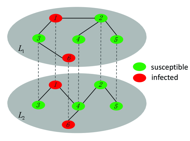
Figure 1: A schematic of our model. A susceptible node can be infected only if there are at least one infected neighbor in each layer, and an infected node can spontaneously recover to be susceptible. According to Eq.(2), node 3 can be infected by the common infected neighbor (node 1) with the rate $1.5\lambda$. But node 4 cannot be infected as (s)he has no infectious neighbors in the first layer.

We adopt a random sequential-update algorithm to simulate the model Chowdhury et al. (2005). We discretize the time in small time steps $\Delta t$. A node $i$ is first chosen randomly and is tried to update its state. If node $i$ is susceptible, (s)he becomes infected with the probability $R_{inf}\Delta t$. If node $i$ is infected, (s)he recovers to be susceptible with the probability $\mu\Delta t$. Time is then incremented by $\Delta t/N$ and we iterate up to some final time. The selection of $\Delta t$ is delicate. Too small $\Delta t$ will lead to the occurrence of null events very frequently, so that the simulation becomes inefficient. Too large $\Delta t$ will cause the updating probabilities larger than one that are unphysical. In practice, we used $\Delta t=1/(k_{max}\lambda)$ to minimize the probability that nothing happens while keeping all probabilities smaller than one, where $k_{max}$ is the maximal degree of nodes in two layers. Note that the random sequential-update algorithm has been widely used to simulate the continuous-time Markov process. It has also been verified that this algorithm did not produce essential difference from more sophisticated, but computationally demanding, exact Gillespie algorithm Gillespie (1977).

III Simulation Results

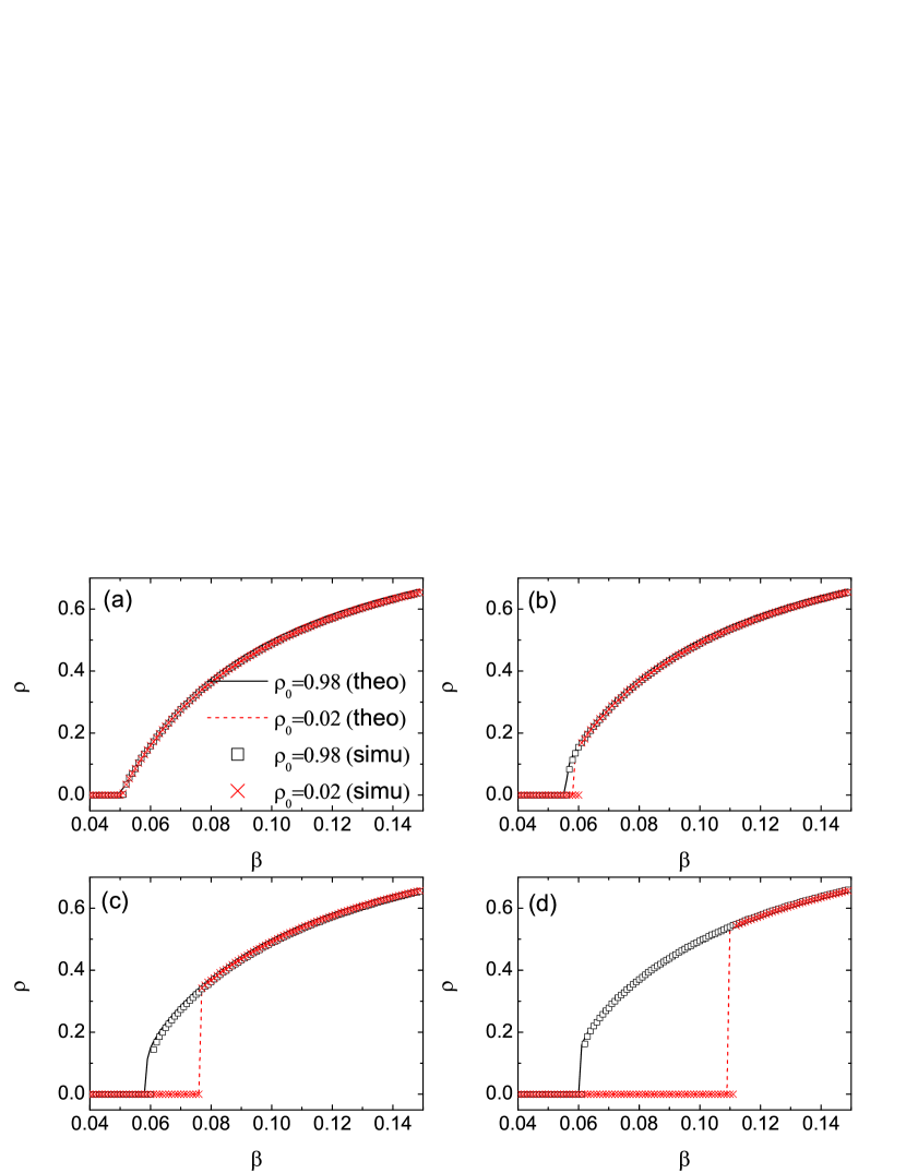
Figure 2: The density of infected nodes $\rho$ as a function of the infection rate $\beta$ in a two-layer network consisted of two Poisson random graphs. Two different initial infection densities are used: $\rho_{0}=0.98$ (squares) and $\rho_{0}=0.02$ (crosses). From (a) to (d) the overlap parameter $\mathcal{O}$ are 1.0, 0.8, 0.5, and 0.2, respectively. The other parameters are $N=10000$ and $\left\langle k\right\rangle=20$. The lines denote the results of homogeneous mean-field theory (see Eq.(26)).

We first consider the case where two layer networks are consisted of Poisson random graphs Erdös and Rényi (1959) with $N=10000$ nodes and the same average degree $\left\langle k\right\rangle=20$. Fig.2 shows the simulation results with two different initial infection density $\rho_{0}=0.02$ and $\rho_{0}=0.98$ and several different values of $\mathcal{O}$, where we have defined $\rho(t)=N^{-1}\sum\nolimits_{i=1}^{N}{\sigma_{i}(t)}$. For $\mathcal{O}=1$, our model recovers to the usual SIS model in single-layer networks, and the system undergoes a continuous second-order phase transition from a healthy phase to an endemic phase as $\beta$ increases, separated by a threshold value of $\beta_{c}$ (see Fig.2(a)). Strikingly, the nature of phase transition is essentially changed to be discontinuous for $\mathcal{O}<1$, as shown in Fig.2(b-d). The results for different initial conditions do not coincide in a certain range of $\beta\in\left[\beta_{F},\beta_{C}\right]$, forming a hysteresis region that is a typical characteristic of a first-order phase transition. Within the hysteresis region, the system is bistable. Specially, when the initial density of infection is low, the epidemic will become extinct. While for high initial density of infection, the system will maintain a certain proportion of prevalence. As $\mathcal{O}$ decreases, $\beta_{F}$ is almost unchanged and $\beta_{C}$ shifts to a larger value, thus the bistable region is enlarged.

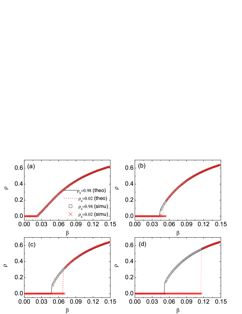
Figure 3: The density of infected nodes $\rho$ as a function of the infection rate $\beta$ in a two-layer network, in which the first layer is a BA network and the second one is obtained by rewiring edges from a BA network same as the first layer. Two different initial infection densities are used: $\rho_{0}=0.98$ (squares) and $\rho_{0}=0.02$ (crosses). From (a) to (d) the overlap parameter $\mathcal{O}$ are 1.0, 0.2, 0.1, and 0.0, respectively. The other parameters are $N=10000$ and $\left\langle k\right\rangle=20$. The lines denote the results of individual-based mean-field theory (see Eq.(21)).

In Fig.3, we show $\rho$ as a function of $\beta$ in a two-layer network, in which the first layer is a Barabási-Albert (BA) network Barabási and Albert (1999) and the second one is obtained by rewiring edges from a BA network same as the first layer. The qualitative results are the same as Fig.2. That is to say, for a more degree-heterogeneous network we also observe the discontinuous phase transition for the onset of epidemic outbreak and a bistable region with the coexisting healthy phase and endemic phase in a more degree-heterogeneous network. However, to observe such phenomena explicitly, we need to use lower degrees of overlap in edges among layers.

We now consider the case when the number of edges in the two layers are not the same. A particular example of interest is that one layer is completely embedded in another layer. This architecture will yield one layer completely overlapping with the second one but not the vice versa. In Fig. 4, we show the results in two Poisson random graphs with $N=10000$ nodes. The average degree in the first layer is fixed at 20, and the average degree in the second layer is twice (a) and four times (b) larger than that of the first layer. One can see that the phase transition is discontinuous. If the difference of connection densities between the two layers becomes larger, the discontinuous characteristic of the phase transition will become more obvious.

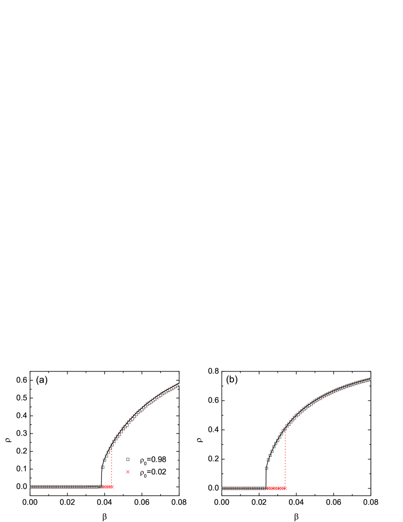
Figure 4: The density of infected nodes $\rho$ as a function of the infection rate $\beta$ in a two-layer Poisson random graph, in which the first layer is completely overlapped with the second one but not the vice versa. The average degree in the first layer is fixed at 20, and the average degree in the second layer is twice (a) and four times (b) larger than that of the first layer. Two different initial infection densities are used: $\rho_{0}=0.98$ (squares) and $\rho_{0}=0.02$ (crosses). The other parameter is $N=10000$. The lines denote the results of homogeneous mean-field theory (see Eq.(25)).

The key of the discontinuous phase transitions lies in the coexistence of two or more different stable phases. The origin of such a discontinuity in our model stems from the interaction between the nonlinearity of spreading dynamics introducing by Eq.(2) and the overlapping among the layers. For a multi-layer network with low overlap, an intuitive argument with regard to the coexistence of healthy phase and endemic phase may be presented as follows. For a high initial density of the infected nodes, most of nodes have at least one infected neighbor in each layer, such that the spread of epidemic is equivalent to that in single-layer network. When the initial density of the infected nodes is low, the reason why epidemics cannot spread is that most of nodes do not meet the condition of spreading dynamics in Eq.(2). That is to say, under the latter case, nonlinear effect of spreading dynamics does react and destroy connected infectious clusters, such that the epidemic dies out. This is akin to explosive synchronization in multiplex networks Jalan et al. (2019a, b), which demonstrate discontinuous transition in one layer due to suppression of formation of giant cluster drawn from the second layer, either due to frequency mismatch in the mirror nodes Jalan et al. (2019a) or due to negative intralayer coupling of the second layer Jalan et al. (2019b). In the next section, we will present a formulistic interpretation to the discontinuous phase transition based on a mean-field theory.

IV Mean-field theory

IV.1 individual-based mean-field theory

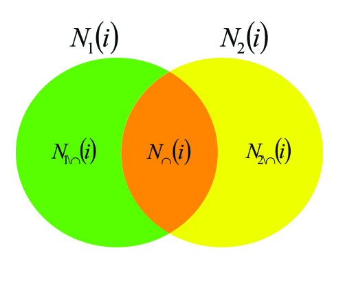
Figure 5: A schematic representation of neighborhood of node $i$. $N_{1}(i)$ and $N_{2}(i)$ denote the sets of neighbors of node $i$ in the first layer and in the second layer, respectively. $N_{\cap}(i)=N_{1}(i)\cap N_{2}(i)$ is the set of common neighbors of node $i$ in the two layers. $N_{1(2)\backslash{\cap}}(i)=N_{1(2)}(i)-N_{\cap}(i)$ is the set of neighbors of node $i$ belonging to the first (second) layer but not to the second (first) layer.

To be first, let $\rho_{i}(t)$ denote the probability of node $i$ being infected at time $t$. That is to say, at time $t$ the state of node $i$ takes the value $\sigma_{i}(t)=1$ with the probability $\rho_{i}(t)$ and $\sigma_{i}(t)=0$ with the complementary probability $1-\rho_{i}(t)$. To write down the time-evolution equation for node $i$, a key step is to derive the rate of node $i$ being infected at time $t$. To do so, we denote by $N_{1}(i)$ and $N_{2}(i)$ the set of neighbors of node $i$ in the first layer and in the second layer, respectively. Let $N_{\cap}(i)=N_{1}(i)\cap N_{2}(i)$ denote the set of common neighbors of node $i$ in the two layers, such that $N_{1(2)}(i)=N_{\cap}(i)+N_{1(2)\backslash{\cap}}(i)$, where $N_{1(2)\backslash{\cap}}(i)$ is the set of neighbors of node $i$ belonging to the first (second) layer but not to the second (first) layer, see Fig.5 for a schematic. The probability of having $\{n_{1},n_{2},n_{3}\}$ infected neighbors out of the sets $N_{1\backslash{\cap}}(i)$, $N_{{\cap}}(i)$, and $N_{2\backslash{\cap}}(i)$ can be repressed as the product of three Poisson binomial distributions,

$$P\left({{n_{1}},{n_{2}},{n_{3}}}\right)={P_{1}}\left({{n_{1}}}\right){P_{2}}\left({{n_{2}}}\right){P_{3}}\left({{n_{3}}}\right),$$ (3)

where

$${P_{1}}\left({{n_{1}}}\right)=\sum\limits_{Z\in{F_{1}}}{\prod\limits_{j\in Z}{{\rho_{j}}}}\prod\limits_{j\in{Z^{c}}}{\left({1-{\rho_{j}}}\right)}.$$ (4)

Here $F_{1}$ are all the subsets of $N_{1\backslash{\cap}}(i)$ containing $n_{1}$ elements, and $Z^{c}$ is the complement of $Z$, i.e., $Z^{c}=N_{1\backslash{\cap}}(i)\backslash Z$. Similarly, we can write down the expressions of $P_{2}(n_{2})$ and $P_{3}(n_{3})$ which are not shown here to avoid the duplication. According to Eq.(2), the rate of node $i$ being infected at time $t$ can be written as,

$${R_{\inf}}=\sum\limits_{{n_{1}}=0}^{\left|{{N_{1\backslash{\cap}}}}(i)\right|}{\sum\limits_{{n_{2}}=0}^{\left|{{N_{\cap}}}(i)\right|}{\sum\limits_{{n_{3}}=0}^{\left|{{N_{2\backslash{\cap}}}}(i)\right|}{P\left({{n_{1}},{n_{2}},{n_{3}}}\right)\lambda\left({\frac{{{n_{1}}+2{n_{2}}+{n_{3}}}}{2}}\right)\Theta\left({{n_{1}}+{n_{2}}-1}\right)\Theta\left({{n_{2}}+{n_{3}}-1}\right)}}},$$

(5)

where ${\left|{{N_{1\backslash{\cap}}}}(i)\right|}$, ${\left|{{N_{{\cap}}}}(i)\right|}$, and ${\left|{{N_{2\backslash{\cap}}}}(i)\right|}$ are the sizes of the sets of ${N_{1\backslash{\cap}}}(i)$, ${N_{{\cap}}}(i)$, and ${N_{2\backslash{\cap}}}(i)$, respectively. To facilitate the calculation of $R_{\inf}$, we rewrite Eq.(5) as,

$${R_{\inf}}= \sum\limits_{{n_{1}}=0}^{\left|{{N_{1\backslash{\cap}}}}(i)\right|}{\sum\limits_{{n_{2}}=0}^{\left|{{N_{\cap}}}(i)\right|}{\sum\limits_{{n_{3}}=0}^{\left|{{N_{2\backslash{\cap}}}}(i)\right|}{P\left({{n_{1}},{n_{2}},{n_{3}}}\right)\lambda\left({\frac{{{n_{1}}+2{n_{2}}+{n_{3}}}}{2}}\right)-}}}\sum\limits_{{n_{1}}=0}^{\left|{{N_{1\backslash{\cap}}}}(i)\right|}{P\left({{n_{1}},0,0}\right)\lambda\frac{{{n_{1}}}}{2}}$$ (6)

$$-\sum\limits_{{n_{3}}=0}^{\left|{{N_{2\backslash{\cap}}}}(i)\right|}{P\left({0,0,{n_{3}}}\right)\lambda\frac{{{n_{3}}}}{2}}.$$

The first term on the right hand side of Eq.(6) can be computed as,

$$\sum\limits_{{n_{1}}=0}^{\left|{{N_{1\backslash{\cap}}}}(i)\right|}{\sum\limits_{{n_{2}}=0}^{\left|{{N_{\cap}}}(i)\right|}{\sum\limits_{{n_{3}}=0}^{\left|{{N_{2\backslash{\cap}}}}(i)\right|}{P\left({{n_{1}},{n_{2}},{n_{3}}}\right)\lambda\left({\frac{{{n_{1}}+2{n_{2}}+{n_{3}}}}{2}}\right)}}}$$ (7)

$$= \frac{{\lambda}}{2}\left[{\sum\limits_{{n_{1}}=0}^{\left|{{N_{1\backslash{\cap}}}}(i)\right|}{{n_{1}}{P_{1}}\left({{n_{1}}}\right)+\sum\limits_{{n_{2}}=0}^{\left|{{N_{\cap}}}(i)\right|}{2{n_{2}}{P_{2}}\left({{n_{2}}}\right)+\sum\limits_{{n_{3}}=0}^{\left|{{N_{2\backslash{\cap}}}}(i)\right|}{{n_{3}}{P_{3}}\left({{n_{3}}}\right)}}}}\right]$$

$$= \frac{{\lambda}}{2}\left[{\left\langle{{n_{1}}}\right\rangle+2\left\langle{{n_{2}}}\right\rangle+\left\langle{{n_{3}}}\right\rangle}\right],$$

where

$$\begin{gathered}\left\langle{{n_{1}}}\right\rangle=\sum\limits_{j\in{N_{1\backslash{\cap}}}}{{\rho_{j}}}=\sum\limits_{j}{A_{ij}^{1}\left({1-A_{ij}^{2}}\right){\rho_{j}}},\hfill\\ \left\langle{{n_{2}}}\right\rangle=\sum\limits_{j\in{N_{\cap}}}{{\rho_{j}}}=\sum\limits_{j}{A_{ij}^{1}A_{ij}^{2}{\rho_{j}}},\hfill\\ \left\langle{{n_{3}}}\right\rangle=\sum\limits_{j\in{N_{2\backslash{\cap}}}}{{\rho_{j}}}=\sum\limits_{j}{A_{ij}^{2}\left({1-A_{ij}^{1}}\right){\rho_{j}}}.\hfill\\ \end{gathered}$$ (12)

The second term and the third term on the right hand side of Eq.(6) can be computed as,

$$\sum\limits_{{n_{1}}=0}^{\left|{{N_{1\backslash{\cap}}}}(i)\right|}{P\left({{n_{1}},0,0}\right)\lambda\frac{{{n_{1}}}}{2}=\frac{{\lambda}}{2}}{P_{2}}\left(0\right){P_{3}}\left(0\right)\sum\limits_{{n_{1}}=0}^{\left|{{N_{1\backslash{\cap}}}}(i)\right|}{{n_{1}}{P_{1}}\left({{n_{1}}}\right)=\frac{{\lambda}}{2}{P_{2}}\left(0\right){P_{3}}\left(0\right)\left\langle{{n_{1}}}\right\rangle},$$ (13)

and

$$\sum\limits_{{n_{3}}=0}^{\left|{{N_{2\backslash{\cap}}}}(i)\right|}{P\left({0,0,{n_{3}}}\right)\lambda\frac{{{n_{3}}}}{2}}=\frac{{\lambda}}{2}{P_{1}}\left(0\right){P_{2}}\left(0\right)\sum\limits_{{n_{3}}=0}^{\left|{{N_{2\backslash{\cap}}}}(i)\right|}{{n_{3}}{P_{3}}\left({{n_{3}}}\right)}=\frac{{\lambda}}{2}{P_{1}}\left(0\right){P_{2}}\left(0\right)\left\langle{{n_{3}}}\right\rangle,$$ (14)

respectively. Here

$$\begin{gathered}{P_{1}}\left(0\right){P_{2}}\left(0\right)=\prod\limits_{j\in{N_{1}(i)}}{\left({1-{\rho_{j}}}\right)}=\prod\limits_{j}{\left({1-A_{ij}^{1}{\rho_{j}}}\right)}\hfill,\\ {P_{2}}\left(0\right){P_{3}}\left(0\right)=\prod\limits_{j\in{N_{2}(i)}}{\left({1-{\rho_{j}}}\right)}=\prod\limits_{j}{\left({1-A_{ij}^{2}{\rho_{j}}}\right)}\hfill.\\ \end{gathered}$$ (18)

Substituting Eqs.(7,12,13,14,18) into Eq.(6), we have

$${R_{\inf}}= \frac{\lambda}{2}\sum\limits_{j}{\left({A_{ij}^{1}+A_{ij}^{2}}\right)}{\rho_{j}}-\frac{\lambda}{2}\prod\limits_{j}{\left({1-A_{ij}^{2}{\rho_{j}}}\right)}\sum\limits_{j}{A_{ij}^{1}\left({1-A_{ij}^{2}}\right){\rho_{j}}}$$ (19)

$$-\frac{\lambda}{2}\prod\limits_{j}{\left({1-A_{ij}^{1}{\rho_{j}}}\right)}\sum\limits_{j}{A_{ij}^{2}\left({1-A_{ij}^{1}}\right){\rho_{j}}}.$$

Thus, the time-evolution of $\rho_{i}$ can be written as

$$\begin{gathered}\frac{{d{\rho_{i}}}}{{dt}}=-\mu{\rho_{i}}+\left({1-{\rho_{i}}}\right){R_{\inf}}.\end{gathered}$$ (21)

Eq.(21) is the main theoretical result of the present work. It is not hard to check that $\rho_{i}=0$ ($i=1,\cdots,N$) is always a set of stationary solution of Eq.(21). Near the onset of epidemic outbreak, $\rho_{i}\simeq 0$, Eq.(21) can be linearized as,

$$\frac{{d{\rho_{i}}}}{{dt}}=-\mu{\rho_{i}}+\lambda\sum\limits_{j}{A_{ij}^{1}A_{ij}^{2}}{\rho_{j}},$$ (22)

or in the matrix form,

$$\frac{{d\vec{\rho}}}{{dt}}=\left({-\mu\textbf{I}+\lambda\tilde{\textbf{A}}}\right)\vec{\rho},$$ (23)

where $\vec{\rho}={\left[{{\rho_{1}},\ldots,{\rho_{N}}}\right]^{T}}$, I is the $N$-dimensional identity matrix, and the entries of $\tilde{\textbf{A}}$ are $\tilde{A}_{ij}={A_{ij}^{1}A_{ij}^{2}}$. That is to say, $\tilde{A}_{ij}=1$ only when $A_{ij}^{1}=1$ and $A_{ij}^{2}=1$ simultaneously, and therefore we call $\tilde{\textbf{A}}$ the overlapping adjacency matrix of multiplex network. The solution $\rho_{i}=0$ loses its stability when the largest eigenvalue of $-\mu\textbf{I}+\lambda\tilde{\textbf{A}}$ is larger than zero, which determines the epidemic threshold that is the reciprocal of the largest eigenvalue of $\tilde{\textbf{A}}$, i.e.,

$${\beta_{C}}=\frac{1}{{{\Lambda_{\max}}\left({\tilde{\textbf{A}}}\right)}}.$$ (24)

For $\mathcal{O}=1$, Eq.(24) recovers to the result of single-layer networks Y. Wang ; Mieghem et al. (2009); Gómez et al. (2010), $\beta_{C}(\mathcal{O}=1)=1/\Lambda_{max}(\textbf{A})$. For $\mathcal{O}=0$, $\tilde{\textbf{A}}$ becomes a null matrix and therefore $\beta_{C}(\mathcal{O}=0)=\infty$. For $0<\mathcal{O}<1$, $\beta_{C}$ falls between $\beta_{C}(\mathcal{O}=1)$ and $\beta_{C}(\mathcal{O}=0)$.

In Fig.6, we show the phase diagram of the model in $\beta\sim\mathcal{O}$ space. We use the same networks as the Fig.3. The phase diagram is divided into three regions, separated by two transition values of $\beta$, $\beta_{F}$ and $\beta_{C}$. $\beta_{C}$ is obtained by calculating the largest eigenvalue of the overlapping adjacency matrix (see Eq.(24)). Note that due to nonlinear characteristic of Eq.(21) $\beta_{F}$ cannot be obtained in general by analytical derivation. Alternatively, $\beta_{F}$ is obtained by numerically solving the steady equation of $\rho_{i}$ (letting $d\rho_{i}/dt=0$ in Eq.(21)) using the initial condition $\rho_{i}(0)=1$.

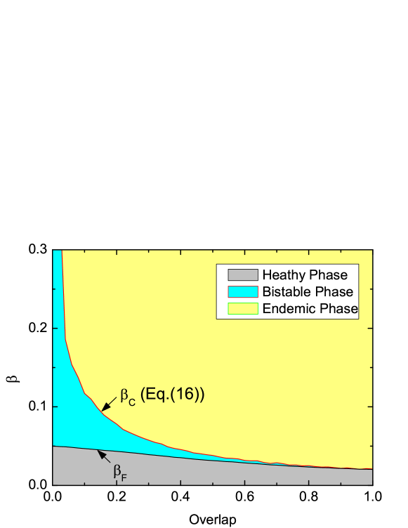
Figure 6: Phase diagram in $\beta\sim\mathcal{O}$ plane. The used networks are the same as those in Fig.3.

IV.2 homogeneous mean-field theory

For homogeneous networks, each node is assumed to be statistically equivalent, and thus $\rho_{i}=\rho$ for $\forall i$, and degrees of each node in each layer are the same, i.e., $\sum\nolimits_{j}{A_{ij}^{1}}=\left\langle k\right\rangle_{1}$ and $\sum\nolimits_{j}{A_{ij}^{2}}=\left\langle k\right\rangle_{2}$ for $\forall i$. Here, the rate equation for homogeneous mean-field theory does not need to be rederived. Alternatively, it can be obtained by rewriting Eq.(21) based on the above assumption in homogeneous networks. Thus, $\sum\nolimits_{j}{A_{ij}^{1(2)}}{\rho_{j}}=\left\langle k\right\rangle_{1(2)}\rho$, $\prod\nolimits_{j}\left(1-A_{ij}^{1(2)}{\rho_{j}}\right)=\left({1-\rho}\right)^{\left\langle k\right\rangle_{1(2)}}$, and $\sum\nolimits_{j}A_{ij}^{1(2)}\left({1-A_{ij}^{2(1)}}\right){\rho_{j}}=\left\langle k\right\rangle_{1(2)}\left({1-\mathcal{O}_{1(2)}}\right)\rho$, and Eq.(21) can be rewritten as,

$$\frac{{d\rho}}{{dt}}=-\mu\rho+\frac{\lambda}{2}\rho\left({1-\rho}\right)\left[{{{\left\langle k\right\rangle}_{1}}+{{\left\langle k\right\rangle}_{2}}-{{\left\langle k\right\rangle}_{1}}{{\left({1-\rho}\right)}^{{{\left\langle k\right\rangle}_{2}}}}\left({1-{\mathcal{O}_{1}}}\right)-{{\left\langle k\right\rangle}_{2}}{{\left({1-\rho}\right)}^{{{\left\langle k\right\rangle}_{1}}}}\left({1-{\mathcal{O}_{2}}}\right)}\right],$$

(25)

where we have defined $\mathcal{O}_{1(2)}=\sum\nolimits_{i<j}{A_{ij}^{1}}A_{ij}^{2}/\sum\nolimits_{i<j}{A_{ij}^{1(2)}}$ as the fraction of the number of overlapping edges in the total number of edges in the first (second) layer. When the numbers of edges in each layer are the same as considered before, $\mathcal{O}_{1}=\mathcal{O}_{2}=\mathcal{O}$, $\left\langle k\right\rangle_{1}=\left\langle k\right\rangle_{2}=\left\langle k\right\rangle$, Eq.(25) can be simplified to

$$\frac{{d\rho}}{{dt}}=-\mu\rho+\lambda\left\langle k\right\rangle\left({1-\rho}\right)\rho\left[{1-\left({1-\mathcal{O}}\right){{\left({1-\rho}\right)}^{\left\langle k\right\rangle}}}\right].$$ (26)

Notice that $\rho=0$ is always a stationary solution of Eq.(26). Such a trivial solution corresponds to the healthy phase where no infected nodes survive. According to linear stability analysis, the solution becomes unstable when the derivative of the right hand side of Eq.(26) with respect to $\rho$ at $\rho=0$ is larger than zero, which determines the epidemic threshold $\beta_{C}$,

$${\beta_{C}}=\frac{1}{{\left\langle k\right\rangle\mathcal{O}}}.$$ (27)

Comparing to mean-field equation of the SIS model in single-layer networks Pastor-Satorras et al. (2015), our model can give rise to an additional term in Eq.(26), ${\left({1-\mathcal{O}}\right){{\left({1-\rho}\right)}^{\left\langle k\right\rangle}}}$. Obviously, the additional term vanishes in the case of $\mathcal{O}=1$. Importantly, we shall see that for $\mathcal{O}\neq 1$ the additional term can lead to an essential change in the bifurcation of the model. The results for the simple mean-field theory are summarized in Fig.7. Fig.7(a-c) shows $\rho$ as a function of $\beta$ for three distinct values of $\mathcal{O}$. For $\mathcal{O}=1$, our model recovers to the standard SIS model, and it is well-known that $\rho$ shows a transcritical bifurcation as $\beta$ varies. Across the epidemic threshold $\beta=1/\left\langle k\right\rangle$ (here we have used $\left\langle k\right\rangle=20$) from below, the trivial solution $\rho=0$ loses its stability, and a new solution of $\rho\neq 0$ arises. In physics, we call that the model undergoes a continuous phase transition from a healthy phase ($\rho=0$) to an endemic phase ($\rho>0$) at $\beta=\beta_{C}$. For $\mathcal{O}\neq 1$, the bifurcation feature is changed essentially. When $\beta<\beta_{F}$, $\rho=0$ is only stable solution. When $\beta_{F}<\beta<\beta_{C}$, there exist two stable solutions, $\rho=0$ and $\rho>0$, and an unstable solution ($\rho^{uns}$) lying in between the two stable solutions. Depending on the initial density $\rho_{0}$ of infected nodes, the system will arrive at either a healthy phase (for $\rho_{0}<\rho^{uns}$) or an endemic phase (for $\rho_{0}>\rho^{uns}$). As $\beta$ approaches $\beta_{F}$ or $\beta_{C}$, one of stable solutions and the unstable solution of $\rho$ get close to each other, until they colloid and annihilate via a saddle-node bifurcation. When $\beta>\beta_{C}$, $\rho=0$ is unstable and $\rho>0$ is only stable. Therefore, for $\mathcal{O}<1$ the system is divided into three phases in terms of $\beta$. For $\beta<\beta_{F}$ the system is in the healthy phase. For $\beta>\beta_{C}$ the system is in the endemic phase. Between them, the system is in bistable phase. Fig.7(d) shows the phase diagram in the parametric space $\beta\sim\mathcal{O}$. The boundary line $\beta_{F}$ shows a very slow decrease as $\mathcal{O}$ increase, and the other one $\beta_{C}$ decreases obviously with $\mathcal{O}$ according to Eq.(27), such that we can see that the bistable region is clearly enlarged as $\mathcal{O}$ decreases.

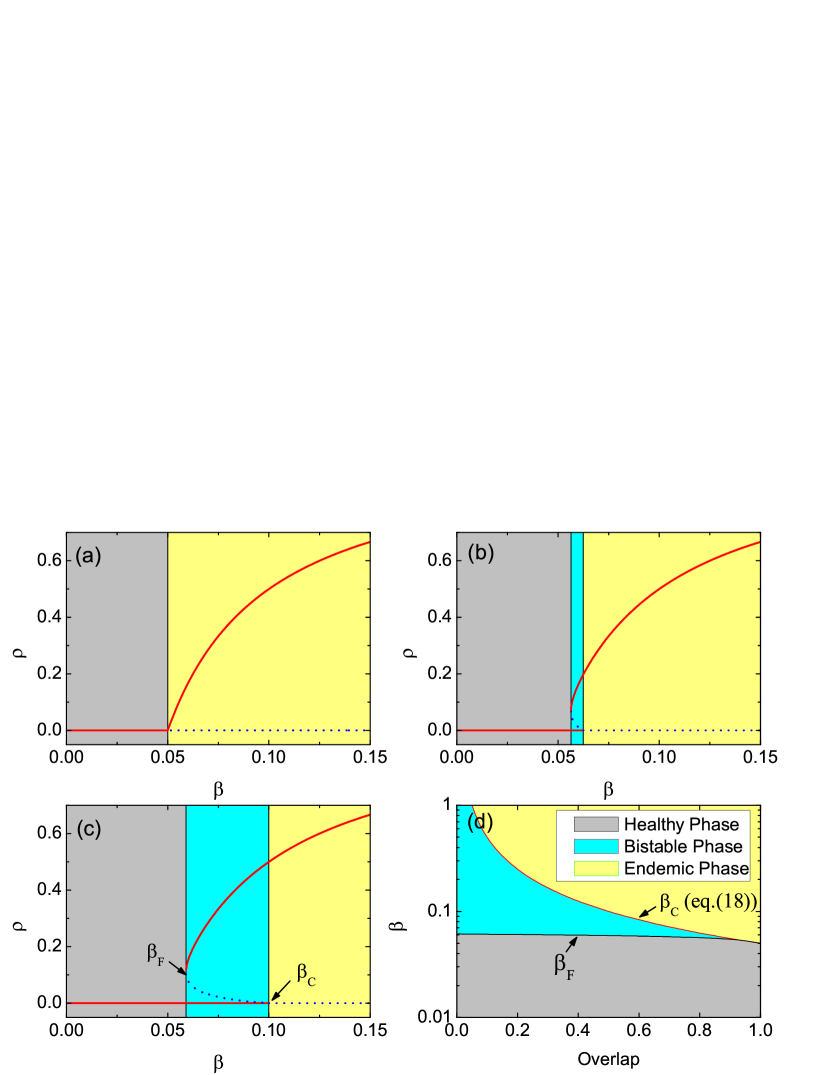
Figure 7: Results from the homogeneous mean-field theory. (a-c) shows $\rho$ versus $\beta$ for three different $\mathcal{O}$: 1.0 (a), 0.8(b), and 0.5 (c). (d) shows the phase diagram in $\beta\sim\mathcal{O}$ plane. Solid lines and dotted lines in (a-c) denote stable and unstable solutions, respectively. The average degree is $\left\langle k\right\rangle=20$.

V Comparison between simulation and theory

It is expected that the homogenous mean-field theory coincides with the simulation results in Poisson random graph (shown in Fig.2). To compare them, we numerically solve Eq.(26) using the same initial conditions as the simulations, and theoretical results are shown by lines in Fig.2. There are an excellent agreement between the theory and simulation. We should note that the theoretical value of $\beta_{C}$ is not easy to access in simulation. For example, for $\left\langle k\right\rangle=20$ and $\mathcal{O}=0.5$, we have $\beta_{C}=0.1$ in terms of Eq.(27) (shown in Fig.7(c)). In simulation, we use $\rho_{0}=0.02$ and give $\beta_{C}=0.076$, as shown in Fig.2(c). In principle, we can access the theoretical limit of Eq.(27) by using a lower initial density of infection in simulation. However, if the number of infected seeds is very small, the finite-size fluctuations may drive, with a very high probability, the system to the absorbing state whenever no more infected nodes survive. Once the absorbing state is reached, the system cannot be left. Therefore, in order to verify the theoretical prediction in Eq.(27) with an adequate accuracy, one needs to use a considerable large network size to reduce the finite-size fluctuations. It will certainly increase more computational resource.

For more degree heterogeneous networks, individual-based mean-field theory is more appropriate. Using the duplex networks same as those in Fig.3, we numerically solve Eq.(21) to obtain stationary value of $\rho_{i}$ and the average infection density $\rho=N^{-1}\sum\nolimits_{i=1}^{N}{\rho_{i}}$, as indicated by lines in Fig.3. As expected, the theory can well reproduce the simulation results.

VI Results on other multiplex networks

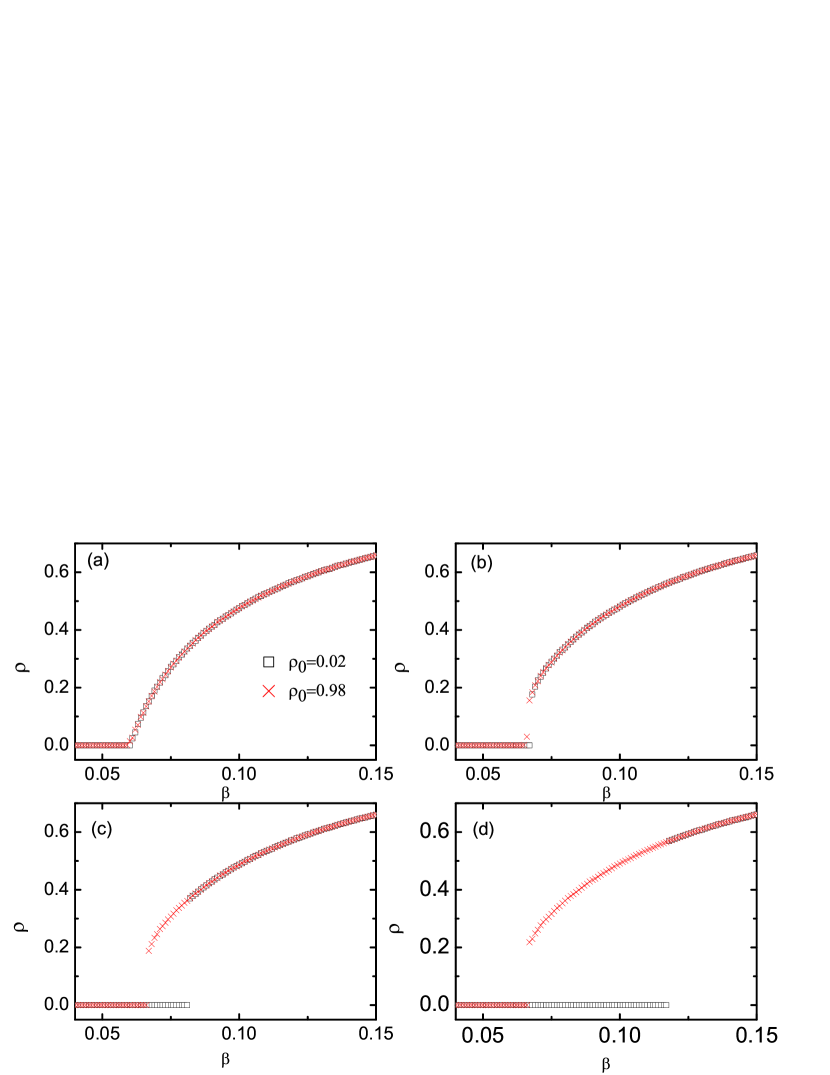
Figure 8: The density of infected nodes $\rho$ as a function of the infection rate $\beta$ in a two-layer network where the first layer is consisted of a Watts-Strogatz small-world network and the second layer is obtained by randomly rewiring the first layer network such that a given fraction of overlapping edges is achieved. Two different initial infected densities are used: $\rho_{0}=0.02$ (squares) and $\rho_{0}=0.98$ (crosses). From (a) to (d) the overlap parameters $\mathcal{O}$ are 1.0, 0.8, 0.5, and 0.2, respectively. The other parameters are $N=10000$ and $\left\langle k\right\rangle=20$.

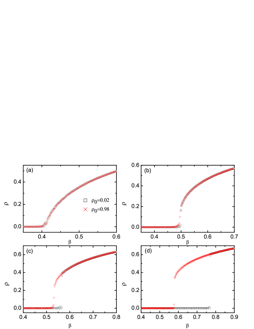
Figure 9: The density of infected nodes $\rho$ as a function of the infection rate $\beta$ in a two-layer network where the first layer is consisted of a $100\times 100$ square lattice and the second layer is obtained by randomly rewiring the first layer network such that a given fraction of overlapping edges is achieved. Two different initial infected densities are used: $\rho_{0}=0.02$ (squares) and $\rho_{0}=0.98$ (crosses). From (a) to (d) the overlap parameters $\mathcal{O}$ are 1.0, 0.8, 0.7, and 0.5, respectively.

To validate the generality of our conclusion, we also present the simulation results in other multiplex networks. In Fig.7, the first layer is consisted a Watts-Strogatz small-world network Watts and Strogatz (1998). The small-world network is generated as follows. We start with a regular ring network with $N=10000$ nodes in which each node is connected to its first $K=20$ neighbors ($K/2$ on either side), and we then randomly rewire each edge of the ring network with probability $p=0.05$ such that $pNK/2$ long-range edges are generated. In Fig.8, the first layer is consisted of a $100\times 100$ square lattice (periodic boundary) in which each node is connected to its four nearest neighbors. The second layers both in Fig.7 and Fig.8 are obtained by randomly rewiring the first layer network such that a given fraction of overlapping edges is achieved. From Fig.7 and Fig.8, one sees that for less degrees of overlapping edges in the two layers, a discontinuous phase transition can be also observed. That is to say, the main conclusion in our work holds for other network models as well.

In Fig.9, we show the results on a three-layer network consisted of three Poisson random graphs with $N=10000$ and $\left\langle k\right\rangle=20$, in which we have assumed that a susceptible node can be infected only when it has at least one infectious neighbor in each layer. It can be seen that the main conclusions are consistent with those in a two-layer network. At last, we perform simulations on two real multiplex networks: C.Elegans multiplex connectome Chen et al. (2006); De Domenico et al. (2015a) and SACCHCERE multiplex network Stark et al. (2006); De Domenico et al. (2015b). We find that they can produce discontinuous phase transition as well, as shown in Fig.10.

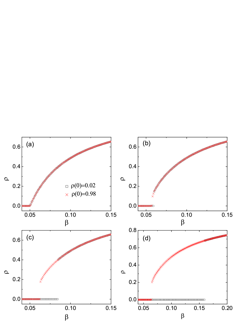
Figure 10: The density of infected nodes $\rho$ as a function of the infection rate $\beta$ in a three-layer network consisted of three Poisson random graphs. Two different initial infection densities are used: $\rho_{0}=0.02$ (squares) and $\rho_{0}=0.98$ (crosses). From (a) to (d) the overlap parameter $\mathcal{O}$ are 1.0, 0.8, 0.5, and 0.2, respectively. The other parameters are $N=10000$ and $\left\langle k\right\rangle=20$.

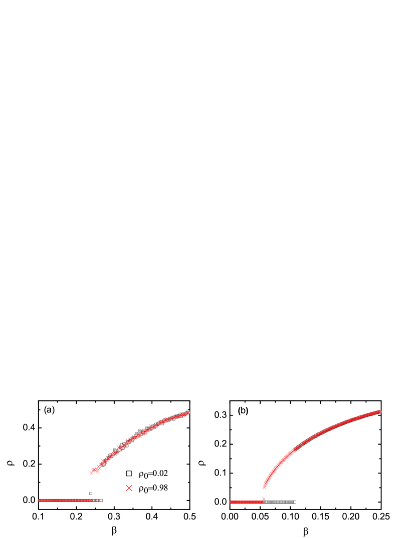
Figure 11: The density of infected nodes $\rho$ as a function of the infection rate $\beta$ in two real multiplex networks. Two different initial infection densities are used: $\rho_{0}=0.02$ (squares) and $\rho_{0}=0.98$ (crosses). (a) C.Elegans multiplex connectome consisted of three layers corresponding to different synaptic junctions: electric, chemical monadic, and chemical polyadic Chen et al. (2006); De Domenico et al. (2015a). The multiplex network contains 279 nodes and 5863 edges . The overlap parameter is $\mathcal{O}=0.165$. (b) SACCHCERE multiplex network Stark et al. (2006); De Domenico et al. (2015b). The original network is consisted of seven layers, but we only used the first four layers: physical association, suppressive genetic interaction defined by inequality, direct interaction, and synthetic genetic interaction defined by inequality. The multiplex network contains 6570 nodes and 151991 edges. The overlap parameter is $\mathcal{O}=0.013$. Note here that the number of edges in each layer is not the same, and the overlap parameter $\mathcal{O}$ is defined as the number of overlapping edges in all layers divided by the minimum of the number of edges in all layers.

VII Conclusions

In conclusion, we have studied an SIS-type epidemic spreading model in multiplex networks, in which a susceptible individual can be infected only when (s)he has at least one infectious neighbor in each layer. We find that the proportion of overlapping edges between different layers has a significant impact on the nature of phase transition for the epidemic outbreak. When all the edges are completely overlapped, the model recovers to the standard SIS model in single-layer networks, and it undergoes a continuous phase transition. Otherwise, the model shows an essentially different nature of phase transition, that is of a discontinuous first order. Using low and high initial densities of infected individuals, the model shows two distinct transition pathways from an endemic extinction phase to an endemic spread phase as the infection rate increases. Such two pathways form a hysteresis region in which the system is bistable with the coexisting endemic extinction phase and endemic spread phase. As the degree of overlapping edges decreases, the left boundary of the hysteresis region changes slowly, but the right boundary of the hysteresis region moves swiftly to a larger value of the infection rate, such that the hysteresis region is enlarged as $\mathcal{O}$ decreases. Moreover, we have developed an individual-based mean-field theory that can derive the time-evolution equations of infected probabilities of individuals. The individual-based mean-field equations can be reduced to a single equation of average infection density. Such a coarse graining is advantageous to unveil the physical mechanics of phenomena observed in simulations. By linear stability analysis, we have derived the threshold of epidemic outbreak, corresponding to the right boundary of hysteresis region. Our theory can well reproduce the simulation results.

Recently, there were some studies that reported distinct mechanisms leading to discontinuous or explosive spreading outbreak in single-layer networks, such as reinfections in social contagions Gómez-Gardeñes et al. (2015), synergistic effect in transmission rate Gómez-Gardeñes et al. (2016), cooperative coinfections of multiple diseases Chen et al. (2013); Cai et al. (2015); Hébert-Dufresnea and Althousea (2015), core contact process Chae et al. (2015); Varghese and Durrett (2013), and higher-order interactions between individuals Iacopini et al. (2019), etc. The present work shows a new mechanism that can lead to a discontinuous phase transition due to the interacting spreading dynamics across different network layers. This mechanism underlies the importance of correlations in edges belong to different layers. Therefore, our study adds to the continuing effort of the effects of multiplexity on dynamic processes on multiplex networks, compared to conventional single-layer ones. On the one hand, in most social systems, individuals interact with each other in complicated patterns that include multiple types of relationships. The present findings may improve our understanding for some real-world spreading processes in such complex systems such as the spread of a rumor, the formation of a new opinion. On the other hand, a common characteristic of discontinuous epidemic outbreak is that infinitesimal increase of the external parameters, such as infection rate, can give rise to a considerable macroscopic spreading scope. There is no doubt that it brings more challenges for controlling or predicting epidemic outbreaks D’Souza et al. (2019). Finally, we expect that the present theoretical findings can be supported by empirical or experimental research in the future.