Exploring BSM Higgs couplings in single top-quark production

Abstract

In this article we study a Standard Model extension modifying the top-quark Yukawa coupling to the Higgs boson by allowing a mixture of CP-odd and -even couplings. Single top-quark production in association with an additional Higgs boson provides a natural laboratory to search for such extensions. However, because of the small cross section the experimental analysis is challenging. Already the measurement of the cross section for this process is highly non-trivial. Furthermore, using only cross section measurements, a certain parameter region would escape detection. Using an explicit BSM scenario we show that employing the Matrix Element Method a precise measurement becomes feasible. Ignoring signal detection efficiencies an integrated luminosity of about $20$ fb^-1 would allow a discovery. Assuming signal detection efficiencies at the level of a few percent a potential signal could be established in the high luminosity phase of the LHC.

I Introduction

The discovery of the Higgs boson by the ATLAS and CMS collaborations Aad:2012tfa ; Chatrchyan:2012xdj in 2012 completed the Standard Model. In many subsequent measurements the Higgs boson properties were studied, analysing a variety of different Higgs boson production and decay processes. Even though no deviations from the Standard Model predictions have been reported by the experiments so far, there is a great interest in further studies of the Higgs Yukawa sector as this is a crucial part of the Higgs mechanism—the Standard Model mechanism to spontaneously break the electroweak symmetry. In particular, since in many beyond the Standard Model (BSM) scenarios the Higgs sector is modified. Prominent examples are for instance, the two-Higgs-doublet model (2HDM) Branco:2011iw and composite Higgs models Agashe:2004rs which both predict modified Higgs couplings and introduce CP-violating Yukawa interactions.

In the Higgs sector of the Standard Model the top quark plays a special role because of its large Yukawa coupling $(y_{t}=\sqrt{2}~{}m_{t}/v\sim 1)$. Thus, if physics beyond the Standard Model modifies the Higgs sector, deviations are expected to be seen first in the top-Higgs interaction. This makes precise studies of the top-Higgs dynamics a promising laboratory to search for new physics.

In fact, not only the value of the top-quark Yukawa coupling is of high interest but also its relative sign with respect to the Higgs boson interactions with gauge bosons. A relative sign between these couplings different from the Standard Model prediction, has a severe impact on the electroweak symmetry breaking mechanism and leads to a violation of unitarity Appelquist:1987cf . As a further test of the Standard Model, it is thus important to analyse the top-Higgs coupling in more detail. Such studies can also provide a further consistency test of the CP properties of the Higgs boson.

At the LHC, the top-quark Yukawa coupling is experimentally accessible only in a few processes. It can be inferred indirectly in the dominant Higgs boson production process via gluon fusion, where the Higgs couples to a closed top-quark loop. Recently, also an indirect measurement of the top-quark Yukawa coupling from electroweak corrections to top-quark pair production Sirunyan:2019nlw has been presented. Common to all indirect measurements is that the extraction of the Yukawa coupling can be spoiled by unaccounted BSM effects. In contrast, the production of a Higgs boson in association with top quarks allows a direct measurement of the corresponding interaction. The recent discovery of the $t\bar{t}H$ process at the LHC Sirunyan:2018hoz ; Aaboud:2018urx allows for the first time a direct determination of the interaction strength. However, neglecting the masses of the light quarks, the $t\bar{t}H$ cross section is insensitive to the sign of the top-quark Yukawa coupling because of its quadratic dependence.

Complementary information can be gathered from Higgs boson production in association with a single top quark. In particular, this process offers the rather unique opportunity to study the relative sign between the top-quark Yukawa and the Higgs-gauge boson interaction terms.

Figure 1: Leading order Feynman diagrams for $pp\to tH$ in the $t$-channel production process.

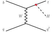
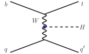
Within the Standard Model (SM) the dominant production mode at the LHC is via the $t$-channel exchange of a $W$ boson, as illustrated in Fig. 1. The Higgs boson can be emitted either from the top quark or from the virtual $W$ boson. In the Standard Model each individual contribution is sizeable. However, the total cross section is reduced by a significant destructive interference between the two diagrams, which originates from the cancellation of the longitudinal $W$ boson polarization Bordes:1992jy ; Maltoni:2001hu ; Farina:2012xp . Thus, besides the prominent example of longitudinal $W$-boson scattering, single top-quark production in association with a Higgs boson also serves as a testing ground for the unitarisation of the Standard Model as realised by the Higgs mechanism.

Based on these unique opportunities the process has received a lot of attention in recent years Bordes:1992jy ; Maltoni:2001hu ; Farina:2012xp ; Biswas:2012bd ; Agrawal:2012ga ; Taghavi:2013wy ; Campbell:2013yla ; Ellis:2013yxa ; Chang:2014rfa ; Kobakhidze:2014gqa ; Wu:2014dba ; Englert:2014pja ; Demartin:2015uha ; Gritsan:2016hjl ; Rindani:2016scj ; Barger:2018tqn ; Degrande:2018fog even though the experiments have only presented searches for this production channel Khachatryan:2015ota ; Sirunyan:2018lzm so far. The reason is that the experimental signature is very challenging and the total cross section is very small, requiring sophisticated analysis techniques to become sensitive to this reaction.

In this article, we extend previous studies and use the Matrix Element Method Kondo:1988yd ; Kondo:1991dw to extract the top-quark Yukawa coupling. In recent years, the Matrix Element Method has been established as a powerful method to extract information in cases where one suffers from small event rates and complicated backgrounds. As a concrete example we investigate the Standard Model extension studied in Ref. Artoisenet:2013puc . This model introduces a CP-violating top-quark Yukawa coupling keeping at the same time the top-quark mass fixed. It is thus possible to parametrise potential deviations from the Standard Model in a continuous way. Alternatively, one could also study a two-Higgs-doublet model as a specific example.

We give first some details on the computation and illustrate the impact of the new coupling at the inclusive level. In addition, a brief review of the general idea of the Matrix Element Method is presented. Finally, we discuss the potential constraining power of the method in the context of the $pp\to tH$ production process and conclude.

II CP-violating Yukawa coupling

In order to study the top-quark Yukawa coupling independently of the top-quark mass we follow Ref. Artoisenet:2013puc and allow for a mixture of CP-even and CP-odd interactions. In this scenario the parametrization of the interaction vertex of the top quark and the Higgs boson is given by Artoisenet:2013puc

$$\mathcal{L}_{t\bar{t}H}=-\frac{y_{t}}{\sqrt{2}}\left(a\cos(\alpha)\bar{t}t+ib\sin(\alpha)\bar{t}\gamma_{5}t\right)H.$$ (1)

In addition, we use for the parameters $a$ and $b$ the setting of Ref. Demartin:2015uha :

$$a=1,\qquad b=\frac{2}{3},$$ (2)

to keep the $gg\to H$ total cross section unmodified for any value of $\alpha$. Thus, the model has only one free parameter, namely the CP-mixing angle $\alpha$. Varying $\alpha$ allows to interpolate continuously between the CP-even $(\alpha=0^{\circ})$ and the CP-odd $(\alpha=180^{\circ})$ scenario.

In the following, we study the impact of the modified coupling on the dominant $t$-channel production of a single top quark in association with a Higgs boson at the next-to-leading order (NLO) in QCD. The analysis is performed for the LHC Run II energy of $\sqrt{s}=13$ TeV. The following Standard Model input parameters are used

$$m_{t}=173.2~{}\textrm{GeV},\quad m_{W}=80.385~{}\textrm{GeV},\quad m_{H}=125~{}\textrm{GeV}.$$

We require that the hardest light jet, as well as the top-tagged jet and the Higgs boson, fulfill the following selection cuts

$$p_{T}(X)>30~{}\textrm{GeV}\;,\quad|\eta(X)|<3.5\;,\quad X\in\{t,H,j\}\;,$$

where jets are defined using the $k_{T}$-jet algorithm Cacciari:2011ma with a jet radius parameter of $R=0.4$. In addition, we require that all final state objects are well separated with $\Delta R_{ij}>0.4$.The renormalisation and factorisation scales are set to the common value of $\mu_{R}=\mu_{F}=m_{t}$. We have cross-checked the calculation at the differential level with results obtained from aMC@NLO Alwall:2014hca ; Artoisenet:2013puc .

Figure 2: The fiducial cross section of $pp\to tH$ as a function of the CP-mixing angle $\alpha$ at LO and NLO accuracy.

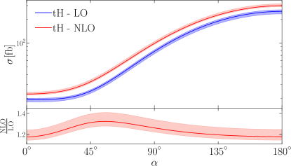
In Fig. 2 the fiducial cross section as a function of the CP-mixing angle $\alpha$ is shown. The upper panel depicts the predictions for LO and NLO together with the theoretical uncertainties obtained by varying the factorisation and renormalisation scale by a factor of two up and down. The bottom panel illustrates the relative size of the NLO corrections with respect to the LO predictions. The central prediction for the fiducial cross section at the next-to-leading order in QCD as a function of the CP-mixing angle $\alpha$ can be parametrised for the aforementioned setup by

$$\sigma_{\textrm{fid}}^{\textrm{NLO}}(\alpha)=\sigma_{\textrm{fid}}^{\textrm{SM}}~{}\big{[}4.37-6.10\cos(\alpha)+2.73\cos^{2}(\alpha)\\ -0.01\sin(\alpha)+0.00\cos(\alpha)\sin(\alpha)\big{]}\;,$$ (3)

with $\sigma_{\textrm{fid}}^{\textrm{SM}}=22.6$ fb. The tiny value of the $\sin(\alpha)$ contribution and the compatibility of the $\cos(\alpha)\sin(\alpha)$ coefficient with zero (within its numerical uncertainty) are a consequence of the applied phase-space cuts, which constrain the preferred phase-space region of the pseudoscalar contribution Demartin:2015uha . We want to stress that the smallness of the $\sin(\alpha)$ and $\cos(\alpha)\sin(\alpha)$ coefficients does not mean that the CP-odd contributions are negligible. In fact, contributions of the form $\sin^{2}(\alpha)$ are distributed across the constant and the $\cos^{2}(\alpha)$ coefficients. For completeness we also provide the total inclusive cross section at the next-to-leading order in QCD

$$\sigma_{\textrm{tot}}^{\textrm{NLO}}(\alpha)=\sigma_{\textrm{tot}}^{\textrm{SM}}~{}\big{[}4.70-5.19\cos(\alpha)+1.49\cos^{2}(\alpha)\\ -0.95\sin(\alpha)+0.59\cos(\alpha)\sin(\alpha)\big{]}\;,$$ (4)

with $\sigma_{\textrm{tot}}^{\textrm{SM}}=46.7$ fb. Notice that due to the coupling structure given by Eqn. (1) a similar decomposition holds for all observables for this process as long as only QCD corrections are taken into account.

Inspecting Fig. 2, one observes that the NLO corrections are positive and sizeable over the whole range. The Standard Model prediction as well as the ‘inverted’ SM $(\alpha=180^{\circ})$ receive corrections up to $+18\%$, while for $\alpha\approx 56^{\circ}$ the corrections can reach up to $+32\%$. Note, that the maximum of the NLO corrections happens to coincide with the maximal mixing of the CP-even and CP-odd coupling, which is different from $\alpha=45^{\circ}$ due to the choice $a\neq b$ in Eqn. (1). As one would naively expect, the theoretical uncertainty, as estimated by scale variation, is rather constant over the whole range and amounts to $+6\%$ and $-3\%$. The fact that the NLO prediction lies outside of the LO uncertainty band underlines the importance of the NLO calculation. The non-overlapping uncertainty bands are not surprising since in leading order the process $pp\to tH$ is of pure electroweak nature. Thus, it is mandatory to include NLO corrections since they are large and depend on the CP-mixing angle $\alpha$.

Figure 3: Zoom of Fig. 2. The dashed lines illustrate the interval in $\alpha$ that is still compatible with the SM prediction within its uncertainties.

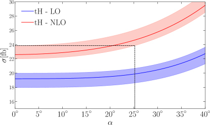
Zooming into the region of small $\alpha$ (c.f. Fig. 3), one can see that using only the information of the inclusive cross section a significant interval of $\alpha$ cannot be distinguished from the Standard Model case ($\alpha=0^{\circ}$). In fact, by taking the scale uncertainty into account, the cross sections obtained for $0^{\circ}\leq\alpha\leq 25.2^{\circ}$ are compatible with the Standard Model prediction.

A more precise determination of the CP-mixing angle $\alpha$ is expected from shape differences of differential distributions. However, using standard cut-based techniques this requires a sufficient amount of recorded events which will only become available in the far future. Another drawback of differential distributions is that detailed studies Demartin:2015uha are necessary in order to isolate specific observables that show a good sensitivity on the parameter under scrutiny. If on the other hand several observables are used at the same time, possible correlations, which can be difficult to quantify, need to be taken into account. In order to get the full benefit of currently available data, we propose to use the Matrix Element Method. In the next section, we give a brief introduction before applying the method to the concrete case.

III The Matrix Element Method

The Matrix Element Method (MEM) was first introduced in Refs. Kondo:1988yd ; Kondo:1991dw to separate signal from background processes. However, the method is rather general and can also be used to determine parameters of the underlying theory. While the formulation of the MEM has been restricted to LO accuracy for a long time, the inclusion of NLO QCD effects has been expedited within the last decade Alwall:2010cq ; Campbell:2012cz ; Baumeister:2016maz and has recently been achieved in a generic way Martini:2015fsa ; Martini:2017ydu ; Martini:2018imv ; Kraus:2019qoq . Given the large QCD corrections observed in the previous section, incorporating NLO corrections is mandatory to obtain reliable results.

In the case of the determination of a single parameter $\alpha$, the application of the MEM amounts to the following steps in practice. For each event of the data sample, described by some set of kinematical variables which we collectively call $\mathbf{x}=\{x_{1},...,x_{n}\}$, a weight is calculated under a specific assumption on the value of $\alpha$ according to

$$P(\mathbf{x}|\alpha)=\frac{1}{\sigma(\alpha)}\int d^{n}y~{}\frac{d^{n}\sigma(\mathbf{y}|\alpha)}{dy_{1}...dy_{n}}~{}W(\mathbf{y},\mathbf{x}).$$ (5)

Here $W(\mathbf{y},\mathbf{x})$ is the so-called transfer function that incorporates the unfolding of the detector signature $\mathbf{x}$ back to the theoretically modelled final state $\mathbf{y}$. The weights in Eqn. (5) define a probability density with

$$\int d^{n}x~{}P(\mathbf{x}|\alpha)=1,$$ (6)

as long as the transfer function $W(\mathbf{y},\mathbf{x})$ is normalized to one. This allows for a unique statistical interpretation within the method of Maximum Likelihood. Here, the negative log-Likelihood function is defined by

$$-\log(\mathcal{L})=-\sum_{i=1}^{N}\log(P(\mathbf{x}_{i}|\alpha)),$$ (7)

where the sum runs over all $N$ events in the data sample. The estimator $\hat{\alpha}$ inferred from a given event sample is then obtained by minimising the negative log-Likelihood function Cowan:1998 . In the following and as a first step, we will always assume a perfect detector and set

$$W(\mathbf{y},\mathbf{x})=\delta(\mathbf{y}-\mathbf{x}).$$ (8)

In the present case we use the energies, pseudo rapidities and azimuthal angles of the hardest light jet and the Higgs boson and the pseudo rapidity of the top-tagged jet as variables to describe the events:

$$\mathbf{x}=\{\eta_{t},E_{j},\eta_{j},\phi_{j},E_{H},\eta_{H},\phi_{H}\}\;.$$ (9)

In case of angular variables, modelling the transfer functions via delta functions is considered a good approximation. For variables related to energies of jets a more realistic description should include the modelling of non-trivial jet-energy scales.

Even though the MEM can become computationally demanding for non-trivial transfer functions $W(\mathbf{y},\mathbf{x})$ the method has already proven its strength in several applications where only limited amount of data was available. Prime examples of its success are the determination of the top-quark mass Abbott:1998dn ; Abazov:2004cs ; Abulencia:2006ry and the discovery of the single top-quark production Abazov:2009ii ; Aaltonen:2009jj at the Tevatron. Furthermore, at the LHC evidence for the $s$-channel production of single top quarks has been found by virtue of the MEM Aad:2015upn . It is in this domain, where the multi-variate MEM can overcome the abilities of traditional methods.

IV Results

Based on the formalism introduced in Ref. Martini:2015fsa ; Martini:2017ydu ; Martini:2018imv ; Kraus:2019qoq we consider the aforementioned BSM scenario with a non-vanishing CP-mixing angle. To analyse the potential of the method, we simulate a measurement by generating unweighted NLO events for a CP-mixing angle of $\alpha=22.5^{\circ}$ and a renormalisation and factorisation scale of $\mu=m_{t}$. These events serve as pseudo-data in the following analysis. The remaining setup remains the same as in Section II. As discussed in Section II such a deviation from the SM cannot be resolved relying only on the measurement of the inclusive cross section. In the following, we analyse to which extent the MEM is able to recover the input value for the CP-mixing angle and establish a deviation from the SM.

We always use Likelihood functions based on fixed-order NLO weights, since it has been shown in previous studies Martini:2015fsa ; Martini:2017ydu ; Martini:2018imv that the NLO description significantly improves the parameter determination and the reliability of the uncertainty estimates; even if parton shower effects are included in the pseudo-data Kraus:2019qoq .

In Fig. 4 the negative log-Likelihood function is shown for three different scale choices and an assumed integrated luminosity of $300$ fb^-1, while no signal detection efficiencies have been taken into account.

Figure 4: The minima of the negative log-Likelihood functions for three different scale choices: $\mu=m_{t}/2$, $\mu=m_{t}$ and $\mu=2m_{t}$. The pseudo-experiment assumes an integrated luminosity of $300$ fb^-1.

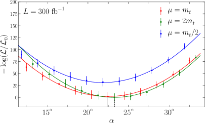
The central scale, $\mu=m_{t}$, is shown in red, while $\mu=2m_{t}$ is depicted in green and $\mu=m_{t}/2$ in blue. The estimator for the CP-mixing angle $\hat{\alpha}$ is determined from the position of the minimum of the Likelihood function for $\mu=m_{t}$, while the statistical uncertainty $\Delta\hat{\alpha}_{\textrm{stat}}$ is deduced from the width of the fitted parabola. The Likelihood functions based on the other two scales allow to estimate the systematic uncertainty $\Delta\hat{\alpha}_{\textrm{sys}}$ by studying the impact of higher-order corrections on the extracted angle. For the assumed $300$ fb^-1 we obtain as estimator for the CP-mixing angle:

$$\hat{\alpha}=22.5^{\circ}\pm 0.9^{\circ}~{}\textrm{[stat.]}~{}^{+0.8^{\circ}}_{-0.6^{\circ}}~{}\textrm{[sys.]}\;,$$ (10)

where the statistical uncertainty is still the dominant error contribution. In Table 1 we also show results for $L=36$ fb^-1 and $L=80$ fb^-1, together with the previously discussed result for $L=300$ fb^-1.

$L~{}[\textrm{fb}^{-1}]$	$\hat{\alpha}$	$\Delta\hat{\alpha}_{\textrm{stat}}$	$\Delta\hat{\alpha}^{+}_{\textrm{sys}}$	$\Delta\hat{\alpha}^{-}_{\textrm{sys}}$
$36$	$23.2^{\circ}$	$\pm 2.4^{\circ}$	$+0.5^{\circ}$	$-0.7^{\circ}$
$80$	$24.2^{\circ}$	$\pm 1.7^{\circ}$	$+0.3^{\circ}$	$-0.9^{\circ}$
$300$	$22.5^{\circ}$	$\pm 0.9^{\circ}$	$+0.8^{\circ}$	$-0.6^{\circ}$

Table 1: The inferred value of the CP-mixing angle and its statistical and systematic uncertainties for several integrated luminosities.

As expected, the statistical uncertainty reduces with increasing luminosity, while the systematic uncertainty is independent of the number of events. We can test this expectation by studying the uncertainty contributions as a function of the luminosity, as illustrated in Fig. 5.

Figure 5: The estimated statistical and systematic uncertainty, $\Delta\hat{\alpha}$ on the extracted CP-mixing angle $\hat{\alpha}$ as a function of the integrated luminosity $L$. The solid lines show a constant and a $1/\sqrt{L}$ fit.

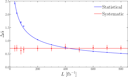
The red square data points represent the systematic uncertainties inferred from the Likelihood analysis while the blue dots correspond to the statistical uncertainty. Note that for this study we used the symmetrised version of the systematic uncertainties. The solid lines depict the fit results assuming a constant for the systematic uncertainties and a $1/\sqrt{L}$ behaviour for the statistical uncertainty. We conclude that the systematic uncertainty inferred from scale variations amounts to a constant $\pm 0.7^{\circ}$ uncertainty. Starting from an integrated luminosity of $L\approx 425$ fb^-1 onwards, the analysis would not improve any more by collecting more data and is limited by the theory uncertainty. However, assuming realistic signal detection efficiencies at the level of a few percent Sirunyan:2018lzm , even for the high luminosity phase of the LHC the NLO predictions would be sufficiently precise. In the long term perspective a determination of the mixing angle could envisaged with an absolute accuracy of $\pm 0.7^{\circ}$.

To conclude, we want to give an estimate for the required integrated luminosity in order to achieve a discovery, i.e. a $5\sigma$ deviation from the SM value $(\alpha=0^{\circ})$, at the LHC for the BSM scenario under consideration. For simplicity we assume that the SM value can be inferred with the same accuracy as the BSM scenario studied before. We find that approximately $20$ fb^-1 are necessary to establish a $5\sigma$ deviation from the Standard Model. Assuming a realistic signal detection efficiency of $3\%$ an integrated luminosity of $300$ fb^-1 allows to establish an excess with $3\sigma$ significance. However, even with this realistic signal detection efficiency a discovery would be possible in the high-luminosity phase of the LHC.

V Conclusions

In this article we study a Standard Model extension which generalizes the top-quark Yukawa coupling to the Higgs boson. In particular, the model allows that the Higgs boson is not a CP eigenstate and interpolates continuously between the SM and a scenario where the relative sign of the top-quark Yukawa coupling with respect to the Higgs boson coupling to $W$ bosons is inverted. We find that for mixing angles up to $25^{\circ}$ a cross section measurement alone cannot distinguish the SM from the BSM scenario.

Simulating a concrete measurement and assuming a signal detection efficiency of $3\%$ we show that using the Matrix Element Method a signal at the $3\sigma$ level can be established with an integrated luminosity of $300$ fb^-1. The high luminosity phase allows a discovery with $5\sigma$ and will not be limited by theoretical uncertainties. As a side effect the paper provides a further illustration of the power of the Matrix Element Method in challenging the Standard Model.

References

- (1) G. Aad et al. [ATLAS Collaboration], “Observation of a new particle in the search for the Standard Model Higgs boson with the ATLAS detector at the LHC,” Phys. Lett. B 716, 1 (2012)
- (2) S. Chatrchyan et al. [CMS Collaboration], “Observation of a New Boson at a Mass of 125 GeV with the CMS Experiment at the LHC,” Phys. Lett. B 716, 30 (2012)
- (3) G. C. Branco, P. M. Ferreira, L. Lavoura, M. N. Rebelo, M. Sher and J. P. Silva, “Theory and phenomenology of two-Higgs-doublet models,” Phys. Rept. 516, 1 (2012)
- (4) K. Agashe, R. Contino and A. Pomarol, “The Minimal composite Higgs model,” Nucl. Phys. B 719, 165 (2005)
- (5) T. Appelquist and M. S. Chanowitz, “Unitarity Bound on the Scale of Fermion Mass Generation,” Phys. Rev. Lett. 59, 2405 (1987) Erratum: [Phys. Rev. Lett. 60, 1589 (1988)].
- (6) A. M. Sirunyan et al. [CMS Collaboration], “Measurement of the top quark Yukawa coupling from kinematic distributions in the lepton+jets final state in proton-proton collisions at 13 TeV,” arXiv:1907.01590 [hep-ex].
- (7) A. M. Sirunyan et al. [CMS Collaboration], “Observation of H production,” Phys. Rev. Lett. 120, no. 23, 231801 (2018)
- (8) M. Aaboud et al. [ATLAS Collaboration], “Observation of Higgs boson production in association with a top quark pair at the LHC with the ATLAS detector,” Phys. Lett. B 784, 173 (2018)
- (9) G. Bordes and B. van Eijk, “On the associate production of a neutral intermediate mass Higgs boson with a single top quark at the LHC and SSC,” Phys. Lett. B 299, 315 (1993).
- (10) F. Maltoni, K. Paul, T. Stelzer and S. Willenbrock, “Associated production of Higgs and single top at hadron colliders,” Phys. Rev. D 64, 094023 (2001)
- (11) M. Farina, C. Grojean, F. Maltoni, E. Salvioni and A. Thamm, “Lifting degeneracies in Higgs couplings using single top production in association with a Higgs boson,” JHEP 1305, 022 (2013)
- (12) S. Biswas, E. Gabrielli and B. Mele, “Single top and Higgs associated production as a probe of the Htt coupling sign at the LHC,” JHEP 1301, 088 (2013)
- (13) P. Agrawal, S. Mitra and A. Shivaji, “Effect of Anomalous Couplings on the Associated Production of a Single Top Quark and a Higgs Boson at the LHC,” JHEP 1312, 077 (2013)
- (14) S. F. Taghavi and M. M. Najafabadi, “Angular Correlations in Associated Production of Single Top and Higgs with and without anomalous Couplings,” Int. J. Theor. Phys. 53, no. 12, 4326 (2014)
- (15) J. Campbell, R. K. Ellis and R. Röntsch, “Single top production in association with a Z boson at the LHC,” Phys. Rev. D 87, 114006 (2013)
- (16) J. Ellis, D. S. Hwang, K. Sakurai and M. Takeuchi, “Disentangling Higgs-Top Couplings in Associated Production,” JHEP 1404, 004 (2014)
- (17) J. Chang, K. Cheung, J. S. Lee and C. T. Lu, “Probing the Top-Yukawa Coupling in Associated Higgs production with a Single Top Quark,” JHEP 1405, 062 (2014)
- (18) A. Kobakhidze, L. Wu and J. Yue, “Anomalous Top-Higgs Couplings and Top Polarisation in Single Top and Higgs Associated Production at the LHC,” JHEP 1410, 100 (2014)
- (19) L. Wu, “Enhancing Production from Top-Higgs FCNC Couplings,” JHEP 1502, 061 (2015)
- (20) C. Englert and E. Re, “Bounding the top Yukawa coupling with Higgs-associated single-top production,” Phys. Rev. D 89, no. 7, 073020 (2014)
- (21) F. Demartin, F. Maltoni, K. Mawatari and M. Zaro, “Higgs production in association with a single top quark at the LHC,” Eur. Phys. J. C 75, no. 6, 267 (2015)
- (22) A. V. Gritsan, R. Röntsch, M. Schulze and M. Xiao, “Constraining anomalous Higgs boson couplings to the heavy flavor fermions using matrix element techniques,” Phys. Rev. D 94, no. 5, 055023 (2016)
- (23) S. D. Rindani, P. Sharma and A. Shivaji, “Unraveling the CP phase of top-Higgs coupling in associated production at the LHC,” Phys. Lett. B 761, 25 (2016)
- (24) V. Barger, K. Hagiwara and Y. J. Zheng, “Probing the Higgs Yukawa coupling to the top quark at the LHC via single top+Higgs production,” Phys. Rev. D 99, no. 3, 031701 (2019)
- (25) C. Degrande, F. Maltoni, K. Mimasu, E. Vryonidou and C. Zhang, “Single-top associated production with a or boson at the LHC: the SMEFT interpretation,” JHEP 1810, 005 (2018)
- (26) V. Khachatryan et al. [CMS Collaboration], “Search for the associated production of a Higgs boson with a single top quark in proton-proton collisions at TeV,” JHEP 1606, 177 (2016)
- (27) A. M. Sirunyan et al. [CMS Collaboration], “Search for associated production of a Higgs boson and a single top quark in proton-proton collisions at TeV,” Phys. Rev. D 99, no. 9, 092005 (2019)
- (28) P. Artoisenet et al., “A framework for Higgs characterisation,” JHEP 1311, 043 (2013)
- (29) M. Cacciari, G. P. Salam and G. Soyez, “FastJet User Manual,” Eur. Phys. J. C 72, 1896 (2012)
- (30) J. Alwall et al., “The automated computation of tree-level and next-to-leading order differential cross sections, and their matching to parton shower simulations,” JHEP 1407, 079 (2014)
- (31) K. Kondo, “Dynamical Likelihood Method for Reconstruction of Events With Missing Momentum. 1: Method and Toy Models,” J. Phys. Soc. Jap. 57, 4126 (1988).
- (32) K. Kondo, “Dynamical likelihood method for reconstruction of events with missing momentum. 2: Mass spectra for 2 2 processes,” J. Phys. Soc. Jap. 60, 836 (1991).
- (33) J. Alwall, A. Freitas, and O. Mattelaer, “The Matrix Element Method and QCD Radiation,” Phys. Rev. D83 (2011) 074010.
- (34) J. M. Campbell, W. T. Giele, and C. Williams, “The Matrix Element Method at Next-to-Leading Order,” JHEP 11 (2012) 043.
- (35) R. Baumeister and S. Weinzierl, “Matrix element method at next-to-leading order for arbitrary jet algorithms,” Phys. Rev. D95 (2017).
- (36) T. Martini and P. Uwer, “Extending the Matrix Element Method beyond the Born approximation: Calculating event weights at next-to-leading order accuracy,” JHEP 1509, 083 (2015)
- (37) T. Martini and P. Uwer, “The Matrix Element Method at next-to-leading order QCD for hadronic collisions: Single top-quark production at the LHC as an example application,” JHEP 1805, 141 (2018)
- (38) T. Martini, “The Matrix Element Method at next-to-leading order QCD using the example of single top-quark production at the LHC,” arXiv:1807.06859 [hep-ph].
- (39) M. Kraus, T. Martini and P. Uwer, “Predicting event weights at next-to-leading order QCD for jet events defined by jet algorithms,” arXiv:1901.08008 [hep-ph].
- (40) G. Cowan, Statistical data analysis. Oxford University Press, 1998.
- (41) B. Abbott et al. [D0 Collaboration], “Measurement of the Top Quark Mass in the Dilepton Channel,” Phys. Rev. D 60, 052001 (1999)
- (42) V. M. Abazov et al. [D0 Collaboration], “A precision measurement of the mass of the top quark,” Nature 429, 638 (2004)
- (43) A. Abulencia et al. [CDF Collaboration], “Precision measurement of the top quark mass from dilepton events at CDF II,” Phys. Rev. D 75, 031105 (2007)
- (44) V. M. Abazov et al. [D0 Collaboration], “Observation of Single Top Quark Production,” Phys. Rev. Lett. 103, 092001 (2009)
- (45) T. Aaltonen et al. [CDF Collaboration], “First Observation of Electroweak Single Top Quark Production,” Phys. Rev. Lett. 103, 092002 (2009)
- (46) G. Aad et al. [ATLAS Collaboration], “Evidence for single top-quark production in the -channel in proton-proton collisions at 8 TeV with the ATLAS detector using the Matrix Element Method,” Phys. Lett. B 756, 228 (2016)