The effect of fluctuating fuzzy axion haloes on stellar dynamics: a stochastic model

Abstract

Fuzzy dark matter of ultra-light axions has gained attention, largely in light of the galactic scale problems associated with cold dark matter. But the large de Broglie wavelength, believed to possibly alleviate these problems, also leads to fluctuations that place constraints on ultra-light axions. We adapt and extend a method, previously devised to describe the effect of gaseous fluctuations on cold dark matter cusps, in order to determine the imprints of ultra-light axion haloes on the motion of classical test particles. We first evaluate the effect of fluctuations in a statistically homogeneous medium of classical particles, then in a similar system of ultra light axions. In the first case, one recovers the classical two body relaxation time (and diffusion coefficients) from white noise density fluctuations. In the second situation, the fluctuations are not born of discreteness noise but from the finite de Broglie wavelength; correlation therefore exists over this scale, while white noise is retained on larger scales, elucidating the correspondence with classical relaxation. The resulting density power spectra and correlation functions are compared with those inferred from numerical simulations, and the relaxation time arising from the associated potential fluctuations is evaluated. We then apply our results to estimate the heating of disks embedded in axion dark haloes. We find that this implies an axion mass $m\ga 2\times 10^{-22}{\rm eV}$. We finally apply our model to the case of the central cluster of Eridanus II, confirming that far stronger constraints on $m$ may in principle be obtained, and discussing the limitations associated with the assumptions leading to these.

1 Introduction

The cold dark matter based scenario has developed into a highly successful model of structure formation (Frenk & White, 2012). The weakly interacting massive particles (WIMPs) at the core of this scenario can be produced with the right abundance, and a cross section of the order expected of standard weak interaction, from an early thermal equilibrium in the radiation era. Yet, extensive direct detection experiments and collider searches have significantly constrained the expected (mass and cross section) parameter space for such particles (Roszkowski et al., 2018; Boveia & Doglioni, 2018; Arcadi et al., 2018). In addition, from the astrophysical viewpoint, WIMP-based virialized structures suffer from several ’small scale’ problems; such as the cusp-core problem, the ’too big to fail’ problem and the overabundance of subhaloes (Del Popolo & Le Delliou, 2017; Bullock & Boylan-Kolchin, 2017, for recent reviews).

There are proposed solutions for such (very possibly related) problems in terms of baryonic physics. For example through dynamical friction mediated coupling with baryonic clumps (El-Zant et al., 2001; El-Zant et al., 2004; Tonini et al., 2006; Romano-Díaz et al., 2008; Goerdt et al., 2010; Cole et al., 2011; Del Popolo et al., 2014; Nipoti & Binney, 2015), or through gas fluctuations arising from star formation or active galactic nuclei (Read & Gilmore, 2005; Mashchenko et al., 2006, 2008; Peirani et al., 2008; Pontzen & Governato, 2012; Governato et al., 2012; Zolotov et al., 2012; Martizzi et al., 2013; Teyssier et al., 2013; Pontzen & Governato, 2014; Madau et al., 2014; Freundlich et al., 2019). Recently, El-Zant et al. (2016) developed a stochastic model for such fluctuations and their effect on the cold dark matter halo cusp, in an attempt to understand the mechanism of central halo ’heating’ and core formation from first principles. In the present study, we find that it has wider applications, particularly concerning potentially observable dynamical effects of the fuzzy dark matter (FDM) composed of ultralight axions.

Ultra light axions, with boson mass $\sim 10^{-22}{\rm eV}$, have long been considered as dark matter candidates in connection to the problems facing CDM (e.g., Peebles, 2000; Goodman, 2000; Hu et al., 2000; Schive et al., 2014b; Marsh & Silk, 2014; Hui et al., 2017; Chavanis, 2018; Nori et al., 2019; Mocz et al., 2019. The earlier history of the subject is reviewed in Chavanis, 2011 and Lee, 2018, the former also considering the case of systems with short range interactions). The long de Broglie wavelength associated with their tiny mass results in ’fuzziness’ in their position that implies finite density Bose-condensate halo cores, instead of cusps, and the dissolution of smaller subhaloes. The field associated with such axions may also play a role in sourcing inflation or late dark energy, and non-thermal production implies that they can come with the right abundance and dynamically behave as WIMPs on larger scales despite their small mass (Marsh, 2016, 2017). In light of the relative waning of the WIMP paradigm, light axion FDM has recently gained ground as viable contenders, namely as an alternative to the baryonic solutions to galactic scale problems from within the CDM scenario. In this context, they are one of several particle physics based proposals, including warm dark matter (e.g., Colín et al., 2000; Bode et al., 2001; Schneider et al., 2012; Macciò et al., 2012; Shao et al., 2013; Lovell et al., 2014; El-Zant et al., 2015) and self-interacting dark matter (e.g., Spergel & Steinhardt, 2000; Burkert, 2000; Kochanek & White, 2000; Miralda-Escudé, 2002; Peter et al., 2013; Zavala et al., 2013; Elbert et al., 2015).

Nevertheless, although the large de Broglie wavelength associated with the ultra-light halo bosons can in principle help solve the core/cusp and potentially associated small scale problems, it is not clear if the scaling of core radii with mass inferred from (dark matter only) simulations can be made to agree with observed scalings (Bar et al., 2019; Deng et al., 2018; Safarzadeh & Spergel, 2019; Robles et al., 2019), and there are additional constraints regarding the particle mass arising from Lyman-$\alpha$ and 21 cm observations (e.g., Kobayashi et al., 2017; Nebrin et al., 2018; Lidz & Hui, 2018) and recently from environment around supermassive black holes (e.g., Davoudiasl & Denton, 2019; Bar et al., 2019; Desjacques & Nusser, 2019; Davies & Mocz, 2019).

A large de Broglie wavelength also leads to reduction of bound substructure, in apparent agreement with observations. But as bound substructure is replaced by broad interference patterns (e.g., Schive et al., 2014a), this is accompanied by density fluctuations that may lead to observable effects on the baryonic components of galaxies and place constraints on the masses of FDM particles (Hui et al., 2017; Bar-Or et al., 2019; Amorisco & Loeb, 2018; Marsh & Niemeyer, 2018 Church et al., 2018). This leads to the following conundrum. For FDM to be effective in solving the small scale problems of CDM, the de Broglie wavelength must be of the order of the scales at which the problems appear (i.e., kpc scale); the masses of the axions must therefore be small enough for their wavelength to reach such scales. But then the associated fluctuations are large, and a delicate balance seems required in order to solve the galactic scale problems of CDM and at the same time not overproduce fluctuations (and avoid unobserved consequences on the baryonic components of galaxies). In other words, sufficiently suppressing such fluctuations may imply axion masses that are too large to solve the small scale problems of the WIMP based structure formation scenario.

The density fluctuations give rise to potential fluctuations, much in the same manner as the gaseous fluctuations studied in El-Zant et al. (2016). Here, we make use of this fact in order to study their effect on the stellar dynamics of galaxies with the aforementioned problem in mind. For this purpose, we adopt and extend the methods outlined there to physically quite distinct, but formally related, contexts: first to derive the standard two body relaxation time, by assuming delta correlated density fluctuations (Section 2); then to estimate the density and force fluctuations in FDM haloes, and to calculate the associated correlation functions and relaxation time of a classical test particle subject to FDM halo fluctuations, pointing out differences and similarities with classical two body relaxation due to discreteness (white) noise (Section 3); and finally, as an application, to estimate the effect of fluctuations of an FDM halo on the Milky Way disk in light of recent observations of the stellar velocity dispersion, putting constraints on the minimal mass of plausible FDM particles (Section 4). In Section 4.3 we compare the resulting constraints to those from other work. In that section, we also discuss the predictions of our present model regarding the expansion of the central star cluster of the dwarf galaxy Eridanus II, as studied in Marsh & Niemeyer (2018) by adopting the original formulation of El-Zant et al. (2016). The technical details associated with that discussion are given in Appendix F. Section 5 summarizes our results and outlines related conclusions.

2 White noise and two body relaxation

We start by considering how the basic theoretical setup introduced in El-Zant et al. (2016) can be directly applied to derive the standard two body relaxation time for the case of a test star moving through an infinite system of randomly distributed ’field stars’ (point particles), of average spatial mass density $\rho_{0}$.

As in the aforementioned work, we Fourier expand the potential $\Phi$ and density contrast $\delta=\frac{\rho({\bf r})}{\rho_{0}}-1$, so that

$$\Phi({\bf r},t)=\frac{V}{(2\pi)^{3}}\int\Phi_{\bf k}(t)e^{i{\bf k.r}}d{\bf k},$$ (1)

and

$$\delta({\bf r},t)=\frac{V}{(2\pi)^{3}}\int\delta_{\bf k}(t)e^{i{\bf k.r}}d{\bf k}.$$ (2)

Here the volume $V$, previously taken to be much larger than the largest fluctuation scales, should be understood to be arbitrarily large when white noise is considered (as we will see below, the largest relevant fluctuation scales are then effectively determined by the argument of a Coulomb logarithm).

We note at the outset that this formulation already incorporates a form of the ’Jean’s swindle’, whereby the potential $\Phi$ is considered to be solely due to fluctuations around the average mass density in an infinite medium that tends to homogeneity on larger scales (e.g., Binney & Tremaine 2008; Bar-Or et al., 2019). However, as opposed to the standard Jeans swindle, it is not used to calculate the self-gravity of the fluctuations but their gravitational effects on a test particle, while neglecting their own self-gravity. It therefore incorporates the analogous ’Chandrasekhar swindle’, implicit in the derivation of the standard two body relaxation time, which evaluates the effect of finite-$N$ fluctuations in an infinite statistically homogeneous medium with no mean field contribution. As all realistic self-gravitating systems are inhomogeneous, application of the ’Jeans-Chandrasekhar’ swindle implicitly involves a local assumption. A systematic study of the steps leading to this approximation in the context of kinetic theory, as well as an exposition of the rich history of treating fluctuations and associated relaxation in gravitating systems, can be found in Chavanis (2013). Here, we just further note that it is in principle possible to incorporate collective effects, due to self gravity, into the kinetic theory of gravitating systems — either while maintaining the assumption of large scale homogeneity (Weinberg, 1993), or for inhomogeneous systems with integrable mean field dynamics, where action angle variables can be used (Heyvaerts, 2010; Chavanis, 2012) — though the resulting formulations require considerable additional mathematical sophistication and are therefore more difficult to extract information from in practice.

In El-Zant et al. (2016) the $\Phi$ and $\delta$ were initially assumed to be time independent. The time dependence was then introduced through the sweeping ansatz used and tested in turbulence theory, whereby small scale fluctuations are ’swept’ — that is passively advected — by large scale velocity fields, which can either represent mean bulk flows (Taylor, 1938), or random large scale flows characterized by a velocity dispersion (Kraichnan, 1964; Tennekes, 1975). The effective assumption in El-Zant et al. (2016) was that all modes are transported by the same sweeping speed. The model is however easy to generalize to the case when each mode travels with its own velocity, drawn from a given distribution (e.g., Wilczek & Narita, 2012; Wilczek et al., 2014). Here we generalize this sweeping hypothesis to the transport of density fluctuations, focusing on classical point particles and FDM systems.

We define a two time density fluctuation power spectrum that is given through the ensemble average

$$\mathcal{P}({\bf k},t,t^{\prime})=V\langle\delta_{\bf k}(t)\delta^{*}_{\bf k}(t^{\prime})\rangle.$$ (3)

For a stationary stochastic process, the time dependence manifests itself solely in terms of $t-t^{\prime}$, for all $t^{\prime}$, reflecting homogeneity in time. We assume that this is the case here, setting $t^{\prime}=0$ without loss of generality. In particular, the equal time power spectrum is

$$\mathcal{P}({\bf k},0)=V\langle|\delta_{\bf k}(0)|^{2}\rangle.$$ (4)

The components $\Phi_{\bf k}(t)$ and $\delta_{\bf k}(t)$ are related via the Poisson equation $\nabla^{2}\Phi=4\pi G\rho_{0}\delta,$ through

$$\Phi_{\bf k}(t)=-4\pi G\rho_{0}\delta_{\bf k}(t)k^{-2},$$ (5)

where $k=|{\bf k}|$. For a configuration that is isotropic on large scales, the force power spectrum is related to the potential fluctuations by

$$\mathcal{P}_{F}({k},t)=V{k}^{2}\langle\Phi_{k}(0)\Phi_{k}(t)\rangle=(4\pi G\rho_{0})^{2}k^{-2}\mathcal{P}({\bf k},t).$$ (6)

For a system that is homogeneous on large scales, the force correlation function, which is the inverse Fourier transform of the force power spectrum, is given by

$$\langle{\bf F}(0,0).{\bf F}(r,t)\rangle =\frac{1}{(2\pi)^{3}}\int\mathcal{P}_{F}({k},t)e^{i{\bf k}.{\bf r}}d{\bf k}$$

$$=\frac{1}{(2\pi)^{3}}\int\mathcal{P}_{F}({k},t)\frac{\sin(kr)}{kr}4\pi k^{2}dk.$$ (7)

2.1 Fixed velocities

We first consider the simplest case, in which all modes move with the same velocity. This connects the sought after derivation of the two body relaxation time to the situation studied in El-Zant et al. (2016), where we assumed a spatial (one time) power law spectrum of the form $\langle|\delta_{k}(0)|^{2}\rangle=Ck^{-n}$, and introduced the time dependence through a constant speed sweeping hypothesis. We proceed in an analogous manner here, but focus on the special case of a white noise density spectrum ($n=0$), appropriate of the expected spectrum of randomly scattered point masses that we take to represent the ’field stars’ through which a test particle moves. As in the case of the standard derivation of the two body relaxation time, the system of field particle point masses is assumed to be spatially homogeneous, beyond the Poisson noise, and the test particle’s unperturbed motion is rectilinear with constant velocity ${\bf v}_{p}$.

In this case, and introducing maximum and minimal cutoff scales, the spatial force correlation function can be written as

$$\langle{\bf F}(0,0).{\bf F}(r,0)\rangle=\frac{D}{r}\int_{k_{m}}^{k_{x}}\frac{\sin(kr)}{k}dk$$

$$=\frac{D}{r}\left[{\rm Si}(k_{x}r)-{\rm Si}(k_{m}r)\right]$$ (8)

where $D=8(G\rho_{0})^{2}\mathcal{P}({\bf k},0)$ and ${\rm Si}$ refers to the sine integral function. For a white noise power spectrum, $\mathcal{P}({\bf k},0)$ is constant. The force correlation function can in principle be inserted into the stochastic equation (e.g., Osterbrock, 1952; El-Zant et al., 2016)

$$\langle(\Delta v_{p})^{2}\rangle=2\int_{0}^{T}(T-t)\langle{\bf F}(0).{\bf F}(t)\rangle dt,$$ (9)

in order to obtain the velocity variance that the test particle acquires as a result of its motion through fluctuating potential of the randomly distributed field particles.

To do this, one has to transform the spatial correlation function into one involving time. In this regard, it is important to note that ${\bf F}(t)$ refers to the force at time $t$ on a test particle, and is thus evaluated along a particle trajectory. As the field is time dependent and the test particle also moves, in fixed (Eulerian) coordinates the relevant force entering into equation(9) is ${\bf F}={\bf F}({\bf r}_{p},t)$, where ${\bf r}_{p}(t)$ refers to the position of the particle at time $t$. This is assumed to be along the unperturbed trajectory (a straight line).

In El-Zant et al. (2016) we incorporated both the time dependence due to the motion of the test particle and the evolution of the fluctuating field by assuming that that latter is ’swept’, moving with its statistical properties ’frozen in’, with constant speed $v_{r}$ relative to the test particle. It is then a simple matter to relate $\langle{\bf F}(0,0).{\bf F}(r,0)\rangle$ and $\langle{\bf F}(0).{\bf F}(r_{p},t)\rangle$. In the current context, an analogous assumption is that the field stars have negligible velocity dispersion and common ’bulk’ velocity ${\bf v}_{f}={\bf v}_{r}+{\bf v}_{p}$, with ${\bf v}_{r}$ being the relative velocity.  In this case, along a particle trajectory, the force correlation function is

$$\langle{\bf F}(0)~{}.~{}{\bf F}(r=v_{r}t)\rangle =\frac{D}{v_{r}t}\int_{k_{m}}^{k_{x}}\frac{\sin(kv_{r}t)}{k}dk$$

$$=\frac{D}{v_{r}t}\left[{\rm Si}(k_{x}v_{r}t)-{\rm Si}(k_{m}v_{r}t)\right].$$ (10)

This may then be inserted into (9), to obtain the velocity dispersion that the test particle acquires as a result of the application of the stochastic force described by the described correlation function:

$$\langle(\Delta v_{p})^{2}\rangle=2D\int\frac{(T-t)}{v_{r}t}\left[{\rm Si}(k_{x}v_{r}t)-{\rm Si}(k_{m}v_{r}t)\right]dt.$$ (11)

As the Sine integral functions in this equation converge to $\pi/2$ when $k_{x}v_{r}t,k_{m}v_{r}t\gg 1$, in this diffusion limit the velocity dispersion increase is dominated by the non-transient term (involving $T$ rather than $-t$ in the bracket multiplying the correlation function in 11). As detailed in Appendix A, one then finds that

$$\langle(\Delta v_{p})^{2}\rangle=\frac{\pi D}{v_{r}}T\ln\frac{k_{x}}{k_{m}},$$ (12)

which has the form of the standard two body relaxation time if the maximal and minimal fluctuation scales are identified with the maximal and minimal impact parameters of classical theory.

For a system of field point particles of mass $m$, randomly distributed with uncorrelated positions and average homogeneous density $\rho_{0}$, the (equal time) spatial density correlation function is

$$\langle\rho(0,0)\rho(\mathbf{r},0)\rangle=\rho_{0}^{2}~{}\langle\delta(0,0)\delta(\mathbf{r},0)\rangle=m\rho_{0}\delta_{D}(\mathbf{r}),$$ (13)

where $\delta_{D}$ refers to the Dirac delta function. The associated power spectrum is simply

$$\mathcal{P}({k},0)=\frac{m}{\rho_{0}}.$$ (14)

This implies that the density fluctuations of the white noise are equally distributed among the modes such that $\langle|\delta|^{2}\rangle=1/N$, with $N=\rho_{0}V/m$ the number of particles within the volume $V$, and $D=8G^{2}m\rho_{0}$. In this case

$$\langle(\Delta v_{p})^{2}\rangle=\frac{8\pi G^{2}\rho_{0}m}{v_{r}}T\ln\Lambda,$$ (15)

where we have set $\Lambda=\frac{k_{x}}{k_{m}}=\frac{\lambda_{\rm max}}{\lambda_{\rm min}}$, $\lambda_{\rm max}$ and $\lambda_{\rm min}$ being the maximal and minimal fluctuation wavelengths. Assuming that the test particle speed $\sim v_{r}\sim v$, then the timescale for the RMS perturbation to the velocity described by (12) to reach a typical speed $v$ is

$$t_{r}=\frac{v^{3}}{8\pi G^{2}\rho_{0}m\ln\Lambda},$$ (16)

which is the standard formula for the two body relaxation time.

2.2 Distribution of field particle velocities

So far we have assumed that all modes are ’swept’ by the same constant velocity field, and by implication (in the case of white noise density fluctuations) that all field particles had the same velocity. It is possible however to extend the sweeping picture to the case when each mode has its own ’advection’ velocity. In the current context this translates into extending the formulation to include a velocity distribution for the field particles. As each mode is passively advected with velocity ${\bf v}$, mass conservation requires that

$$i\frac{\partial\rho_{\bf k}(t)}{\partial t}={\bf k}.{\bf v}~{}\rho_{\bf k}(t),$$ (17)

where $\rho_{\bf k}(t)=\rho_{0}\delta_{\bf k}(t)$. This has for solution

$$\rho_{\bf k}(t)=\rho_{\bf k}(0)e^{-i{\bf k}.{\bf v}t}.$$ (18)

Thus

$$\langle\rho_{\bf k}(0)\rho^{*}_{{\bf k^{\prime}}}(t)\rangle=\rho_{0}^{2}\langle\delta_{\bf k}(0)\delta^{*}_{{\bf k}^{\prime}}(t)\rangle=\rho_{0}^{2}\langle e^{i{\bf k^{\prime}}.{\bf v}t}\delta_{\bf k}(0)\delta^{*}_{{\bf k}^{\prime}}(0)\rangle.$$ (19)

For a homogeneous (in both space and time) stochastic process defined over an infinite spatial volume, equation (2) implies that

$$V^{2}\langle\delta_{\bf k}(0)\delta^{*}_{{\bf k}^{\prime}}(t)\rangle=(2\pi)^{3}\mathcal{P}({\bf k},t)\delta_{D}({\bf k}-{\bf k}^{\prime}),$$ (20)

as the power spectrum is the Fourier transform of the spatial correlation function.

The density correlation function takes a particularly simple form if the density fluctuations are (at least initially) uncorrelated with the velocities; that is, each mode can have any velocity. This will be the case if there is no explicit dispersion relation tying ${\bf v}$ and ${\bf k}$, which is the case of classical particle systems, but not when the fluctuations have quantum origin as discussed later. When no such correlation exists, one can use equations (19) and (20) to derive

$$\mathcal{P}({\bf k},t)=\mathcal{P}({\bf k})\langle e^{-i{\bf k}.{\bf v}~{}t}\rangle;$$ (21)

where, again assuming a homogeneous process, we used $V^{2}\langle\delta_{\bf k}(0)\delta^{*}_{\bf k^{\prime}}(0)\rangle=(2\pi)^{3}\mathcal{P}({\bf k})\delta_{D}({\bf k}-{\bf k}^{\prime})$ and integrated over the delta functions.

Assuming a mass normalized velocity distribution function $f({\bf v})$, such that $\int f({\bf v})d{\bf v}=\rho_{0}$, this leads to

$$\mathcal{P}({\bf k},t)=\frac{\mathcal{P}({\bf k})}{\rho_{0}}\int e^{-i{\bf k}.{\bf v}~{}t}f({\bf{v}})d{\bf v}.$$ (22)

For the case of delta correlated white noise (of equation 13)

$$\mathcal{P}({\bf k},t)=\frac{m}{\rho_{0}^{2}}~{}\int e^{-i{\bf k}.{\bf v}~{}t}f({\bf{v}})d{\bf v}.$$ (23)

Note that this leads to the same wavenumber-frequency power spectrum $\hat{C}({\bf k},\omega)$ as given by equation (23) of Bar-Or et al. (2019). Using equations (6) and (7) one can obtain the force correlation function

$$\langle{\bf F}(0,0).{\bf F}(r,t)\rangle=8~{}G^{2}m\int f({\bf v})d{\bf v}\int\frac{\sin(k|{\bf r}/t-{\bf v}|t)}{k|{\bf r}/t-{\bf v}|t}dk,$$ (24)

which assumes an isotropic medium (but not necessarily isotropic velocities)  Using (9), this gives

$$\begin{split}\langle(\Delta v_{p})^{2}\rangle=&16G^{2}m\int d{\bf v}\frac{f({\bf v})}{|{\bf v}_{p}\!-\!{\bf v}|}\\ &\int_{0}^{T}\!\frac{(T\!-\!t)}{t}\left[{\rm Si}(k_{x}|{\bf v}_{p}\!-\!{\bf v}|t)-{\rm Si}(k_{m}|{\bf v}_{p}\!-\!{\bf v}|t)\right]dt,\end{split}$$ (25)

where we set ${\bf r}={\bf r}_{p}={\bf v_{p}}t$ to represent the time variation due to the test particle’s motion (again, as in standard two body relaxation theory, this is rectilinear), with ${\bf v}$ representing the motion of field particles. Proceeding as previously, while deriving equation (12), we find that in the diffusion limit — which here requires that $k_{m}|{\bf v}_{p}-{\bf v}|t\gg 1$ is reached for all ${\bf v}$ — the test particle’s velocity dispersion increase, as it moves through the fluctuating field, can be expressed as

$$\langle(\Delta v_{p})^{2}\rangle=8\pi mG^{2}T\ln\left(\frac{k_{x}}{k_{m}}\right)\int d{\bf v}\frac{f({\bf v})}{|{\bf v}_{p}-{\bf v}|}.$$ (26)

This reduces to (12) if $f({\bf v})=\rho_{0}\delta_{D}({\bf v}_{f}-{\bf v})$, in which case the relaxation time is given by (16).

Finally, note that the velocity dispersion derived thus, in the diffusion limit, is related to the trace of the diffusion coefficient matrix by $\langle(\Delta v_{p})^{2}\rangle=T\sum_{i=j}D[\Delta v_{i}\Delta v_{j}]$. The individual diffusion coefficients $D_{ij}$ can also be obtained in a similar manner (as detailed in Appendix B).

3 Relaxation induced by fluctuating axion system

The same logic behind the derivations of the classical relaxation time, including the ’sweeping’ assumption used, can be employed to determine the effect of a fluctuating FDM axion field on a classical test particle, with some differences arising from peculiarities connected to the quantum origin of the evolution of the density fluctuations of the axion field.

As FDM axions are by definition ultra light (with masses around $10^{-22}{\rm eV}$), an enormous number of them is needed to constitute a dark matter halo ($\sim 10^{100}$). There is little question here of discreteness noise, the source of classical relaxation discussed above, having much effect; a mean field approximation is therefore warranted. For a system of bosons of mass $m$, interacting only through gravity, this leads to the Schrödinger-Poisson system (Ruffini & Bonazzola, 1969)

$$i\hbar\frac{\partial}{\partial t}\psi({\bf r},t)=-\frac{\hbar^{2}}{2m}\nabla^{2}\psi({\bf r},t)+m~{}\Phi_{s}({\bf r},t)\psi({\bf r},t),$$ (27)

$$\nabla^{2}\Phi_{s}({\bf r},t)=4\pi G~{}|\psi({\bf r},t)|^{2},$$ (28)

where $\Phi_{s}$ is the self consistent gravitational potential.

Since, for the system of bosons so described, there are many particles in the same state, $\psi$ behaves as a classical field. The square of the norm of the wave function is directly proportional to the number of particles around position vector ${\bf r}$ at time $t$, and if $\psi$ is mass normalized (as assumed above) then $|\psi|^{2}$ is the mass density. This is stable when observed, in the sense that the result of observation is not subject to issues such as the collapse of the wave function. The quantum-origin of the dynamics, arising from the large de Broglie wavelength, manifests itself nevertheless through interference patterns and fluctuations ubiquitous in numerical simulations of such systems (e.g., Schive et al., 2014a). The role of $\hbar$ is to set an effective spatial (and mass) scale for the fluctuations, given axion masses $m$ and speeds $v$ (and mean density $\rho_{0}$). It is the effect of those fluctuations on a classical particle that is to be modelled using the methods developed above for discreteness noise.

To mimic the derivation of the two body relaxation time, we again assume an infinite homogeneous medium, while neglecting self gravity of the axion field. In other words we invoke the ’Jeans-Chandrasekhar swindle’ (see discussion in paragraph following equations (1) and (2)). We do this by first setting $\Phi_{s}=0$ in equation (27). To describe the effect of fluctuations, in this context, we replace $\Phi_{s}$ in (28) with $\Phi({\bf r},t)=\Phi_{s}({\bf r},t)-\langle\Phi_{s}({\bf r},t)\rangle$. In this case one can analyze the density and potential fluctuations as in equations (1) and (2), and they will still be related by (5). As this neglects the self-gravity of the fluctuations, they must be much smaller than the Jeans length, which is of the order of the physical size in an actual inhomogeneous system. For the swindle to be valid therefore the de Broglie wavelength must be significantly smaller than the size of the system.

Conservation still requires that the classical density modes $\rho_{\bf k}$ be ’swept’ according to equation (18). This will be the case if

$$\phi_{\bf k}(t)=\phi_{\bf k}(0)e^{-i{\bf k}.{\bf v}t}.$$ (29)

For, if

$$\rho({\bf r},t)=\psi({\bf r},t)\psi^{*}({\bf r},t)=\int\phi_{\bf k}(t)\phi^{*}_{{\bf k}^{{}^{\prime}}}(t)e^{i({\bf k}-{\bf k}^{{}^{\prime}}).{\bf r}}d{\bf k}d{\bf k}^{{}^{\prime}},$$ (30)

and

$$\rho_{\bf k}(t)=\int\psi\psi^{*}e^{i{\bf k}.{\bf r}}d{\bf r}=\int\phi_{{\bf k}^{{}^{\prime}}}(t)\phi^{*}_{{\bf k}^{{}^{\prime}}-{\bf k}}(t)d{\bf k}^{{}^{\prime}}.$$ (31)

Then

$$\rho_{\bf k}(t)=e^{-i{\bf k}.{\bf v}t}\int\phi_{\bf k}^{{}^{\prime}}(0)\phi^{*}_{{\bf k}-{\bf k}^{{}^{\prime}}}(0)d{\bf k}^{{}^{\prime}}=\rho_{\bf k}(0)e^{-i{\bf k}.{\bf v}t}.$$ (32)

On the other hand the free field Schrödinger equation for the axion system,

$$i\hbar\frac{\partial}{\partial t}\psi=-\frac{\hbar^{2}}{2m}\nabla^{2}\psi,$$ (33)

has a solution that can be Fourier expanded as

$$\psi({\bf r},t)=\int\phi_{\bf k}e^{i{\bf k}.{\bf r}-\omega t}d{\bf k}.$$ (34)

This can be rewritten as

$$\psi({\bf r},t)=\int\phi_{\bf k}(t)e^{i{\bf k}.{\bf r}}~{}d{\bf k},$$ (35)

with $\phi_{\bf k}(t)$ given by (29), provided ${\bf k}.{\bf v}=\omega$. That is, if each mode is swept by its phase velocity. As the solution (34) requires that

$$\omega=\frac{\hbar k^{2}}{2m},$$ (36)

the group velocity $\frac{d\omega}{d{\bf k}}=\frac{\hbar{\bf k}}{m}$ of a de Broglie wave packet is double the phase velocity.

In this way the dynamics of the free axion system and its effect on the motion of a classical test particle can be completely described, by invoking the sweeping assumptions of the previous sections and proceeding analogously. Note however an important difference. In the classical point particle case, a mode ${\bf k}$ could be swept by any velocity ${\bf v}$, since ${\bf v}$ was independent of ${\bf k}$. This is not the case here since the velocities are directly dependent on the wave numbers through the nonlinear dispersion relation (36).

3.1 Force correlation function and induced velocity variance

In the context just set, the density contrast power spectrum can be written as

$$\mathcal{P}({\bf k},t)\!=\!\frac{(2\pi)^{3}}{\rho_{0}^{2}}\!\!\int\!\!d{\bf v_{1}}d{\bf v_{2}}f(\!{\bf v}_{1}\!)f(\!{\bf v}_{2}\!)\delta_{D}({\bf k}-m_{\hbar}\!{\bf v}_{d})e\!^{-im_{\hbar}({\bf v}_{c}.{\bf v}_{d})t},$$ (37)

where

$$m_{\hbar}=2m/\hbar,$$ (38)

${\bf v}_{i}=\hbar{\bf k}_{i}/m$ are de Broglie wave packet group velocities, and ${\bf v}_{c}$ and ${\bf v}_{d}$ correspond to the sum and differences of the phase velocities of interfering waves; such that $2{\bf v}_{c}={\bf v}_{1}+{\bf v}_{2}$, and $2{\bf v}_{d}={\bf v}_{1}-{\bf v}_{2}$, as detailed in Appendix C. The above expression assumes that $\langle\phi_{\bf k}\rangle=0$, $\langle\phi_{\bf k}\phi^{*}_{\bf k^{{}^{\prime}}}\rangle=f_{\bf k}({\bf k})\delta_{D}({\bf k}-{\bf k}^{{}^{\prime}})$. The $\phi_{\bf k}$ are thus modes of a complex Gaussian random field. This is consistent with our assumption that the density field is a homogeneous, stationary Gaussian random field, completely characterized by a power spectrum and two point correlation function, with the stochastic dynamics determined by the force two point correlation function (equation 9; see also El-Zant et al., 2016). Physically, this may also be justified if the waves are thought to arrive at the test particle location from large distances and different directions with random phases (cf. Bar-Or et al., 2019), which is consistent with a random mode sweeping hypothesis. Furthermore, we assume that the ${\bf k}$ space distribution function is related to the velocity distribution of the axions by $f_{\bf k}({\bf k}_{i})d{\bf k}_{i}=f({\bf v}_{i})d{\bf v}_{i}$, and the distribution functions are mass normalised such that $\int f({\bf v}_{i})d{\bf v_{i}}=\int f_{\bf k}({\bf k}_{i})d{\bf k}_{i}=\rho_{0}$.

The equal time, spatial power spectra are thus

$$\mathcal{P}({{\bf k}},0) =\frac{(2\pi)^{3}}{\rho_{0}^{2}}\int d{\bf v_{1}}d{\bf v_{2}}f({\bf v}_{1})f({\bf v}_{2})\delta_{D}({\bf k}-m_{\hbar}{\bf v}_{d})$$

$$=\frac{(4\pi)^{3}}{m_{\hbar}^{3}\rho_{0}^{2}}\int d{\bf v}_{c}f({\bf v}_{c}+{\bf k}/m_{\hbar})f({\bf v}_{c}-{\bf k}/m_{\hbar}).$$ (39)

These will be used below, along with the dispersion relation (36), to roughly estimate the random force on a test particle due to fluctuations emanating from an FDM halo.

The force correlation function resulting from Eq. (37) is given by

$$\langle{\bf F}(0,0).{\bf F}(r, t)\rangle=$$

$$\left(\frac{4\pi G}{m_{\hbar}}\right)^{2}\!\!\!\int\!\frac{e^{im_{\hbar}({\bf v}_{d}.{\bf r}-{\bf v}_{c}.{\bf v}_{d}t)}}{v_{d}^{2}}f({\bf v}_{1})f({\bf v}_{2})d{\bf v}_{1}d{\bf v}_{2}.$$ (40)

Because this integral is highly oscillatory for large ${\bf v}_{d}$, one may suppose it is dominated by relatively small values of $v_{d}\ll v_{c}$. If this is the case, $f({\bf v}_{1})$ and $f({\bf v}_{2})$ can be approximated as $f({\bf v}_{c})$. This gives

$$\frac{\langle{\bf F}(0,0).{\bf F}(r,t)\rangle}{(8\pi)^{3}G^{2}m_{\hbar}^{-2}}=\!\int\!\!f^{2}({\bf v_{c}})d{\bf v}_{c}\int\frac{\sin\left(m_{\hbar}v_{d}|{\bf r}/t-{\bf v}_{c}|t\right)}{m_{\hbar}v_{d}|{\bf r}/t-{\bf v}_{c}|t}dv_{d},$$ (41)

since the Jacobian associated to the change of variables equals $8$.

From equation (39), it can be seen that this approximation is effectively equivalent to assuming the long wavelength limit of the spatial power spectrum, which then simply corresponds to white noise. In this context, the integration over ${\bf v}_{d}$ is no longer weighed by convolution with the distribution functions, a situation which can be partly corrected for by appropriate choice of the Coulomb logarithm appearing below. This approach is particularly justified if the distribution function is roughly constant for smaller speeds (larger wavelengths) before sharply cutting off beyond a characteristic value (filtering off smaller wavelengths), as in the case of a Maxwellian. In this case, we explicitly show (end of Section 3.2.1) that the mass fluctuations on large (relative to de Broglie) scales do tend to Poissonian noise, which puts in context the correspondence with the classical two body relaxation that we now derive.

As before, we then use equation (9) and assume a test particle velocity ${\bf v}_{p}$ (recall that the test particle is classical) to obtain

$$\langle(\Delta v_{p})^{2}\rangle= ~{}2(8\pi)^{3}G^{2}m_{\hbar}^{-3}\int d{\bf v}_{c}\frac{f^{2}({\bf v}_{c})}{|{\bf v}_{p}-{\bf v}_{c}|}\int_{0}^{T}\frac{(T-t)}{t}\times$$

$$\left[{\rm Si}\left(m_{\hbar}v_{dx}|{\bf v}_{p}-{\bf v}_{c}|t\right)-{\rm Si}\left(m_{\hbar}v_{dm}|{\bf v}_{p}-{\bf v}_{c}|t\right)\right]dt.$$ (42)

In the diffusion limit this gives,

$$\langle(\Delta v_{p})^{2}\rangle=\left(\frac{4\pi}{m_{\hbar}}\right)^{3}8\pi G^{2}T\ln\Lambda\int d{\bf v}_{c}\frac{f^{2}({\bf v}_{c})}{|{\bf v}_{p}-{\bf v}_{c}|},$$ (43)

where here

$$\Lambda=\frac{v_{dx}}{v_{dm}},$$ (44)

is a ratio of maximal and minimal speeds, related (inversely) to associated wavelengths through the de Broglie relation. We evaluate and further discuss this Coulomb logarithm in specific cases in Appendix E.

If we introduce

$$m_{\rm eff}=\left(\frac{4\pi}{m_{\hbar}}\right)^{3}\frac{\int f^{2}({\bf v})d{\bf v}}{\int f({\bf v})d{\bf v}},$$ (45)

where $m_{\hbar}$ is given by (38) and

$$f_{\rm eff}({\bf v})=\frac{\int f({\bf v})d{\bf v}}{\int f^{2}({\bf v})d{\bf v}}f^{2}({\bf v}),$$ (46)

then equation (43) acquires the same form as (26).

The effective mass and distribution functions found above are as those in Bar-Or et al. (2019), where they enter into expressions for the diffusion coefficients. Our derivation is different in its incorporation and extension of the idea of the sweeping of modes by a ${\bf k}$-dependent velocity field from turbulence theory, in order to obtain the space-time correlation function and power spectrum; and in that it explicitly involves evaluation of the force fluctuations and associated correlation function, with the diffusion limit taken as a final step. In the context of this formulation, it is clear that the effective mass and distribution function are associated with an assumption of white noise spatial power spectrum of density fluctuations, with minimal and maximal cutoffs determined by a Coulomb logarithm. This explains the parallel with softened (but statistically homogeneous on large scales) classical systems, found by Bar-Or et al. (2019). A central difference with classical particle systems, however, is encoded in the quantum-origin correlation of the sweeping velocity and wavenumber of the interfering waves, which sets the particular form of the effective quantities.

Again, as in the case of classical particles, in the diffusion limit, $\langle(\Delta v_{p})^{2}\rangle=T\sum_{i=j}D[\Delta v_{i}\Delta v_{j}]$. Also, the individual diffusion coefficients $D[\Delta v_{i}\Delta v_{j}]$ can be obtained as outlined in Appendix B.

Note however that, as opposed to the situation with equation (26), a delta function distribution in velocities does not lead to an equation analogous to (16), for the growth of velocity dispersion. In particular the effective mass diverges, reflecting the fact that perfect knowledge of the velocity leads to absolute uncertainty in space.

3.2 From density to force fluctuations and relaxation

In this section we compare power spectra and correlation functions of density fluctuations, calculated in the context of the model just presented, to published results from numerical simulations. We also present estimates of the typical force fluctuations connected to the stochastic density field, thus characterized, and rough estimates of the associated relaxation time of a classical test particle moving in the fluctuating force field.

In order to compare with simulations we need to define a density and velocity distribution. The assumption here — as in applications of two body relaxation theory — is that our calculations are locally valid for inhomogeneous systems with local average density $\rho_{0}$.

A realistic FDM halo is expected to follow the Navarro et al. (1996) profile for radii significantly larger than the typical de Broglie wavelength of the FDM; that is beyond the solitonic core (Schive et al., 2014b). In turn, the NFW profile can be well approximated in the intermediate radii $r$ around the maximal rotation speed (of order of the NFW scale length) by an isothermal profile $\rho_{0}\propto 1/r^{2}$ (Chan et al., 2018). Throughout this section we assume such a profile, along with a Maxwellian velocity distribution. Our calculations are therefore strictly valid only at radii larger than that of the solitonic core. We comment briefly on their possible relevance near and inside the core.

3.2.1 Typical Density and mass fluctuations in axion systems

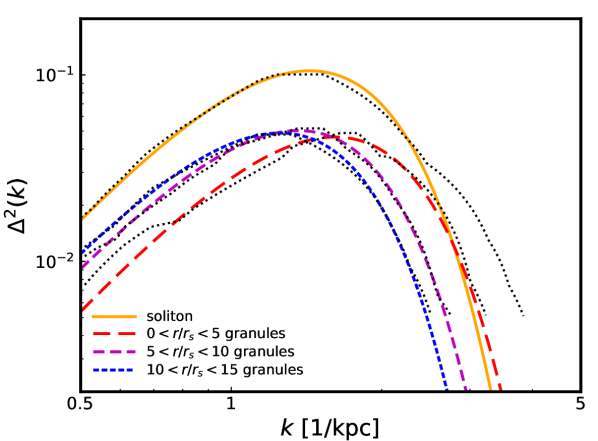
Figure 1: Equal time dimensionless power spectra of density fluctuations. The dotted lines represent (arbitrarily normalized) power spectra inferred from numerical simulation, as presented in Fig 4 (uppermost right hand panel) of Chan et al. (2018). They correspond to power spectra taken within the soliton core $r_{s}$, and in bins $0<r<5r_{s}$, $5r_{s}<r<10r_{s}$ and $10r_{s}<r<15r_{s}$. The solid lines show best (least squares) fits using equations (48) and (49).

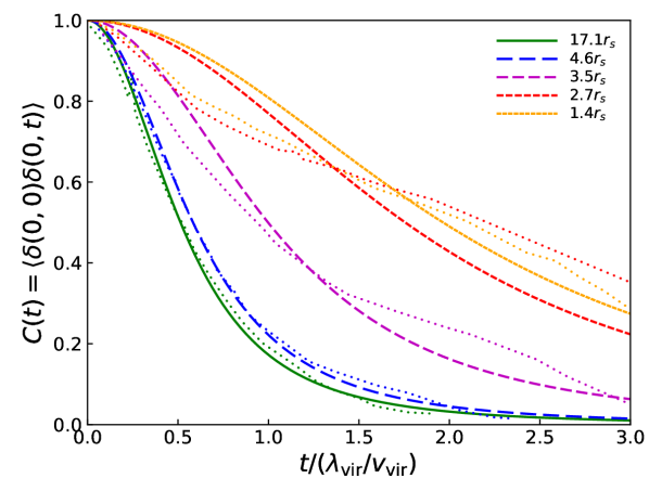
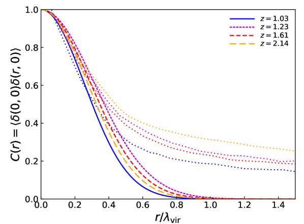
Figure 2: Correlation functions of density fluctuations. The dotted lines show correlation functions inferred from numerical simulations of Veltmaat et al. (2018) (their Fig. 8). The time correlation functions (upper panel) are averaged over denoted multiples of soliton core radii $r_{s}$. The solid lines are best (least squares) fits using equation (50). The lower panel shows the spatial correlation function at different redshifts. In the case of the spatial correlation functions, the fits take into account only points with $r/\lambda_{\rm vir}\leq 0.4$. Here $\lambda_{\rm vir}=\frac{\hbar}{mv_{\rm vir}}$, where $v_{\rm vir}$ is virial velocity. The effective best fit $\lambda$ to the spatial correlation function, obtained by putting $t=0$ in equation (50), range from $\lambda=0.36$ to $\lambda=0.42$ in units of $\lambda_{\rm vir}$. The fits are therefore good up to a scale of order of the effective fitting wavelength.

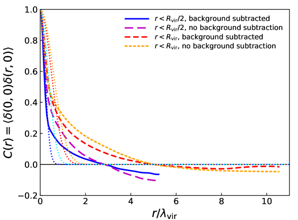
Figure 3: Spatial correlation functions of simulated haloes, evaluated inside the virial radius and half that radius, with and without subtracting the radially averaged halo background density (simulation results kindly made available by Jan Veltmaat). The corresponding best fits using equation (50) are also shown (dotted lines). These are good up to the scales of order of the effective fluctuation scales, and are better inside half the virial radius and when the background density is subtracted. The long correlation tail may reflect the finite spatial size of the fluctuations, non-sphericity of the background halo density, or a radially varying de Broglie wavelength in a realistic halo. The effective wavelengths of the fits (in units of of $\lambda_{\rm vir}=\frac{\hbar}{mv_{\rm vir}}$) are $\lambda_{\sigma}=0.69,0.81$ for correlation functions evaluated inside the virial radius, with and without background subtraction respectively, and $\lambda_{\sigma}=0.3,0.5$ inside half the virial radius, with and without subtraction respectively.

Since, in the case of axion systems, the wave number and velocity distributions are necessarily related, the fluctuation power spectrum is determined by the velocity distribution. If we assume a Maxwellian distribution with one dimensional dispersion $\sigma$,

$$f(v)=\frac{\rho_{0}}{(2\pi\sigma^{2})^{3/2}}e^{-\frac{v^{2}}{2\sigma^{2}}},$$ (47)

the equal time power spectrum given by equation (39) becomes (cf. Appendix D)

$$\mathcal{P}({{\bf k}},0)=\left(\frac{2\sqrt{\pi}}{{m_{\hbar}}\sigma}\right)^{3}e^{-\frac{k^{2}}{\sigma^{2}{m_{\hbar}^{2}}}}.$$ (48)

The dimensionless power spectrum

$$\Delta^{2}(k)=\frac{k^{3}}{2\pi^{2}}\mathcal{P}(k),$$ (49)

measures the contribution to the variance in density fluctuations from logarithmic bins around wave number $k$.

In Fig. 1, we compare what is obtained from this formula with the arbitrarily normalized power spectra from numerical simulations ofChan et al. (2018), who isolated dwarf sized FDM axion haloes from cosmological simulations solving the Schrödinger-Poisson system (27 and 28) self consistently. (The haloes were then evolved along with classical particles representing a stellar distribution. The relevant simulation results for us are those before this latter component is introduced.) As can be seen, the fits are quite good, with some exceptions. Notably at high wavenumbers, inside the solitonic core, where our Maxwellian cutoff at high wavenumber/velocities, appropriate for an isothermal sphere, may not be valid. Outside the core, the peaks move only slightly and the fits thus indeed correspond to a nearly isothermal system. Our a priori assumption of an isothermal system is thus approximately valid outside the core.

Again assuming the Maxwellian distribution of equation (47), and defining an associated wavelength $\lambda_{\sigma}=\hbar/m\sigma=2/m_{\hbar}\sigma$ the correlation function of the density contrast is found (by Fourier transforming 37, cf. Appendix D) to be

$$\langle\delta(0,0)\delta(r,t)\rangle=\frac{1}{(1+\sigma^{2}t^{2}/\lambda_{\sigma}^{2})^{3/2}}e^{-\frac{r^{2}/\lambda_{\sigma}^{2}}{1+\sigma^{2}t^{2}/\lambda_{\sigma}^{2}}}.$$ (50)

Note that $\langle\delta^{2}(0,0)\rangle=1$; the density fluctuations on the smallest scales are therefore of order unity. The variance over all $k$ in density fluctuation contrast, given by

$$\langle\delta^{2}\rangle=\frac{1}{(2\pi)^{3}}\int_{k_{m}}^{k_{x}}\mathcal{P}(k)4\pi k^{2}dk=\int_{k_{m}}^{k_{x}}\Delta^{2}(k)d\ln k,$$ (51)

also tends to unity as $k_{m}\rightarrow 0$ and $k_{x}\rightarrow\infty$.

Fits, using equation (50), to correlation functions presented by Veltmaat et al. (2018) (their figure 8) are shown in Fig. 2. The numerical results of Veltmaat et al. (2018) are based on cosmological simulations using a standard $N$-body code for most of the simulation volume, with high resolution zoom in at selected halo locations solving the Schrödinger-Poisson system. Boundary conditions at the ‘Schrödinger domain’ are imposed via a wave function evolved according to the Hamilton-Jacobi equation.

The fits to the time correlation functions inferred from simulations are good, especially given that they depend on a single parameter. The fits are again better at larger radii. This may be expected, as in addition to our assumption of Maxwellian velocities, the assumption that the fluctuation modes are randomly ’swept’ and come with random phases may not be quite valid at smaller radii. Indeed, as can be seen, at smaller radii the time-correlations display long tails, possibly signaling that the fluctuations are progressively harder to describe by the sweeping of a fluctuating field that corresponds to white noise beyond the de Broglie scale. Though Veltmaat et al. (2018) find persistent oscillations of order $30\%$ even inside the core, these come with a characteristic frequency, with limited spread around it (their figure 7), If not entirely deterministic, the quasi-coherent core oscillations may still have an effect on the stellar dynamics of central bulges and star clusters of the sort described here. This may be further enhanced by coupling to baryonic energy feedback leading to stochastic density and potential fluctuations, (as the oscillations correspond to long lived excitations from the solitonic ground state). But the description of their effect would require modification of the present formulation, in order to take into account the limited frequency spread (we further comment on this in Appendix F).

More puzzling is the behaviour of the spatial correlation function, which displays a quite weak decay tail at large separations. Jans Veltmaat was kind enough to provide correlation functions up to larger scales, with and without radial background density subtracted (shown in Fig. 3). The results are better fit by our model in the former case. Nevertheless, significant discrepancy remains at $r\ga 0.5\lambda_{\rm vir}$, that is at 1 to 1.5 effective wavelengths defined by the best fitting $\lambda_{\sigma}$ (from equation 50 with $t=0$). The correlation tail may be explained if background density correlations remain after the subtraction of the radial averaged density; e.g., because the haloes are not in fact spherical. Indeed, the long tail of the spatial correlation functions tend to mimic those of a purely cold dark matter halo simulated in tandem (Jan Veltmaat, private communication). In addition, the effective size of the the FDM is not small compared to the radial binning, and this ’size’ is not constant but varies with radius, due to changing velocity (and thus de Broglie wavelength) in a realistic halo. The effective size reflected in the $\lambda_{\sigma}$ of our fits thus necessarily reflects an averaging. The fact that our fits are better inside half the virial radius may point to effects of changing velocity dispersions not taken into account by our isothermal model.

The long correlation tail may appear to contradict the much better fits we obtained to the fluctuation power spectra of Chan et al. These, as we saw above, are consistent with our model. At larger scales they generally correspond to a white noise power spectrum (flat $\mathcal{P}(k)$ with $\Delta^{2}\sim k^{3}$). This agreement could be because the power spectra do not go to large enough scales for discrepancies due to the background density correlations to appear. Also, except for the red line in Fig 1, which indeed shows some excess power on larger scales, the Chan et al. spectra are evaluated over radial shells rather than inside spherical bins, which leaves less room for effects due to background density and velocity profiles (although the same general form of the power spectra also arises for the self consistent equilibrium haloes built by Lin et al., 2018, where spherical bins were used; their figure 7c).

If not an artifact arising from the definition and subtraction of the background density, the spatial correlation function of Veltmaat et al. would imply large scale correlations that cannot be captured by the calculated correlation functions — at least while keeping to isothermal Maxwellian systems — as the model predicts mass fluctuations that decay as Poisson noise beyond the de Broglie wavelength, consistent with the white noise power spectrum at larger scales. This can be explicitly shown by calculating the variance a filtering scale $R$, which is given by (e.g., Martínez & Saar, 2002; Mo et al., 2010)

$$\sigma_{R}^{2}=\frac{1}{2\pi^{2}}\int_{0}^{\infty}W^{2}(k,R)\mathcal{P}(k)k^{2}dk,$$ (52)

where $W$ is the Fourier transform of the window filtering function. Using a Gaussian filter, such that $W^{2}(k,R)=e^{-R^{2}k^{2}/2}$ gives,

$$\sigma_{R}^{2}=\left(\frac{2}{(R\sigma m_{\hbar})^{2}+2}\right)^{3/2},$$ (53)

which shows the mass variance to be of order one on scales smaller than the typical de Broglie wavelength of FDM particles and decreasing as $1/R^{3}$ on larger scales, as expected of Poisson noise.

3.2.2 Force fluctuations and rough estimates of the relaxation time

The mean square of the force fluctuations can be obtained from equation (41)

$$\langle F^{2}(0,0)\rangle=(8\pi)^{3}G^{2}m_{\hbar}^{-2}v_{dx}\int f^{2}({\bf v})d{\bf v},$$ (54)

where we have assumed that $v_{dx}\gg v_{dm}$. Recalling that $\int f({\rm v})d{\bf v}=\rho_{0}$, Eq.  (45) yields

$$\langle F^{2}(0,0)\rangle=8~{}G^{2}\rho_{0}m_{\hbar}v_{dx}m_{\rm eff}.$$ (55)

If $v_{dx}\approx\frac{\hbar k_{{x}}}{2m}$, and the maximum wave number is related to the minimal wavelength by $k_{{x}}=2\pi/\lambda_{{x}}$, then

$$\langle F^{2}(0,0)\rangle=16~{}\pi G^{2}\rho_{0}\frac{m_{\rm eff}}{\lambda_{x}}.$$ (56)

A quite crude, but instructive, estimate of the growth of the mean squared speed and associated relaxation time can then be obtained from assuming that the diffusion process determining the growth can be described by a collection of independent ’kicks’, each of duration $\Delta t$, such that after $n$ kicks

$$\langle(\Delta v_{p})^{2}\rangle\approx n\langle F^{2}(0,0)\rangle(\Delta t)^{2}.$$ (57)

Or, using equation (56),

$$\langle(\Delta v_{p})^{2}\rangle\approx\frac{8\pi G^{2}\rho_{0}m_{\rm eff}}{v_{r}}T.$$ (58)

Here $T=n\Delta t$ and we assumed a typical test particle velocity relative to the axions system modes $v_{r}$ and that $\Delta t$ is equal to a half-mode modulation time of the minimal wavelength, such that $\Delta t=\frac{\lambda_{\rm min}}{2v_{r}}$. Although equation (58) is the same as (12) — if $\ln\Lambda=1$ and $m$ replaced by the effective mass — as noted above, a velocity distribution of FDM axion velocities must be defined if this $m_{\rm eff}$, and consequently $\langle(\Delta v_{p})^{2}\rangle$, does not diverge. For the Maxwellian distribution (47)

$$m_{\rm eff}=\frac{8\pi^{3/2}\rho_{0}}{m_{\hbar}^{3}\sigma^{3}}.$$ (59)

A better estimate of the increase in velocity dispersion due FDM density and force fluctuations can be obtained by calculating the diffusion coefficients calculated in Appendix B. In this way

$$\langle(\Delta v_{p})^{2}\rangle=T\sum_{i=j}D[\Delta v_{i}\Delta v_{j}]=T\left(D[(\Delta v_{\parallel})^{2}]+D[(\Delta v_{\perp})^{2}]\right).$$ (60)

For a Maxwellian velocity distribution this gives

$$\langle(\Delta v_{p})^{2}\rangle=T\frac{\sqrt{2}~{}4\pi G^{2}\rho_{0}m_{\rm eff}\ln\Lambda}{\sigma_{\rm eff}}\left[\frac{{\rm erf}(X_{\rm eff})}{X_{\rm eff}}\right].$$ (61)

Here $\sigma_{\rm eff}=\sigma/\sqrt{2}$ and $m_{\rm eff}$ is given by (59) and $X_{\rm eff}=v_{p}/(\sqrt{2}\sigma_{\rm eff})=v_{p}/\sigma$. Thus we have

$$\langle(\Delta v_{p})^{2}\rangle=T\frac{8\pi G^{2}\rho_{0}m_{\rm eff}\ln\Lambda}{v_{p}}{\rm erf}(X_{\rm eff}).$$ (62)

If $v_{p}\sim v_{r}$ and is set to $\sqrt{3}\sigma$ then ${\rm erf}(X_{\rm eff})=0.99$, and with replacement of $m$ with the appropriate $m_{\rm eff}$, this expression is again virtually equivalent to (12). The time for the fluctuations to induce a velocity dispersion of the order of $v_{p}$ is accordingly also given by (16), with $m_{\rm eff}$ in the denominator.

4 The heating of disks by FDM axions

4.1 First estimate

If one wishes to obtain a rough estimate of the role of the fluctuating force in FDM haloes in significantly increasing the velocity dispersion of embedded disk stars, then $v_{p}$ in equation (62) can be replaced by the circular velocity $v_{\rm circ}$ and again ${\rm erf}(X_{\rm eff})\approx 1$. Without taking into account the disk’s self gravity, the relaxation timescale, taken to produce a velocity variance in the motion of the disk stars $\sigma_{d}^{2}$ ($\sigma_{d}$ being the dispersion), is

$$t_{r}\approx\frac{\sigma_{d}^{2}v_{\rm circ}}{8\pi G^{2}\rho_{0}m_{\rm eff}\ln\Lambda},$$ (63)

where $\sigma_{d}^{2}=\sigma_{z}^{2}+\sigma_{R}^{2}+\sigma_{\theta}^{2}$, when measured in cylindrical coordinates moving at the local circular velocity. To estimate this timescale, we assume the FDM halo outside the core to be represented by an isothermal distribution with radial mass density

$$\rho_{0}=\frac{\sigma^{2}}{2\pi Gr^{2}},$$ (64)

with associated circular speed $v_{\rm circ}=\sqrt{2}\sigma$. For this density distribution

$$m_{\rm eff}=\frac{4\sqrt{2\pi}}{Gm_{\hbar}^{3}v_{\rm circ}r^{2}}.$$ (65)

Using equations (63), (64) and (65) we thus find for for the Milky Way solar neighbourhood

$$t_{r}=\frac{1.1\times 10^{12}}{\ln\Lambda}\left(\frac{r}{8~{}{\rm kpc}}\right)^{4}\left(\frac{m}{10^{-22}{\rm eV}}\right)^{3}\left(\frac{\sigma_{d}}{70~{}{\rm kms^{-1}}}\right)^{2}{\rm yr}.$$ (66)

In Appendix E we estimate the Coulomb logarithm argument as

$$\Lambda=36.9\left(\frac{r}{8{\rm kpc}}\frac{m}{10^{-22}{\rm eV}}\frac{v_{\rm circ}}{200{\rm km/s}}\right)^{1/2},$$ (67)

so that $\ln\Lambda=3.6$.

Thus for solar neighbourhood parameters this simple estimate suggests that the mass of the FDM axion should not be less than $\sim 0.36\times 10^{-22}{\rm eV}$ if the local velocity dispersion resulting from fluctuation arising from FDM heating through a Hubble time is not to exceed that observed.

It is remarkable that the estimate of the relaxation time in equation (66) does not depend on the disk circular velocity. On the other hand, observations suggest a clear correlation between velocity dispersion in disks and their maximal rotation speeds (Bottema, 1993; Kregel & van der Kruit, 2005; Kregel et al., 2005). We also note that equation (66) implies a velocity dispersion increase that scales in time diffusely as $\sim t^{1/2}$. As we will see below this applies to both vertical and radial velocity dispersion. However the latter is observed to scale as $\sim t^{1/3}$. Such discrepancies imply that only a small fraction of the velocity dispersion in disks can result from FDM axion fluctuations as treated here. Otherwise, the aforementioned scalings will not be reproduced.

4.2 Vertical and radial dispersion and disk response

The estimate just presented, of the increase in disk star velocity dispersion, did not distinguish between vertical and radial increase. It also did not take into account, even in an approximate manner, the disk self gravity. To make progress on such issues we make use of the formulation of Binney & Tremaine (2008, Section 7.4), exploiting the fact that the effect of fluctuations in FDM axion haloes is expected to be effectively equivalent to that of quasi-particles of mass $m_{\rm eff}$ and distribution function $f_{\rm eff}$.

In this context, the rate of energy transfer, per unit mass, to disk stars in the vertical direction is

$$D[\Delta E_{z}]=D\left[\Delta\left(\frac{1}{2}v_{z}^{2}\right)\right]=v_{z}D[\Delta v_{z}]+\frac{1}{2}D[(\Delta v_{z})^{2}].$$ (68)

Assuming again a Maxwellian FDM velocity distribution and stellar motion with circular velocity $v_{\rm circ}$, writing the diffusion coefficients in terms of components parallel and normal to the motion (Appendix B), and ignoring terms suppressed by factors $(v_{z}/v_{\rm circ})^{2}$, one finds

$$D[\Delta E_{z}] =\frac{1}{4}D[(\Delta v_{\perp})^{2}]$$

$$=\frac{\sqrt{2}\pi G^{2}\rho_{0}m_{\rm eff}\ln\Lambda}{\sigma_{\rm eff}}\left[\frac{{\rm erf}(X_{\rm eff})-{\rm G_{\rm eff}}(X_{\rm eff})}{X_{\rm eff}}\right],$$ (69)

where $m_{\rm eff}$ and $f_{\rm eff}(v)$ are given by (45) and (46) and $X_{\rm eff}=v_{p}/(\sqrt{2}\sigma_{\rm eff})\approx v_{\rm circ}/\sigma$, for nearly circular orbits. Then, using equation (64) and $v_{\rm circ}=\sqrt{2}\sigma$,

$$D[\Delta E_{z}]=0.39\frac{Gm_{\rm eff}v_{\rm circ}}{r^{2}}\ln\Lambda.$$ (70)

If one assumes the virial relation for a system of self gravitating sheets to approximate a disk system $E_{z}$ is related to the vertical velocity dispersion $E_{z}=\frac{3}{2}\sigma_{z}^{2}$ (alternatively, the epicyclic approximation leads to $E_{z}=\sigma_{z}^{2}$; Lacey & Ostriker (1985)). Thus $d\sigma_{z}^{2}/dt=\frac{2}{3}D[\Delta E_{z}]$. Integrating this, and using (70) and (65) one finds

$$\sigma_{z}=2.4~{}{\rm km/s}\\ \left(\frac{10^{-22}{\rm eV}}{m}\right)^{3/2}\left(\frac{8{\rm kpc}}{r}\right)^{2}\left(\frac{T}{10{\rm Gyr}}\right)^{1/2}\ln\Lambda^{1/2}$$ (71)

Note again that the results do not depend on the circular speed associated with the isothermal halo.

As in the previous subsection, if we consider the vertical dispersion of stars to arise solely from the FDM axion fluctuations then the above leads to the relatively weak constraint of $m\ga 0.3\times 10^{-22}{\rm eV}$, if the maximal vertical velocity dispersion in the solar neighborhood taken to be about $30{\rm km/s}$.

This constraint can be tightened by considering the radial dispersion. A similar analysis to that outlined above (again. following the calculation of the aforementioned section of Binney & Tremaine) shows that $\sigma_{R}=1/0.53\times\sigma_{z}$. Therefore

$$\sigma_{R}=4.5~{}{\rm km/s}\left(\frac{10^{-22}{\rm eV}}{m}\right)^{3/2}\!\left(\frac{8{\rm kpc}}{r}\right)^{2}\!\left(\frac{T}{10{\rm Gyr}}\right)^{1/2}\!\!\ln\Lambda^{1/2}$$ (72)

This is inconsistent with observations, as it predicts $\sigma_{R}\sim\sigma_{z}\sim t^{1/2}$, while a power law more akin to $\sigma_{R}\sim t^{1/3}$ is suggested by the observations, a result exhaustively confirmed by the recent data of Mackereth et al. (2019).

The origin of the observed age velocity dispersion relation in discs is not entirely understood. Contributions traditionally considered in the literature include secular processes arising from scattering of stellar trajectories by molecular clouds and spiral arms (cf. Section 5,2 of Mackereth et al., 2019 for a discussion of their possible relative contribution in light of their data). The correlation could, on the other hand, reflect the formation history of a once gas rich disk, rather than secular evolution (e.g. Bournaud et al., 2009; Vincenzo et al., 2019). If we assume that, due to the lack of proper correlation in $\sigma_{R}(t)$, FDM fluctuations are marginal in deciding the disc velocity dispersions, and that therefore only the errors in their $\sigma_{R}$ can be tolerated as being due to FDM fluctuations, this is equivalent to setting $\sigma_{R}\sim 3{\rm km/s}$ in (72), which corresponds to $m\ga 2\times 10^{-22}{\rm eV}$.

4.3 Comparison with other work

Hui et al. (2017) estimate the effect of FDM fluctuations on disk thickness by assuming that they can be modelled as due to classical particles with effective mass corresponding to that enclosed within half a de Broglie wavelength $\lambda_{\rm DB}$. Their equation (35) implies that the effect is entirely dominated by encounters with minimal impact parameters $b_{\rm min}$, without the usual two dimensional integration over impact parameters that leads to the Coulomb logarithm. The notion that adiabatic fluctuations do not contribute to stochastic increase in velocity dispersion envisioned in standard relaxation theory (cf. Appendix E and Church et al., 2018), is taken into account by dividing this minimal $b_{\rm min}$ by the disk half-thickness. Their equation (37), although strictly valid for axion masses $>10^{-22}{\rm eV}$, gives constraints on the FDM mass from disk velocity dispersion in the solar neighbourhood that are only slightly weaker than those we find here, where we have evaluated the combined dynamical effect of the full spectrum of contributing Fourier modes (which leads to the Coulomb logarithm evaluated in Appendix E). Application of their equation (36) on the other hand, relaxes the constraints on the mass much more significantly.

The effect of FDM fluctuations on the vertical dispersion of galactic disks were also discussed by Church et al. (2018). When we assume, as they do, that all the vertical disk dispersion is due to FDM halo fluctuations, we get a similar but weaker constraint of $\sim 0.3\times 10^{-22}{\rm eV}$ on the FDM particle mass (instead of their $0.6$). There are several possible reasons that can account for this difference. As that work was largely concerned with heating due to classical subhaloes, the FDM fluctuations are derived by assuming classical particles of effective mass $M_{\omega}$ (their Eq. 18), and directly applying standard two body relaxation theory. The diffusive effects are also not resolved into vertical and parallel components (associated with the vertical and parallel diffusion coefficients derived here). Furthermore, the effective mass of the FDM quasiparticles is $6.7$ times our $m_{\rm eff}$ (note that there seems to be a typo in their Eq. 24a, with a factor of $\sqrt{2}/4$ apparently missing). Under their assumptions, the Coulomb logarithm is also expected to be larger than evaluated here (Appendix E). Finally, their formulation of the disk response (their equation 25) is different in two ways than assumed here: the factor $\kappa$ in the second term is in our case $1/3$ instead of 0.52 (cf. discussion following Eq. 70 above), and their formulation includes an extra term describing the effect of mass accretion, which we ignore. This term is always positive, and thus increases further the effect of FDM fluctuations, but the other difference mentioned above can account for the discrepancy of a factor of about two in FDM mass constraint.

When, by noting that the increase in disk dispersion due to FDM fluctuations violates the scaling relations between $\sigma_{R}$ and $v_{\rm circ}$, and its time dependence (predicted as $\sigma_{R}\sim t^{1/2}$, instead of the observed $\sim t^{1/3}$), we can derive tighter constraints on the mass of the FDM axion. Namely $m\ga 2\times 10^{-22}{\rm eV}$. This is similar to that derived by Amorisco & Loeb (2018) from the effect of fluctuations on the dynamics of stellar streams in the Milky Way. It is significantly weaker however than that found by Marsh & Niemeyer (2018) by applying the fluctuation model of El-Zant et al. (2016) to the central star cluster ultrafaint Dwarf Galaxy Eridanus II.

As shown in Appendix F, directly applying our extended and improved model to the dynamics central cluster of Eridanus II leads to the similarly strong constraint $m\geq 8.8\times 10^{-20}{\rm eV}$, given one assumes that the FDM makes up all the dark matter and the effect associated fluctuations goes entirely into expanding the cluster, in the manner envisaged by Marsh & Niemeyer (2018). However, for masses $m\ga 10^{-20}{\rm eV}$ the cluster should lie inside the solitonic core of the FDM distribution (Marsh & Niemeyer, 2018). Strictly speaking, one can thus not rule out masses below this using the methods presented here; the eliminated FDM mass range is thus limited (to $10^{-20}{\rm eV}\la m\la 10^{-19}{\rm eV}$), and does not include the range most interesting for solving galactic scale problems of CDM.

To extend the constraint on $m$ to lower values, Marsh & Niemeyer (2018) consider diffusion due to FDM central soliton core oscilations. It may also be the case that fluctuations from FDM granules outside the core could still affect the evolution of a cluster stars inside it. However, as discussed in the aforementioned appendix, even leaving aside doubts about the possibility of direct applicability of our formulation (or that in El-Zant et al., 2016) in drawing quantitative conclusions in such situations, another problem arises. For $m=10^{-20}{\rm eV}$, the minimum wavelength $\lambda_{\rm min}$ of the fluctuations is actually more than an order of magnitude larger than the assumed initial cluster size. And as $\lambda_{\rm min}\sim 1/m$, for smaller masses $\lambda_{\rm min}$ is larger still. It is therefore unclear whether the fluctuations (including coherent core oscillations) would affect the internal structure of the cluster rather than the cluster as a whole.

This places another limitation on obtaining strict constraints from the observed size of the central cluster of Eridanus II. At the same time, however, when the effective FDM granule mass is larger than that of the cluster, one may expect energy equipartition between FDM quasiparticles and the cluster to result in significant motion of its centre of mass. As briefly discussed in the appendix, the displacement of the cluster form the centre of the galaxy, rather than its size, could in this case lead to constraint on $m$. However, a detailed examination of this issue is beyond the scope of the present study.

5 Conclusion

In this study, we first extended the model of El-Zant et al. (2016) to systems of classical point particles with spatial distributions that are statistically homogeneous, up to finite $N$ fluctuations. The associated power spectrum of density fluctuations is flat, corresponding to white noise. This case was not considered in El-Zant et al. (2016), where we developed a model linking (random Gaussian) density fluctuations in a gaseous medium to potential fluctuations that can transform dark halo cusps into cores. In this case, the relevant dependence of the power spectrum on wave number is primarily of the form of a power law ($\mathcal{P}(k)\sim k^{-n}$, with $n<0$).

Application to white noise power spectrum leads to the standard two body relaxation time (if the maximal and minimal impact parameters are associated with maximal and minimal cutoffs in the flat power spectrum of density fluctuations; Section 2.1). This is not all that surprising, as we evaluate the dynamical effects of finite-$N$ fluctuations on the motion of a test particle, while ignoring their self gravity and the mean field (what we termed the ’Jeans-Chandrasekhar Swindle’). These are the assumptions from which the usual two body relaxation time is derived, albeit by different means.

In El-Zant et al. (2016) we used the sweeping hypothesis, widely employed in turbulence theory, to transform spatial power spectra into the time domain, while assuming that all density fluctuation modes moved with the same velocity. Here we extend this by allowing each Fourier mode to be ’swept’ with its own velocity and imposing mass conservation to determine its time evolution (Section 2.2). If the mode velocities are uncorrelated with wavenumber (as expected of a homogeneous classical system), there arises a particularly simple relationship linking the spatio-temporal power spectrum to the spatial (equal time) power spectrum and the velocity distribution function (equation 21). This then naturally leads to the full set of diffusion coefficients associated with standard relaxation theory (Appendix B).

Next we consider systems of ultralight FDM axions, in the mean field limit and again assuming spatial homogeneity on large scales. Given the aforementioned limit, the fluctuations here are not due to finite $N$ effects, but rather to the large de Broglie wavelength associated with the ultralight particles. The Jeans-Chandrasekhar swindle here requires that the de Broglie wavelength is small enough so that the self gravity of the fluctuations can be ignored — that is much smaller than the Jeans length, which is of the order of the size of the physical system to be modelled. The sweeping hypothesis, generalized as described above, can still be used to obtain the spatio-temporal density power spectrum, and from this the force power spectrum and correlation function. As in the case of gaseous fluctuations and classical point particle systems, the force correlation function can be inserted into a stochastic equation to evaluate the effect of relaxation due to the fluctuations and the associated timescale.

There are two main differences with the classical case nevertheless. Although the relevant Schrödinger equation is that of a classical field (given the large number of bosons assumed to share the same states), the wave nature of the field naturally links the velocities at which Fourier density fluctuation modes can move to their wavenumber; velocities and wavenumbers are therefore no longer uncorrelated, and mass conservation now requires that the wave function modes be swept at a frequency-wavenumber dependent phase velocity. Furthermore, the usual quantum interference between wave function modes is present. The interference pattern, arising from associating the density with the square of the wave function, leads to a power spectrum that is dependent on products of pairs of wavenumber (or equivalently velocity) distribution functions.

In the diffusion limit, the effect of the FDM fluctuations on the motion on a classical test particle (namely in terms of increase in velocity dispersion), can still be written in the form familiar from standard two body relaxation theory. However the said interference effects imply that the resulting quasi-particles, through which the association with classical relaxation theory is made, have effective mass and distribution function that involves integrals of the square of the velocity distribution function of the FDM axions. The resulting diffusion coefficients are equivalent to those derived in Bar-Or et al. (2019), though our approach involves explicit evaluation of the force correlation function, with the diffusion limit taken as a final step.

In the context of the present formulation, it becomes apparent that the procedure leading to the aforementioned effective quantities (and description in terms of quasiparticles), practically entails taking the long wavelength limit. This is in turn associated with a white noise spatial power spectrum of density fluctuations on scales larger than the de Broglie wavelength. In light of this approximation, a Coulomb logarithm arises; its choice determines the range of modes contributing to the white noise spectrum. This approach is particularly well motivated when the distribution function is nearly constant for smaller velocities (larger wavelengths), before sharply cutting off beyond a characteristic value (Section 3.1; Appendix E).

This is the case, for example, for a Maxwellian velocity distribution. We derive explicit expressions for the power spectrum and correlation function of FDM density fluctuations and the mass fluctuations on different scales in this case (Section 3.2.1). These are of order one on scales of the order of the de Broglie wavelength and smaller, and then decay as Poisson noise on larger scales. As expected, the associated spectrum is flat (corresponding to white noise) on scales that are significantly larger than the de Broglie wavelength of the FDM axions, with a cutoff on smaller scales. This trend fits quite well the power spectrum from the numerical simulations of Chan et al. (2018). We also compare our results with correlation functions computed from numerical simulations by Veltmaat et al. (2018). Our time correlation functions nicely match theirs (especially when those are averaged over larger spherical regions). Their spatial correlation functions are well fit on smaller scales. They then however display a weakly declining tail at large scales that is not captured by our Gaussian decay. This could be possibly related to residual correlations of the background density that remain after subtracting the radially averaged density field; for example, due to the non-sphericity of the halo and the finite size of the fluctuations, which also varies with radius due to changing de Broglie wavelength.

We also estimate the effect of FDM fluctuations on galactic disks. If the total vertical velocity dispersion in the solar neighbourhood is attributed to such fluctuations, the FDM axion is constrained to have a mass $m\ga 0.3\times 10^{-22}{\rm eV}$. Noting however the $\sim t^{1/3}$ growth of radial velocity dispersion with time implied by observations, further constraint can be inferred. This is because the growth described by our diffusive model is necessarily $\sim t^{1/2}$, which contradicts the extensive recent study of Mackereth et al. (2019). Reasoning that the FDM fluctuation contribution to the radial dispersion should therefore be limited to the errors in the aforementioned data, in order to avoid inconsistency, we find $m\ga 2\times 10^{-22}{\rm eV}$ (Section 4.2).

This latter constraint is similar those obtained by Amorisco & Loeb (2018) from evaluation of the effect of fluctuations on the dynamics of stellar streams, and also those inferred from the dynamics of dark matter dominated objects such as dwarf and ’ultra-diffuse’ galaxies (e.g., Wasserman et al., 2019). It is however significantly weaker than those obtained by directly applying the model of El-Zant et al. (2016) to the central star cluster of the ultrafaint dwarf galaxy Eridanus II (Marsh & Niemeyer, 2018). We applied our extended and generalized model to that situation, confirming that similar constraints can in principle be derived under the same assumptions, while discussing the limitations associated with these assumptions (Section 4.3 and Appendix F).

The constraints from the disk dynamics derived here are also weaker than those inferred through entirely different means, such as Lyman-$\alpha$ (Kobayashi et al., 2017; Nori et al., 2019) and 21 cm observations (Nebrin et al., 2018; Lidz & Hui, 2018), and the environment around supermassive black holes (e.g., Davoudiasl & Denton, 2019; Bar et al., 2019; Desjacques & Nusser, 2019; Davies & Mocz, 2019). While these methods are subject to their own uncertainties, our model for the effect of FDM fluctuations on disks, on the other hand, only takes into account the disk self gravity in the simplest possible way (by applying the vertical virial theorem; Section 4.2). The disk self-gravitating response may in principle modify the effect of fluctuations. If it is similar in nature to the response of the nonradial modes in the perturbed haloes studied in El-Zant et al. (2016), it may in fact significantly amplify and enhance the effect of the imposed stochastic fluctuations. This should be worth studying in detail in future work, as in a disk such effects may in fact be expected to be even more prominent.

Appendix A Velocity dispersion for a white noise power spectrum

Adapting the theoretical framework introduced in El-Zant et al. (2016) to a test particle affected by stationary stochastic density fluctuations with a time-dependent white noise power spectrum, resulting from all modes move with the same velocity $v_{r}$ relative to the test particle, yields a velocity dispersion after time $T$ given by Eq. (11). This equation is the sum of

$$\langle(\Delta v_{p})^{2}\rangle_{1}=\frac{2DT}{v_{r}}\int_{0}^{T}\frac{{\rm Si}(k_{x}v_{r}t)-{\rm Si}(k_{m}v_{r}t)}{t}dt$$ (73)

and

$$\langle(\Delta v_{p})^{2}\rangle_{2}=-\frac{2D}{v_{r}}\int_{0}^{T}\left[{\rm Si}(k_{x}v_{r}t)-{\rm Si}(k_{m}v_{r}t)\right]dt,$$ (74)

where $2\pi/k_{m}$ and $2\pi/k_{x}$ are the maximum and minimum cutoff scales of the power spectrum and Si denotes the Sine integral function. These two terms can be rewritten as

$$\langle(\Delta v_{p})^{2}\rangle_{1}=\frac{2DT}{v_{r}}\left[\int_{0}^{u_{x}}\frac{{\rm Si}(u)}{u}du-\int_{0}^{u_{m}}\frac{{\rm Si}(u)}{u}du\right]$$ (75)

and

$$\langle(\Delta v_{p})^{2}\rangle_{2}=\frac{2DT}{v_{r}}\left[\frac{1}{u_{m}}\int_{0}^{u_{m}}{\rm Si}(u)du-\frac{1}{u_{x}}\int_{0}^{u_{x}}{\rm Si}(u)du\right]$$ (76)

with $u_{x}=k_{x}v_{r}T$ and $u_{m}=k_{m}v_{r}T$.

In the diffusion limit, where both $u_{x},u_{m}\gg 1$, we can introduce an intermediate $u_{d}<\min(u_{x},u_{m})$ such that $u_{d}\gg 1$ and write

$$\langle(\Delta v_{p})^{2}\rangle_{1}=\frac{2DT}{v_{r}}\left[\int_{u_{d}}^{u_{x}}\frac{{\rm Si}(u)}{u}du-\int_{u_{d}}^{u_{m}}\frac{{\rm Si}(u)}{u}du\right].$$ (77)

Since ${\rm Si}(u)=\pi/2-\cos(u)/u+\mathcal{O}(1/u^{2})$ when $u\gg 1$, this equation leads to

$$\langle(\Delta v_{p})^{2}\rangle_{1}=\frac{\pi DT}{v_{r}}\left[{\rm ln}\left(\frac{u_{x}}{u_{m}}\right)+\mathcal{O}\left(\frac{1}{u_{m}}\right)\right]$$ (78)

when $u_{x},u_{m}\gg 1$. Since $\int_{0}^{u}{\rm Si}(t)dt=u{\rm Si}(u)+{\rm cos}(u)-1$, $\int_{0}^{u}{\rm Si}(u)du=u\pi/2-1+\mathcal{O}(1/u^{2})$ when $u\gg 1$ and it yields

$$\langle(\Delta v_{p})^{2}\rangle_{2}=\frac{2DT}{v_{r}}\left[\frac{1}{u_{x}}-\frac{1}{u_{m}}+\mathcal{O}\left(\frac{1}{u_{m}^{2}}\right)\right].$$ (79)

Hence in the diffusion limit,

$$\langle(\Delta v_{p})^{2}\rangle=\frac{\pi DT}{v_{r}}\left[{\rm ln}\left(\frac{u_{x}}{u_{m}}\right)+\mathcal{O}\left(\frac{1}{u_{m}}\right)\right],$$ (80)

which leads to Eq. (12).

Appendix B Diffusion coefficients

In general, the relation between the force and potential Fourier components can be written as

$$F_{\bf k}=-i{\bf k}\phi_{\bf k}.$$ (81)

Equation (6) hence generalizes, for two modes ${\bf k_{i}}$ and $\bf k_{j}$, to

$$\mathcal{P}_{F}(k_{i},k_{j},t)=(4\pi G\rho_{0})^{2}\mathcal{P}({\bf k},t)\frac{k_{i}k_{j}}{k^{4}}$$ (82)

and Eq. (7) becomes

$$\langle F_{i}(0,0)F_{j}(r,t)\rangle=\frac{(4\pi G\rho_{0})^{2}}{(2\pi)^{3}}\int\frac{k_{i}k_{j}}{k^{4}}e^{i{\bf k}.{\bf r}}\mathcal{P}({\bf k},t)d{\bf k}.$$ (83)

Using equation (23) this can be written as

$$\langle F_{i}(0,0)F_{j}(r,t)\rangle=\frac{2}{\pi}mG^{2}\int f({\bf v})d{\bf v}\int\frac{k_{i}k_{j}}{k^{4}}e^{i{\bf k}.({\bf v}_{p}-{\bf v})t}d{\bf k}$$ (84)

with $\mathbf{r}=\mathbf{v}_{p}t$ as in Eq. (24). Through straightforward generalization of equation (9), the non-transient term describing the growth of the velocity dispersion under the action of the density fluctuations can be expressed as

$$\begin{split}\langle\Delta v_{pi}\Delta v_{pj}\rangle&=\\ &\frac{4}{\pi}mG^{2}T\!\int_{0}^{T}\!\!\left(\int\!f({\bf v})d{\bf v}\int\!\frac{k_{i}k_{j}}{k^{4}}e^{i{\bf k}.({\bf v}_{p}-{\bf v})t}d{\bf k}\!\right)\!dt.\end{split}$$ (85)

Taking spherical coordinates with z-axis along vector ${\bf v}_{p}-{\bf v}={\bf V}_{0}=-{\bf v}_{r}$ yields

$$\int\frac{k_{i}k_{j}}{k^{4}}e^{i{\bf k}.({\bf v}_{p}-{\bf v})t}d{\bf k}=\int\frac{k_{i}k_{j}}{k^{2}}e^{ikV_{0}t\cos\theta}\sin\theta d\theta d\phi dk,$$ (86)

where $V_{0}=|{\bf V}_{0}|=|{\bf v}_{r}|$. Taking the large $T$ (diffusion limit) in equation (85), the integration of the exponential over time involves a delta function with $\cos\theta$ as argument, meaning that only wave number vectors normal to ${\bf V}_{0}$ contribute. This results in

$$\langle\Delta v_{pi}\Delta v_{pj}\rangle=4G^{2}mT\int\frac{f({\bf v})}{V_{0}}d{\bf v}\int\frac{k_{i}k_{j}}{k^{3}}dkd\phi.$$ (87)

Furthermore, since $\cos\theta=0$ for contributing wave number vectors, $k_{x}=k\cos\phi$, $k_{y}=k\sin\phi$ and $k_{z}=0$. The components along some general unit vectors $\hat{\bf e}_{i}$ and $\hat{\bf e}_{i}$ are: $k_{i}=k_{x}(\hat{\bf e}_{x}.\hat{\bf e}_{i})+k_{y}(\hat{\bf e}_{y}.\hat{\bf e}_{i})$ and $k_{j}=k_{x}(\hat{\bf e}_{x}.\hat{\bf e}_{j})+k_{y}(\hat{\bf e}_{y}.\hat{\bf e}_{j})$. Thus we can integrate equation (87) over $\phi$ and $k$ to get

$$\langle\Delta v_{pi}\Delta v_{pj}\rangle= ~{}4\pi mG^{2}T\ln\frac{k_{x}}{k_{m}}\times$$

$$\int\frac{f({\bf v})}{V_{0}}[(\hat{\bf e}_{x}.\hat{\bf e}_{i})(\hat{\bf e}_{x}.\hat{\bf e}_{j})+(\hat{\bf e}_{y}.\hat{\bf e}_{i})(\hat{\bf e}_{y}.\hat{\bf e}_{j})]d{\bf v}.$$ (88)

As, in the coordinate system where the integration was performed, we took the z-axis along ${\bf V}_{0}$, we have $(\hat{\bf e}_{z}.\hat{\bf e}_{i})=V_{0i}/V_{0}$. In addition

$$(\hat{\bf e}_{x}.\hat{\bf e}_{i})(\hat{\bf e}_{x}.\hat{\bf e}_{j})+(\hat{\bf e}_{y}.\hat{\bf e}_{i})(\hat{\bf e}_{y}.\hat{\bf e}_{j})+(\hat{\bf e}_{z}.\hat{\bf e}_{i})(\hat{\bf e}_{z}.\hat{\bf e}_{j})\!=\!(\hat{\bf e}_{i}.\hat{\bf e}_{j})\!=\!\delta_{ij}.$$ (89)

Therefore,

$$\langle\Delta v_{pi}\Delta v_{pj}\rangle=4\pi mG^{2}T\ln\frac{k_{x}}{k_{m}}\int\frac{f({\bf v})}{V_{0}}\left[\delta_{ij}-\frac{V_{0i}V_{0j}}{V_{0}^{2}}\right]d{\bf v}.$$ (90)

As this final form of the velocity dispersions resulting from fluctuating force already incorporates the diffusion limit, the second order diffusion coefficients $D[\Delta v_{i}\Delta v_{j}]$ are simply given by 

$$D[\Delta v_{i}\Delta v_{j}]=\frac{\langle\Delta v_{pi}\Delta v_{pj}\rangle}{T},$$ (91)

which leads to the same standard form for the diffusion coefficients (as in Binney & Tremaine 2008, Appendix L) when $\ln\frac{k_{x}}{k_{m}}$ is idenstified with the Coulomb logarithm $\ln\Lambda$. A test particle moving in a fluctuating field that is stationary and random Gaussian (fully defined by two point correlation function and power spectrum) will also experience a drag force that is related to the correlation function of the force fluctuations (e.g. Kubo, 1966; Binney & Tremaine, 2008). This being the case, the first order diffusion coefficients will be related to the second order ones by the fluctuation dissipation relations

$$D[\Delta v_{i}]=\frac{1}{2}\sum_{j}\frac{\partial}{\partial v_{pj}}D[\Delta v_{i}\Delta v_{j}].$$ (92)

For isotropic velocities — i.e. in systems with distribution functions depending on $v$ rather than ${\bf v}$ — the Cartesian diffusion coefficients are related to the coefficients in the directions parallel and perpendicular to a test particle’s motion by (Binney & Tremaine 2008, Appendix L)

$$D[\Delta v_{i}]=\frac{v_{pi}}{v_{p}}D[\Delta v_{\parallel}]$$ (93)

and

$$D[\Delta v_{i}\Delta v_{j}]=\frac{v_{pi}v_{pj}}{v_{p}^{2}}\left(D[(\Delta v_{\parallel})^{2}]\right. -\left.\frac{1}{2}D[(\Delta v_{\perp})^{2}]\right)$$

$$+\frac{1}{2}\delta_{ij}D[(\Delta v_{\perp})^{2}].$$ (94)

For a Maxwellian velocity distribution with one dimensional dispersion $\sigma$ (Eq. 47)

$$D[\Delta v_{\parallel}]=-\frac{4\pi G^{2}\rho_{0}m\ln\Lambda}{\sigma^{2}}{\rm G}(X),$$ (95)

$$D[(\Delta v_{\parallel})^{2}]=\frac{\sqrt{2}~{}4\pi G^{2}\rho_{0}m\ln\Lambda}{\sigma}\frac{{\rm G}(X)}{X},$$ (96)

and

$$D[(\Delta v_{\perp})^{2}]=\frac{\sqrt{2}~{}4\pi G^{2}\rho_{0}m\ln\Lambda}{\sigma}\left[\frac{{\rm erf}(X)-{\rm G}(X)}{X}\right].$$ (97)

Here $X=v_{p}/\sqrt{2}\sigma$ and

$${\rm G}(X)=\frac{1}{2X^{2}}\left[{\rm erf}(X)-\frac{2X}{\sqrt{\pi}}e^{-X^{2}}\right].$$ (98)

In the case of FDM axions, $m$ is replaced by the effective mass $m_{\rm eff}$ and the distribution function $f$ is replaced by $f_{\rm eff}$ as given by equations (45) and (46). Furthermore, when $f$ is Maxwellian, the effective distribution function is also a Maxwellian with $\sigma_{\rm eff}=\sigma/\sqrt{2}$. Thus in the FDM case, the above relations for the parallel and perpendicular diffusion coefficients are still valid once $m$ is replaced with $m_{\rm eff}$, $\sigma$ with $\sigma_{\rm eff}$ and $X$ with $X_{\rm eff}=v_{p}/(\sqrt{2}\sigma_{\rm eff})=v_{p}/\sigma$.

As noted by Bar-Or et al. (2019), the diffusion coefficients, thus defined, do not tend to the classical point particle limit as $m_{\rm eff}\rightarrow 0$. This is because, as mentioned (while introducing equations 27 and 28), the mean field limit is already implied from the start by the description in terms of a classical field arising from large occupation numbers (i.e., large number of particles existing in the same state). The classical collisionless limit, with diffusion coefficients vanishing, is therefore naturally arrived at as $m_{\rm eff}\rightarrow 0$, as fluctuations due to finite de Broglie wavelength vanish. The classical point particle limit can be recovered by considering wave packets representing individual particles (Bar-Or et al., 2019, Appendix A).

Appendix C Power spectrum of a free axion system

Ignoring the self-gravity term in Eq. (27) leads to an axion wavefunction that can be written as

$$\psi({\bf r},t)=\int\phi_{\bf k}e^{i{\bf k}.{\bf r}-i\omega({\bf k})t}d{\bf k}$$ (99)

with

$$\omega({\bf k})=\frac{\hbar k^{2}}{2m}$$ (100)

as indicated in Section 3. The assumption of a free field is justified there in terms of the ’Jeans-Chandrasekhar swindle’; effectively the assumption of an infinite medium that is statistically homogeneous on large scales, with the only contributions to the potential affecting a test particle coming from fluctuations around a mean field that is subtracted away. In the case of a FDM field this implies that the characteristic fluctuation scale (roughly the de Broglie wavelength) is small compared to the Jeans length — effectively the size of an actual inhomogeneous self-gravitating system — since the self gravity of the fluctuations is ignored.

We assume that the ensemble averages of $\phi_{\bf k}$ satisfy $\langle\phi_{\bf k}\rangle=0$ and $\langle\phi_{\bf k}\phi^{\star}_{\bf k^{\prime}}\rangle=f_{\mathbf{k}}({\bf k})\delta_{\rm D}({\bf k}-{\bf k^{\prime}})$ where $\delta_{\rm D}$ is the Dirac delta function, i.e., $\langle\phi_{\bf k}\phi^{\star}_{\bf k^{\prime}}\rangle=0$ for ${\bf k}\neq{\bf k^{\prime}}$ and the mean axion density $\rho_{0}=\langle|\psi({\bf r},t)|^{2}\rangle=\int f_{\mathbf{k}}({\bf k})d{\bf k}$. They are therefore modes of a complex Gaussian random field. This is consistent with the assumption, as in El-Zant et al. (2016), that the fluctuations giving rise to the stochastic dynamics describe a statistically homogeneous Gaussian random field, completely characterized by its power spectrum and correlation function.

Since the functions $\phi_{\bf k}$ are complex valued Gaussian random variables, Isserlis’ (or Wick’s) theorem applies and

$$\langle\phi_{\bf k_{1}}\phi^{\star}_{\bf k_{2}}\phi_{\bf k_{3}}\phi^{\star}_{\bf k_{4}}\rangle=f_{\mathbf{k}}({\bf k_{1}})f_{\mathbf{k}}({\bf k_{3}})\delta_{\rm D}({\bf k_{1}}-{\bf k_{2}})\delta_{\rm D}({\bf k_{3}}-{\bf k_{4}})\\ +f_{\mathbf{k}}({\bf k_{1}})f_{\mathbf{k}}({\bf k_{2}})\delta_{\rm D}({\bf k_{1}}-{\bf k_{4}})\delta_{\rm D}({\bf k_{2}}-{\bf k_{3}})$$ (101)

Given these assumptions, the axion density fluctuations $\delta({\bf r},t)=|\psi({\bf r},t)|^{2}/\rho_{0}-1$ arising from the Schrödinger-Poisson system are described by the density contrast

$$\delta({\bf r},t)=\frac{1}{\rho_{0}}\iint\phi_{\bf k}\phi^{\star}_{\bf k^{\prime}}e^{i[{\bf k}-{\bf k^{\prime}}].{\bf r}-i[\omega({\bf k})-\omega({\bf k^{\prime}})]t}d{\bf k}d{\bf k^{\prime}}-1,$$ (102)

whose two-point correlation function $C({\bf r},t)=\langle\delta(0,0)\delta({\bf r},t)\rangle$ is

$$C({\bf r},t)=\frac{1}{\rho_{0}^{2}}\iint f_{\mathbf{k}}({\bf k})f_{\mathbf{k}}({\bf k^{\prime}})e^{i[{\bf k}-{\bf k^{\prime}}].{\bf r}-i[\omega({\bf k})-\omega({\bf k^{\prime}})]t}d{\bf k}d{\bf k^{\prime}}$$ (103)

using Eq.101. Taking the Fourier transform of Eq. 103 yields the power spectrum

$$\mathcal{P}( {\bf k},t)=\frac{(2\pi)^{3}}{\rho_{0}^{2}}\times$$

$$\iint f_{\mathbf{k}}({\bf k_{1}})f_{\mathbf{k}}({\bf k_{2}})e^{-i[\omega({\bf k_{1}})-\omega({\bf k_{2}})]t}\delta_{\rm D}(\!{\bf k}\!-\!{\bf k_{1}}\!+\!{\bf k_{2}}\!)d{\bf k_{1}}d{\bf k_{2}}.$$ (104)

By analogy with the case where each mode of the density perturbation is swept by a given velocity, we can introduce the velocities

$${\bf v}_{i}=\frac{\hbar{\bf k}_{i}}{m},~{}{\bf v}_{c}=\frac{{\bf v}_{1}+{\bf v}_{2}}{2},~{}\mathrm{and}~{}{\bf v}_{d}=\frac{{\bf v}_{1}-{\bf v}_{2}}{2}$$ (105)

such that

$$\mathcal{P}( {\bf k},t)=\frac{(2\pi)^{3}}{\rho_{0}^{2}}\times$$

$$\iint f({\bf v_{1}})f({\bf v_{2}})e^{-im_{\hbar}{\bf v}_{c}.{\bf v}_{d}t}\delta_{\rm D}({\bf k}-m_{\hbar}{\bf v}_{d})d{\bf v_{1}}d{\bf v_{2}}$$ (106)

with $m_{\hbar}=2m/\hbar$ and $f_{\mathbf{k}}({\bf k}_{i})d{\bf k}_{i}=f({\bf v}_{i})d{\bf v}_{i}$, i.e., $f({\bf v}_{i})=f_{\mathbf{k}}(m{\bf v}_{i}/\hbar)\times m/\hbar$.

Appendix D Axion fluctuations with a Maxwellian velocity distribution

D.1 Equal time power spectrum

The equal time power spectrum of the density contrast of a free axion system is given by Eq. (39). For a Maxwellian velocity distribution (Eq. 47), it yields:

$$\mathcal{P}(\mathbf{k},0) =\frac{8}{m_{\hbar}^{2}\sigma^{6}}\int e^{-\frac{1}{2\sigma^{2}}\left[(\mathbf{v}+\mathbf{k}/m_{\hbar})^{2}+(\mathbf{v}-\mathbf{k}/m_{\hbar})^{2}\right]}d\mathbf{v}$$

$$=\frac{8}{m_{\hbar}^{2}\sigma^{6}}e^{-\frac{k^{2}}{m_{\hbar}^{2}\sigma^{2}}}\int e^{-\frac{\mathbf{v}^{2}}{\sigma^{2}}}d\mathbf{v}$$

$$\mathcal{P}(\mathbf{k},0) =\left(\frac{2\sqrt{\pi}}{m_{\hbar}\sigma}\right)^{3}e^{-\frac{k^{2}}{m_{\hbar}^{2}\sigma^{2}}}.$$ (107)

D.2 Correlation function of the density contrast

The power spectrum of the density contrast of a free axion system can more generally be expressed through equation 37 as

$$\mathcal{P}(\mathbf{k},t)=\frac{(4\pi)^{3}}{m_{\hbar}^{3}\rho_{0}^{2}}\int f(\mathbf{v}+\mathbf{k}/m_{\hbar})f(\mathbf{v}-\mathbf{k}/m_{\hbar})e^{-i\mathbf{v}.\mathbf{k}t}d\mathbf{v}.$$ (108)

The associated correlation function is the inverse Fourier transform of this power spectrum,

$$\langle\delta(0,0) \delta(\mathbf{r},t)\rangle=\frac{1}{(2\pi)^{3}}\int\mathcal{P}(\mathbf{k},t)e^{i\mathbf{k}.\mathbf{r}}d\mathbf{k}$$

$$=\frac{1}{(\pi\sigma^{2}m_{\hbar})^{3}}\iint e^{-\frac{1}{\sigma^{2}}(\mathbf{v}^{2}+\mathbf{k}^{2}/m_{\hbar}^{2})+i(\mathbf{r}-\mathbf{v}t).\mathbf{k}}d\mathbf{v}d\mathbf{k}$$

$$=\frac{1}{(\pi\sigma^{2}m_{\hbar})^{3}}\int e^{-\frac{\mathbf{v}^{2}}{\sigma^{2}}}\left(\int e^{-\frac{\mathbf{k}^{2}}{\sigma^{2}m_{\hbar}^{2}}+i(\mathbf{r}-\mathbf{v}t).\mathbf{k}}d\mathbf{k}\right)d\mathbf{v}$$

$$=\frac{1}{(\pi\sigma^{2})^{3/2}}\int e^{-\frac{\mathbf{v}^{2}}{\sigma^{2}}-\frac{m_{\hbar}^{2}\sigma^{2}(\mathbf{r}-\mathbf{v}t)^{2}}{4}}d\mathbf{v}$$

$$=\frac{1}{(\pi\sigma^{2})^{3/2}}\int e^{-\frac{\mathbf{v}^{2}}{\sigma^{2}}-\frac{(\mathbf{r}-\mathbf{v}t)^{2}}{\lambda_{\sigma}^{2}}}d\mathbf{v},$$ (109)

with $\lambda_{\sigma}=2/m_{\hbar}\sigma=\hbar/m\sigma$ an associated wavelength (equal to $1/2\pi$ the de Broglie wavelength connected to motion at speed $\sigma$). The exponent in the exponential can be rewritten

$$-\frac{\mathbf{v}^{2}}{\sigma^{2}}-\frac{(\mathbf{r}-\mathbf{v}t)^{2}}{\lambda_{\sigma}^{2}}=$$

$$-\frac{1+t^{2}\sigma^{2}/\lambda^{2}}{\sigma^{2}}\left[\left(\mathbf{v}-\frac{t\sigma^{2}/\lambda_{\sigma}^{2}}{1+t^{2}\sigma^{2}/\lambda_{\sigma}^{2}}\mathbf{r}\right)^{2}+\frac{\mathbf{r}^{2}\sigma^{2}/\lambda_{\sigma}^{2}}{(1+t^{2}\sigma^{2}/\lambda_{\sigma}^{2})^{2}}\right]$$ (110)

such that

$$\langle\delta(0,0)\delta(\mathbf{r},t)\rangle =\frac{1}{(\pi\sigma^{2})^{3/2}}e^{-\frac{r^{2}/\lambda_{\sigma}^{2}}{1+t^{2}\sigma^{2}/\lambda_{\sigma}^{2}}}\int e^{-\frac{1+t^{2}\sigma^{2}/\lambda_{\sigma}^{2}}{\sigma^{2}}\mathbf{v^{\prime}}^{2}}d\mathbf{v^{\prime}}$$ (111)

with the change of variable $\mathbf{v^{\prime}}=\mathbf{v}-\mathbf{r}t\sigma^{2}/(\lambda_{\sigma}^{2}+t^{2}\sigma^{2})$. We finally have

$$\langle\delta(0,0)\delta(\mathbf{r},t)\rangle=\frac{1}{(1+t^{2}\sigma^{2}/\lambda_{\sigma}^{2})^{3/2}}e^{-\frac{r^{2}/\lambda_{\sigma}^{2}}{1+t^{2}\sigma^{2}/\lambda_{\sigma}^{2}}}.$$ (112)

Appendix E Coulomb logarithm for FDM axion systems

We would like to estimate the value of the argument of the Coulomb logarithm for FDM axion systems, as defined by equation (44).

In this regard, we first note that the ratio $v_{dx}/v_{dm}$ is associated with a minimal and maximal scale ($\lambda_{\rm min}$ and $\lambda_{\rm max}$) through the de Broglie wavelength. We therefore relate it to the maximal and minimal velocities associated with these wavelength, such that the ratio of the velocities is related to that of the minimal and maximal wavelength as $v_{dx}/v_{dm}=v(\lambda_{\rm min})/v(\lambda_{\rm max})=\lambda_{\rm max}/\lambda_{\rm min}$.

Second, we note that the Coulomb logarithm appeared in our calculation with the approximation that lead from equation (40) to (41). Strictly speaking, the evaluation of (40) should involve the full integration over a factor $1/v$ multiplied by the phase space distribution functions $f(v_{1})f(v_{2})$. For the Maxwellian distributions adopted here, this entails a sharp cutoff in the integrand at speeds $v>\sigma$. Physically, this would also be motivated by the fact that it approximately corresponds to the length scale associated with the effective mass. On the other hand, no such cutoff exists at small speeds, so the maximum wavelength entering into Coulomb logarithm can be extended up to the range of validity of our formulation, as we discuss in specific cases below.

E.1 Singular isothermal sphere and effect on disk

In light of the comments above, the minimal scale should be of the order of that determined by the effective mass scale. Thus, setting $m_{\rm eff}=\frac{4}{3}\pi\rho_{0}(\lambda_{\rm min})^{3}$, and using equation (59) to evaluate $m_{\rm eff}$ for a Maxwellian distribution, we estimate

$$\lambda_{\rm min}=\left(\frac{3}{4}\right)^{1/3}\pi^{1/6}\frac{\hbar}{m\sigma},$$ (113)

and

$$v(\lambda_{\rm min})=\frac{h}{m\lambda_{\rm min}}=\left(\frac{4}{3}\right)^{1/3}\sqrt{2}\pi^{5/6}v_{\rm circ},$$ (114)

where $v_{\rm circ}=\sqrt{2}\sigma$.

The description in terms of fluctuations of Gaussian random fluctuations that affect the particle velocities locally (and associated diffusion limit), would not apply if the characteristic timescale of fluctuations is smaller than the natural timescales associated with the motion of the perturbed (test) particle. In this case the fluctuating potential changes slowly along the particle trajectory, affecting it non-locally and adiabatically, rather than in as stochastic dynamical process with a diffusion limit. 

The minimal velocity can in this context be connected to the maximum scale of fluctuations that do not violate this assumption. The associated condition is

$$\frac{T(\lambda_{\rm max})}{T_{p}}=1$$ (115)

where $T(\lambda_{\rm max}$) is the timescale related to the maximal wavelength $T(\lambda_{\rm max})=\lambda_{\rm max}/v(\lambda_{\rm max})$ and $T_{p}$ is the characteristic period of radial and vertical oscillations of the test particle. In the epicyclic approximation, for nearly circular trajectories, this latter timescale is of the order of the circular orbit period (e.g., Binney & Tremaine 2008). Given the ultimate weak logarithmic, for a test particle orbit of radius $R$ (e.g., representing a disk star) we therefore just set $T_{p}=v_{\rm circ}/2\pi R$. Inserting these values into (115), with $v(\lambda_{\rm min})=h/m\lambda_{\rm max}$, implies that

$$v^{2}(\lambda_{\rm max})=\frac{\lambda(v_{\rm circ})}{2\pi R}v^{2}_{\rm circ},$$ (116)

where $\lambda(v_{\rm circ})=h/mv_{\rm circ}$.

In accordance with our association of the argument of the Coulomb logarithm with the ratio of maximal and minimal velocities we thus have

$$\Lambda=\frac{v(\lambda_{\rm min})}{v(\lambda_{\rm max})}=\left(\frac{4}{3}\right)^{1/3}\sqrt{2}~{}\pi^{5/6}~{}\left(\frac{2\pi R}{\lambda(v_{\rm circ})}\right)^{1/2}.$$ (117)

For typical solar neighborhood parameters,

$$\frac{\lambda(v_{\rm circ})}{2\pi}=\frac{\hbar}{mv_{\rm circ}}=0.096~{}{\rm kpc}~{}\left(\frac{10^{-22}{\rm eV}}{m}~{}\frac{200{\rm km/s}}{v_{\rm circ}}\right),$$ (118)

and

$$\Lambda=36.9~{}\left(\frac{r}{8{\rm kpc}}~{}\frac{m}{10^{-22}{\rm eV}}~{}\frac{v_{\rm circ}}{200{\rm km/s}}\right)^{1/2}.$$ (119)

This estimate takes into account the quantum origin of the fluctuations, which imposes a relation between the wavelength and frequency of density fluctuation that are fundamentally associated with an interference pattern between the wave function modes $\phi_{\bf k}$ (as detailed in Appendix C above). On the other hand, if the FDM fluctuations are considered to correspond to motions of classical particles of mass $m_{\rm eff}$ and ’size’ of order $\lambda_{\rm min}$, the Coulomb logarithm argument $\Lambda$ is expected to be significantly larger than derived above. For, in this case $\Lambda=b_{\rm max}/b_{\rm min}$, with $b_{\rm min}\approx\lambda_{\rm min}$. And imposing condition (115) leads to $2\pi R/v_{\rm circ}\approx 2b_{\rm max}/v_{r}$, where $v_{r}\approx v_{\rm circ}$ is the relative velocity of the field particle perturbing the test particle at encounter parameter $b_{\rm max}$. So $b_{\rm max}/b_{\rm min}\approx\pi R/\lambda_{\rm min}$. As $\lambda_{\rm min}$ is of the same order of $\lambda(v_{\rm circ})$, then $\Lambda\approx R/\lambda(v_{\rm circ})$, which is significantly larger than $\Lambda\sim\sqrt{R/\lambda(v_{\rm circ})}$ derived above (equation 117).

E.2 The case of Eridanus II

In this case we take $T_{p}$ to correspond to the Keplerian period; $T_{p}=2\pi R/v_{p}$, with $v_{p}^{2}=GM_{c}/R$ and $M_{c}=2000{\rm M_{\odot}}$ the central cluster’s mass (for observationally measured parameters of Eridamus II and its central cluster see Crnojević et al., 2016; Li et al., 2017). Assuming an isothermal core for the dwarf galaxy, Eq. (113) is still valid, with $\sigma=6.9{\rm km/s}$ corresponding to the measured value. Condition (115) now leads to

$$v^{2}(\lambda_{\rm max})=\frac{\lambda(v_{p})}{2\pi R}v^{2}_{p},$$ (120)

and therefore

$$\Lambda=\frac{v(\lambda_{\rm min})}{v(\lambda_{\rm max})}=2~{}\left(\frac{4}{3}\right)^{1/3}~{}\pi^{5/6}~{}\left(\frac{2\pi R}{\lambda(v_{p})}\right)^{1/2}\frac{\sigma}{v_{p}}.$$ (121)

For $M_{c}=2000{\rm M_{\odot}}$, $v_{p}=0.83~{}{\rm km/s}\sqrt{{\rm 13pc}/R}$, so that

$$\frac{\lambda(v_{p})}{2\pi}=\frac{\hbar}{mv_{p}}=2.3~{}{\rm kpc}~{}\left(\frac{10^{-21}{\rm eV}}{m}~{}\sqrt{\frac{R}{13{\rm pc}}}\right),$$ (122)

and

$$\Lambda=3.57~{}\left(\frac{R}{13{\rm pc}}\right)^{3/4}\left(\frac{m}{10^{-21}{\rm eV}}\right)^{1/2}.$$ (123)

Clearly $\Lambda$ must be larger than unity for the formulation to make any sense. Thus for an initial cluster size of $2~{}{\rm pc}$, we must have $m>1.3\times 10^{-21}{\rm eV}$. This is similar to condition (5) of Marsh & Niemeyer (2018). It reflects the necessity that the minimal-wavelength modes considered do not affect the cluster particles non-locally and adiabatically, rather than be characterized by a random Gaussian process with associated diffusion limit as assumed here.

Note that we require $k_{m}|{\bf v}_{p}-{\bf v}|t\gg 1$ for all velocities ${\bf v}$, rather than simply $k_{x}|{\bf v}_{p}-{\bf v}|t\gg 1$ as assumed in Marsh & Niemeyer (2018). Both conditions are satisfied for a cluster age $t=3~{}{\rm Gyr}$; which eliminates the time dependence of the Coulomb logarithm in Marsh & Niemeyer (2018), resulting from the assumption $k_{m}|{\bf v}_{p}-{\bf v}|t\ll 1$. Finally, note that a maximal wavelength cutoff on the basis of guaranteeing locality and non-adiabaticity of fluctuations may not be necessary when the cluster size is much smaller than the wavelength considered, as in this case one can consider its stars stationary and locality is guaranteed. However, this case raises questions as to whether one should consider the cluster as a whole, rather than individual stars, to be affected by the fluctuations. We further comment on this in the next appendix.

Appendix F Revisiting Eridanus II

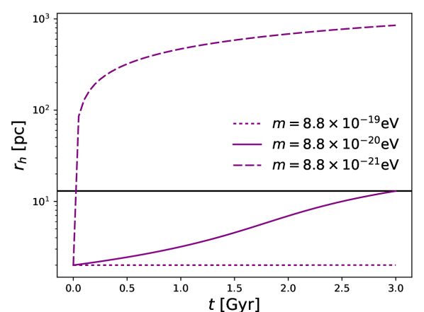
Figure 4: Expansion of the central star cluster of Eridanus II under the influence of fluctuations resulting from its embedding in a halo of FDM ultra-light axion dark matter of mass $m$. The horizontal line corresponds to the cluster’s estimated half mass radius.

Marsh & Niemeyer (2018) applied the model of El-Zant et al. (2016) to study the effect of FDM fluctuations on the central cluster of the dwarf galaxy Eridanus II. As the cluster’s embedding in a fluctuating FDM halo can cause it to expand, the idea was to place constraints on the ultra light axion mass from the observed size of the cluster, in analogy with what Brandt (2016) obtained for MACHOS. As the present work presents an extension and refinement of the model of El-Zant et al. (2016), with detailed application to the case of FDM haloes, it is of interest to revisit the case of Eridanus II in this context and examine its predictions.

As in Brandt (2016) and Marsh & Niemeyer (2018), we consider the central cluster to expand in virial equilibrium, keeping the same form of the density profile, as its stars gain kinetic energy due to its embedding in the fluctuating medium. The equation for the temporal evolution of the cluster’s half mass radius is then

$$\frac{dr_{h}}{dt}=\frac{D}{G}\left(\frac{\alpha M_{\star}}{r_{h}^{2}}+2\beta\rho_{0}r_{h}\right)^{-1},$$ (124)

where $D$ is the diffusion coefficient. As in the aforementioned work we adopt $\alpha=0.4$ and $\beta=10$, which corresponds to a cored Sérsic profile. The star cluster mass is taken to be $M_{\star}=2000M_{\odot}$. Here we concentrate on the case where the dark matter is composed solely of FDM. Furthermore, our model is strictly valid only outside the solitonic core, so the factor $\mathcal{CF}$ in equation (16) of Marsh & Niemeyer (2018) is unity (more on these issues below).

In the context of the present work, the diffusion coefficient is given in terms of equation (61); that is

$$D\left[(\Delta v)^{2}\right]=\frac{4\sqrt{2}\pi G^{2}\rho_{0}m_{\rm eff}}{\sigma_{\rm eff}}\ln\Lambda\left[\frac{{\rm erf}(X_{\rm eff})}{X_{\rm eff}}\right],$$ (125)

where $m_{\rm eff}$ is given by (59), $\sigma_{\rm eff}=\sigma/\sqrt{2}$ and $X_{\rm eff}=v_{p}/\sigma$. As in the previous appendix, we take the star cluster particle speed $v_{p}$ to correspond to the Keplerian velocity $v_{p}=0.83~{}{\rm km/s}\sqrt{{\rm 13pc}/R}$, and the dark matter velocity dispersion to be $\sigma=6.9~{}{\rm km/s}$. Thus, ${\rm erf}(X_{\rm eff})/X_{\rm eff}$ is about 1.1. The Coulomb logarithm is given by Eq. (123). Note that if the dark matter is not solely made of FDM, which instead only constitutes a fraction $\mathcal{F}$ (as assumed in Brandt, 2016 and Marsh & Niemeyer, 2018) the diffusion coefficient is effectively multiplied by a factor $\mathcal{F}^{2}$; as $\rho_{0}\rightarrow\mathcal{F}\rho_{0}$ and $m_{\rm eff}\rightarrow\mathcal{F}m_{\rm eff}$, since the latter also involves a factor $\rho_{0}$.

Fig. 4 shows the temporal evolution of the cluster’s radius over an assumed age of 3 Gyr from an assumed initial radius of $r_{h}=2~{}{\rm pc}$, which is the typical radius of stellar clusters in the Milky Way (e.g. Harris, 1996; Kharchenko et al., 2005). If the effect of FDM fluctuations is directed entirely at expanding the cluster, and if the current cluster radius is $13~{}{\rm pc}$, then the results suggest an FDM axion mass $m\geq 8.8\times 10^{-20}{\rm eV}$, which is essentially the same constraint as that obtained by Marsh & Niemeyer (2018) under the same assumptions regarding the FDM contribution to the dark matter, the cluster’s age and its initial and final sizes.

However, as pointed out by Marsh & Niemeyer (2018), the cluster lies inside the solitonic core for masses $m\la 10^{-20}{\rm eV}$. Strictly speaking neither the present formulation, or that of El-Zant et al. (2016) apply in this case. Indeed, in these contexts, the potential variations result from the existence of Gaussian random field of spatial fluctuations, transported into the time domain with mode velocity ${\bf v}$, rather than coherent core oscillations. Thus the constraints on the FDM axion mass appear limited in range. For, although Marsh & Niemeyer (2018) use a factor $\mathcal{C}$ (taken to be 0.3 inside the core) to take into account the effect of attenuated amplitudes of fluctuations due to core oscillations, and thus extend the constraint to smaller FDM masses for which the cluster lies inside the core, as Fig. 2 (upper panel) shows, the fluctuations close to the core also have much longer correlation times. This may render the random Gaussian assumption for the fluctuations, and the associated stochastic dynamics with a diffusion limit, more difficult to justify unless the timescales considered are sufficiently long. As mentioned in Section 3.2.1, incorporating the core oscillations would in addition require modification of the model to take into account the associated limited frequency range characterizing the oscillations.

These complications may not entirely eliminate the effect of core oscillations, and fluctuations from FDM granules outside the core can still affect the evolution of a cluster embedded inside it, and thus lead to strong constraints on $m$. However another caveat hinders direct extensions of the exclusion limits obtained above to small masses. Namely, for masses greater than $m=1.6\times 10^{-19}{\rm eV}$, the minimal wavelength associated with the size of the FDM quasi-particle granules is larger than the initial estimated characteristic cluster size: $\lambda_{\rm min}\leq 2{\rm pc}$. For $m\approx 10^{-20}{\rm eV}$ it is an order of magnitude larger. It is therefore unclear whether it is appropriate to consider that the associated fluctuations (or core oscillations) affect the internal structure of the cluster, as assumed above, rather than the cluster as a whole. If the latter situation is assumed, then for $m_{\rm eff}\gg M_{\star}$ one may expect energy equipartition between FDM quasi-particles and the cluster to result in significant motion of its centre of mass.

For example, for $m=10^{-20}{\rm eV}$, $m_{\rm eff}=1.8\times 10^{4}~{}M_{\odot}\gg M_{\star}$, which is an order of magnitude larger than the total cluster mass. The cluster should then gain random motion as a result of its embedding in the FDM ’heat bath’. Indeed, in that case, naive application of Eq. (62) leads one to deduce that the cluster gains a random velocity of order $\langle(\Delta v_{c})^{2}\rangle^{1/2}=24~{}{\rm km/s}$, which should displace it well outside the centre of the galaxy.

Such arguments, based on the cluster’s displacement form the centre of the galaxy, may thus in principle rule smaller out FDM axion masses, replacing the ones based on the cluster’s expansion. However, detailed examination of such issues, including the more complex intermediate mass case, are beyond the scope of this work.

References

- Amorisco & Loeb (2018) Amorisco N. C., Loeb A., 2018, arXiv e-prints, p. arXiv:1808.00464
- Arcadi et al. (2018) Arcadi G., Dutra M., Ghosh P., Lindner M., Mambrini Y., Pierre M., Profumo S., Queiroz F. S., 2018, European Physical Journal C, 78, 203
- Bar-Or et al. (2019) Bar-Or B., Fouvry J.-B., Tremaine S., 2019, ApJ, 871, 28
- Bar et al. (2019) Bar N., Blum K., Lacroix T., Panci P., 2019, arXiv e-prints, p. arXiv:1905.11745
- Binney & Tremaine (2008) Binney J., Tremaine S., 2008, Galactic dynamics
- Bode et al. (2001) Bode P., Ostriker J. P., Turok N., 2001, ApJ, 556, 93
- Bottema (1993) Bottema R., 1993, A&A, 275, 16
- Bournaud et al. (2009) Bournaud F., Elmegreen B. G., Martig M., 2009, ApJ, 707, L1
- Boveia & Doglioni (2018) Boveia A., Doglioni C., 2018, Annual Review of Nuclear and Particle Science, 68, annurev
- Brandt (2016) Brandt T. D., 2016, ApJ, 824, L31
- Bullock & Boylan-Kolchin (2017) Bullock J. S., Boylan-Kolchin M., 2017, Annual Review of Astronomy and Astrophysics, 55, 343
- Burkert (2000) Burkert A., 2000, ApJ, 534, L143
- Chan et al. (2018) Chan J. H. H., Schive H.-Y., Woo T.-P., Chiueh T., 2018, MNRAS, 478, 2686
- Chavanis (2011) Chavanis P.-H., 2011, Phys. Rev. D, 84, 043531
- Chavanis (2012) Chavanis P.-H., 2012, Physica A Statistical Mechanics and its Applications, 391, 3680
- Chavanis (2013) Chavanis P. H., 2013, A&A, 556, A93
- Chavanis (2018) Chavanis P.-H., 2018, arXiv e-prints
- Church et al. (2018) Church B. V., Ostriker J. P., Mocz P., 2018, arXiv e-prints, p. arXiv:1809.04744
- Cohen (1975) Cohen L., 1975, in Hayli A., ed., IAU Symposium Vol. 69, Dynamics of the Solar Systems. p. 33
- Cole et al. (2011) Cole D. R., Dehnen W., Wilkinson M. I., 2011, MNRAS, 416, 1118
- Colín et al. (2000) Colín P., Avila-Reese V., Valenzuela O., 2000, ApJ, 542, 622
- Crnojević et al. (2016) Crnojević D., Sand D. J., Zaritsky D., Spekkens K., Willman B., Hargis J. R., 2016, ApJ, 824, L14
- Davies & Mocz (2019) Davies E. Y., Mocz P., 2019, arXiv:1908.04790
- Davoudiasl & Denton (2019) Davoudiasl H., Denton P. B., 2019, arXiv e-prints, p. arXiv:1904.09242
- Del Popolo & Le Delliou (2017) Del Popolo A., Le Delliou M., 2017, Galaxies, 5, 17
- Del Popolo et al. (2014) Del Popolo A., Lima J. A. S., Fabris J. C., Rodrigues D. C., 2014, J. Cosmology Astropart. Phys., 4, 21
- Deng et al. (2018) Deng H., Hertzberg M. P., Namjoo M. H., Masoumi A., 2018, Phys. Rev. D, 98, 023513
- Desjacques & Nusser (2019) Desjacques V., Nusser A., 2019, arXiv e-prints, p. arXiv:1905.03450
- El-Zant et al. (2001) El-Zant A., Shlosman I., Hoffman Y., 2001, ApJ, 560, 636
- El-Zant et al. (2004) El-Zant A. A., Hoffman Y., Primack J., Combes F., Shlosman I., 2004, ApJ, 607, L75
- El-Zant et al. (2015) El-Zant A., Khalil S., Sil A., 2015, Phys. Rev. D, 91, 035030
- El-Zant et al. (2016) El-Zant A. A., Freundlich J., Combes F., 2016, MNRAS, 461, 1745
- Elbert et al. (2015) Elbert O. D., Bullock J. S., Garrison-Kimmel S., Rocha M., Oñorbe J., Peter A. H. G., 2015, MNRAS, 453, 29
- Frenk & White (2012) Frenk C. S., White S. D. M., 2012, Annalen der Physik, 524, 507
- Freundlich et al. (2019) Freundlich J., Dekel A., Jiang F., Ishai G., Cornuault N., Lapiner S., Dutton A. A., Maccio A. V., 2019, arXiv e-prints, p. arXiv:1907.11726
- Goerdt et al. (2010) Goerdt T., Moore B., Read J. I., Stadel J., 2010, ApJ, 725, 1707
- Goodman (2000) Goodman J., 2000, New Astron., 5, 103
- Governato et al. (2012) Governato F., et al., 2012, MNRAS, 422, 1231
- Harris (1996) Harris W. E., 1996, AJ, 112, 1487
- Heyvaerts (2010) Heyvaerts J., 2010, MNRAS, 407, 355
- Hu et al. (2000) Hu W., Barkana R., Gruzinov A., 2000, Physical Review Letters, 85, 1158
- Hui et al. (2017) Hui L., Ostriker J. P., Tremaine S., Witten E., 2017, Phys. Rev. D, 95, 043541
- Kharchenko et al. (2005) Kharchenko N. V., Piskunov A. E., Röser S., Schilbach E., Scholz R. D., 2005, A&A, 438, 1163
- Kobayashi et al. (2017) Kobayashi T., Murgia R., De Simone A., Iršič V., Viel M., 2017, Phys. Rev. D, 96, 123514
- Kochanek & White (2000) Kochanek C. S., White M., 2000, ApJ, 543, 514
- Kraichnan (1964) Kraichnan R. H., 1964, Physics of Fluids, 7, 1723
- Kregel & van der Kruit (2005) Kregel M., van der Kruit P. C., 2005, MNRAS, 358, 481
- Kregel et al. (2005) Kregel M., van der Kruit P. C., Freeman K. C., 2005, MNRAS, 358, 503
- Kubo (1966) Kubo R., 1966, Reports on Progress in Physics, 29, 255
- Lacey & Ostriker (1985) Lacey C. G., Ostriker J. P., 1985, ApJ, 299, 633
- Lee (2018) Lee J.-W., 2018, in European Physical Journal Web of Conferences. p. 06005 (arXiv:1704.05057), doi:10.1051/epjconf/201816806005
- Li et al. (2017) Li T. S., et al., 2017, ApJ, 838, 8
- Lidz & Hui (2018) Lidz A., Hui L., 2018, Phys. Rev. D, 98, 023011
- Lin et al. (2018) Lin S.-C., Schive H.-Y., Wong S.-K., Chiueh T., 2018, Phys. Rev. D, 97, 103523
- Lovell et al. (2014) Lovell M. R., Frenk C. S., Eke V. R., Jenkins A., Gao L., Theuns T., 2014, MNRAS, 439, 300
- Macciò et al. (2012) Macciò A. V., Paduroiu S., Anderhalden D., Schneider A., Moore B., 2012, MNRAS, 424, 1105
- Mackereth et al. (2019) Mackereth J. T., et al., 2019, arXiv e-prints, p. arXiv:1901.04502
- Madau et al. (2014) Madau P., Shen S., Governato F., 2014, ApJ, 789, L17
- Marsh (2016) Marsh D. J. E., 2016, Phys. Rep., 643, 1
- Marsh (2017) Marsh D. J. E., 2017, arXiv e-prints, p. arXiv:1712.03018
- Marsh & Niemeyer (2018) Marsh D. J. E., Niemeyer J. C., 2018, arXiv e-prints, p. arXiv:1810.08543
- Marsh & Silk (2014) Marsh D. J. E., Silk J., 2014, MNRAS, 437, 2652
- Martínez & Saar (2002) Martínez V. J., Saar E., 2002, Statistics of the Galaxy Distribution. Chapman
- Martizzi et al. (2013) Martizzi D., Teyssier R., Moore B., 2013, MNRAS, 432, 1947
- Mashchenko et al. (2006) Mashchenko S., Couchman H. M. P., Wadsley J., 2006, Nature, 442, 539
- Mashchenko et al. (2008) Mashchenko S., Wadsley J., Couchman H. M. P., 2008, Science, 319, 174
- Miralda-Escudé (2002) Miralda-Escudé J., 2002, ApJ, 564, 60
- Mo et al. (2010) Mo H., van den Bosch F. C., White S., 2010, “Galaxy Formation and Evolution”
- Mocz et al. (2019) Mocz P., et al., 2019, Phys. Rev. Lett., 123, 141301
- Navarro et al. (1996) Navarro J. F., Frenk C. S., White S. D. M., 1996, ApJ, 462, 563
- Nebrin et al. (2018) Nebrin O., Ghara R., Mellema G., 2018, arXiv e-prints, p. arXiv:1812.09760
- Nipoti & Binney (2015) Nipoti C., Binney J., 2015, MNRAS, 446, 1820
- Nori et al. (2019) Nori M., Murgia R., Iršič V., Baldi M., Viel M., 2019, MNRAS, 482, 3227
- Osterbrock (1952) Osterbrock D. E., 1952, ApJ, 116, 164
- Peebles (2000) Peebles P. J. E., 2000, ApJ, 534, L127
- Peirani et al. (2008) Peirani S., Kay S., Silk J., 2008, A&A, 479, 123
- Peter et al. (2013) Peter A. H. G., Rocha M., Bullock J. S., Kaplinghat M., 2013, MNRAS, 430, 105
- Pontzen & Governato (2012) Pontzen A., Governato F., 2012, MNRAS, 421, 3464
- Pontzen & Governato (2014) Pontzen A., Governato F., 2014, Nature, 506, 171
- Read & Gilmore (2005) Read J. I., Gilmore G., 2005, MNRAS, 356, 107
- Robles et al. (2019) Robles V. H., Bullock J. S., Boylan-Kolchin M., 2019, MNRAS, 483, 289
- Romano-Díaz et al. (2008) Romano-Díaz E., Shlosman I., Hoffman Y., Heller C., 2008, ApJ, 685, L105
- Roszkowski et al. (2018) Roszkowski L., Sessolo E. M., Trojanowski S., 2018, Reports on Progress in Physics, 81, 066201
- Ruffini & Bonazzola (1969) Ruffini R., Bonazzola S., 1969, Physical Review, 187, 1767
- Safarzadeh & Spergel (2019) Safarzadeh M., Spergel D. N., 2019, arXiv e-prints, p. arXiv:1906.11848
- Schive et al. (2014a) Schive H.-Y., Chiueh T., Broadhurst T., 2014a, Nature Physics, 10, 496
- Schive et al. (2014b) Schive H.-Y., Liao M.-H., Woo T.-P., Wong S.-K., Chiueh T., Broadhurst T., Hwang W.-Y. P., 2014b, Physical Review Letters, 113, 261302
- Schneider et al. (2012) Schneider A., Smith R. E., Macciò A. V., Moore B., 2012, MNRAS, 424, 684
- Shao et al. (2013) Shao S., Gao L., Theuns T., Frenk C. S., 2013, MNRAS, 430, 2346
- Spergel & Steinhardt (2000) Spergel D. N., Steinhardt P. J., 2000, Physical Review Letters, 84, 3760
- Taylor (1938) Taylor G. I., 1938, Proceedings of the Royal Society of London A: Mathematical, Physical and Engineering Sciences, 164, 476
- Tennekes (1975) Tennekes H., 1975, Journal of Fluid Mechanics, 67, 561
- Teyssier et al. (2013) Teyssier R., Pontzen A., Dubois Y., Read J. I., 2013, MNRAS, 429, 3068
- Tonini et al. (2006) Tonini C., Lapi A., Salucci P., 2006, ApJ, 649, 591
- Veltmaat et al. (2018) Veltmaat J., Niemeyer J. C., Schwabe B., 2018, Phys. Rev. D, 98, 043509
- Vincenzo et al. (2019) Vincenzo F., Kobayashi C., Yuan T., 2019, MNRAS, 488, 4674
- Wasserman et al. (2019) Wasserman A., et al., 2019, arXiv e-prints, p. arXiv:1905.10373
- Weinberg (1993) Weinberg M. D., 1993, ApJ, 410, 543
- Wilczek & Narita (2012) Wilczek M., Narita Y., 2012, Phys. Rev. E, 86, 066308
- Wilczek et al. (2014) Wilczek M., Xu H., Narita Y., 2014, Nonlinear Processes in Geophysics, 21, 645
- Zavala et al. (2013) Zavala J., Vogelsberger M., Walker M. G., 2013, MNRAS, 431, L20
- Zolotov et al. (2012) Zolotov A., et al., 2012, ApJ, 761, 71