Consistent Classification with Generalized Metrics

Abstract

We propose a framework for constructing and analyzing multiclass and multioutput classification metrics i.e., involving multiple, possibly correlated multiclass labels. Our analysis reveals novel insights on the geometry of feasible confusion tensors – including necessary and sufficient conditions for the equivalence between optimizing an arbitrary non-decomposable metric and learning a weighted classifier. Further, we analyze averaging methodologies commonly used to compute multioutput metrics and characterize the corresponding Bayes optimal classifiers. We show that the plug-in estimator based on this characterization is consistent and is easily implemented as a post-processing rule. Empirical results on synthetic and benchmark datasets support the theoretical findings.

1 Introduction

Learning with weighted losses is known to be a population optimal classification strategy (equiv. Bayes optimal) for a wide variety of performance metrics. For instance, weighted losses can be used to estimate Bayes optimal classifiers for binary classification with linear or fractional-linear metrics such as weighted accuracy and F-measure [12], multiclass classification with linear, concave or fractional linear metrics such as weighed accuracy and ordinal loss [17], and multilabel classification with averaged linear and fractional-linear metrics [13].

Perhaps due to these theoretical results and evident practical success, learning using weighted losses is a popular strategy for constructing predictive models when attempting to optimize complex classification metrics. Unfortunately, it is not known in general when the weighted classifier strategy is a convenient heuristic vs. when it results in provably consistent classifiers. This gap in the literature motivates the question, when is classification with weighted losses provably consistent? We provide an answer by characterizing necessary and sufficient conditions under which learning with weighted losses can recover population optimal classifiers. Interestingly, our results justify the use of weighted losses for many practical settings. For instance, we recover known results that monotonic metrics and fractional-linear metrics satisfy the necessary and sufficient conditions, and thus are optimized by the weighted classifier.

Beyond binary, multiclass and multilabel classification, multioutput learning, also variously known as multi-target, multi-objective, multi-dimensional learning, is the supervised learning problem where each instance is associated with multiple target variables[20, 25]. Formalizing predictive problems in this way has led to empirical success in applied areas like natural language processing [24] and computer vision [8, 31], where combining different tasks boosts the performance of each individual class. For example, in a movie recommendation system, the learner must predict discrete user ratings for multiple movies simultaneously. In natural language processing, one can learn the POS tagging, chunking, and dependency parsing jointly [7]. In this manuscript, we aim to provide a theoretical understanding of multioutput classification problems i.e. where all outputs are discrete.

In particular, Bayes optimal and consistent classifiers for multioutput classifiers have so far remained unexplored. To this end, another goal of this manuscript is to characterize Bayes optimal multioutput classifiers for a broad range of metrics.

Perhaps the most popular approach for constructing multioutput classifiers in practice is by averaging multiclass metrics. Interestingly, this mirrors the popularity of averaged binary metrics for multilabel classification [13]. Averaged multiclass metrics are constructed by averaging with respect to examples separately for each output (macro-averaging), or with respect to both outputs and examples (micro-averaging). For such averaged metrics, when the classifier is given by a function of the confusion matrix, we characterize both necessary and sufficient conditions for the Bayes optimal classifier to be given by a simple weighted classifier – specifically, the deterministic classifier which minimizes a weighted loss. We note that this result holds even when the outputs are highly correlated. Further, we show that the associated weights are shared by all the outputs when the metric is micro-averaged. Taken together, these results clarify the role of output correlations in averaged multioutput classification.

The family of fractional linear metrics is of special interest, as examples in this family include widely used metrics such as the multioutput averaged F-measure, among others. For fractional linear metrics, we propose a simple plug-in estimator that can be implemented as a post-processing rule (equiv. as a weighted classifier). We show that this plug-in classifier is consistent i.e. the population utility of the empirical estimator approaches the utility of the Bayes classifier with large samples. We also present experimental evaluation on synthetic and real-world benchmark datasets and a movie recommendation dataset comparing different estimation algorithms. The empirical results show that the proposed approach leads to improved classifiers in practice.

Main contributions:

1. We characterize necessary and sufficient conditions which determine when weighted classification results in a Bayes optimal multioutput classification. Our characterization recovers recent results on sufficient conditions for binary, multiclass, and multilabel classification.

2. We show that even when labels are correlated, under standard assumptions, the Bayes optimal multioutput classifier decomposes across outputs.

3. We propose a plug-in estimator for averaging of fractional-linear class performance metrics, and provide a thorough empirical evaluation. Further, we empirically analyze conditions where using the Bayes optimal procedure may be helpful and other cases where its use may not affect performance – thus providing practical guidance.

1.1 Related Work

Perhaps due to increasing applied interest in complex classification metrics for specialized applications, there is a growing literature on the analysis and practical implementation of consistent classifiers.  Koyejo et al. [12] discuss consistent binary classifiers for generic ratios of linear metrics.  Tewari and Bartlett [26] showed that multiclass classifiers constructed using consistent binary classifiers may still lead to inconsistent multiclass results.  Narasimhan et al. [17] further propose consistent multiclass classifiers for both concave and fractional-linear metrics.  Osokin et al. [18] consider structured prediction with convex surrogate losses for decompose multiclass classification metrics (i.e. metrics that can be expressed as an average over samples).

Studies of multilabel classification [5, 3] compare separate (label-wise independent) classification to a variety of correlated label approaches for optimizing hamming loss, showing that separate classification is often competitive.  Dembczyński et al. [4] also critically highlight how the same multilabel classifier may not be optimal for different loss functions – thus, classifiers must be appropriately tuned to metrics of interest. Koyejo et al. [13] reveal a parametric form for population optimal multilabel classifiers which can be decomposed to binary classifiers and explore efficient algorithms for fractional of linear metrics. We note that consistent binary, multiclass and multilabel classification are special cases of consistent multioutput classification.

While the multioutput problem is ubiquitous, much of the literature focuses on algorithms and applications – and few (if any) prior work has considered consistency to the best of our knowledge.

One line of work proposes new algorithms for multioutput problems, most of which are designed to model the correlation relationships between the labels. Examples include the Bayesian chain classifier [30, 29], classifier trellises [21], and general graphical models [24] among others.

Read et al. [19] address the multioutput classification problem using what they call the multidimensional Bayesian network classifiers (MBCs). However, the only metric they consider is the 0-1 loss. Borchani et al. [1] further propose a Markov blanket-based approach to train the MBCs from multioutput data. Saha et al. [25] formulate the multitask multilabel framework to make predictions on data from Electronic Medical Records, and solve the iterative optimization problem by block co-ordinate descent. Read et al. [20] solve the multi-dimensional (multioutput) classification problem by modeling label dependencies.

2 Problem Setup and Notation

Consider the multioutput classification problem where $\mathcal{X}$ denotes the instance space and $\mathcal{Y}=\left[K\right]^{M}$ denotes the output space with $M$ outputs and $K$ classes per output. Without loss of generality, we assume that the number of classes is the same for all outputs, i.e. $K_{m}=K$ for $m=1,\dots,M$. If the numbers of classes are different for each output, we can simply set $K=\max_{m}K_{m}$ i.e. padding classes with null labels as required. We provide several such examples in practice in Section 5. Assume the instances and outputs follow some probability distribution $\mathbb{P}$ over the domain $\mathcal{X}\times\mathcal{Y}$. A dataset is given by $N$ samples $(x^{(i)},\mathbf{y}^{(i)})\overset{\text{i.i.d}}{\sim}\mathbb{P},i\in[N]$. Since $\mathbb{P}$ is general, the outputs could be highly correlated across outputs.

Define the set of randomized classifiers $\mathcal{H}_{r}=\{\mathbf{h}:\mathcal{X}\to(\Delta^{K})^{M}\}$, where $\Delta^{q}=\left\{\mathbf{p}\in[0,1]^{q}:\sum_{i=1}^{q}p_{i}=1\right\}$ is the $q-1$ dimensional probability simplex. For any multioutput classifier, we can define the confusion tensor as follows. Assume $\mathbf{h}\in\mathcal{H}_{r}$, and the prediction for the $m$th output is $h_{m}(\cdot)\in\mathbb{R}^{K}$. Let $\mathbf{\bm{\eta}}(x)\in\mathbb{R}^{K\times M}$ denote the marginal class probability for any given instance $x$, whose $(k,m)$th element is the conditional probability of output $m$ belonging to class $k$: $\eta^{m}_{k}(x)=\mathbb{P}(Y_{m}=k\mid X=x)$. The population confusion tensor is $\mathbf{\bm{C}}\in[0,1]^{M\times K\times K}$, with elements are defined as

$$\mathbf{\bm{C}}_{m,k,\ell}=\int_{x}h^{m}_{k}(x)\mathbf{\bm{\eta}}^{m}_{\ell}(x)d\mathbb{P}(x),$$ (1)

or equivalently, $\mathbf{\bm{C}}_{m,k,\ell}=\mathbb{P}(h^{m}_{k}(x)=1,Y_{m}=\ell)$.

The sample confusion tensor is defined as $\mathbf{\bm{\widehat{C}}}(\mathbf{\bm{h}})=\frac{1}{N}\sum_{n=1}^{N}\mathbf{\bm{\widehat{C}}}^{(n)}(\mathbf{\bm{h}})$, where $\mathbf{\bm{\widehat{C}}}^{(n)}(\mathbf{\bm{h}})\in\{0,1\}^{M\times K\times K}$, and $\widehat{C}_{m,i,j}^{(n)}(\mathbf{\bm{h}})=\left\llbracket y_{m}^{(n)}=i,h_{m}(x^{(n)})=j\right\rrbracket$. Here $\left\llbracket\cdot\right\rrbracket$ is the indicator function, so $\sum_{i=1}^{K}\sum_{j=1}^{K}\widehat{C}_{m,i,j}^{(n)}(\mathbf{\bm{h}})=1$. For $\mathbf{h}\in\mathcal{H}_{r}$, due to the linearity of confusion tensor definition, we have $\mathbf{\bm{\widehat{C}}}^{(n)}(\mathbf{\bm{h}})\in\left[0,1\right]^{M\times K\times K}$. Note that for multiclass classification with a single output, the confusion tensor reduces to a $K\times K$ matrix, commonly simply known as the confusion matrix.

Performance Metrics

We consider the general class of performance metrics $\mathcal{U}_{\Psi}:\mathcal{H}\mapsto\mathbb{R}_{+}$ for multioutput problems, which can be represented as a function of the confusion tensor, i.e. $\mathcal{U}_{\Psi}(\mathbf{h})=\Psi(\mathbf{\bm{C}}(\mathbf{h}))$. This setting has been studied in binary classification [27], multiclass classification [17] and multilabel classification [14].

The goal is to learn the Bayes classifier with respect to the given metric:

$$\mathbf{\bm{h}}^{*}_{\Psi}\in\operatorname*{argmax}_{\mathbf{\bm{h}}}\;\mathcal{U}_{\Psi}(\mathbf{\bm{h}}).$$

We denote the optimal utility as $\mathcal{U}^{*}_{\Psi}=\mathcal{U}_{\Psi}(\mathbf{\bm{h}}^{*}_{\Psi})$. We say a classifier $\mathbf{\bm{h}}_{N}$ constructed using finite data of size $N$ is $\Psi$-consistent if $\mathcal{U}_{\Psi}(\mathbf{\bm{h_{N}}})\xrightarrow{\mathbb{P}}\mathcal{U}^{*}_{\Psi}$. And to measure the non-asymptotic performance of a learned classifier, we define regret as follows.

Definition 1

($\Psi$-regret). For any classifier $\mathbf{h}$ and a function $\Psi$: $\left[0,1\right]^{M\times K\times K}\to\mathbb{R}_{+}$, define a $\Psi$-regret of $\mathbf{h}$ w.r.t. distribution $\mathbb{P}$ as the difference between its $\Psi$-performance and the optimal: $\mathcal{U}^{*}_{\Psi,\mathbb{P}}-\mathcal{U}_{\Psi,\mathbb{P}}(\mathbf{h}).$

Notation

Throughout the paper, we use uppercased bold letters to represent tensors and matrices, and lowercased bold letters to represent vectors. Let $e_{i}$ represent the $i$th standard basis whose $i$th dimension is 1 and 0 otherwise $e_{i}=(0,\cdots,1,\cdots,0)$. We follow the tensor computation notation of Kolda and Bader [10]. For an order-$P$ tensor $\mathbf{\bm{A}}\in\mathbb{R}^{D_{1}\times\cdots\times D_{P}}$, we use $A_{i_{1},\dots,i_{P}}$ to represent its elements, where $i_{p}\in[D_{p}]$ for $p=1,\dots,P$; and $\mathbf{\bm{A}}_{\cdot,\cdot,\cdots,i_{p},\cdots,\cdot}$ to represent the $i_{p}$th mode-$D$ slice of $\mathbf{\bm{A}}$, which is a $P-1$ dimensional tensor obtained by fixing the $p$th index to be $i_{p}$. For two tensors $\mathbf{\bm{A}},\mathbf{\bm{B}}$ of the same dimension, we define their inner product as the sum of element-wise product over all corresponding positions, i.e., $\left\langle\mathbf{\bm{A}},\mathbf{\bm{B}}\right\rangle=\sum_{i_{1}=1}^{D_{1}}\cdots\sum_{i_{P}=1}^{N_{P}}A_{i_{1},\cdots,i_{P}}B_{i_{1},\cdots,i_{P}}$. The $D$-mode (vector) product of a tensor $\mathbf{\bm{A}}\in\mathbb{R}^{D_{1},\cdots,D_{j-1},D_{j},D_{j+1}\cdots,D_{P}}$ with a vector $\mathbf{\bm{u}}\in\mathbb{R}^{D_{j}}$ is denoted by $A\mathchoice{\mathbin{\vbox{\hbox{\scalebox{1.0}{$\displaystyle\bullet$}}}}}{\mathbin{\vbox{\hbox{\scalebox{1.0}{$\textstyle\bullet$}}}}}{\mathbin{\vbox{\hbox{\scalebox{1.0}{$\scriptstyle\bullet$}}}}}{\mathbin{\vbox{\hbox{\scalebox{1.0}{$\scriptscriptstyle\bullet$}}}}}_{j}\mathbf{\bm{u}}$. The result is of order $P-1$ with size $D_{1}\times\cdots\times D_{j-1}\times D_{j+1}\times\cdots\times D_{P}$. Element-wise,

$$(A\mathchoice{\mathbin{\vbox{\hbox{\scalebox{1.0}{$\displaystyle\bullet$}}}}}{\mathbin{\vbox{\hbox{\scalebox{1.0}{$\textstyle\bullet$}}}}}{\mathbin{\vbox{\hbox{\scalebox{1.0}{$\scriptstyle\bullet$}}}}}{\mathbin{\vbox{\hbox{\scalebox{1.0}{$\scriptscriptstyle\bullet$}}}}}_{j}\mathbf{\bm{u}})_{i_{1},\cdots,i_{j-1},i_{j+1},\cdots,i_{P}}=\sum_{k=1}^{D_{j}}A_{i_{1},\cdots,i_{j-1},k,i_{j+1},\cdots,i_{P}}\mathbf{\bm{u}}_{k}$$

We use $\otimes$ to represent the outer product between vectors or tensors.

3 Bayes Optimal Multioutput Classifiers

In this section, we characterize the conditions for defining a Bayes optimal classifier under general performance metrics.

3.1 Properties of Confusion Tensors

We consider the properties of the classifiers in the confusion tensor space. First, we define the set of feasible confusion tensors for all feasible classifiers.

Definition 2 (Feasible Confusions)

Given the distribution $\mathbb{P}$, Let $\mathbf{\bm{C}}(\mathbf{\bm{h}})=\mathbb{E}{[\hat{\mathbf{\bm{C}}}(\mathbf{\bm{h}})]}$ denote the population confusion. The set of all feasible population confusions is given by: $\mathcal{C}=\left\{\mathbf{\bm{C}}(\mathbf{\bm{h}})\mid\mathbf{h}\in\mathcal{H}_{r}\right\}$.

By the linearity of the confusion tensor, we have the following.

Lemma 1 (Convexity and compactness)

The set $\mathcal{C}$ is convex and compact.

The existence of an optimal classifier follows from the compactness and the convexity of $\mathcal{C}$. The Bayes confusion matrix corresponding to the utility $\mathcal{U}_{\Psi}(\mathbf{h})$ is denoted by $\mathbf{\bm{C}}^{*}=\mathbf{\bm{C}}(\mathbf{\bm{h}}^{*}_{\Psi})=\max_{\mathbf{\bm{C}}}\Psi(\mathbf{\bm{C}})$. Moreover, we have the following property of the optimal confusion tensor.

Lemma 2

Let $\mathcal{C}$ be the set of feasible confusions with boundary $\partial\mathcal{C}$. If $\mathbf{\bm{C}}^{*}\in\partial\mathcal{C}$, then there exists $\mathbf{\bm{L}}\in\mathbb{R}^{M\times K\times K}$ such that $\mathbf{\bm{C}}^{*}\in\arg\min_{\mathbf{\bm{C}}}\left\langle\mathbf{\bm{L}},\mathbf{\bm{C}}\right\rangle$.

In other words, optimizing any metric that satisfies $\mathbf{\bm{C}}^{*}\in\partial\mathcal{C}$ can be reduced in maximizing a weighed loss. Thus, we state that any utility which satisfies $\mathbf{\bm{C}}^{*}\in\arg\min_{\mathbf{\bm{C}}}\left\langle\mathbf{\bm{L}},\mathbf{\bm{C}}\right\rangle$ for some $\mathbf{\bm{L}}$ admits a weighted Bayes optimal (we will define this formally in the sequel). Importantly, we note that $\mathbf{\bm{L}}$ is not unique, since the optimization is invariant to global scale and global additive constants. In the sequel, will usually assume $\left\lVert\mathbf{\bm{L}}\right\rVert=1$ for some norm $\left\lVert\cdot\right\rVert$.

On the other hand, we claim that if the Bayes optimal follows a weighted form, then the optimal confusion tensor necessarily lies on the boundary of the feasible set.

Lemma 3

If the utility function admits a weighted Bayes optimal i.e. $\exists\,\mathbf{\bm{L}}$ such that $\mathbf{\bm{C}}^{*}\in\arg\min_{\mathbf{\bm{C}}}\left\langle\mathbf{\bm{L}},\mathbf{\bm{C}}\right\rangle$ then the Bayes optimal confusion $\mathbf{C}^{*}\in\partial\mathcal{C}$.

Taken together, Lemma 2 and Lemma 3 characterize necessary and sufficient conditions for the Bayes optimality of weighted classifiers. For specific classes of metrics, the loss tensor can be characterized in closed-form.

Definition 3 (Monotonic Metrics)

A metric $\Psi$ is strictly monotonic if $\,\forall\,m\in[M]$, $\Psi$ is non-decreasing with respect to all elements of $\{\mathbf{\bm{C}}_{m,i,i}\mid i\in[K]\}$ and non-increasing with respect to all elements of $\{\mathbf{\bm{C}}_{m,i,j}\mid i,j\in[K]\}$.

Monotonic metrics are ubiquitous, as they capture the intuition that the utility should reward better performance and penalize worse performance (as measured by the confusion entries). To our knowledge, all classification metrics in common use satisfy monotonicity. For monotonic and differentiable metrics, we can characterize the loss tensor by the negative gradient of $\Psi$ at the optimal confusion tensor.

Lemma 4 (Optimal confusion tensor for monotonic and differentiable metric function)

Let $\Psi$ be a monotonic and differentiable metric, and $\mathbf{\bm{C}}^{*}=\mathbf{\bm{C}}(\mathbf{h}^{*}_{\Psi})$. Then $\mathbf{\bm{C}}^{*}\in\max_{\mathbf{\bm{C}}}\left\langle\nabla\Psi(\mathbf{\bm{C}}^{*}),\mathbf{\bm{C}}\right\rangle$.

Thus, without loss of generality, we can fix the loss matrix for monotonic and differentiable metrics as $\mathbf{\bm{L}}=1-\nabla\Psi(\mathbf{\bm{C}}^{*})$. Note that $\nabla\Psi(\mathbf{\bm{C}}^{*})$ does not depend on $\mathbf{\bm{C}}^{*}$ for weighted losses such as 0-1 loss (i.e. accuracy), thus can be calculated in closed form. While the Bayes optimal is a weighted classifier, obtaining the loss tensor is sometimes non-trivial. We propose an iterative algorithm in Section 4.

Finally, we also note that as a straightforward consequence of convexity of the feasible set, every confusion matrix can be computed as a mixture of two boundary points; thus all Bayes optimal classifiers can be expressed as a mixture of two weighted classifiers. This straightforward corollary is stated more formally without proof.

Corollary 1 (All Bayes Optima)

Any Bayes optimal confusion $\mathbf{C}^{*}\in\mathcal{C}$ can be expressed as the mixture of two weighted confusion matrices $\mathbf{C}^{*}=\alpha\mathbf{C}_{1}+(1-\alpha)\mathbf{C}_{2},$ where $\alpha\in[0,1]$ and $\mathbf{\bm{C}}_{i}\in\arg\min_{\mathbf{\bm{C}}}\left\langle\mathbf{\bm{L}}_{i},\mathbf{\bm{C}}\right\rangle$ for some $\{\mathbf{\bm{L}}_{1},\mathbf{\bm{L}}_{2}\}.$

3.2 Weighted Bayes Optimal Classifiers

The results in Section 3.1 are concerned only with the confusion tensor, and do not enforce any assumption on the classifier or the data distribution. When the joint distribution of the data is well-behaved, we can extend the optimization over confusion tensors into optimization over the corresponding classifiers. We introduce the following assumption on the joint distribution of the data.

Assumption 1

Assume $\mathbb{P}(\{\mathbf{\bm{\eta}}^{m}(X)=\mathbf{c}\})=0\;\forall\mathbf{c}\in\Delta^{K},\;m\in[M]$. Furthermore, let $Z^{m}=\mathbf{\bm{\eta}}^{m}(X)$ with density $p_{\eta}(Z^{m})$. For all $m\in[M]$, $p_{\eta}(Z^{m})$ is absolutely continuous with respect to the Lebesgue measure restricted to $\Delta^{K}$.

Analogous regularity assumptions are widely employed in literature on designing well-defined complex classification metrics and seem to be unavoidable (we refer interested reader to [27, 17] for details). The Bayes optimal classifier for linear multioutput metrics takes a particularly simple form.

Definition 4

We say a metric $\mathcal{U}_{\Psi}(\mathbf{h})$ admits a weighted Bayes optimal classifier $\mathbf{h}^{*}$ if there exists a loss tensor $\mathbf{\bm{L}}\in\mathbb{R}^{M\times K\times K}$, such that $\mathbf{h}^{*m}(x)=e_{\left\llbracket k=\arg\min_{k}\left\langle\mathbf{\bm{L}}_{k\cdot m},\mathbf{\bm{\eta}}^{m}\right\rangle\right\rrbracket}.$

Theorem 3.1

Under Assumption 1, when the metric $\mathcal{U}_{\Psi}(\mathbf{h})$ admits a weighted Bayes optimal (Definition 4), $\exists$ a Bayes optimal classifier $\mathbf{h}^{*}$ which satisfies $\mathbf{h}^{*m}(x)=e_{\left\llbracket k=\arg\min_{k}\left\langle\mathbf{\bm{L}}_{k\cdot m},\mathbf{\bm{\eta}}^{m}\right\rangle\right\rrbracket}$, where $\mathbf{\bm{L}}$ is as defined in Lemma 2.

Theorem 3.1 states that the correlation between outputs are fully reflected in the conditional probability. It unifies some known results: when $M=1$, this recovers the multiclass optimal result in [17]; when $K=2$, this recovers the multilabel results studied in [14]; when $M=1,K=2$, one can show that the weighted classifier reduces to standard thresholding for binary classification [27, 12].

Interestingly, Theorem 3.1 combined with Corollary 2 suggests a remarkable simplicity of all Bayes optimal classifiers, namely that either there exists a deterministic Bayes classifier, or there exists a Bayes classifier given by a mixture of two deterministic classifiers. This observation is stated more formally in the following corollary.

Corollary 2 (All Bayes Classifiers)

Under Assumption 1, for any metric $\mathcal{U}_{\Psi}(\mathbf{h})$, $\exists$ a Bayes optimal classifier $\mathbf{h}^{*}$ which satisfies $\mathbf{h}^{*}=\alpha\mathbf{h}_{1}+(1-\alpha)\mathbf{h}_{2}$, where $\mathbf{h}_{i}$ are weighted deterministic classifiers (Theorem 3.1), and $\mathbf{C}_{1}=\mathbf{C}(\mathbf{h}_{1})$, $\mathbf{C}_{2}=\mathbf{C}(\mathbf{h}_{2})$, $\mathbf{C}(\mathbf{h^{*}})=\mathbf{C}^{*}=\alpha\mathbf{C}_{1}+(1-\alpha)\mathbf{C}_{2}$ as defined in Corollary 2.

The theorem is a straightforward consequence of Corollary 2, and the observation that by definition, $\mathbf{C}_{i}$ admit a weighted Bayes optimal. Notably the same mixture weight $\alpha$ is optimal point-wise. The special case of deterministic classifiers (Theorem 3.1) is recovered when $\alpha=0$.

3.3 Averaged Multioutput Metrics and their Bayes Optima

The most common technique for constructing multioutput metrics is by treating each output as separate multiclass problem and averaging the corresponding multiclass performance metrics. Here we distinguish two types of averaging and discuss differences in their population behavior. For both averaging methods, we assume there exists a multiclass performance metric $\psi:[0,1]^{K\times K}\to\mathbb{R}$, and an output-specific weight vector $\mathbb{\alpha}\in\mathbb{R}^{M}$.

Microaveraging

Micro-averaging is implemented by averaging the multiclass confusion matrices for each output, then applying the performance function on the averaged confusion matrix. Formally,

$$\Psi_{\text{micro}}(\mathbf{\bm{\hat{C}}})=\psi\left(\sum_{m=1}^{M}\mathbb{\alpha}_{m}\hat{\mathbf{\bm{C}}}_{m\cdot\cdot}\right)=\psi\left(\frac{\mathbb{\alpha}_{m}}{N}\sum_{m=1}^{M}\sum_{n=1}^{N}\widehat{C}_{m,i,j}^{(n)}(h_{m})\right)$$

Macroaveraging

Macro-averaging is implemented by first applying the performance function $\psi$ to each output confusion matrix, then averaging over the outputs. Formally,

$$\Psi_{\text{macro}}(\mathbf{\bm{\hat{C}}})=\sum_{m=1}^{M}\mathbb{\alpha}_{m}\psi\left(\hat{\mathbf{\bm{C}}}_{m\cdot\cdot}\right)=\sum_{m=1}^{M}\mathbb{\alpha}_{m}\psi\left(\frac{1}{N}\sum_{n=1}^{N}\widehat{C}_{m,i,j}^{(n)}(h_{m})\right).$$

Examples of macro-averaged metrics include Decathlon score used by [22], where $\psi(C_{m\cdot\cdot})=1-\text{diag}(C_{m\cdot\cdot})$. Micro-averaging and Macro-averaging result in identical performance metrics for the case of linear functions $\psi$, such as those used in weighted average accuracy. Yet it will not be surprising these two types of averaging methodology result in different optimal classifiers for general non-linear functions $\psi$. Examples include linear metrics like Ordinal [17], Micro-$F_{1}$ [9] and Macro-$F_{1}$ [15]; weighted accuracy puts an exponential weights to each class; and polynomial functions are used in metrics such as Decathlon score [22]. Table 1 lists several examples of $\psi$ commonly used by practitioners in multiclass and multioutput classification.

Table 1: Examples of multiclass performance metrics

Performance Metrics	$\psi(\mathbf{\bm{C}})$
Ordinal	$\sum_{i=1}^{K}\sum_{j=1}^{K}(1-\frac{1}{n-1}\lvert i-j\rvert)C_{i,j}$
Micro-$F_{1}$	$\frac{2\sum_{i=2}^{K}C_{i,i}}{2-\sum_{i=1}^{K}C_{1,i}-\sum_{i=1}^{K}C_{i,1}}$
Macro-$F_{1}$	$\frac{1}{K}\sum_{i=1}^{K}\frac{2C_{i,i}}{\sum_{j=1}^{K}C_{i,j}+\sum_{j=1}^{K}C_{j,i}}$
Weightedγ	$\sum_{i=1}^{K}e^{-\gamma i}C_{ii}$
Min-max	$\min_{i\in\left[K\right]}\frac{C_{i,i}}{\sum^{n}_{j=1}C_{i,j}}$
Polynomial	$(1-\text{diag}(\mathbf{\bm{C}}))^{\gamma}$

The following propositions state some differences between the two kinds of averaging.

Proposition 1 (Shared Loss for micro-averaged metrics)

For micro-averaged multioutput metrics, all outputs (considered as multiclass problems) share the same loss matrix $\mathbf{\bm{L}}^{*}_{m\cdot\cdot}=\mathbf{\bm{S}},\,\forall\,m\in[M]$.

Now, for macro-averaged multioutput metrics, the following proposition shows that the Bayes optimal classifier decomposes across the labels.

Proposition 2 (Decomposability of macro-averaged Bayes optimal)

The macro-averaged utility decomposes as $\mathcal{U}_{\text{macro}}(\mathbf{\bm{h}})=\sum_{m\in[M]}\mathcal{U}_{m}(h_{m})$. Without additional classifier restrictions, the Bayes optimal macro-averaged classifier decomposes as: $h_{m}^{*}(x)=\underset{h_{m}}{\operatorname*{argmax}}\text{ }\mathcal{U}_{m}(h_{m})$.

Proposition 2 states that if there are no constraints on the classifier, then optimizing the macro-averaged metric is equivalent to optimizing each task/output separately. We observe that in real-world multitask learning problems, one often imposes structural assumptions that correlate the outputs to boost the performance. This highlights an interesting gap between finite sample and population analysis which we leave for future work.

3.4 Fractional-Linear Multiclass Metrics

Fractional-Linear metrics are a popular family of classification metrics which include the F-measure.

Definition 5 (Fractional-Linear Metric Functions)

$\psi$ is a fractional-linear function of the confusion matrix if it can be expressed as $\psi(\mathbf{\bm{C}})=\frac{\left\langle\mathbf{\bm{A}},\mathbf{\bm{C}}\right\rangle}{\left\langle\mathbf{\bm{B}},\mathbf{\bm{C}}\right\rangle}$, where $\mathbf{\bm{A}},\mathbf{\bm{B}}\in\mathbb{R}^{K\times K}$ and $\left\langle\mathbf{\bm{B}},\mathbf{\bm{C}}\right\rangle>0$ for $\forall\mathbf{\bm{C}}\in\mathcal{C}$.

For ease of exposition, we introduce the following definition.

Definition 6 (Loss-based multiclass metric)

Let $\mathbf{\bm{L}}\in\left[0,1\right]^{K\times K}$ be a loss matrix, its corresponding loss-based metric is defined as $\psi^{\mathbf{\bm{L}}}(\mathbf{h})=1-\left\langle\mathbf{\bm{L}},\mathbf{\bm{C}}(\mathbf{h})\right\rangle$.

We can derive two straightforward corollaries for fractional-linear metrics.

Corollary 3 (Bayes optimal for micro-averaged fractional-linear metrics)

Let $\psi$ be fractional-linear, then the micro-averaged multioutput Bayes optimal classifier is a weighted classifier for each output i.e. $h_{m}(x)\in\operatorname*{argmin}_{k\in\left[K\right]}\mathbf{\bm{L}}_{k}^{*\intercal}\mathbf{\bm{\eta}}_{m}(x)$. Let $\widetilde{\mathbf{\bm{L}}}^{*}=\mathcal{U}^{*}_{\Psi}\mathbf{\bm{B}}-\mathbf{\bm{A}}$, and $\mathbf{\bm{L}}^{*}$ be the $\left[0,1\right]^{K\times K}$ matrix obtained by scaling and shifting $\widetilde{\mathbf{\bm{L}}}^{*}$, then any classifier that is $\psi^{\mathbf{\bm{L}}^{*}}$-optimal is also $\Psi$-optimal.

Corollary 4 (Bayes optimal for macro-averaged fractional-linear metrics)

Let $\psi$ be fractional-linear, then the macro-averaged multioutput Bayes optimal classifier is a weighted classifier. Let $\widetilde{\mathbf{\bm{L}}}_{m}^{*}=\mathcal{U}^{*}_{\Psi,m}\mathbf{\bm{B}}-\mathbf{\bm{A}}$, and $\mathbf{\bm{L}}_{m}^{*}$ be the $\left[0,1\right]^{K\times K}$ matrix obtained by scaling and shifting $\widetilde{\mathbf{\bm{L}}}_{m}^{*}$, then any classifier that is $\psi^{\mathbf{\bm{L}}_{m}^{*}}$-optimal is also $\Psi$-optimal for each $m\in[M]$.

4 A Bisection Algorithm For Linear-Fractional Metrics

The Bayes optimality analysis suggests two strategies for estimating consistent classifiers. Both approaches require an estimate of the loss matrix (or tensor). The first takes trains a weighed classifier as the empirical risk minimizer (ERM) of a weighted loss function e.g. weighted multiclass support vector machine [28]. The second (plug-in) approach first computes an estimate of the conditional probability $\widehat{\mathbf{\bm{\eta}}}^{m}(X)$ then returns a decision rule based on the weighted optimal of Definition 4. We focus on the plug-in estimator for this manuscript, and leave details of the ERM estimator for a longer version of this manuscript. We refer the interested reader to [14] for additional discussion of the two approaches to consistent estimators for the special case of binary classification.

For the plug-in estimator, observe that the construction of the decision rule is analogous to post-processing the estimated conditional probabilities in the context of the performance metric of interest. This is in contrast to the default rule which simply predicts the most likely class i.e. $\operatorname*{argmax}_{k\in[K]}\widehat{\eta_{k}}^{m}(X)$. Once this loss matrix/tensor is determined, the additional computation required for post-processing is $\mathcal{O}(MK^{2})$ for the matrix-vector multiplication, which is further reduced to $\mathcal{O}(MK)$ for the common setting of diagonal (class-specific) weights. This additional computation is negligible for small and medium problem sizes.

4.1 Bisection Method for Fractional-Linear Metrics

We begin by splitting the training dataset $\mathcal{S}$ into $\mathcal{S}_{1}$ for $\widehat{\mathbf{\bm{\eta}}}^{\mathcal{S}_{1}}$ probability estimation $\mathcal{S}_{2}$ for obtaining confusion $\mathbf{\bm{\widehat{C}}}^{\mathcal{S}_{2}}$ to be evaluated. For fractional-linear performance metrics $\Psi(\mathbf{\bm{C}})=\frac{\left\langle\mathbf{\bm{A}},\mathbf{\bm{C}}\right\rangle}{\left\langle\mathbf{\bm{B}},\mathbf{\bm{C}}\right\rangle}$, the maximization of $\gamma$ satisfying $\max_{\mathbf{\bm{C}}}\Psi(\mathbf{\bm{C}})\geq\gamma$ is equivalent as linear minimization of $\min_{\mathbf{\bm{C}}}-\left\langle\mathbf{\bm{A}}-\gamma\mathbf{\bm{B}},\mathbf{\bm{C}}\right\rangle$. During each iteration $t$, we apply bisection method to find a midpoint $\gamma^{t}$ between the lower bound lower bound $\alpha^{t}$ and the upper bound $\beta^{t}$. The loss matrix can be computed as $\widehat{\mathbf{\bm{L}}}^{t}=\gamma^{t}\mathbf{\bm{B}}-\mathbf{\bm{A}}$. The performance of the linear form classifier is then computed on $\mathcal{S}_{2}$, and the lower and upper bounds are updated accordingly. Our proposed approach builds on the [17], originally proposed for multi-class classification. The flowchart of the Bisection algorithm is described in Figure 1 with a detailed discussion in Algorithm 1 in the Appendix. Theorem 0.E.1 in the Appendix shows that the Bisection search plug-in classifier is consistent if $\mathbf{\bm{\eta}}$ obtained by $\mathcal{S}_{1}$ satisfies $\mathbb{E}_{X}\left[\left\lVert\widehat{\mathbf{\bm{\eta}}}^{m}(X)-{\mathbf{\bm{\eta}}^{m}(X)}\right\rVert_{1}\right]\to 0\text{ }\forall m$ when $N\to\infty$.

Figure 1: Flow of the multi-output algorithm framework. Note that probability estimation part can be done using any algorithm that estimates scores which approximate the marginal probability $\mathbf{\bm{\widehat{\eta}}}(x)\in\left[0,1\right]^{M\times K\times K}$ for each sample.

5 Experiments

We present three different kinds of experimental results. The first are experiments on synthetic data used to illustrate when the weighted classifier will outperform the default rule, the second set of experiments are on benchmark UCI datasets, and the third is a movie rating prediction task. Note that the proposed procedure can be used to post-process any classifier that estimates probability calibrated scores. To simplify notation, we use the prefix “C” for “consistent” to denote the post-processed results e.g. C-LogReg to denote consistent (post-processed) logistic regression.

5.1 Synthetic Data: Exploring the Advantages of Weighted Classifier

Our first experiment compares the standard multi-class logistic regression algorithm (LogReg) to the consistent multi-class logistic regression classifier (C-LogReg). Our primary goal in this experiment is to explore and analyze the factors that influence when post-processing will improve performance. We generate 100,000 samples with 10-dimensional features $x$ and 10 classes by standard Gaussian and multinomial distribution. The class probability $\mathbf{\bm{\eta}}_{k}$ for class $k$ is modeled by multinomial logistic regression: $\mathbf{\bm{\eta}}_{k}(x)=\mathbb{P}(Y_{m}=k|x)\propto\exp(-w_{k}^{T}x)$.

All experiments use the weighted loss $\Psi^{\text{Weighted}}(\mathbf{\bm{C}})=\left\langle\mathbf{\bm{A}},\mathbf{\bm{C}}\right\rangle$, where the loss matrix is given by $\mathbf{\bm{L}}^{\text{Weighted}}=1-\operatorname{\nabla}{\Psi(\mathbf{\bm{C}})}=1-\mathbf{\bm{A}}$. Similarly, 0-1 loss takes the form $\mathbf{\bm{L}}^{0-1}=1-\mathbf{\bm{I}}$, where $\mathbf{\bm{I}}$ is identity matrix. Our results are presented in the form of a performance ratio

$$\text{PR}_{\text{LogReg}}=\frac{\text{performance of C-LogReg}}{\text{performance of LogReg}}$$

for the following two conditions: (1) we vary the data generating distribution as $\mathbf{\bm{\eta}}_{k}$ by defining $w_{kd}=C_{1}\lvert k-d\rvert$, where $C_{1}$ is the variable, resulting is more or less uniform conditional probabilities; (2) we vary the weight metric as $A_{ii}=e^{-C_{2}i}$, where $C_{2}$ is the variable.

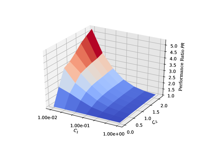
Figure 2: Performance ratio $PR_{\text{LogReg}}$ of synthetic data by $C_{1}$ and $C_{2}$ under Weighted performance metric. The largest performance ratio is for low-skew conditional probabilities (close to uniform) and a high-skew weighted metric.

Table 2: UCI Datasets used in Experiments

Dataset	Instances	Features	Labels	Classes
Car	1727	5	2	4
Nursery	12960	7	2	3
CMC	1473	8	2	4
Phish	1353	7	3	3
Student	649	30	3	5

Table 3: Reports of $\text{PR}_{\text{LogReg}}$ (performance ratio of C-LogReg and LogReg) and $\text{PR}_{\text{DT}}$ (performance ratio of consistent Decision Tree classifier C-DT and Decision Tree classifier DT) by micro- and macro-averaging under Ordinal, Micro-F1 and Weighted${}_{\bf{\frac{1}{2}}}$ performance metrics. Datasets come from UCI Machine Learning Repository and all results average over 100 iterations with 80%-20% train-test split. Consistent algorithms always have better performance.

Dataset	Car	Nursery	CMC	Phish	Student	Car	Nursery	CMC	Phish	Student
	Ordinal metric by Micro-averaging					Ordinal metric by Macro-averaging
$\text{PR}_{\text{LogReg}}$	1.1530	1.0885	1.0181	1.0006	1.0121	1.1485	1.0903	1.0210	1.0005	1.0103
$\text{PR}_{\text{DT}}$	1.1266	1.0687	1.0214	1.0112	1.0124	1.1272	1.0712	1.0212	1.0112	1.0139
	Micro-F1 metric by Micro-averaging					Micro-F1 metric by Macro-averaging
$\text{PR}_{\text{LogReg}}$	1.1972	1.0258	1.0006	1.0001	1.1205	1.2091	1.0391	1.0022	1.0090	1.4144
$\text{PR}_{\text{DT}}$	1.1261	1.0625	1.0006	1.0002	1.1915	1.1190	1.0899	1.0032	1.0146	1.8712
	Weighted${}_{\bf{\frac{1}{2}}}$ metric by Micro-averaging					Weighted${}_{\bf{\frac{1}{2}}}$ metric by Macro-averaging
$\text{PR}_{\text{LogReg}}$	2.4311	1.6060	1.6144	1.3942	1.1211	2.4177	1.6105	1.6327	1.4055	1.1890
$\text{PR}_{\text{DT}}$	3.1338	1.4815	1.6699	1.1235	1.1112	3.1472	1.5057	1.7237	1.2328	1.1012

Table 4: Comparison of performance on Ordinal metric for OrdRec classifier and consistent OrdRec classifier on dataset MovieLens 100k by Micro-averaging and Macro-averaging.

Average	OrdRec	C-OrdRec
Micro	0.8603$\pm$0.0010	0.8640$\pm$0.0009
Macro	0.8577$\pm$0.0032	0.8643$\pm$0.0022

Figure 2 demonstrates the influence of $\mathbf{\bm{C}}_{1}$ and $\mathbf{\bm{C}}_{2}$ on $\text{PR}_{\text{LogReg}}$. For each pair of $\mathbf{\bm{C}}_{1}$ and $\mathbf{\bm{C}}_{2}$, $\text{PR}_{\text{LogReg}}$ is averaged over $30$ iterations with random 80%-20% train-test splits. We observe that the consistent classifier works much better than multi-class logistic regression algorithm with smaller $\mathbf{\bm{C}}_{1}$ and larger $\mathbf{\bm{C}}_{2}$ - we can see that in the dark red region, $\text{PR}_{\text{LogReg}}$ is over 3, which means the performance of C-LogReg is more than three times better than LogReg. To understand the trend of $\text{PR}_{\text{LogReg}}$ through $\mathbf{\bm{C}}_{1}$ and $\mathbf{\bm{C}}_{2}$, notice when the two classifier make different decisions, we have $\sum_{n=1}^{N}\left\llbracket\operatorname*{argmin}_{i\in K}\mathbf{\bm{L}}^{0-1}_{j}\mathbf{\bm{\eta}}_{i}\neq\operatorname*{argmin}_{j\in K}\mathbf{\bm{L}}^{\text{Weighted}}_{j}\mathbf{\bm{\eta}}_{j}\right\rrbracket$, so the classifiers differ when $\sum_{n=1}^{N}\left\llbracket\operatorname*{argmax}_{i\in K}\mathbf{\bm{\eta}}_{i}\neq\operatorname*{argmax}_{j\in K}\mathbf{\bm{A}}_{j}\mathbf{\bm{\eta}}_{j}\right\rrbracket$.

Therefore, the larger the value of $C_{1}$, the more peaked the class probability $\mathbf{\bm{\eta}}_{k}$ for each class $k$, then the effect of $\mathbf{\bm{\eta}}$ becomes more dominant in classification, which results in a smaller difference between two predictions. On the other hand, the larger the value of $C_{2}$, the more skewed $\mathbf{\bm{A}}$ becomes as compared to $\mathbf{\bm{I}}$, resulting in larger difference between two predictions. Furthermore, when $C_{2}=0$, $\mathbf{\bm{A}}$ is exactly $\mathbf{\bm{I}}$, so we have $PR_{\text{LogReg}}=1$ since C-LogReg and LogReg both optimize 0-1 accuracy. The benefit of post-processing must be compared to the additional computational costs. This experiment provides some guidance on this trade-off.

5.2 Benchmark Data: UCI Datasets

We use real-world datasets from UCI repository [16] to evaluate algorithm performances under Ordinal, Micro-F1 and Weighted${}_{\frac{1}{2}}$ metrics by micro-averaging and macro-averaging, as shown in Table 1. Table 2 presents the information about number of instances, features, labels and classes in each of five benchmark datasets we used.

The algorithms evaluated are: (1) multi-output logistic regression classifier for each label (LogReg), (2) Random Forest with max depth as 3 (RF), (3) Decision Tree with max depth as 3 (DT), (4) consistent logistic regression (C-LogReg), (5) consistent Decision Tree (C-DT). (1) and (4) are linear and the rest are non-linear classifiers. The hyper-parameters are chosen using double-loop cross-validation. For simplicity, we only report the performance ratios of $\text{PR}_{\text{LogReg}}$ (performances of C-LogReg over LogReg) and $\text{PR}_{\text{DT}}$ (performances of C-DT over DT) here. See full original performances, variances and more comparisons of algorithms in the Appendix.

Table 2 presents the information about number of instances, features, labels and classes in each of five benchmark datasets. The attributes of each dataset are split into two sets: features and labels. The label assignments are: (1) attributes 1-2 in Car Evaluation (Car), (2) attributes 7-8 in Nursery (Nursery), (3) attributes 7-8 in Contraceptive Method Choice (CMC), (4) attributes 1-3 in Website Phishing (Phish), (5) attributes 26-28 in wiki4HE (wiki4HE). The rest of the attributes are features.

The performance results, averaged over 100 times with random 80%-20% train-test splits, are presented in Table 3. We notice that $\text{PR}_{\text{LogReg}}$ and $\text{PR}_{\text{DT}}$ keep greater than 1, which means that the consistent algorithms always have better performance under same $\widehat{\mathbf{\bm{\eta}}}$: $\Psi(\mathbf{\bm{h}}^{\text{C-LogReg}})>\Psi(\mathbf{\bm{h}}^{\text{LogReg}})$ and $\Psi(\mathbf{\bm{h}}^{\text{C-DT}})>\Psi(\mathbf{\bm{h}}^{DT})$. $\text{PR}_{\text{LogReg}}$ and $\text{PR}_{\text{DT}}$ are enlarged specifically under Weighted${}_{\frac{1}{2}}$ metric.

5.3 Benchmark Data: MovieLens

For the third experiment, we apply multi-output classification to real world rating prediction. We use MovieLens 100K Dataset [6] which contains 100,000 tuples of user, movie and the rating of the user on the movie. We convert the dataset to a standard multi-output classification problem by representing the rating matrix as $Y\in[1,2,..K]^{N\times M}$, where $K$ is the number of rating choices $5$ (star $1$ to star $5$), $N$ is the number of users $943$ and $M$ is number of movies $1,682$ for this dataset. $Y^{(n)}_{m}$ corresponds to the rating of $n-th$ user (sample) $X^{(n)}$ on $m$-th movie (label). We plug in the class probabilities $\mathbf{\bm{\eta}}_{k}^{m}(X^{(n)})=\mathbb{P}(Y^{m}=k|X^{(n)})$ for sample $X^{(n)}$, label $m$ and class $k$. The distribution $\mathbf{\bm{\eta}}$ is derived using the Ordinal regression model OrdRec [11], already shown to perform well for ordinal regression-based prediction.

Once the probabilities are estimated, OrdRec predicts the most likely rating class for each user movie pair.

Since each user only rates a subset of movies, the label space is sparse. We assume that the missing labels are missing at random. Micro-averaging in this setting is equivalent to $\hat{C}_{i,j}(\mathbf{\bm{h}})=\frac{1}{|\Omega|}\sum_{(m,n)\in\Omega}^{M}\hat{C}_{m,i,j}^{(n)}(\mathbf{\bm{h}})$, where $\Omega=\left\{(m,n)\mid\text{$y_{m}^{(n)}$ is observed}\right\}$ is the set of observed entries. In Table 4, we report the micro-averaged and macro-averaged under Ordinal metric on MovieLens dataset of OrdRec and Consistent-OrdRec classifier (C-OrdRec). The results are averaged over 30 times with 50%-50% train-test split. We observe that under all averages, the C-OrdRec classifier results in better performance than OrdRec.

6 Conclusion

We outline necessary and sufficient conditions for Bayes optimal multioutput classification using weighted classifiers – which recovers binary, multiclass and multilabel classification as special cases. We further consider multi-output classification under generalized performance metrics with micro- and macro-averaging, and propose a provably consistent bisection-search classifier for fractional-linear metrics. In a variety of experiments, we find that the proposed estimator can significantly improve performance in practice.

Appendix 0.A Proofs of Weighted Classifier Representation

In this section, we provide the proofs for the theoretical results in the main paper. For ease of navigation, we summarize the notation used in the sequel in Table 5.

Table 5: Notation used in paper

Symbol	Description
$N$	number of instances
$M$	number of outputs
$K$	number of classes
$\mathbf{\bm{C}}\in[0,1]^{K\times M\times M}$	confusion tensor
$\mathcal{U}=\Psi(\mathbf{\bm{C}})$	utility of a classifier
$\Delta_{q}$	$\left\{\mathbf{p}\in[0,1]^{q}:\sum_{i=1}^{q}p_{i}=1\right\}$
$\mathcal{H}_{r}$	set of randomized classifiers $\{\mathbf{h}:\mathcal{X}\to\Delta_{K}^{M}\}$
$\mathbf{\bm{h}}$	multi-output classifier in $\mathcal{H}_{d}$ or $\mathcal{H}_{r}$
$\mathbf{\bm{h}}^{*}_{\Psi}\in\operatorname*{argmax}_{\mathbf{\bm{h}}}\;\mathcal{U}(\mathbf{\bm{h}}).$	Bayes optimal classifier with respect to performance metric $\Psi$.
$\left\llbracket\cdot\right\rrbracket$	indicator function
$\left[q\right]$	$\left\{1,2,\cdots,q\right\}$ for all $q\in\mathbb{Z}_{+}$
$\left\langle\mathbf{\bm{A}},\mathbf{\bm{B}}\right\rangle$	$\sum_{i_{1},\cdots,i_{M}}A_{i_{1},\cdots,i_{M}}B_{i_{1},\cdots,i_{M}}$
$\mathbb{\eta}^{m}_{k}(x)=P(Y_{m}=k|X=x)$	conditional probability for $m$th output and class $k$.
$\mathcal{C}=\left\{\mathbf{\bm{C}}(\mathbf{\bm{h}})\mid\mathbf{\bm{h}}\in\mathcal{H}_{r}\right\}$	set of feasible confusion tensors.
$e_{i}$	$i$th standard basis whose $i$th dimension is 1 and 0 otherwise $e_{i}=(0,\cdots,1,\cdots,0)$
$\bm{1}_{M}\in\mathbb{R}^{M}$	all one vector of dimension $M$
$\bm{v}\otimes\bm{w}$	outer product, $(\bm{v}\otimes\bm{w})_{ij}=v_{i}w_{j}$

0.A.1 Proof of Lemma 1

Observe that $\mathcal{H}$ is equivalent to the space of vector $L_{\infty}$ functions which is a compact function space.

• Compact: Compactness of $\mathcal{C}$ follows from compactness of $\mathcal{H}$, since the mapping $C:\mathcal{H}\mapsto[0,1]^{M\times K\times K}$ is linear and bounded.

• Convex: Suppose $\mathbf{C}_{1}=\mathbf{\bm{C}}(h_{1}),\mathbf{C}_{2}=\mathbf{\bm{C}}(h_{2})\in\mathcal{C}$. For any $\mathbf{C}_{0}=\alpha\mathbf{C}_{1}+(1-\alpha)\mathbf{C}_{2}$, by linearity of expectation, we have that $\mathbf{C}_{0}=C(h_{0})$ where $h_{0}=\alpha h_{1}+(1-\alpha)h_{2}$ .

0.A.2 Proof of Lemma 2 and Lemma 3

The proof of Lemma 2 is primarily geometric, and utilizes the following lemma characterizing supporting hyperplanes of convex sets.

Lemma 5 (Supporting Hyperplane [23])

Let $\mathcal{S}$ be a compact convex set, then for every $\mathbf{s}\in\partial\mathcal{S}$ there exists a supporting hyperplane which intersects with $\mathcal{S}$ at $\mathbf{s}$.

As a result, given $\mathbf{a}$ as the normal of hyperplane associated with a point $\mathbf{s}*\in\partial\mathcal{S}$, if follows that:

$$\mathbf{s}*\in\underset{s\in\mathcal{S}}{\text{argmax}}\left\langle\mathbf{a},\mathbf{s}\right\rangle$$

Thus, $\mathcal{S}$ has a dual representation, as the intersection of all the half-spaces associated with its supporting hyperplanes.

Proof (Proof of Lemma 2)

By the compactness of $\mathcal{C}$, there exists a $\mathbf{\bm{C}}^{*}$ such that $\mathbf{\bm{C}}^{*}=\arg\max_{\mathbf{\bm{C}}\in\mathcal{C}}\Psi(\mathbf{\bm{C}})$. Hence there exists $\mathbf{h}^{*}\in\mathcal{H}_{r}$ such that $\mathbf{\bm{C}}^{*}=\mathbf{\bm{C}}(\mathbf{h}^{*})$. Equivalently, $\mathbf{h}^{*}=\arg\max_{\mathbf{h}\in\mathcal{H}_{r}}\mathcal{U}(\mathbf{h})$. Let $\mathbf{C}^{*}\in\partial\mathcal{C}$, then this implies that $\exists\mathbf{L}$ such that:

$$\mathbf{C}^{*}=\mathbf{C}(h^{*})\in\operatorname*{argmax}_{\mathbf{C}\in\mathcal{C}}\left\langle\mathbf{L},\mathbf{\bm{C}}\right\rangle,$$

where $h^{*}\in\operatorname*{argmax}_{h\in\mathcal{H}}\left\langle\mathbf{A}^{*},\mathbf{\bm{C}}(h)\right\rangle$. When $\mathbb{P}$ satisfies Assumption 1, this is equivalent to a linear utility metric. For this case, [17] have shown that the max classifier is Bayes optimal almost everywhere.

Proof (Proof of Lemma 3)

$\operatorname*{argmax}_{\mathbf{C}\in\mathcal{C}}\left\langle\mathbf{L},\mathbf{\bm{C}}\right\rangle$ is the optimization of a linear function over a compact convex set $\mathcal{C}$, thus the maximum $\mathbf{\bm{C}}^{*}$ is necessarily achieved at the boundary $\mathbf{\bm{C}}^{*}\in\partial\mathcal{C}$.

0.A.3 Proof of Lemma 4

When $\Phi$ is a monotonic function of $\mathbf{\bm{C}}$, then $\mathbf{\bm{C}}^{*}$ necessarily lies on $\partial\mathcal{C}$. By Lemma 3, we know that the Bayes optimal follows the weighted form. By KKT conditions [2], when $\mathbf{\bm{C}}^{*}$ is optimal, the supporting hyperplane must equal the negative gradient of the metric at $\mathbf{\bm{C}}^{*}$. The remainder follows from the scale and shift invariance of the loss matrix.

0.A.4 Proof of Theorem 3.1

Let $\mathbf{\bm{L}}$ be as defined in Lemma 2. By definition in Eq. (1), we have

$$\max_{\mathbf{\bm{C}}}\left\langle\mathbf{\bm{L}},\mathbf{\bm{C}}\right\rangle= \max_{\mathbf{\bm{C}}}\sum_{m,k,\ell}\mathbf{\bm{L}}_{m,k,\ell}\mathbf{\bm{C}}_{m,k,\ell}$$

$$= \max_{\mathbf{h}}\sum_{m,k,\ell}\mathbf{\bm{L}}_{m,k,\ell}\int_{x}\mathbf{h}_{k}^{m}(x)\mathbb{\eta}^{m}_{\ell}(x)d\mathbb{P}(x)$$

Note the above maximization is decomposable with respect to $x$ given $\mathbb{\eta}(x)$. For any given $x$, to maximize $\sum_{m,k,\ell}\mathbf{\bm{L}}_{m,k,\ell}\mathbf{h}_{k}^{m}(x)\mathbb{\eta}^{m}_{\ell}(x)$ subject to the constraint that $\sum_{k}\mathbf{h}_{k}^{m}(x)=1,\mathbf{h}_{k}^{m}\geq 0$ is equivalent to finding the largest index $k^{*}$ such that $k^{*}=\arg\min\left\langle\mathbf{\bm{L}}_{m,k,\cdot},\mathbf{\bm{\eta}}^{m}\right\rangle$, and set $h_{k^{*}}^{m}=1$ and 0 otherwise. This completes the proof.

Appendix 0.B Proofs for averaging metrics

Proof (Proof of Proposition 1)

By definition,

$$\Psi_{\text{micro}}(\mathbf{\bm{\widehat{C}}})=\psi\left(\widehat{\mathbf{\bm{C}}}\mathchoice{\mathbin{\vbox{\hbox{\scalebox{1.0}{$\displaystyle\bullet$}}}}}{\mathbin{\vbox{\hbox{\scalebox{1.0}{$\textstyle\bullet$}}}}}{\mathbin{\vbox{\hbox{\scalebox{1.0}{$\scriptstyle\bullet$}}}}}{\mathbin{\vbox{\hbox{\scalebox{1.0}{$\scriptscriptstyle\bullet$}}}}}_{1}\frac{1}{M}\bm{1}_{M}\right)$$

Taking derivative with respect to $\mathbf{\bm{C}}_{m,k,\ell}$, by the chain rule we have

$$\nabla_{m,k,\ell}\Psi(\mathbf{\bm{C}})= \nabla_{k,\ell}\psi\left(\frac{1}{M}\sum_{m=1}^{M}\mathbf{\bm{C}}_{m,\cdot,\cdot}\right)e_{k}\otimes e_{\ell}\otimes\frac{1}{M}\bm{1}_{M},$$

where $e_{k}$ is the $k{{}^{th}}$ standard normal vector. Hence,

$$\nabla\Psi(\mathbf{\bm{C}})= \nabla\psi\left(\frac{1}{M}\sum_{m=1}^{M}\mathbf{\bm{C}}_{m,\cdot,\cdot}\right)\otimes\frac{1}{M}\bm{1}_{M}$$

By Lemma 4, the supporting hyper-plane is $-\nabla\psi\left(\frac{1}{M}\sum_{m=1}^{M}\mathbf{\bm{C}}^{*}_{m,\cdot,\cdot}\right)\otimes\frac{1}{M}\bm{1}_{M}$. By its formulation, we know each slice along the 3rd dimension is the same matrix $-\nabla\psi\left(\frac{1}{M}\sum_{m=1}^{M}\mathbf{\bm{C}}^{*}_{m,\cdot,\cdot}\right)$, the claim is proved.

Appendix 0.C Proof of Proposition 2

Proposition 3 (Decomposability of macro-averaged Bayes Optimal)

The macro averaged utility decomposes as $\mathcal{U}_{\text{macro}}(\mathbf{\bm{h}})=\sum_{m\in[M]}\mathcal{U}_{m}(h_{m})$, and the Bayes optimal macro-averaged classifier decomposes as: $h_{m}^{*}(x)=\underset{h_{m}}{\operatorname*{argmax}}\;\mathcal{U}_{m}(h_{m})$.

Proof

The proof follows by definition. The confusion matrix at the population level, instead of calculating from the samples, is replaced by the expectation:

$$(\mathbf{\bm{C}}_{m})_{i,j}(\mathbf{\bm{h}}) =\mathbb{E}\left[(\widehat{C}_{m})_{i,j}(\mathbf{\bm{h}})\right]$$

$$=\frac{1}{N}\sum_{n=1}^{N}\mathbb{E}_{n}\left[\widehat{\mathbf{\bm{C}}}_{m,i,j}^{(n)}(h_{m})\right]$$

$$=\Pr\left(Y_{m}=i,h_{m}(X)=j\right)$$

and the utility at population level is given by

$$\mathcal{U}_{\text{macro}}(\mathbf{\bm{h}})=\frac{1}{M}\sum_{m=1}^{M}\Psi\left(\mathbf{\bm{C}}_{m}(h_{m})\right)$$

Specifically, the utility of loss-based performance metric is given by

$$\mathcal{U}_{\text{macro}}(\mathbf{\bm{h}}) =\frac{1}{M}\sum_{m=1}^{M}\Psi^{\mathbf{\bm{L}}^{m}}(\mathbf{\bm{C}}_{m}(h_{m}))$$

$$=\frac{1}{M}\sum_{m=1}^{M}\left[1-\left\langle\mathbf{\bm{L}}^{m},\mathbf{\bm{C}}_{m}(h_{m})\right\rangle\right]$$

$$=1-\frac{1}{M}\sum_{m=1}^{M}\left[\left\langle\mathbf{\bm{L}}^{m},\mathbf{\bm{C}}_{m}(h_{m})\right\rangle\right]$$

Appendix 0.D Proof of Theorem 0.E.1

Theorem 0.D.1 ($\Psi$-regret of bisection based algorithm)

($\Psi$-regret of bisection based algorithm). Let $\psi:\left[0,1\right]^{K\times K}\to\mathbb{R}_{+}$ be $\psi(\mathbf{\bm{C}})=\frac{\left\langle\mathbf{\bm{A}},\mathbf{\bm{C}}\right\rangle}{\left\langle\mathbf{\bm{B}},\mathbf{\bm{C}}\right\rangle}$, where $\mathbf{\bm{A}}$, $\mathbf{\bm{B}}\in\mathbb{R}^{K\times K}_{+}$, $\sup_{(\mathbf{\bm{C}})\in\mathcal{C}_{\mathbb{P}}}\psi{(\mathbf{\bm{C}})}\leq 1$, and $\min_{\mathbf{\bm{C}}\in\mathcal{C}_{\mathbb{P}}}\left\langle\mathbf{\bm{B}},\mathbf{\bm{C}}\right\rangle\geq b$, for some $b>0$. Let $\mathcal{S}=(\mathcal{S}_{1},\mathcal{S}_{2})\in{(\mathcal{X}\times\mathcal{Y})}^{N}$ be a training set drawn i.i.d from a distribution $\mathbb{P}$, where $\mathcal{Y}=\left[K\right]^{M}$. Let $\widehat{\mathbf{\bm{\eta}}}:\mathcal{X}\to[\Delta_{K}]^{M}$ be the model learned from $\mathcal{S}_{1}$ in Algorithm 1 and $\mathbf{\bm{h}}^{BS}:\mathcal{X}\to\mathcal{Y}$ be the classifier obtained over $\kappa N$ iterations. Then for any $\delta\in(0,1]$, with probability at least $1-\delta$ (over draw of $\mathcal{S}$ from $\mathbb{P}^{N}$), we have

$$\mathcal{U}^{*}_{\mathbb{P}} -\mathcal{U}_{\mathbb{P}}{[\mathbf{\bm{h}}^{BS}]}\leq\frac{2\tau}{m}\sum_{m}\mathbb{E}_{X}\left[\left\lVert\widehat{\mathbf{\bm{\eta}}}^{m}(X)-{\mathbf{\bm{\eta}}^{m}(X)}\right\rVert_{1}\right]+$$

$$2\sqrt{2}C_{\tau}\sqrt{\frac{K^{2}\log(K)\log(MN)+\log(K^{2}/\delta)}{MN}}+2^{-\kappa MN}$$

where $\tau=\frac{1}{b}(||A||_{1}+||B||_{1})$ and $C>0$ is a distribution-independent constant.

Proof

We prove by exploring the equivalent multi-class classification under multi-output classification paradigm. Let $Z=[X,O]$ denotes a new instance space $\mathcal{Z}$ that adds a feature $m$ to $\mathcal{X}$ space, with $\Pr\left(Z\right)=\Pr\left(X\right)\Pr\left(O\right)$ and uniform label distribution that $\Pr\left(O=m\right)=\frac{1}{m}$. Then we construct a multi-class classification with $NM$ instances where $\mathcal{Z}\to\Delta_{K}$.

According to definition, we have new label space, classifier $f(z)$, conditional distribution $\gamma(z)$ and marginal distribution $\Pr\left(Z\right)$ as

$$Y_{z}=Y_{m}(x)\in[K]$$

$$f(z)=h_{m}(x)\in[K]$$

$$\mathbf{\bm{\gamma}}(z)=\mathbf{\bm{\eta}}^{m}(x)$$

$$\Pr\left(z\right)=\frac{1}{m}\Pr\left(x\right)$$

The confusion matrix $D(f)$ is

$$D_{i,j}(f) =\mathbb{E}_{z}\mathbb{E}_{y,z}(\left\llbracket y=i,f(z)=j\right\rrbracket)$$

$$=\frac{1}{m}\sum_{m=1}^{M}\mathbb{E}_{x}\mathbb{E}_{y,x}(\left\llbracket y_{m}=i,h_{m}(x)=j\right\rrbracket)$$

$$=\frac{1}{m}C_{i,j}(h_{m})$$

And the optimal classifier $f^{*}(z)$ is

$$f^{*}(z) =\operatorname*{argmin}_{k\in[K]}\mathbf{\bm{\gamma}}(z)^{T}L_{k}=\operatorname*{argmin}_{k\in[K]}(\mathbf{\bm{\eta}}^{m})^{T}{(x)}L_{k}$$

Then, the multi-class classification $\mathcal{Z}\to\Delta_{K}$ is equivalent to the original multi-output classification ${(\mathcal{X}\times\left[K\right]^{M})}^{N}\to[\Delta_{K}]^{M}$. By Theorem 17 in  [17], we have

$$\mathcal{U}^{*}_{\mathbb{P}}-\mathcal{U}_{\mathbb{P}}{[\mathbf{\bm{h}}^{BS}]}\leq 2\tau\mathbb{E}_{Z}\left[\left\lVert\widehat{\mathbf{\bm{\gamma}}}(Z)-{\mathbf{\bm{\gamma}}(Z)}\right\rVert_{1}\right]$$

$$+2\sqrt{2}C_{\tau}\sqrt{\frac{K^{2}\log(K)\log(MN)+\log(K^{2}/\delta)}{MN}}+2^{-\kappa MN},$$

Also note that

$$\mathbb{E}_{Z}\left[f(Z)\right] =\mathbb{E}_{m}\mathbb{E}_{X}\left[f([X,m])\right]$$

$$=\frac{1}{m}\sum_{m}\mathbb{E}_{x}\left[\left\lVert\widehat{\mathbf{\bm{\eta}}}^{m}(X)-\mathbf{\bm{\eta}}^{m}(X)\right\rVert_{1}\right]$$

Then finally, we have

$$\mathcal{U}^{*}_{\mathbb{P}}-\mathcal{U}_{\mathbb{P}}{[\mathbf{\bm{h}}^{BS}]}\leq\frac{2\tau}{m}\sum_{m}\mathbb{E}_{X}\left[\left\lVert\widehat{\mathbf{\bm{\eta}}}^{m}(X)-{\mathbf{\bm{\eta}}^{m}(X)}\right\rVert_{1}\right]$$

$$+2\sqrt{2}C_{\tau}\sqrt{\frac{K^{2}\log(K)\log(MN)+\log(K^{2}/\delta)}{MN}}+2^{-\kappa MN},$$

Appendix 0.E Bisection Method - Algorithm

Algorithm 1 Bisection Method (for micro averaging of multi-class fractional linear metrics)

Input:	$\mathcal{S}=\left\{x^{(n)},\mathbf{\bm{y}}^{(n)}\right\}_{n=1}^{N}\in(\mathcal{X}\times\left[K\right]^{M})^{N}$
	$\Psi(\mathbf{\bm{C}})=\frac{\left\langle\mathbf{\bm{A}},\mathbf{\bm{C}}\right\rangle}{\left\langle\mathbf{\bm{B}},\mathbf{\bm{C}}\right\rangle}$ where $\mathbf{\bm{A}},\mathbf{\bm{B}}\in\mathbb{R}^{K\times K}$.

Parameter: $\kappa\in\mathbb{N}$

1:  Split $\mathcal{S}$ into $\mathcal{S}_{1}$ and $\mathcal{S}_{2}$ with size $\left\lceil\frac{N}{2}\right\rceil$ and $\left\lfloor\frac{N}{2}\right\rfloor$; estimate $\widehat{\mathbf{\bm{\eta}}}=\left\{\widehat{\mathbf{\bm{\eta}}}^{m}\right\}_{m=1}^{M}$ using $\mathcal{S}_{1}$

2:  Initialize $\mathbf{\bm{h}}^{0}:\mathcal{X}\to\left[K\right]^{M}$, $\alpha=0$, $\beta=1$

3:  for $t=1$ to $\kappa N$ do

4:     $\gamma^{t}=(\alpha^{t-1}+\beta^{t-1})/2$

5:     $\widehat{\mathbf{\bm{L}}}^{t}=\gamma^{t}\mathbf{\bm{B}}-\mathbf{\bm{A}}$, scaled and shifted to $\left[0,1\right]^{K\times K}$.

6:     Define $\mathbf{\bm{\widehat{g}}}^{t}=\left\{\widehat{g}^{t}_{m}\right\}_{m=1}^{M}$ where ${\widehat{g}^{t}_{m}(x)}\in{\operatorname*{argmin}_{k\in\left[K\right]}(\mathbf{\bm{\widehat{L}}}_{k}^{t})^{\intercal}\mathbf{\bm{\widehat{\eta}}}^{m}(x)}$

7:     if $\widehat{\mathcal{U}}^{\mathcal{S}_{2}}_{\text{micro}}(\mathbf{\widehat{g}}^{t})\geq\gamma^{t}$ then

8:        $\alpha^{t}=\gamma^{t}$, $\beta^{t}=\beta^{t-1}$, $\mathbf{\bm{h}}^{t}=\mathbf{\bm{\widehat{g}}}^{t}$

9:     else

10:        $\alpha^{t}=\alpha^{t-1}$, $\beta^{t}=\gamma^{t}$, $\mathbf{\bm{h}}^{t}=\mathbf{\bm{h}}^{t-1}$

11:     end if

12:  end for

Output: $\mathbf{\bm{h}}^{(\kappa N)}$

0.E.1 Consistency of Bisection Algorithm

Consistency is a desirable property for a classifier, as it suggests that the procedure has good large sample statistical properties.

Theorem 0.E.1

($\Psi$-regret of bisection based algorithm). Let $\psi:\left[0,1\right]^{K\times K}\to\mathbb{R}_{+}$ be $\psi(\mathbf{\bm{C}})=\frac{\left\langle\mathbf{\bm{A}},\mathbf{\bm{C}}\right\rangle}{\left\langle\mathbf{\bm{B}},\mathbf{\bm{C}}\right\rangle}$, where $\mathbf{\bm{A}}$, $\mathbf{\bm{B}}\in\mathbb{R}^{K\times K}_{+}$, $\sup_{(\mathbf{\bm{C}})\in\mathcal{C}_{\mathbb{P}}}\psi{(\mathbf{\bm{C}})}\leq 1$, and $\min_{\mathbf{\bm{C}}\in\mathcal{C}_{\mathbb{P}}}\left\langle\mathbf{\bm{B}},\mathbf{\bm{C}}\right\rangle\geq b$, for some $b>0$. Let $\mathcal{S}=(\mathcal{S}_{1},\mathcal{S}_{2})\in{(\mathcal{X}\times\mathcal{Y})}^{N}$ be a training set drawn i.i.d from a distribution $\mathbb{P}$, where $\mathcal{Y}=\left[K\right]^{M}$. Let $\widehat{\mathbf{\bm{\eta}}}:\mathcal{X}\to[\Delta_{K}]^{M}$ be the model learned from $\mathcal{S}_{1}$ in Algorithm 1 and $\mathbf{\bm{h}}^{BS}:\mathcal{X}\to\mathcal{Y}$ be the classifier obtained over $\kappa N$ iterations. Then for any $\delta\in(0,1]$, with probability at least $1-\delta$ (over draw of $\mathcal{S}$ from $\mathbb{P}^{N}$), we have $\mathcal{U}^{*}_{\mathbb{P}}-\mathcal{U}_{\mathbb{P}}{[\mathbf{\bm{h}}^{BS}]}\leq\frac{2\tau}{m}\sum_{m}\mathbb{E}_{X}\left[\left\lVert\widehat{\mathbf{\bm{\eta}}}^{m}(X)-{\mathbf{\bm{\eta}}^{m}(X)}\right\rVert_{1}\right]+2\sqrt{2}C_{\tau}\sqrt{\frac{K^{2}\log(K)\log(MN)+\log(K^{2}/\delta)}{MN}}+2^{-\kappa MN},$ where $\tau=\frac{1}{b}(||A||_{1}+||B||_{1})$ and $C>0$ is a distribution-independent constant.

Appendix 0.F Additional Discussion of Averaged Multioutput Metrics

Table 6: Confusions and performance metrics for three averagings

Averaging	Confusion	Performance Metric
Micro-averaging	$\widehat{C}_{i,j}(\mathbf{\bm{h}})=\frac{1}{MN}\sum_{m=1}^{M}\sum_{n=1}^{N}\widehat{C}_{m,i,j}^{(n)}(h_{m})$	$\Psi_{\text{micro}}(\mathcal{A}(\mathbf{\bm{h}}))=\psi\left(\mathbf{\bm{\widehat{C}}}(\mathbf{\bm{h}})\right)$
Instance-averaging	$(\widehat{C}_{n})_{i,j}(\mathbf{\bm{h}})=\frac{1}{M}\sum_{m=1}^{M}\widehat{C}_{m,i,j}^{(n)}(h_{m})$	$\Psi_{\text{instance}}(\mathcal{A}(\mathbf{\bm{h}}))=\frac{1}{N}\sum_{n=1}^{N}\psi\left(\mathbf{\bm{\widehat{C}}}_{n}(\mathbf{\bm{h}})\right)$
Macro-averaging	$(\widehat{C}_{m})_{i,j}(\mathbf{\bm{h}})=\frac{1}{N}\sum_{n=1}^{N}\widehat{C}_{m,i,j}^{(n)}(h_{m})$	$\Psi_{\text{macro}}(\mathcal{A}(\mathbf{\bm{h}}))=\frac{1}{M}\sum_{m=1}^{M}\psi\left(\mathbf{\bm{\widehat{C}}}_{m}(h_{m})\right)$

The most common technique for constructing multioutput metrics is by averaging multiclass performance metrics, which corresponds to particular settings of $\mathcal{A}(\mathbf{\bm{h}})$. Averaged multiclass metrics are constructed by averaging with respect to outputs (instance-averaging), with respect to examples separately for each output (macro-averaging), or with respect to both outputs and examples (micro-averaging). The confusions and performance metrics for micro-, macro- and instance-averaging are straightforward to derive from their definitions, and are as shown in Table 6.

Now we turn our attention to characterizing the Bayes optimal classifiers for averaged multioutput metrics. Our first observation is that micro-averaging and instance-averaging, while seemingly quite different in terms of samples, are in fact equivalent as population metrics. Note that our definitions of population metrics directly follow from the multilabel classification definitions established by  Koyejo et al. [13]

Proposition 4 (Micro- and Instance-averaging are equivalent at population level)

Given $\Psi$, for any $\mathbf{\bm{h}}$, $\mathcal{U}_{\text{instance}}(\mathbf{\bm{h}})=\mathcal{U}_{\text{micro}}(\mathbf{\bm{h}})=\Psi\left(\frac{1}{M}\sum_{m=1}^{M}\mathbf{\bm{C}}(h_{m})\right),$ and consequently, $\mathbf{\bm{h}}^{*}_{\Psi_{\text{instance}}}=\mathbf{\bm{h}}^{*}_{\Psi_{\text{micro}}}$

Proof

For micro-averaging, at the population level, instead of calculating the confusion from the samples, we replace it by the expectation of the confusions:

$$C_{i,j}(\mathbf{\bm{h}}) =\mathbb{E}\left[\widehat{C}_{i,j}(\mathbf{\bm{h}})\right]$$

$$=\frac{1}{M}\sum_{m=1}^{M}\mathbb{E}_{n}\left[\widehat{C}_{m,i,j}^{(n)}(h_{m})\right]$$

$$=\frac{1}{M}\sum_{m=1}^{M}\Pr\left(Y_{m}=i,h_{m}(X)=j\right)$$

and the performance at population level is given by

$$\mathcal{U}_{\text{micro}}(\mathbf{\bm{h}})=\psi\left(\mathbf{\bm{C}}(\mathbf{\bm{h}})\right)$$

Similarly, for instance-averaging, we replace the sample confusion matrix by its expectation:

$$(C_{n})_{i,j}(\mathbf{\bm{h}}) =\mathbb{E}\left[(\widehat{C}_{n})_{i,j}(\mathbf{\bm{h}})\right]$$

$$=\frac{1}{M}\sum_{m=1}^{M}\mathbb{E}_{n}\left[\widehat{C}_{m,i,j}^{(n)}(h_{m})\right]$$

$$=\frac{1}{M}\sum_{m=1}^{M}\Pr\left(Y_{m}=i,h_{m}(X)=j\right)$$

Since $(\mathbf{\bm{C}}_{n})(\mathbf{\bm{h}})$ is the same for every $n$, we can write it as $\mathbf{\bm{C}}(\mathbf{\bm{h}})$ instead. The performance at population level is then given by

$$\mathcal{U}_{\text{instance}}(\mathbf{\bm{h}}) =\frac{1}{N}\sum_{n=1}^{N}\psi\left(\mathbf{\bm{C}}(\mathbf{\bm{h}})\right)$$

$$=\psi\left(\mathbf{\bm{C}}(\mathbf{\bm{h}})\right)$$

For loss-based performance metric, define $\mathbf{\bm{C}}_{m}(h_{m})=\mathbb{E}_{n}\left[\mathbf{\bm{\widehat{C}}}_{m}^{(n)}(h_{m})\right]$, the utility of $\Psi^{\mathbf{\bm{L}}}$ is given by

$$\mathcal{U}_{\text{micro}}(\mathbf{\bm{h}})=\mathcal{U}_{\text{instance}}(\mathbf{\bm{h}}) =\psi^{\mathbf{\bm{L}}}(\mathbf{\bm{C}}(\mathbf{\bm{h}}))$$

$$=1-\left\langle\mathbf{\bm{L}},\mathbf{\bm{C}}(\mathbf{\bm{h}})\right\rangle$$

$$=1-\left\langle\mathbf{\bm{L}},\frac{1}{M}\sum_{m=1}^{M}\mathbf{\bm{C}}_{m}(h_{m})\right\rangle$$

$$=1-\frac{1}{M}\sum_{m=1}^{M}\left\langle\mathbf{\bm{L}},\mathbf{\bm{C}}_{m}(h_{m})\right\rangle$$

Therefore, the optimal classifier $\mathbf{\bm{h}}^{*}$ that maximize $\mathcal{U}$ is also the one that minimize $\frac{1}{M}\sum_{m=1}^{M}\left\langle\mathbf{\bm{L}},\mathbf{\bm{C}}_{m}(h_{m})\right\rangle$. This is equivalent to finding the minimum of each of $\left\langle\mathbf{\bm{L}},\mathbf{\bm{C}}_{m}(h_{m})\right\rangle$ independently.

Similar to [17], the optimal classifier $\mathbf{\bm{h}}^{*}:\mathcal{X}\to\left[K\right]^{M}$ satisfies

$$h^{*}_{m}(x)\in\operatorname*{argmin}_{k\in\left[K\right]}\mathbf{\bm{L}}_{k}^{\intercal}\mathbf{\bm{\eta}}^{m}(x)$$

and we call $h^{*}$ the $\Psi^{\mathbf{\bm{L}}}$ optimal classifier.

Appendix 0.G Experiments Details and More Results

We report the full results for micro- and macro-averaging on benchmark datasets in Table 7. The algorithms evaluated are: (1) multi-output logistic regression classifier for each label (LogReg), (2) k-nearest neighbor with k as 5 (KNN), (3) Random Forest with max depth as 3 (RF), (4) Decision Tree with max depth as 3 (DT), (5) consistent logistic regression (C-LogReg), (6) consistent Decision Tree (C-DT). (1) and (5) are linear and the rest are non-linear classifiers. The hyper-parameters are chosen using double-loop cross-validation.

As expected, C-DT or C-LogReg always gives the best performance. The difference between C-DT and C-LogReg comes from their consumption of class probabilities from different base learners.

Table 7: Comparison of performance for multi-output over logistic regression (LogReg), k-nearest neighbors (KNN), Random Forests (RF), Decision Tree (DT), consistent multi-output logistic regression classifier (C-LogReg), consistent Decision Tree classifier (C-DT) by micro- and macro-averaging under Ordinal, Micro-F1 and Weighted${}_{\bf{\frac{1}{2}}}$ performance metrics. Datasets come from UCI Machine Learning Repository and all results average over 100 iterations with 80%-20% train-test split. The last two columns are the proposed post-processing which we found always improved performance.

Dataset LogReg KNN RF DT C-LogReg C-DT Comparison of performance on Ordinal metric for six algorithms on benchmark datasets by Micro-averaging Car 0.6038$\pm$0.0128 0.5799$\pm$0.0126 0.6112$\pm$0.0169 0.6170$\pm$0.0228 0.6962$\pm$0.0075 0.6961$\pm$0.0076 Nursery 0.7047$\pm$0.0090 0.6223$\pm$0.0035 0.7084$\pm$0.0148 0.7173$\pm$0.0132 0.7671$\pm$0.0032 0.7666$\pm$0.0030 CMC 0.7777$\pm$0.0109 0.7443$\pm$0.0100 0.7644$\pm$0.0123 0.7654$\pm$0.0137 0.7918$\pm$0.0098 0.7818$\pm$0.0097 Phish 0.7967$\pm$0.0087 0.7787$\pm$0.0103 0.7888$\pm$0.0157 0.7981$\pm$0.0096 0.8016$\pm$0.0084 0.8070$\pm$0.0089 Student 0.7704$\pm$0.0122 0.7585$\pm$0.0130 0.7778$\pm$0.0119 0.7792$\pm$0.0119 0.7797$\pm$0.0122 0.7889$\pm$0.0122 Comparison of performance on Micro-F1 metric for six algorithms on benchmark datasets by Micro-averaging Car 0.2775$\pm$0.0191 0.1573$\pm$0.0137 0.2784 $\pm$ 0.0231 0.2941$\pm$0.0194 0.3322$\pm$0.0175 0.3312$\pm$0.0187 Nursery 0.4836$\pm$0.0084 0.2896$\pm$0.0067 0.4531$\pm$0.0307 0.4815$\pm$0.0159 0.4961$\pm$0.0074 0.5116$\pm$0.0070 CMC 0.4928$\pm$0.0200 0.4155$\pm$0.0195 0.4870$\pm$0.0176 0.4737$\pm$0.0188 0.4959$\pm$0.0189 0.4767$\pm$0.0199 Phish 0.6931$\pm$0.0175 0.6860$\pm$0.0182 0.6868$\pm$0.0226 0.7029$\pm$0.0168 0.6941$\pm$0.0182 0.7040$\pm$0.0191 Student 0.2291$\pm$0.0232 0.2240$\pm$0.0273 0.2299$\pm$0.0286 0.2413$\pm$0.0276 0.2567$\pm$0.0247 0.2875$\pm$0.0269 Comparison of performance on Weighted${}_{\bf{\frac{1}{2}}}$ metric for six algorithms on benchmark datasets by Micro-averaging Car 0.1023$\pm$0.0124 0.0754$\pm$0.0095 0.0526$\pm$0.0094 0.0792$\pm$0.0245 0.2487$\pm$0.0152 0.2482$\pm$0.0153 Nursery 0.2218$\pm$0.0144 0.2203$\pm$0.0045 0.2361$\pm$0.0172 0.2405$\pm$0.0253 0.3562$\pm$0.0060 0.3563$\pm$0.0060 CMC 0.1206$\pm$0.0098 0.1228$\pm$0.0095 0.1124$\pm$0.0115 0.1151$\pm$0.0109 0.1947$\pm$0.0118 0.1922$\pm$0.0119 Phish 0.2260$\pm$0.0164 0.2270$\pm$0.0169 0.2286$\pm$0.0211 0.2541$\pm$0.0194 0.3151$\pm$0.0210 0.3139$\pm$0.0208 Student 0.3073$\pm$0.0195 0.3048$\pm$0.0164 0.3544$\pm$0.0190 0.3344$\pm$0.0224 0.3721$\pm$0.0209 0.3716$\pm$0.0215 Comparison of performance on Ordinal metric for six algorithms on benchmark datasets by Macro-averaging Car 0.6060$\pm$0.0127 0.5788$\pm$0.0107 0.6131$\pm$0.0176 0.6185$\pm$0.0219 0.6960$\pm$0.0078 0.6972$\pm$0.0085 Nursery 0.7043$\pm$0.0088 0.6230$\pm$0.0036 0.7022$\pm$0.0145 0.7164$\pm$0.0141 0.7679$\pm$0.0028 0.7672$\pm$0.0028 CMC 0.7748$\pm$0.0104 0.7445$\pm$0.0095 0.7643$\pm$0.0119 0.7642$\pm$0.0146 0.7911$\pm$0.0087 0.7804$\pm$0.0083 Phish 0.7977$\pm$0.0095 0.7871$\pm$0.0150 0.7871$\pm$0.0150 0.7983$\pm$0.0094 0.8015$\pm$0.0096 0.8065$\pm$0.0093 Student 0.7698$\pm$0.0119 0.7581$\pm$0.0118 0.7761$\pm$0.0136 0.7778$\pm$0.0132 0.7785$\pm$0.0111 0.7886$\pm$0.0114 Comparison of performance on Micro-F1 metric for six algorithms on benchmark datasets by Macro-averaging Car 0.2759$\pm$0.0163 0.1562$\pm$0.0153 0.2762$\pm$0.0191 0.2939$\pm$0.0184 0.3336$\pm$0.0167 0.3289$\pm$0.0166 Nursery 0.4862$\pm$0.0112 0.2784$\pm$0.0072 0.4510$\pm$0.0333 0.4763$\pm$0.0241 0.5052$\pm$0.0072 0.5190$\pm$0.0074 CMC 0.4898$\pm$0.0210 0.4113$\pm$0.0195 0.4837$\pm$0.0206 0.4722$\pm$0.0211 0.4909$\pm$0.0188 0.4737$\pm$0.0204 Phish 0.6853$\pm$0.0165 0.6767$\pm$0.0162 0.6826$\pm$0.0199 0.6938$\pm$0.0177 0.6915$\pm$0.0182 0.7039$\pm$0.0181 Student 0.1728$\pm$0.0252 0.1887$\pm$0.0267 0.1189$\pm$0.0143 0.1522$\pm$0.0208 0.2444$\pm$0.0218 0.2848$\pm$0.0292 Comparison of performance on Weighted${}_{\bf{\frac{1}{2}}}$ metric for six algorithms on benchmark datasets by Macro-averaging Car 0.1027$\pm$0.0111 0.0736$\pm$0.0097 0.0529$\pm$0.0099 0.0788$\pm$0.0238 0.2483$\pm$0.0121 0.2480$\pm$0.0120 Nursery 0.2213$\pm$0.0137 0.2202$\pm$0.0044 0.2340$\pm$0.0171 0.2367$\pm$0.0255 0.3564$\pm$0.0055 0.3564$\pm$0.0055 CMC 0.1187$\pm$0.0108 0.1216$\pm$0.0116 0.1092$\pm$0.0120 0.1111$\pm$0.0125 0.1938$\pm$0.0130 0.1915$\pm$0.0128 Phish 0.2259$\pm$0.0134 0.2286$\pm$0.0158 0.2312$\pm$0.0207 0.2564$\pm$0.0166 0.3175$\pm$0.0163 0.3161$\pm$0.0158 Student 0.3117$\pm$0.0214 0.3047$\pm$0.0209 0.3540$\pm$0.0231 0.3360$\pm$0.0233 0.3706$\pm$0.0242 0.3700$\pm$0.0261

References

- Borchani et al. [2012] Hanen Borchani, Concha Bielza, Pablo Martí nez Martín, and Pedro Larrañaga. Markov blanket-based approach for learning multi-dimensional Bayesian network classifiers: An application to predict the European Quality of Life-5 Dimensions (EQ-5D) from the 39-item Parkinson’s Disease Questionnaire (PDQ-39). Journal of Biomedical Informatics, 45(6):1175–1184, 2012. ISSN 15320464. doi: 10.1016/j.jbi.2012.07.010.
- Boyd and Vandenberghe [2004] Stephen Poythress Boyd and Lieven Vandenberghe. Convex optimization. Cambridge university press, 2004.
- Dembczynski et al. [2010] Krzysztof Dembczynski, Weiwei Cheng, and Eyke Hüllermeier. Bayes optimal multilabel classification via probabilistic classifier chains. In ICML, volume 10, pages 279–286, 2010.
- Dembczyński et al. [2010] Krzysztof Dembczyński, Willem Waegeman, Weiwei Cheng, and Eyke Hüllermeier. Regret analysis for performance metrics in multi-label classification: the case of hamming and subset zero-one loss. In Joint European Conference on Machine Learning and Knowledge Discovery in Databases, pages 280–295. Springer, 2010.
- Dembczyński et al. [2012] Krzysztof Dembczyński, Willem Waegeman, Weiwei Cheng, and Eyke Hüllermeier. On label dependence and loss minimization in multi-label classification. Machine Learning, 88(1-2):5–45, 2012.
- Harper and Konstan [2016] F Maxwell Harper and Joseph A Konstan. The movielens datasets: History and context. ACM Transactions on Interactive Intelligent Systems (TiiS), 5(4):19, 2016.
- Hashimoto et al. [2016] Kazuma Hashimoto, Caiming Xiong, Yoshimasa Tsuruoka, and Richard Socher. A joint many-task model: Growing a neural network for multiple nlp tasks. arXiv preprint arXiv:1611.01587, 2016.
- Kendall et al. [2017] Alex Kendall, Yarin Gal, and Roberto Cipolla. Multi-task learning using uncertainty to weigh losses for scene geometry and semantics. arXiv preprint arXiv:1705.07115, 3, 2017.
- Kim et al. [2013] Jin-Dong Kim, Yue Wang, and Yamamoto Yasunori. The genia event extraction shared task, 2013 edition-overview. In Proceedings of the BioNLP Shared Task 2013 Workshop, pages 8–15, 2013.
- Kolda and Bader [2009] Tamara G Kolda and Brett W Bader. Tensor decompositions and applications. SIAM review, 51(3):455–500, 2009.
- Koren and Sill [2011] Yehuda Koren and Joe Sill. Ordrec: an ordinal model for predicting personalized item rating distributions. In Proceedings of the fifth ACM conference on Recommender systems, pages 117–124. ACM, 2011.
- Koyejo et al. [2014] Oluwasanmi O Koyejo, Nagarajan Natarajan, Pradeep K Ravikumar, and Inderjit S Dhillon. Consistent binary classification with generalized performance metrics. In Z. Ghahramani, M. Welling, C. Cortes, N. D. Lawrence, and K. Q. Weinberger, editors, Advances in Neural Information Processing Systems 27, pages 2744–2752. Curran Associates, Inc., 2014.
- Koyejo et al. [2015a] Oluwasanmi O Koyejo, Nagarajan Natarajan, Pradeep K Ravikumar, and Inderjit S Dhillon. Consistent multilabel classification. In C. Cortes, N. D. Lawrence, D. D. Lee, M. Sugiyama, and R. Garnett, editors, Advances in Neural Information Processing Systems 28, pages 3321–3329. Curran Associates, Inc., 2015a.
- Koyejo et al. [2015b] Oluwasanmi O Koyejo, Nagarajan Natarajan, Pradeep K Ravikumar, and Inderjit S Dhillon. Consistent multilabel classification. In C. Cortes, N. D. Lawrence, D. D. Lee, M. Sugiyama, and R. Garnett, editors, Advances in Neural Information Processing Systems 28, pages 3321–3329. Curran Associates, Inc., 2015b.
- Lewis [1991] David D Lewis. Evaluating text categorization i. In Speech and Natural Language: Proceedings of a Workshop Held at Pacific Grove, California, February 19-22, 1991, 1991.
- Lichman [2013] M. Lichman. UCI machine learning repository, 2013. URL http://archive.ics.uci.edu/ml.
- Narasimhan et al. [2015] Harikrishna Narasimhan, Harish Ramaswamy, Aadirupa Saha, and Shivani Agarwal. Consistent multiclass algorithms for complex performance measures. In Proceedings of the 32nd International Conference on Machine Learning (ICML-15), pages 2398–2407, 2015.
- Osokin et al. [2017] Anton Osokin, Francis Bach, and Simon Lacoste-Julien. On structured prediction theory with calibrated convex surrogate losses. In Advances in Neural Information Processing Systems, pages 302–313, 2017.
- Read et al. [2014a] J. Read, C. Bielza, and P. Larranaga. Multi-dimensional classification with super-classes. IEEE Transactions on Knowledge and Data Engineering, 26(7):1720–1733, 2014a. ISSN 10414347. doi: 10.1109/TKDE.2013.167.
- Read et al. [2014b] Jesse Read, Concha Bielza, and Pedro Larrañaga. Multi-Dimensional Classification with Super-Classes. IEEE Trans. Knowl. Data Eng., 26(7):1720–1733, 2014b.
- Read et al. [2015] Jesse Read, Luca Martino, Pablo M Olmos, and David Luengo. Scalable multi-output label prediction: From classifier chains to classifier trellises. Pattern Recognition, 48(6):2096–2109, 2015.
- Rebuffi et al. [2017] Sylvestre-Alvise Rebuffi, Hakan Bilen, and Andrea Vedaldi. Learning multiple visual domains with residual adapters. In Advances in Neural Information Processing Systems, pages 506–516, 2017.
- Rockafellar [2015] Ralph Tyrell Rockafellar. Convex analysis. Princeton university press, 2015.
- Rubin et al. [2012] Timothy N Rubin, America Chambers, Padhraic Smyth, and Mark Steyvers. Statistical topic models for multi-label document classification. Machine learning, 88(1-2):157–208, 2012.
- Saha et al. [2015] Budhaditya Saha, Sunil Kumar Gupta 0001, and Svetha Venkatesh. Prediciton of Emergency Events - A Multi-Task Multi-Label Learning Approach. PAKDD, 9077(Chapter 18):226–238, 2015.
- Tewari and Bartlett [2007] Ambuj Tewari and Peter L Bartlett. On the consistency of multiclass classification methods. Journal of Machine Learning Research, 8(May):1007–1025, 2007.
- Yan et al. [2018] Bowei Yan, Sanmi Koyejo, Kai Zhong, and Pradeep Ravikumar. Binary classification with karmic, threshold-quasi-concave metrics. In Proceedings of the 35th International Conference on Machine Learning, volume 80, pages 5531–5540. PMLR, 2018.
- Yang et al. [2007] Xulei Yang, Qing Song, and Yue Wang. A weighted support vector machine for data classification. International Journal of Pattern Recognition and Artificial Intelligence, 21(05):961–976, 2007.
- Zaragoza et al. [2011] Julio H Zaragoza, Luis Enrique Sucar, Eduardo F Morales, Concha Bielza, and Pedro Larranaga. Bayesian chain classifiers for multidimensional classification. In IJCAI, volume 11, pages 2192–2197, 2011.
- Zhang and Zhang [2010] Min-Ling Zhang and Kun Zhang. Multi-label learning by exploiting label dependency. In Proceedings of the 16th ACM SIGKDD international conference on Knowledge discovery and data mining, pages 999–1008. ACM, 2010.
- Zhang et al. [2014] Zhanpeng Zhang, Ping Luo, Chen Change Loy, and Xiaoou Tang. Facial landmark detection by deep multi-task learning. In European Conference on Computer Vision, pages 94–108. Springer, 2014.