SIGNALS: I. Survey Description

Résumé

SIGNALS, the Star formation, Ionized Gas, and Nebular Abundances Legacy Survey, is a large observing program designed to investigate massive star formation and H II regions in a sample of local extended galaxies. The program will use the imaging Fourier transform spectrograph SITELLE at the Canada-France-Hawaii Telescope. Over 355 hours (54.7 nights) have been allocated beginning in fall 2018 for eight consecutive semesters. Once completed, SIGNALS will provide a statistically reliable laboratory to investigate massive star formation, including over 50 000 resolved H II regions: the largest, most complete, and homogeneous database of spectroscopically and spatially resolved extragalactic H II regions ever assembled. For each field observed, three datacubes covering the spectral bands of the filters SN1 (363 - 386 nm), SN2 (482 - 513 nm), and SN3 (647 - 685 nm) are gathered. The spectral resolution selected for each spectral band is 1000, 1000, and 5000, respectively. As defined, the project sample will facilitate the study of small-scale nebular physics and many other phenomena linked to star formation at a mean spatial resolution of $\sim$20 pc. This survey also has considerable legacy value for additional topics including planetary nebulae, diffuse ionized gas, and supernova remnants. The purpose of this paper is to present a general outlook of the survey, notably the observing strategy, galaxy sample, and science requirements.

1 Introduction

Over the past few decades, the astronomical community has expressed a need for integral field spectroscopy. Multiple instruments (i.e. Integral Field Spectrographs; IFS, Imaging Fourier Transform Spectrograph; IFTS, and Fabry-Perot) have been implemented for this purpose in the visible/near-infrared, most notably the Spectroscopic Areal Unit for Research on Optical Nebulae (SAURON, Bacon et al. 2001), Fabry-Perot instruments at the Observatoire de Haute-Provence (Garrido et al. 2002) and the Observatoire du Mont-Mégantic (Hernandez et al. 2003), the Infrared Spectrograph on the Spitzer Space Telescope (IRS, Houck et al. 2004), the Potsdam Multi-Aperture Spectrophotometer - fiber Package (PMAS-PPAK, Roth et al. 2005), the Visible Integral-Field Replicable Unit Spectrographs prototype (VIRUS-P, Hill et al. 2008), the Multi Unit Spectroscopic Explorer (MUSE, Laurent et al. 2006; Bacon et al. 2010), the Sydney-AAO Multi-object Integral Field Spectrograph (SAMI, Bryant et al. 2012), the Sloan Digital Sky Survey IV (SDSS-IV, Drory et al. 2015), and the Spectro-Imageur à Transformée de Fourier pour l’Étude en Long et en Large des raies d’Émission (SITELLE, Brousseau et al. 2014; Drissen et al. 2019). Many other instruments with integral-field capabilities are currently being developed, e.g. the Sloan Digital Sky Survey V (SDSS-V, Kollmeier et al. 2017). Several galaxy surveys have been conducted using these instruments while mainly focusing on one specific goal:  acquiring a deeper understanding of galaxy evolution from detailed studies of the physical and dynamical properties of their components. Examples include ATLAS^3D, Spitzer Infrared Nearby Galaxies Survey (SINGS, Daigle et al. 2006), Virgo high-resolution H$\alpha$ kinematical survey (VIRGO, Chemin et al. 2006), Gassendi H$\alpha$ survey of SPirals (GHASP, Garrido et al. 2002; Epinat et al. 2008), Calar Alto Legacy Integral Field Area survey (CALIFA, Sánchez et al. 2012), VIRUS-P Exploration of Nearby Galaxies (VENGA, Blanc et al. 2013), Mapping Nearby Galaxies at Apache Point Observatory (MANGA, Bundy et al. 2015; Yan & MaNGA Team 2016), SAMI survey (Konstantopoulos et al., 2013), Las Campanas Observatory PrISM Survey (a.k.a. TYPHOON, Poetrodjojo et al. 2019), and Physics at High Angular resolution in Nearby Galaxies (PHANGS, Rosolowsky et al. 2019). In these surveys, star formation, chemical enrichment processes, and the gas and stellar kinematics were targeted. These are crucial ingredients in the interaction between stellar populations and the interstellar medium (ISM), and in driving feedback acting as a self-regulatory mechanism on the evolution of galaxies.

These IFS studies made significant progress in our understanding of star-forming galaxies. But, at a spatial resolution ranging from a parsec to several kiloparsecs, these studies had a limited impact on our knowledge of small-scale physics within galaxies. At higher spatial resolutions, the MUSE Atlas of Disks (MAD, Erroz-Ferrer et al. 2019) is observing local disk galaxies by focusing on their central parts, providing a good sampling of H II regions in high stellar density environments (center and/or bulge). Additionally, some extensive studies on nearby H II regions (e.g. Sánchez et al. 2007; McLeod et al. 2015; Weilbacher et al. 2015) have paved the way toward a better understanding of the interaction between stars and the different ISM gas phases. Without being exhaustive, we can mention works using mid-infrared and radio observations of the Milky Way (e.g. Tremblin et al. 2014) and the H II Region Discovery Survey (HRDS, Anderson et al. 2011), narrow-band imaging in the Visible of the LMC (e.g. Magellanic Cloud Emission Line Survey; MCELS, Smith et al. 2000; Pellegrini et al. 2012) and of M31 (e.g. A New Catalog of H II Regions in M31, Azimlu et al. 2011), or studies using spectral information with IFUs (e.g. with MUSE on NGC 300, Roth et al. 2018). Additionally, the upcoming Local Volume Mapper (LVM) survey will use SDSS-V to cover the Milky Way and other nearby galaxies.

Despite these advancements, the need for spectroscopic surveys with a high spatial resolution on a large number of H II regions remains. We need to study a detailed and uniform H II sample in all galactic environments. CFHT’s IFTS SITELLE was intentionally designed for this purpose and is currently the most efficient instrument to conduct such a study. With its large 11^′ $\times$ 11^′ field-of-view (FOV), SITELLE’s spatial coverage is 100 times bigger than any current competitor. Compared to fiber-fed systems, SITELLE gathers a much larger fraction of the light coming into the instrument with much better spatial sampling (0.32^′′ per pixel) and improved blue sensitivity.

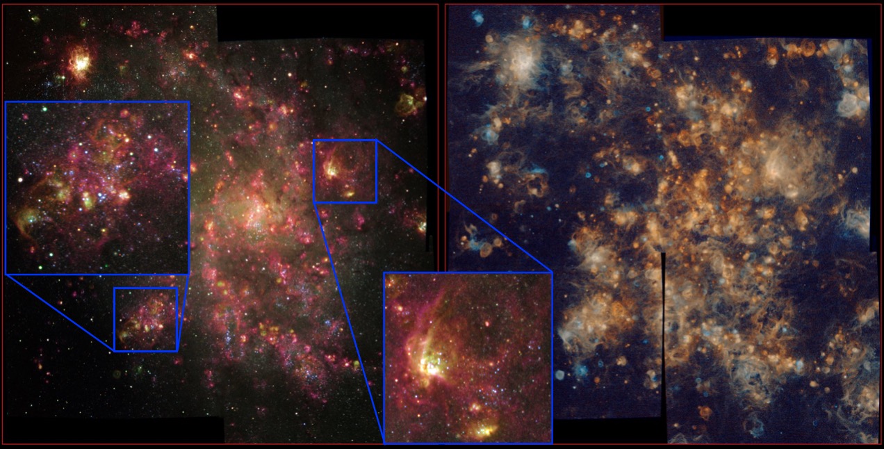
Figure 1: M33: SIGNALS’ science verification data (a mosaic of four fields). On the left, a composite image using the three filters . It combines the three continua over the wavelength range of the filters plus one emission line for each:  SN3+H$\alpha$ (red), SN2+[O III]$\lambda$5007 (green), and SN1+[O II]$\lambda$3727 (blue). The blue squares are zooms in two areas to show additional details. On the right, to emphasize the ionized gas component, we used the emission line map of H$\alpha$, [O III]$\lambda$5007, and [O II]$\lambda$3727 with different shades of orange, green, and blue, respectively.

SIGNALS, the Star formation, Ionized Gas, and Nebular Abundances Legacy Survey, is using SITELLE to observe more than 50 000 resolved extragalactic H II regions in a sample of $\sim$40 nearby galaxies over three spectral ranges (363 - 386 nm, 482 - 513 nm, and 647 - 685 nm). By studying the spatially-resolved spectra of individual H II regions and their massive stars content, SIGNALS’ main scientific objective focuses on how diverse local environments (nearby stellar population mass and age, dynamic structures, gas density and chemical composition, etc.) affect the star formation process. The legacy of this survey will also contribute to many topics in astrophysics, from stars to very distant galaxies. More specifically, the primary goals of SIGNALS are:

1) to quantify the impact of the surrounding environment on the star formation process;

2) to link the feedback processes to the small-scale chemical enrichment and dynamics in the surrounding of star-forming regions;  and

3) to measure variations in the resolved star formation rate with respect to indicators used to characterize high-redshift galaxies.

This paper presents an overview of the SIGNALS project observational strategy and data reduction (Section 2), galaxy sample (Section 3), science goal requirements (Section 4), data products (Section 5), and legacy value (Section 6).

2 Observations and Data Reduction

2.1 Strategy and Filter Configurations

SITELLE was designed to be optimized for the study of emission-line objects. A lot of technical challenges were overcome while building the instrument to assure excellent sensitivity, a high spectral resolution, and a large FOV (Drissen et al. 2019). SIGNALS’ observing strategy is built upon SITELLE’s unique capabilities. Three filters are used to optimize the detection and characterization of the strong diagnostic lines for nearby extragalactic nebulae:  SN1 (363 - 386 nm) with the [O II]$\lambda$3727 and the Balmer emission lines H9 to H12 (detected in bright regions), SN2 (482 - 513 nm) with H$\beta$ and [O III]$\lambda\lambda$4959,5007, and SN3 (647 - 685 nm) with H$\alpha$, [N II]$\lambda\lambda$6548,6583, He I$\lambda$6678, and [S II]$\lambda\lambda$6717,6731. These filters also provide a sampling of the continuum. Figure 1 shows an example of the deep images obtained combining the data from the three SIGNALS’ filters using two different methods for M33. This dataset was acquired for the science verification of the SIGNALS project and includes four fields. Figure 2 shows an example of an H II region spectrum in NGC628 obtained with SITELLE during its commissioning (Rousseau-Nepton et al. 2018). The main lines investigated by the survey are compiled in Table 1. The SITELLE Exposure Time Calculator (ETC) was used to simulate the expected signal-to-noise ratio (SNR) for specific lines and to define the instrumental configurations (i.e. spectral resolution, exposure time, and Moon maximal contribution). The ETC SNR calculation includes both the contributions of the sky and the target emission to the photon noise. The main driver for the configurations’ selection was the detection threshold (while avoiding saturation of the detector) over the range in surface brightness (SB) observed in H II regions, from $\sim$ 8 $\times$ 10^-17 to 8 $\times$ 10^-12 erg s^-1 cm^-2 arcsec^-2. Table 2 summarizes the parameters for the three selected configurations.

Table 1: Main emission lines for SIGNALS

Ion	Description
[O II]	[O II]$\lambda\lambda$3726,3729
H II	H$\beta$ (4861 Å)
[O III]	[O III]$\lambda$4959
[O III]	[O III]$\lambda$5007
[N II]	[N II]$\lambda$6548
H II	H$\alpha$ (6563 Å)
[N II]	[N II]$\lambda$6583
He I	He I$\lambda$6678
[S II]	[S II]$\lambda$6716
[S II]	[S II]$\lambda$6731

Table 2: Filter configurations

Filter	Band [nm]	Spectral Res.	Exposure time [sec step-1]	# of steps	Integration time [hours]
SN1	363-386	1000	59.0	172	3
SN2	482-513	1000	45.5	219	3
SN3	647-685	5000	13.3	842	4

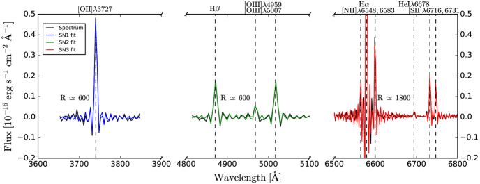
Figure 2: Continuum subtracted spectrum of an H II region in NGC 628 extracted from the datacubes using a circular aperture with a radius of 1.6^′′, centered at RA 01h36m53.1s and DEC +15^∘48^′04.8^′′. The fits obtained with ORCS (Sect. 5) for the emission lines are shown. Note that SITELLE’s line profiles are fitted using a cardinal sine function. Spectral resolutions obtained here are significantly smaller than those selected for SIGNALS.

The instrumental configuration for SN1 and SN2 was set using a spectral resolution of 1000, enough to separate the emission lines (the unresolved [OII]$\lambda\lambda$3726,3729 doublet; hereafter [OII]$\lambda$3727, [OIII]$\lambda$4959, [OIII]$\lambda$5007, and H$\beta$) and to properly measure the stellar continua. For the SN3 filter (648 - 685 nm), which contains the H$\alpha$ line broadly used to study gas dynamics, we adopted a higher spectral resolution of R = 5 000 in order to reach a precision on the velocity measurements of $\sim$0.1 to 10 km s^-1 (for H II regions with a SNR of 1000 to 10). With this configuration, we are also sensitive to velocity dispersion ranging from 30 km s^-1 for a faint region (over one seeing element) down to $\sim$ 10 km s^-1 for most of the regions observed and $\sim$ 1-2 km s^-1 for the brightest resolved regions. Figure 3 shows the relation between the minimum measurable broadening ratio of the Gaussian over the sinc functions used to fit a line of a given SNR. Appropriate binning can be used to reach a higher precision on the velocity measurements for kinematics studies (see Section 4.8).

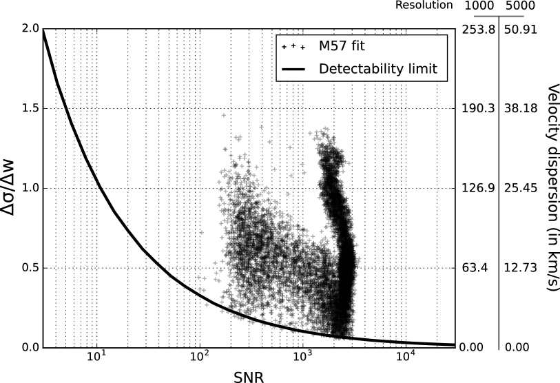
Figure 3: Instrument line spread function ratio. The black line shows the minimum measurable ratio $\Delta\sigma$ (observed) /$\Delta w$ (theoretical or pure sinc) for a line with a given SNR. The corresponding velocity dispersion at the two different resolutions used for SIGNALS (5000 and 1000) are reported on the right axis. It scales linearly with the resolution. A set of points from a fit of NGC6720 data with ORCS (Martin & Drissen 2017) is overlapped to the prediction. In this case, we can see that the SNR of the data points is high because all the lines in each spectrum are fitted with the same broadening parameter.

With these configurations, the detection thresholds (SNR $>\,$3) over an element of resolution of 1^′′ are SB_Hα $\simeq$ 3.6$\times$10^-17, SB_Hβ $\simeq$ 4.2$\times$10^-17, and SB${}_{\rm[O\,{\small II}]3727}$ $\simeq$ 3.0$\times$10^-17 erg s^-1 cm^-2 arcsec^-2 for SN3, SN2, and SN1, respectively. We used H$\alpha$, H$\beta$, and [O II]$\lambda$3727 as reference since they are the key lines of interest in their respective filters. Note that the threshold for H$\alpha$ corresponds to a SNR of 6.7 on the faintest H II regions and is also good for further investigation of the diffuse ionized gas (DIG, see Section  4.7) component at SB_HαDIG $\simeq$ 5$\times$10^-18 erg s^-1 cm^-2 arcsec^-2; additional binning may also be used later during the analysis. No extinction was applied on the ETC simulations but, adopting these numbers, we estimated that over 30% of the pixels detected in H$\alpha$ will have a H$\beta$ detection before applying any spatial binning. This is also supported by the relative detection we obtained on other galaxies during commissioning of SITELLE. After spatial binning, this detection threshold ensures that most H II regions will have a reliable measurement of the H$\alpha$/H$\beta$ ratio on the integrated spectra ($>$95%;  considering a mean extinction $E(B-V)$ $\simeq$ 0.5 and no background).

The current average seeing of the fields that have already been observed is 1.0^′′. The seeing of the observations is limited to a mean value of 1.2^′′ over a scan in order to maintain the global spatial sampling of the H II regions. Data observed with a mean seeing greater than 1.2^′′ are not validated. The moon contribution must be minimal for the blue SN1 filter. For the other two filters the moon contribution can be moderate (50% illumination and at a distance greater than 70^∘) without affecting the detection threshold significantly.

2.2 Data Reduction and Calibrations

Two software components have been developed specifically for the reduction and spectral analysis of SITELLE’s datacubes:  the data reduction software, ORBS and the data analysis software, ORCS (Martin et al. 2015, 2016).

ORBS is a fully automated data reduction pipeline, tailored for IFTS data, transforming the interferogram cube of SITELLE’s cameras into a spectral datacube. The first ORBS data processing step includes the wavelength calibration using a He-Ne laser datacube observed during the same observing run as the science datacube. As they come out of the reduction pipeline, datacubes have a pixel-to-pixel velocity error estimated to be of the order of 0.1 km s^-1 at R $=$ 5000. Additional correction is applied to the absolute wavelength calibration using the skylines centroid map as described in Martin et al. (2018) resulting in an accuracy of $\sim$1 km s^-1 on the measured relative velocities across the FOV (see appendix B of Martin et al. 2016 for details).

The first data processing also includes a correction of the zero, first, and greater than one phase orders as described in Martin & Drissen (2017). This ensures an instrument line spread (ILS) function that follows the theoretical model according to the selected instrument configuration. The ILS function for SITELLE is a pure cardinal sine (sinc) function. The FWHM of the sinc function is known and fixed since it depends only on the sampling and the maximum optical path displacement of the interferogram scan (Martin et al. 2016; Drissen et al. 2019). As shown in the work of Martin et al. (2016), when natural line broadening is observed, a sinc convolved with a Gaussian function can be used to properly recover the line parameters. If so, the line model has three varying parameters (amplitude, velocity, and broadening of the Gaussian). The uncertainty on the measurements depends on the SNR and the proper selection of the line model (sinc or sinc+Gaussian) and the set of lines to be fitted for each pixel (all lines must be fitted simultaneously, and if multiple components are present, they must be fitted simultaneously as well). As also described in Martin et al. (2018), the precision on the velocity obtained over the planetary nebulae in M31 ranged from 2 to 6 km s^-1 for sources of surface brightness much lower than what is expected for most H II regions.

The ORBS flux calibration uses flat images and standard star images taken during the same night as the science observation as well as standard star datacubes from the same observation run. The airmass is corrected using the atmospheric extinction curve above Maunakea provided by The Nearby Supernova Factory et al. (2013) and the mean airmass of the cube. Atmospheric extinction variations through a datacube are corrected using the transmission function extracted by normalizing the combined interferogram of the two output detectors to the maximum flux observed through the scan. Since a datacube is observed over a period of 3 to 4 hours and the transmission variations are corrected and normalized to the best transmission conditions seen during this period, the transmission variation is completely negligible. The flux calibration function itself is extracted from the standard star datacube using the star integrated spectrum in a given filter corrected for its own airmass and is used as a reference for the zero point correction. Zero point variations are tracked and corrected using the standard images taken during the night in photometric conditions. This data reduction procedure ensures a pixel-to-pixel relative flux calibration accuracy better than 2%. The datacube-to-datacube relative flux calibration accuracy is better than 5% (Martin & Drissen 2017), including both random and systematic errors. This will be improved in the second release of ORBS currently being developed for the SIGNALS program. Figure 4 shows the relative overlap between the SITELLE and the SDSS filters. Comparison with ancillary data can always be made to improve the flux calibration before the second data release.

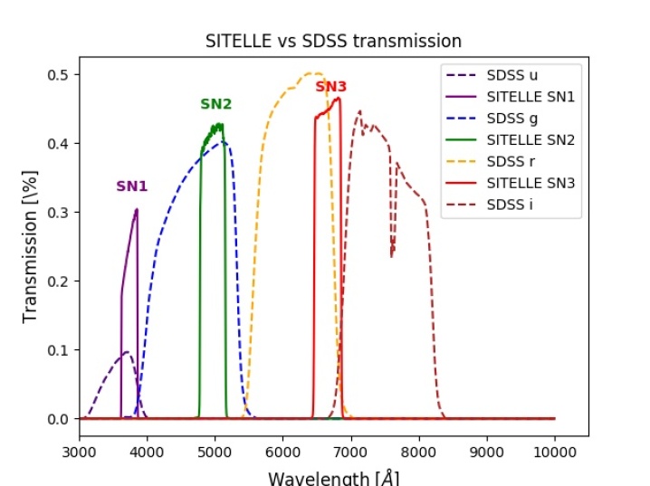
Figure 4: Transmittance curves for the atmospheric (airmass=1), telescope and optical assembly from SITELLE and SDSS. The SIGNALS filters (SN1, SN2, and SN3) are shown along with the overlapping SDSS filters.

3 Sample of H ii Regions

Our sample selection was driven by the need to observe a very large number of extragalactic H II regions in as many different galactic environments as possible. Star-forming areas within galaxies therefore motivated our choice. They were identified from existing H$\alpha$ and UV-GALEX images from all nearby galaxies observable by CFHT. To allow for a minimum contiguous observing period of 2 h from Maunakea with an airmass of 1.5 or smaller, targets with a declination below $-$22^∘ and over $+$62^∘ (i.e. the limits of the instrument) were rejected. The maximum galaxy distance was set to 10 Mpc in order to optimize the spatial resolution while still sampling a large number of H II regions. This ensures a spatial resolution of 40 pc per resolution element or less for a seeing of 0.8^′′. Our selection criteria can be summarized as$:$

1) star-forming galaxies;

2) $-$22^∘ $<$ DEC $<$ $+$62^∘;

3) D $\leq$ 10 Mpc;

4) limited amount of dust on the line-of-sight; and

5) limited crowding of the H II regions (inclination $\leq$ 71^∘).

Here crowding refers to observing multiple HII regions along the line-of-sight.

Based on these criteria, our sample of potential targets includes 54 objects. Except for some very large objects, most targets necessitate only one SITELLE field. As a result of the first criterion, some non-active areas and entire galaxies were rejected. For instance, galaxies such as the Cetus Dwarf Spheroidal and DDO 216, as well as the very outskirts of some extended galaxies (like M33) were excluded if they contained fewer than 10 regions within one pointing in order to increase our observing efficiency. To minimize the effect of internal dust extinction, we excluded massive, dusty, edge-on spirals from the sample (e.g. NGC 4631, NGC 4244, NGC 4605, etc.). However, we kept the foreground portion of the M31 disk. Table  3 contains the list of potential targets for the survey and a summary of their properties. Among this sample, 36 fields will be selected and observed with the SITELLE filters SN1, SN2, and SN3, for a total of 355 hours. By extrapolating from available H$\alpha$ images of the galaxies, the number of fields observed, and the known accuracy of the region identification as a function of spatial sampling, we estimate that about 50 000 H II regions will be analyzed. Each semester, an updated list will be published on the SIGNALS Website.

Other selection criteria should also guarantee the uniformity of the sampling of different galactic environments:  the oxygen abundance 12+log[O/H], varying from 7.5 in Sextans A (Kniazev et al. 2005) to $\geq$ 9.0 in objects like M51 and M63 (Pilyugin et al. 2004);  the stellar density (proportional to $\mu_{\rm V}$), ranging from $\mu_{\rm V}$ below 30 mag arcsec^-2 up to 18 mag arcsec^-2; the molecular and neutral gas mass,which is also very different between these galaxies; and galactic structures (size of the bulge, spiral arms, bars, rings, faint external structures, etc.). The objects selected are broadly distributed in mass with the addition of smaller irregular galaxies in order to sample different metallicities and environments with a similar statistical weight. The Hubble type and distance distribution of the sample is shown in Figure 5. The properties that were important for the completion of our sample can be summarized as follows$:$

1) global metallicity: 7.5 $\lesssim$ 12+log[O/H] $\lesssim$ 9.0;

2) magnitude: $-$21.3 $\lesssim$ M_absolute $\lesssim$ $-$13.5 mag;

3) surface brightness: 18 $\lesssim$ $\mu_{\rm V}$ $\lesssim$ 30 mag arcsec^-2; and

4) galactic environments: 1/3 isolated objects, 2/3 in groups, with no strongly interacting systems.

The group property of the galaxies was extracted from NED

As the data is analyzed, the selection can be adjusted to properly sample the different environments. For example, if we gather enough high metallicity and dense environment regions, we will then concentrate on the small irregular galaxies with a low-metallicity. We will prioritize the completion of the science goals and that depends mostly on the sample of H II regions and less on the completion of one particular target.

Among SIGNALS’galaxy sample, 7 targets are very close, resulting in a spatial resolution below 3 pc in the best observing conditions. A mosaic of several fields with small overlaps is used for these objects to cover most of the star-formation activity. Figure 1 shows an assemblage of four fields in M33 from the SIGNALS pilot project obtained in 2017. Reaching such a high spatial resolution is essential for some objectives of the project, i.e. to resolve gas ionization structures and the ionizing star content of the nebulae (e.g. faint end of the H II region luminosity function, calibration of the models with resolved structure of ionized gas, etc.).

The spatial resolution of the sample ranges from 2 to 40 pc. It should complement the MUSE survey over the northern sky (PHANGS/MUSE). Out of 19 galaxies, SIGNALS has 6 are in common with PHANGS/MUSE. We also compiled existing data from HST+LEGUS (28 galaxies), GALEX (UV, 39 galaxies), Spitzer (IR, 43 galaxies), BIMA and ALMA (CO, 23 galaxies), VLA (HI, 42 galaxies), as well as those obtained with narrow-band filters. These will be used to complete our analysis. The availability of this complementary data for the SIGNALS sample is also indicated in Table  3.

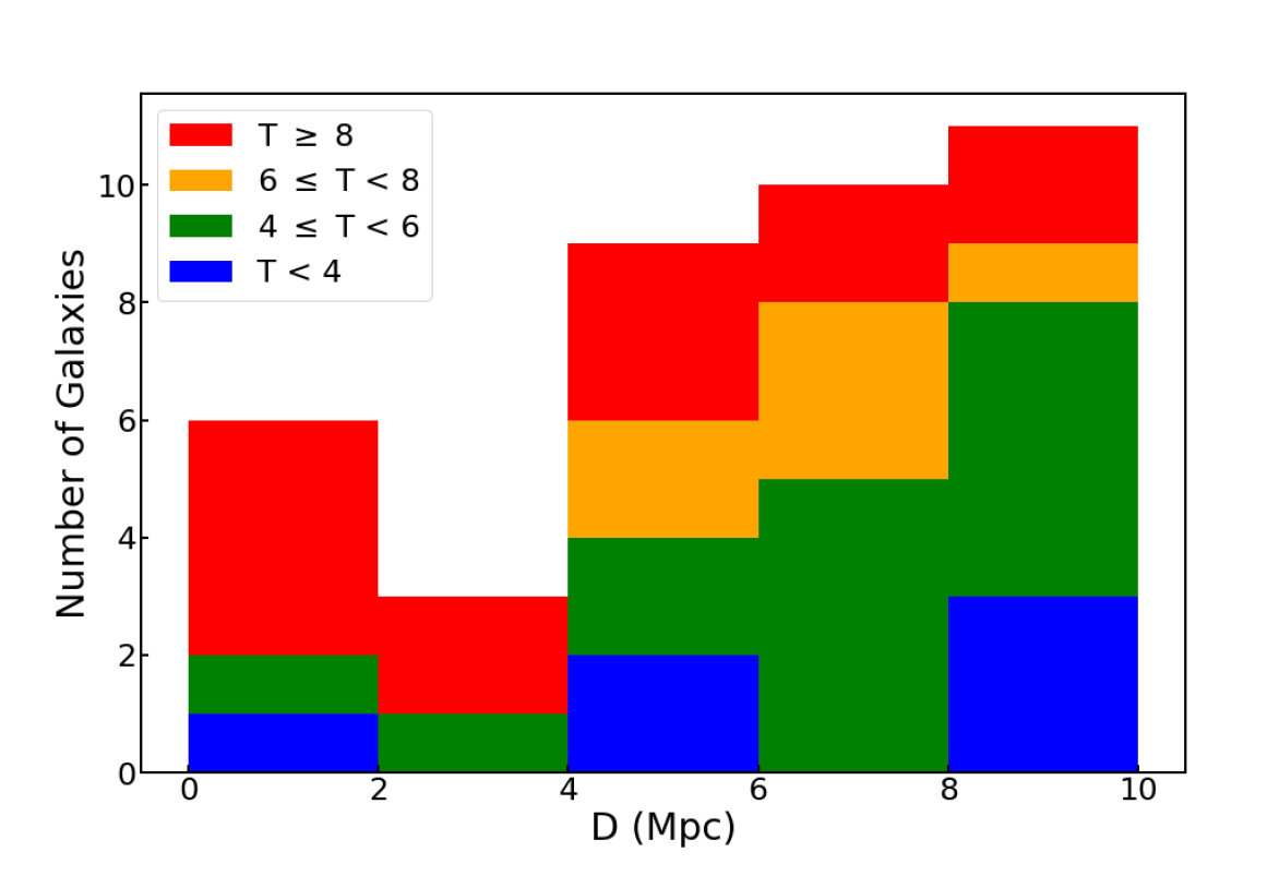
Figure 5: Distribution of the primary targets as a function of distance. The galaxies are color-coded according to their morphological type, as given by the parameter T from the revised Hubble classification scheme.

4 Science Requirements

SIGNALS aims to measure the strong emission lines while resolving individual H II regions. We also want to measure the H$\alpha$ brightness of the DIG, study small-scale dynamics of the gas and investigate feedback mechanisms at the scale of H II regions. As described in Section  2.1, the observation strategy was defined from basic constraints related to the detection of faint H II regions and the DIG with respect to their expected surface brightness and the known velocity dispersion observed in the ionized gas. The target selection was based on the spatial resolution requirement and the efficiency at observing a large number of H II regions in different local environments.

As described in this section, different steps resulting in the proper measurements of the emission line and continuum fluxes, as well as the velocity and its dispersion, were tested during the design of the survey:  1) an additional wavelength calibration for the velocity field is obtained by fitting the OH sky lines of the SN3 filter subtraction;  2) the sky subtraction is performed using sky sampling through each datacube;  and 3) the stellar continuum subtraction is applied pixel by pixel using a model for the stellar population. Finally, once the lines are properly measured, the analysis involves:  4) a dust correction using the Balmer decrement method;  5) the identification of emission regions ;  and 6) characterization using photoionization models. Requirements for meeting science goals on the study of:  7) the feedback processes;  8) the dynamics;  and 9) the impact of local environments, are also introduced in this section.

4.1 Wavelength Calibration using Sky Lines

As mentioned in Section 2.2, the wavelength calibration provided by the data reduction pipeline ORBS is performed by measuring the position of the laser line on a He-Ne datacube through the FOV, and applying the measured centroid map to scale the science cube spectral axis (Martin & Drissen 2017). Some velocity residual errors remain from this technique since the science observations are made at different on-sky positions than those of the calibration laser (zenith). As described in Martin et al. (2016) and Martin et al. (2018), the sky lines observed in the SN3 filter can be used to correct residual errors. A simultaneous fit of all the bright sky lines available in the bandpass is made using the ORCS analysis tool. The resulting velocity map is interpolated over the FOV and a correction map is then applied to any subsequent velocity map extracted from the emission line with ORCS. Note that at R $=$ 5000, the sky lines are well resolved and their number reduces the uncertainties on the velocity extracted from the fit. The same accuracy is not required for the SN1 and SN2 filters.

4.2 Sky Subtraction

The sky subtraction is performed on each pixel using a high SNR sky spectrum built from each datacube. This sky spectrum is extracted using the median of the available sky spaxels over the FOV. Although a few hundred pixels is enough to produce such a spectrum which corresponds to an area greater then $\sim$10 arcsec² on the sky, all the available sky spaxels can be used to produce the median sky spectrum. The selection of those sky spaxels is made from the deep image of the datacube (the deep image is the image produced from the stacked datacube along the spectral axis) by defining a maximum threshold on the image intensity. This threshold can be adjusted from one target to another to optimize the selection of the faintest pixels while still using a large number of them. This adjustment is important to minimize the DIG or stellar background contamination to the sky spectrum. We estimate that the vast majority of all SIGNALS fields will have enough sky sampling to perform the high SNR sky spectrum subtraction (i.e. at least 10 000 sky spaxels corresponding to a SNR $\geq$ 100). For pointings without any pixels enabling the sampling of the sky, we use a model of the sky spectrum obtained by fitting the bright lines with ORCS. Since the emission of the sky can vary in time and since it includes a faint H$\alpha$ component, a model is used only when a high SNR sky spectrum cannot be produced.

4.3 Stellar Continuum Subtraction

The stellar population contribution to each spaxel is subtracted to obtain the proper emission line fluxes. At the SIGNALS spatial resolution of 2 to 40 pc, the effect of stellar continuum subtraction is much smaller than at resolutions of 1 kpc. The emission of the gas is concentrated in clumpy areas while the stellar population in massive galaxies is more uniformly distributed. For example, at a $\mu_{\rm V}$ $=$ 18 mag arcsec^-2, the intensity of the continuum is of 2.65$\times$10^-17 erg s^-1 cm^-2 Å^-1 arcsec^-2 which corresponds to 2.71$\times$10^-18 erg s^-1 cm^-2 Å^-1 pixel^-1. Note that this level corresponds closely to the level of noise in one spaxel for any given SIGNALS datacube. For low-mass galaxies, no continuum subtraction is necessary for our project. Nevertheless, the continuum can dominate the emission in the central part of massive galaxies. To properly measure the emission from faint H II regions or the DIG components in those areas (SB_HαDIG $\simeq$ 5$\times$10^-18 erg s^-1 cm^-2 arcsec^-2), a subtraction of the stellar population background needs to be performed.

As shown in Rousseau-Nepton et al. (2018), a stellar continuum can be extracted directly from the datacubes. At a resolution of R $=$ 5000, the stellar absorption line can be fitted along with the emission line. This is important for the H$\alpha$ and H$\beta$ absorption lines. For the galaxies observed in SIGNALS, the stellar population continuum subtraction will be performed in three steps:  1) a fit of the gas emission will be performed to obtain an estimate of the velocity field, the emission line fluxes, and the continuum level, 2) the aperture for the stellar continuum sample will be defined using the galaxy luminosity profile, 3) the stellar population spectra will be extracted or fitted through the apertures and used to subtract the component from each spaxel (e.g. Moumen et al. 2019). Ideally, when the SNR and spatial resolution allow it, the local environment will be used to build the galaxy background spectrum directly from the datacubes. While selecting the pixels to build the stellar continuum spectra, a limit on the combined emission line map flux (from a preliminary fit of the emission with ORCS) is used to exclude pixels with a significant contribution from the DIG and/or surrounding HII regions. If no pixel passes this selection test, or if the noise level of the stellar continuum spectrum is higher than 1/10 of the detection threshold for the HII regions, the aperture is increased. Depending on the galaxy, this method will not always be possible and other ones will be considered.

Also discussed in Rousseau-Nepton et al. (2018), although some pixels within an emission region may be affected by the young population continuum flux and absorption lines, our method for the subtraction of a local or global background stellar population spectrum takes into account most of the young population emission. Indeed, when the stellar population spectrum is subtracted, it is first rescaled to the continuum level of the emission region, which takes into account the continuum level of the young population. The absorption line profiles in this rescaled stellar population spectrum do not contain the exact contribution from the young population, but this inaccuracy is negligible compared to the final noise level in the emission lines. Tests done with a combination of model spectra for young and old populations with different ages and proportions support this idea.

4.4 Dust Extinction Correction

The dust extinction contribution is included in our model for the spectral analysis. To provide dust corrected fluxes, the extinction law of Cardelli et al. (1989) is used and the color excess ${E(B-V)}$ is evaluated from the known equation:

$$E(B-V)\,=\,\frac{2.5}{1.10}\log\left[\frac{({\rm F}_{{\rm H}\alpha}/{\rm F}_{{\rm H}\beta})_{\rm obs}}{({\rm F}_{{\rm H}\alpha}/{\rm F}_{{\rm H}\beta})_{\rm theo}}\right],$$ (1)

with $({\rm F}_{{\rm H}\alpha}/{\rm F}_{{\rm H}\beta})_{\rm theo}$ given by the photoionization models, and $E(H\beta-H\alpha)$/$E(B-V)$ = 1.10.

Measured fluxes, both corrected and uncorrected for the dust extinction, will be provided in the catalog of H II regions (see Section 5).

4.5 H ii Region Identification

To separate individual H II regions, a spatial resolution of the order of 10 pc is required. Figure  9 from Kollmeier et al. (2017) illustrates how the ionized gas structures and individual clumps of star formation can be resolved by increasing the spatial resolution. Below a resolution of 50 pc, observations reveal structures in the ISM including individual star-forming knots, DIG, and shocks. The filling fraction of the observations are also important for analyzing the gas photoionization conditions. Figure  6 shows the impact of the FOV and filling-factor on the H II region spectrophotometry by comparing the log([N II]$\lambda$6583/H$\alpha$) maps obtained with SITELLE and the CALIFA PPAK IFU survey (filling factor $\sim$ 60$\%$, Rosales-Ortega et al. 2011). The maps differ significantly. Notably, the flux of faint areas covered by fibers (for fiber-fed systems) becomes negligible resulting in a total flux per resolution element dominated by the brightest zones. Areas not covered by fibers do not contribute to the resulting map.

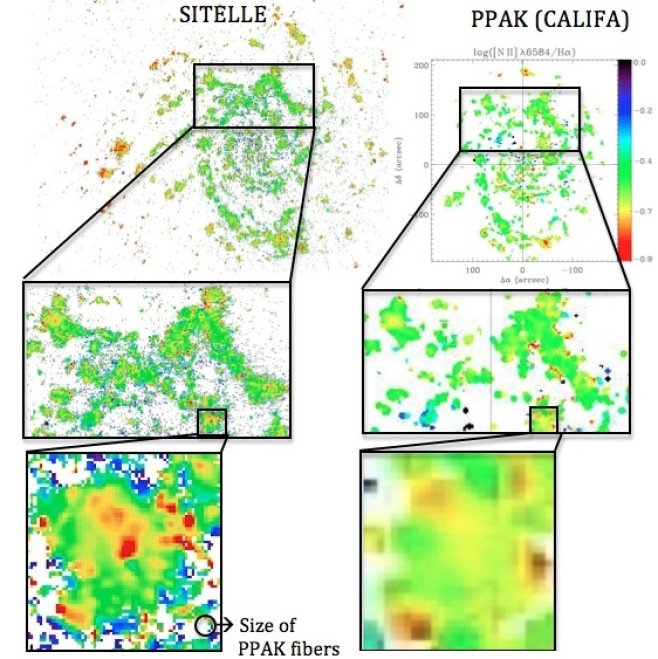
Figure 6: Spatial resolution and filling factor impact on the measurements of emission line ratios. The line ratio log([N II]$\lambda$6583/H$\alpha$) extracted from SITELLE’s observations on NGC 628 (0.8^′′ seeing, 0.32^′′ per pixel, 100% filling factor) is compared to PPAK’s observations on the same area (0.8^′′ seeing, 2.7^′′ per fiber, 60% filling factor). The color scale is the same for both maps (upper-right corner). The PPAK map (on the right) is published in Rosales-Ortega et al. (2011) and was re-used here for comparison purpose only.

Our analysis of the science verification data allowed us to identify 4285  H II region candidates in NGC 628 using a tailored procedure developed for the SITELLE data at a spatial resolution of 35 pc. Details are published in Rousseau-Nepton et al. (2018). There are two advantages of the IFTS that our procedure uses:  the full spatial coverage and the spectral information. By combining the flux of three emission lines (H$\alpha$, H$\beta$, and [O III]$\lambda$5007), we increased the detection threshold and improved the detection of the low metallicity regions with much fainter recombination lines. This code provides flexibility in defining the regions and their DIG background. Our method proceeds through multiple steps:  1)the identification of the emission peaks;  2) the determination of the zone of influence around each peak;  and 3) the definition of the outer limit of a region and its DIG background. Figure 7 shows the border of a few H II regions derived from this procedure. For SIGNALS, it will be adapted to different spatial resolutions to make sure that the regions are uniformly defined. SITELLE’s dataset for NGC 628 was used to recover the luminosity function for different samples of H II regions as shown in Rousseau-Nepton et al. (2018). These luminosity functions, established from 2000 - 4000 regions, are well sampled and provide interesting insights on the active star formation processes within that galaxy.

Figure 7: Examples of ionizing sources and their zone of influence in NGC 628 drawn over the H$\alpha$ + H$\beta$ + [O III]$\lambda\lambda$4959,5007 continuum-subtracted image from Rousseau-Nepton et al. (2018). The centroid position of each emission peak detected is identified with a cross. The white contours define the zones of influence surrounding the emission peaks.

4.6 H ii Region Characterization

Photoionization models are usually employed to understand the physical properties of H II regions, whether or not their ionization structure is resolved, e.g. CLOUDY (Ferland et al. 1998; Morisset et al. 2015) or MAPPINGS (Dopita & Sutherland 1995; Ho et al. 2014). The ensemble of emission lines listed in Table 1 will allow us to investigate a broad range of physical conditions for the gas and ionizing sources (Kewley & Dopita 2002; Pérez-Montero et al. 2014; Vale Asari et al. 2016). With those lines (and their ratios), we are planning three different modeling strategies for SIGNALS:  Integrated Spectra Modeling, Spatially Resolved Modeling, and Modeling the Populations.

4.6.1 Emission Line Detection

The intensities of the strong nebular lines vary with the physical conditions in the gas. Nevertheless, we can make some assumptions about the detectability of the strong lines from previous observations and grids of photoionization models. When a line is not detected, the detection threshold adds a constraint on the line???s flux which can still be used to narrow down the region’s physical conditions. Depending on the region size and the spatial resolution, the detection threshold changes and this effect has to be considered as an observational bias in the subsequent analysis.

For nearby targets, most regions will be spatially resolved and multiple spaxels will be available to increase the detection limit. For the faintest regions, considering a surface brightness of $\sim$ 8 $\times$ 10^-17 erg s^-1 cm^-2 arcsec^-2 and a radius of 2^′′, a SNR of 3 would be reached for any line with a flux greater than 12% of H$\alpha$ (or log[line/H$\alpha$] $\geq$ $-$0.9). For any region with a surface brightness greater than 3.4 $\times$ 10^-16 erg s^-1 cm^-2 arcsec^-2 and a radius of 2^′′, a SNR of 3 would be reached for any line with a flux greater than 3% of H$\alpha$ (or log[line/H$\alpha$] $\geq$ $-$1.5). According to photoionization models (Vale Asari et al. 2016), this corresponds to virtually all the regions for [N II]$\lambda$6583, [S II]$\lambda\lambda$6716,6731, and [O II]$\lambda$3727. Figure 8 shows the expected ratios of the strong lines over H$\alpha$ for a set of models from the Bayesian Oxygen and Nitrogen abundance Determinations database (BOND, Vale Asari et al. 2016) including models for ages ranging from 1 to 6 Myr, optical depth of 1.0, log[N/O] ranging from 0 to $-$2.0, 12+log[O/H] ranging from 6.5 and 9.5, and ionization parameters ranging from $-$2.5 to $-$4 (value observed in the CALIFA sample, Morisset et al. 2016). We can see that within the range of metallicity expected for the extragalactic H II regions of the sample, all models show strong lines’ relative intensities $\geq$ $-$1.5. For [N II]$\lambda$6583, we considered only regions with a log[N/O] above $-$1.5, since H II regions are not observed frequently below that threshold (Berg et al. 2015; Croxall et al. 2015, 2016). It is important to note that for [O III]$\lambda$5007, some cases will not detected, i.e. regions older than 5 Myr or with a low ionization parameters ($\leq$ $-$3.5). Note that in both cases the regions are fainter compared to others since the ionizing photons come from late B star(s). Nevertheless, not detecting the [O III]$\lambda$5007 line is a good constraint for the models. From the whole sample of spatially resolved H II regions (2-15 pc), a good fraction of them will have strong emission lines detected along the region profile, useful for our detailed 2D analysis (see Section 4.6.3).

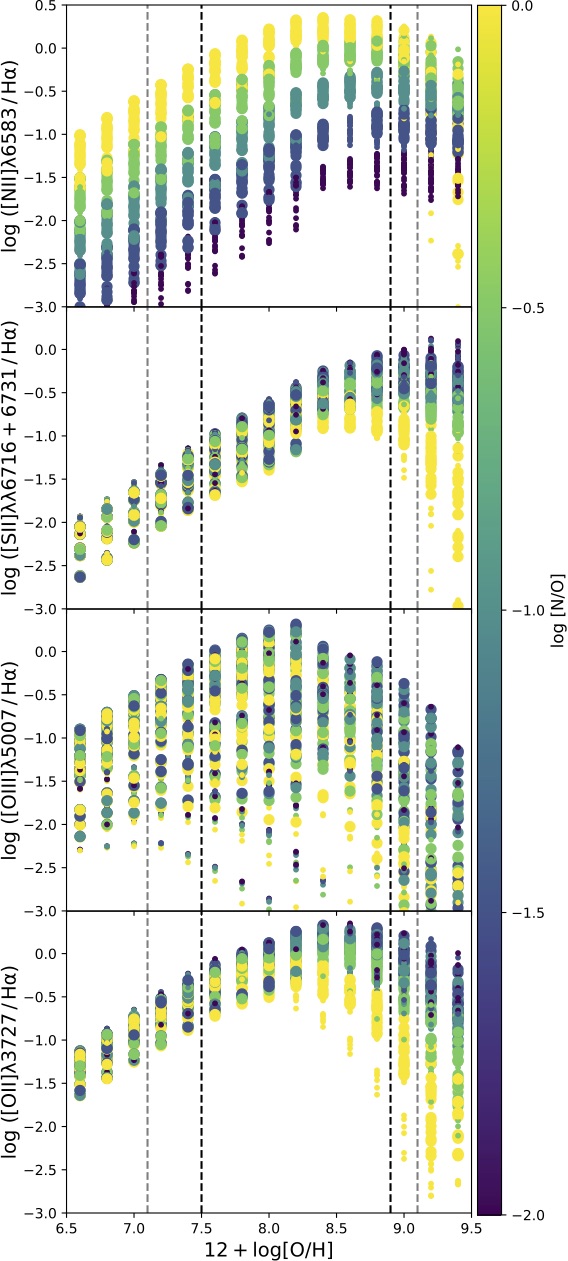
Figure 8: Prediction of several strong line ratios ([line]/H$\alpha$) of the CLOUDY photoionization code (extracted from the BOND grid of models on 3MdB). The color scale represents the log[N/O] ratio for a given model. The smaller dots correspond to models representing less expected regions (log[N/O] $<$ $-$1.5 or age $>$ 5.1 Myr or log[U] $\geq$ $-$3.55). The grey dashed vertical lines show the expected range of metallicity of the regions sampled and the black dashed vertical line shows the usual range of metallicity for most regions in the local Universe.

For further-away targets, we can approximately estimate the number of regions for which we will detect strong emission lines by comparing model predictions with observations. Two parameters mainly influence the detection of emission lines for unresolved regions$:$  the size distribution of the regions with respect to the resolution of the data, and the SB distribution of regions with respect to their size. Some small and faint regions cannot be detected in targets near the distance limit of the SIGNALS sample. Their flux is diluted in the resolution element. In the commissioning data of NGC 628, located at 9 Mpc, our measured detection threshold for H$\alpha$ was of 4.6 $\times$ 10^-17 erg s^-1 cm^-2 arcsec^-2 (slightly lower than for SIGNALS). Figure 9 shows the measured peaks’ SB function (histogram of the SB of the central pixel) of the regions detected with the identification procedure (Rousseau-Nepton et al. 2018) for different subsets of regions on NGC 628 for which there is a detection of a different strong line. From the regions detected with H$\alpha$, 84% were also detected in [N II]$\lambda$6583, 91% in [S II]$\lambda\lambda$6716+6731, 63% in [O III]$\lambda$5007, 84% in H$\beta$, 63% in [O III]$\lambda$5007, and 63% in [O II]$\lambda$3727. Part of the lower detection of the [O II]$\lambda$3727 line is due to dust extinction, a total exposure time of 2.13 hours (lower than for SIGNALS), and the loss of reflectivity of the telescope primary mirror (only a few months before realuminizing). For [O III]$\lambda$5007, about 5% of the regions were at a metallicity too high to be detected and, as mentioned before in this section, the other non-detected regions could be older than 5 Myr and/or they have a low ionization parameter. From the distance of NGC 628 to the closest target of the sample, the fraction of detected lines increases as more pixels are available to extract the spectra. NGC 628 is therefore a worst-case scenario for the detection of the lines.

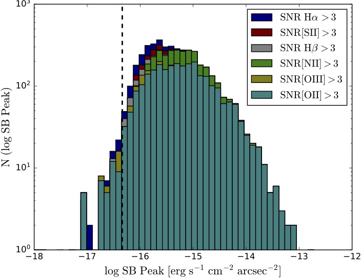
Figure 9: Surface brightness (SB) function of the H II regions in the commissioning data of NGC 628. The black dashed line shows the detection threshold of one element of resolution in H$\alpha$. The different colors represent selected subsets of regions for which there is a detection of different strong lines (see the legend). The few regions below the black dashed line are faint H$\alpha$ regions detected from the combination of H$\alpha$, H$\beta$ and [O III]$\lambda$5007 used for the identification.

4.6.2 Integrated Spectra Modeling

Grids of models covering different physical properties from various photoionization codes (BOND, Vale Asari et al. 2016;  3MdB, Morisset et al. 2015;  and MAPPINGS, Dopita & Sutherland 1995) will be compared to the SIGNALS’ H II regions integrated spectra. These grids are designed to study the effect of variations in the gas conditions on the integrated spectrum (region by region). Figure 10 shows an example of the comparison of emission line ratios observed in NGC 628 (Rousseau-Nepton et al. 2018) with BOND.

Different models can account for variations in the spectral energy distribution (SED) of the source, the metallicity [O/H], and the relative abundances of elements (e.g. [N/O]). The accuracy of the comparison with models can be improved by using a set of regions for which the ionization sources have been observationally constrained, e.g. Legacy ExtraGalactic UV Survey (LEGUS, Calzetti et al. 2015; Grasha et al. 2015). LEGUS provides access to both individual stars (Sabbi et al. 2018) and stellar cluster catalogues (Adamo et al. 2017). It also contains a fairly complete census of the massive stars (down to 15 M_⊙) and very young clusters (down to 10³ M_⊙). Thus, the combined data from SIGNALS and LEGUS will provide a better view of the H II region physics for a large fraction of our sample.

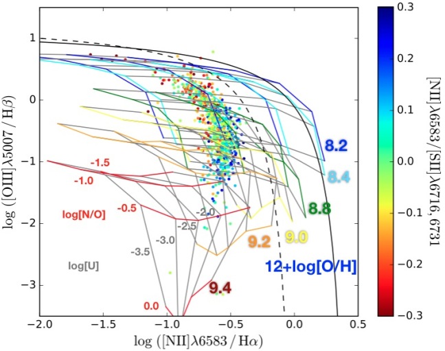
Figure 10: BPT diagram (Baldwin et al. 1981) of emission line regions identified in NGC 628 (from Rousseau-Nepton et al. 2018) along with a grid of models from BOND (Vale Asari et al. 2016) using the SED of a 3 Myr old stellar cluster with a Chabrier IMF (Chabrier 2003). The colors of the grids indicate different metallicities (12+log[O/H]). Horizontal lines have different values of log[N/O], as given in red for 12+log[O/H] = 9.4, and vertical lines have different values of log[U], as given in gray for the same metallicity. The color-scale of the scattered observational points indicates the log([N II]/[S II]$\lambda\lambda$6716+6731) line ratio which is known to be a good indicator of log[N/O] (Pérez-Montero et al. 2014). The limit between the H II regions and the transition regime (Kauffmann et al. 2003) is shown by the dashed curve, and the extent of the starburst domain (Kewley et al. 2001), is displayed by the continuous curve.

4.6.3 Spatially Resolved Modeling

When a H II region is resolved, spatial variations of the ratios as a function of the distance to the source of ionization are expected. This can be due to the varying photoionization conditions in the gas as the intensity and slope of the ionizing spectrum, temperature, and density change. Once integrated, the variations can be less apparent (e.g. [NII]/[OII] ratio, see Figures on p.37 of Rousseau-Nepton at al. 2018).

The 2D sampling of the line emission enables the use of multi-dimensional photoionization models to constrain gas properties (Wood et al. 2005, 2013; Weber et al. 2015; Rahner et al. 2019). For each source identified, we establish a mean profile of the line ratios as a function of the distance to the ionization source (OB stars in the case of H II regions). These profiles along with the integrated flux of each line are needed to conduct a fair comparison with the models. Figure 11 shows a comparison of four line ratios with a 2D projection of the pseudo-3D model extracted from pyCLOUDY (Morisset 2013).

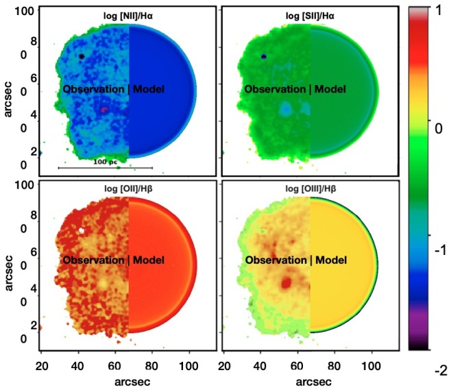
Figure 11: Comparison of a giant H II region observed with SITELLE in NGC 6822 with a 3D photoionization model projected on 2D images. The region is split in two for each panel:  the left side represents the observations while the right side is the model (a slice perpendicular to the line of sight that goes from the center of the region to the outskirts). A pure 40 000 K Planck function was used as ionizing spectrum and abundances at 20% of the solar value, excepted for S. The model was also for a thin shell of gas with log[U] = $-$2.6.

4.6.4 Modeling Populations

In addition to the region-by-region analysis, a statistical approach is used to study populations of H II regions. Figure 12 shows simulations of line ratios when combining photoionization models with evolutionary tracks of a population of star-forming clusters at solar metallicity. The emission measure predictor code WARPFIELD (Winds And Radiation Pressure:  Feedback Induced Expansion, colLapse and Dissolution, Rahner et al. 2017, 2019; Pellegrini et al. 2019) was used to produce Figure 12. WARPFIELD considers a semi-analytic model to describe the impact of mechanical and radiative feedback from a young massive cluster on its parental cloud. Its approach simultaneously and self-consistently calculates the structure and the expansion of shells driven by feedback from stellar winds, supernovae, and radiation pressure, while accounting for the deceleration of the shell due to gravity. The model has been used to investigate the conditions under which the different sources of feedback dominate and the amount of radiation that escapes through the shell. It was also used to derive the minimum star formation efficiency for a large parameter space of clouds and clusters (Rahner et al. 2017). The same approach was used to explain the two stellar populations in NGC 2070 in the LMC, which hosts the younger cluster R136 in its center (Rahner et al. 2018). Because this method is computationally very efficient, it will allow us to consider a large range of parameters. We are currently compiling a comprehensive database where we vary the star formation efficiency, the cloud mass and density profile, and the metallicity of both the gas and the stars. Each model is currently being post-processed using CLOUDY to make detailed predictions for the time evolution of the line and continuum emission associated with the system. Using this code, we can build synthetic BPT-like diagrams for the one-to-one comparison with observational data, as shown in Figure 12.

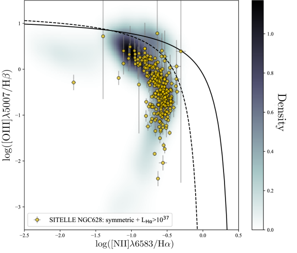
Figure 12: BPT diagram (Baldwin et al. 1981) of emission line regions identified in NGC 628 from Rousseau-Nepton et al. (2018), using circular regions only, along with simulations from CLOUDY using post-processing of evolutionary tracks from the WARPFIELD code (Rahner et al. 2019; Pellegrini et al. 2019). It combines a series of WARPFIELD runs with different cloud masses, densities, and ages. The color-coding indicates the relative number of model outputs used to produce a line ratio. See the caption of Figure 10 for the curve definitions.

4.7 Feedback Processes

Massive OB stars in H II regions are not only responsible for ionizing the surrounding gas but also for exerting direct radiation pressure onto this gas. They also return enriched material and mechanical energy through their stellar winds and supernova explosions to the ISM. While the efficiency of stellar winds involved in shaping an H II region bubble is still uncertain, it is possible that radiation pressure may play a dominant role at a younger age, while thermal pressure of the warm ionized gas may become more important at a later age (Lopez et al. 2014; Pellegrini et al. 2019). Also, the DIG can be observed near H II region boundaries. Recent works on the DIG have helped to quantify its emission in nearby galaxies (Lacerda et al. 2018; Poetrodjojo et al. 2019; Moumen et al. 2019) and photoionization models have been developed to trace back the spectral energy distribution of the source of ionization. Several sources of ionization might be responsible for the DIG: ionizing photons escaping H II regions that travel long distances (Ferguson et al. 1996; Haffner et al. 2009; Zurita et al. 2000; Oey et al. 2007; Barnes et al. 2014; Howard et al. 2016, 2017), a weak AGN (Ho 2008; Davies et al. 2014), a generation of post-AGB stars (Binette et al. 1994; Flores-Fajardo et al. 2011), and fast shocks in the ISM (Allen et al. 2008; Hoffmann et al. 2012). Some studies have suggested that only OB stars could be responsible for most of the DIG emission (Domgorgen & Mathis 1994). Others have found that a mix of multiple sources could explain the observed line ratios in the DIG (Weber et al. 2019; Poetrodjojo et al. 2019).

Detailed numerical simulations predict that the fraction of escaping photons varies considerably over a few million year timescale. Semi-analytic feedback models for the cloud dissolution (Rahner et al. 2017) have demonstrated that the SFE is linked to the ionizing escaping photons (i.e. a high SFE corresponds to a high fraction of escaping photons). Also, depending on the evolution phase of the H II region, the escaping photon fraction can change (Pellegrini et al. 2019). SIGNALS will measure the DIG surrounding each H II region as shown in Rousseau-Nepton et al. (2018). By measuring the relative contribution of the H II regions to their surrounding DIG, we will get precise constraints on the fraction of radiation and hot gas escaping the regions that merges with the low density ISM.

Our requirements for the study of feedback processes rely on:  1) the spatial resolution to resolve regions, filaments, supernova remnants, etc.;  2) the depth of the observations to detect faint regions and DIG emission;  and 3) the line ratios to track the ionizing front or its absence around H II regions along with the variation of chemical abundances in the gas. These requirements have already been met by the need to identify and characterize H II regions.

4.8 Kinematics and Dynamics

The spectral resolution provided by SITELLE SN3 cubes for five lines simultaneously (R = 5 000 for the H$\alpha$, [N II]$\lambda\lambda$6548,6583, and [S II]$\lambda\lambda$6717,6731 emission lines) will allow us to determine the line centroid (ORCS;  see Section 2.2) with a precision of 0.1 to $\sim$10 km s^-1 across the FOV. This will enable the detection of line broadening larger than 10 km s^-1 in most H II regions (see Figures 3 and 13). It will also separate multiple components along the line of sight (Martin et al. 2016). Combined with the line ratio analysis discussed in the previous subsections, several aspects of the ionized gas dynamics will be probed:  1) shell expansion velocity in H II regions, from which their mass can be determined;  2) random and rotational motions as a function of location in the disk (e.g. spiral arms versus interarm regions and DIG);  3) azimuthal anisotropy of random motions in the disk plane;  4) kinematics and abundance patterns linked to the mixing mechanisms and abundance variations (Sánchez-Menguiano et al., 2016);  5) kinematics of the ionized gas compared;  and 6) mass distribution models (Kam et al., 2017). In a few objects, the kinematics of the stellar halo should also be probed through the [O III]$\lambda$5007 emission line in PNe, allowing alternative derivations of rotation curves and mass profiles.

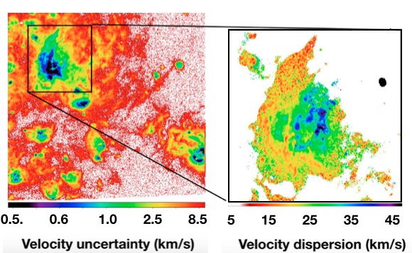
Figure 13: M33 H$\alpha$ velocity uncertainties and dispersion for a small portion of the SITELLE FOV with $R\,=\,3\,000$.

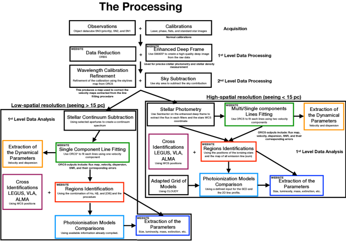
Figure 14: Organizational chart for the data processing. All items with the label WEBSITE will be accessible to everyone via our Website (http://www.signal-survey.org) once the collaboration team has analyzed the data and published the different catalogs. Note that all observed datacubes are available at the Canadian Astronomical Database Center (CADC).

4.9 Impact of Local Environment

To investigate possible relations between star-forming regions and their environment, the following parameters will be studied:  the local stellar density, local DIG background, local neutral gas density, local SFR and SFE, distances to the nearest regions, and location with regards to prominent galactic structures (bar, spiral arm, ring, AGN, etc). The size, geometry, and total H$\alpha$ luminosity will also be considered. A large variety of galaxies with different stellar populations and stellar densities can be found within the SIGNALS sample. Within each individual target this distribution also changes dramatically from one area to another. While the diversity of targets adds complexity to the analysis, it makes the analysis robust because reliable subsamples can be used for specific purposes in addressing the main goals of the project.

5 Data Products

Figure 14 summarizes the diverse processing steps presented in this paper, from the observational phase to the extraction of the physical parameters. The process differs between nearby (i.e. spatial resolution $\lesssim$ 15 pc) and more distant targets. The ORCS software can simultaneously or individually fit lines in each datacube while returning maps for each line including the amplitude, FWHM, continuum height, flux, velocity, velocity dispersion, and their corresponding uncertainties. The H II regions identified with our procedure will be included in a catalog that will contain the raw emission line measurements from the datacubes obtained after data processing and the stellar continuum subtraction. The median profile of each line will also be fitted as in Rousseau-Nepton et al. (2018); the fitting parameters will be provided in the catalog. Extinction corrected values will also be provided as explained in Section 4.4. The absolute position (right ascension and declination) of the center of each region will be provided as well as the name of the host galaxies. Additional data products extracted from complementary data will be added to the catalog when available (e.g. the mean $\mu_{\rm V}$ around the regions, and the total HI and CO emission evaluated over the region radius).
Data products will be distributed to the collaborators and other communities from the SIGNALS Website. The HDF5 files containing the reduced datacubes are available without any proprietary period from the program 18BP41, 19AP41, …P41, etc, via the Canadian Astronomy Data Centre Website. Data release of additional products following the analysis will be made available later from the SIGNALS Website.

6 Legacy Value

SIGNALS fills the gap between other galaxy surveys focusing on the local Universe, from the upcoming SDSS-V LVM survey to current surveys such as MAD, PHANGS, CALIFA, SAMI, MANGA, etc. It will provide new, key insights into star formation and feedback mechanisms driving the evolution of the ISM in star-forming galaxies. By using multiple nebular lines, physical properties like abundances, ionization structures, and dynamics will be obtained as well as information on the impact of local environments on the star formation process.

The rich SIGNALS dataset will be valuable for investigating other complementary astrophysical topics. Some possibilities include:  1) planetary nebula abundance distributions and luminosity functions (Kreckel et al. 2017; Martin et al. 2018);  2) supernova remnant ionization conditions, occurrence, and feedback contribution (Moumen et al. 2019);  3) detection of background emission line objects (e.g. [O II] and Ly-$\alpha$ emitters);  and 4) large-scale velocity mapping of galaxies. The SIGNALS collaboration team will make this dataset available to the scientific community, provide catalogs and diagnostic tools.

AFFILIATIONS
¹ Canada-France-Hawaii Telescope, Kamuela, HI, United States
² Department of Physics and Astronomy, University of Hawaii at Hilo, Hilo, HI, United States
³ Département de physique, de génie physique et d’optique, Université Laval, Québec, QC, Canada
Centre de Recherche en Astrophysique du Québec
⁴ Aix Marseille Univ, CNRS, CNES, LAM, Marseille, France
⁵ Department of Astronomy, The Oskar Klein Centre, Stockholm University, Stockholm, Sweden
⁶ Instituto de Astronomia, Universidad Nacional Autonoma de Mexico, Apdo. postal 70???264, Ciudad Universitaria, Mexico CDMX 04510, Mexico
⁷ Department of Physics and Astronomy, University of Western Ontario, London, ON, Canada
⁸ Institute for Astronomy, University of Hawaii, Honolulu, HI, United States
⁹ 2Sub-department of Astrophysics, University of Oxford, Denys Wilkinson Building, Keble Road, Oxford, United Kingdom
¹⁰ Centro de Astronomía, Universidad de Antofagasta, Avda. U. de Antofagasta 02800, Antofagasta, Chile
¹¹ Departamento de Física???CFM, Universidade Federal de Santa Catarina, Florianópolis, Santa Catarina, Brazil
¹² LERMA, Observatoire de Paris, PSL Research Univ., CNRS, Université de Sorbonne, UPMC, Paris, France
¹³ Coll??ge de France, 11 Pl Marcelin Berthelot, 75005 Paris
¹⁴ Institute of Astronomy, the University of Tokyo, Tokyo, Japan
¹⁵ Universitát Heidelberg, Zentrum für Astronomie, Heidelberg, Germany
¹⁶ Observatoire de Genève, Université de Genève, Sauverny, Switzerland
¹⁷ Instituto de Astronomia, Universidad Nacional Autonoma de Mexico, Ensenada, B.C., Mexico
¹⁸ Max Planck Institute for Astronomy, Heidelberg, Germany
¹⁹ Research School of Astronomy and Astrophysics, Australian National University, Canberra, Australia
²⁰ ARC Centre of Excellence for All Sky Astrophysics in 3 Dimensions, Australia
²¹ University of Victoria, Victoria, BC, Canada
²² NRC Herzberg Institute of Astrophysics, Victoria, BC, Canada
²³ Département de Physique, Université de Montréal, Montréal, QC, Canada
²⁴ Instituto de Astrofísica de Andalucía - CSIC, Granada, Spain
²⁵ Estación Experimental de Zonas Áridas, Almería, Spain
²⁶ Observatoire d???Astrophysique de l???Universit?? de Ouagadougou, Ouagadougou, Burkina Faso
²⁷ Department of Astronomy, University of Cape Town, Cap Town, South Africa
²⁸ Steward Observatory, University of Arizona, Tucson, AZ, United States
²⁹ Institute for Astronomy, Astrophysics, Space Applications & Remote Sensing, National Observatory of Athens, P. Penteli, 15236, Athens, Greece ³⁰ Department of Astronomy & Astrophysics, University of Toronto, Toronto, ON, Canada
³¹ Department of Physics, University of Warwick, Coventry, United Kingdom
³² Department of Astronomy, University of California Berkeley, Berkeley, CA 94720, USA
³³ Department of Physics and Astronomy, Texas Tech University, PO Box 41051, Lubbock, TX 79409, USA
³⁴ Departamento de Investigacióon Básica, CIEMAT, Madrid, Spain
³⁵ Department of Astronomy, School of Science, The University of Tokyo, Tokyo, Japan
³⁶ Institute of Astronomy, National Tsing Hua University, Hsinchu, Taiwan
³⁷ Academia Sinica, Institute of Astronomy & Astrophysics, Taipei, Taiwan
³⁸ Indian Institute of Astrophysics, Bangalore, India
³⁹ Department of Physics and Astronomy, State University of New York at Geneseo, Geneseo, NY, United State
⁴⁰ Departamento de Física Teórica y del Cosmos, Universidad de Granada, Facultad de Ciencias (Edificio Mecenas), Granada, Spain
⁴¹ Instituto Universitario Carlos I de Física Teórica y Computacional, Universidad de Granada, Granada, Spain
⁴² Institute for Astronomy, University of Hawaii, HI, United States
⁴³ Laboratório de Astrofísica Teórica e Observacional, Universidade Estadual de Santa Cruz, Ilhéus, Bahia, Brazil
⁴⁴ Instituto de Astrofísica de Canarias, Tenerife, Spain
⁴⁵ Departamento de Astrofísica, Universidad de La Laguna, Tenerife, Spain
⁴⁶ Department of Physics and Space Science, Royal Military College of Canada, Kingston, Ontario, Canada
⁴⁷ LUTH, CNRS, Observatoire de Paris, PSL University, Meudon, France
⁴⁸ School of Physics and Astronomy, University of St Andrews, North Haugh, St Andrews KY16 9SS, UK
⁴⁹ Royal Society-Newton Advanced Fellowship

Annexe A Sample Table

Table 3: List of targets for SIGNALS

ID (1)	RA (2)	DEC (3)	Morphology (4)	D (5)	m (6)	M (7)	a (8)	b (9)	i (10)	Z (11)	Ref$\_$Z (12)	PHANGS (13)	LEGUS (14)	HST (15)	GALEX (16)	Spitzer (17)	CO (18)	VLA (19)
WLM	00h01m58,16s	$-$15d27m39,3s	IB(s)m	1.03	11.03	$-$14.93	11.5	4	70	7.74	2				x	x		x
M31	00h42m44,35s	+41d16m08,6s	SA(s)b	0.78	4.36	$-$21.20	190	60	71	8.72	1			x	x		x	x
NGC 247	00h47m08,55s	$-$20d45m37,4s	SAB(s)d	3.27	9.86	$-$19.24	21.4	6.9	71					x	x	x		x
NGC 337A	01h01m33,90s	$-$07d35m17,7s	SAB(s)dm	8.13	12,7B	$-$18.67	5.9	4.5	41						x	x
IC 1613	01h04m47,79s	+02d07m04,0s	IB(s)m	0.72	9.88	$-$14.55	16.2	14.5	27	7.86	2				x	x		x
M33	01h33m50,89s	+30d39m36,8s	SA(s)cd	0.87	6.27	$-$18.94	70.8	41.7	54	8.48	1			x	x	x		x
NGC 628	01h36m41,75s	+15d47m01,2s	SA(s)c	8.985	9.95	$-$20.68	10.5	9.5	24	8.78	1		x	x	x	x	x	x
IC 1727	01h47m29,89s	+27d20m00,1s	SB(s)m	6.96	12.07	$-$18.32	6.9	3.1	63						x	x		x
NGC 672	01h47m54,52s	+27d25m58,0s	SB(s)cd	7.32	11.47	$-$18.94	7.2	2.6	69					x	x	x		x
NGC 925	02h27m16,88s	+33d34m45,0s	SAB(s)d	7.85	10.69	$-$20.05	10.5	5.9	56	8.48	1			x	x	x	x	x
NGC 1042	02h40m23,97s	$-$08d26m00,8s	SAB(rs)cd	7.85	11,5B	$-$17.51	4.7	3.6	39						x	x		x
M77	02h42m40,71s	$-$00d00m47,8s	(R)SA(rs)b	10.58	9.61	$-$20.58	7.1	6	32	8.64	1			x	x	x	x	x
NGC 1058	02h43m30,00s	+37d20m28,8s	SA(rs)c	5.2	11,2V	$-$18.89	3	2.8	24	8.64	1
NGC 1073	02h43m40,52s	+01d22m34,0s	SB(rs)c	7.37	11.47	$-$19.87	4.9	4.5	24							x		x
NGC 1156	02h59m42,30s	+25d14m16,2s	IB(s)m	6.09	12.32	$-$18.56	3.3	2.5	42	8.16	9			x	x		x	x
NGC 2283	06h45m52,69s	$-$18d12m37,2s	SB(s)cd	9.92	12.93	$-$18.93	3.6	2.8	41			x
NGC 2903	09h32m10,11s	+21d30m03,0s	SAB(rs)bc	7.99	9.68	$-$21.02	12.6	6	61	8.82	1	x		x	x	x	x	x
Sextans B	10h00m00,10s	+05d19m56,0s	IB(s)m	1.55	11.85	$-$14.39	5.1	3.5	46	7.5	3				x	x		x
Sextans A	10h11m00,80s	$-$04d41m34,0s	IBm	1.43	11.86	$-$13.56	5.9	4.9	34	7.53	3				x	x		x
UGC 5829	10h42m41,91s	+34d26m56,0s	Im	8	13.73	$-$16.73	4.7	4.2	27						x	x
NGC 3344	10h43m31,15s	+24d55m20,0s	(R)SAB(r)bc	12.44	10.45	$-$19.64	7.1	6.5	24	8.72	1		x	x	x	x	x	x
M95	10h43m57,70s	+11d42m13,7s	SB(r)b	9.97	11,4g	$-$19.84	3.07	2.86	47	8.82	1	x	x	x	x	x	x	x
NGC 3377A	10h47m22,30s	+14d04m10,0s	SAB(s)m	7.44	14.22	$-$15.64	2.2	2.1	17
M66	11h20m14,96s	+12d59m29,5s	SAB(s)b	9.59	9.65	$-$21.21	9.1	4.2	63	8.34	4	x	x	x	x	x	x	x
NGC 3631	11h21m02,87s	+53d10m10,4s	SA(s)c	10.32	11.01	$-$21.02	5	4.8	17	8.71	1					x	x	x
NGC 3642	11h22m17,90s	+59d04m28s	SA(r)bc	8.378	12.6	$-$20.57	1.76	1.53	34									x
NGC 4027	11h59m30,17s	$-$19d15m54,8s	SB(s)dm	12.24	11.66	$-$20.66	3.2	2.4	41							x		x
NGC 4151	12h10m32,58s	+39d24m20,6s	(R’)SAB(rs)ab	9.92	11.5	$-$17.30	6.3	4.5	45					x		x	x	x
NGC 4214	12h15m39,17s	+36d19m36,8s	IAB(s)m	2.98	10.24	$-$17.46	8.5	6.6	39	8.2	9			x	x	x	x	x
NGC 4242	12h17m30,18s	+45d37m09,5s	SAB(s)dm	6.4	11,2B	$-$17.46	5	3.8	41				x	x	x	x		x
M106	12h18m57,50s	+47d18m14,3s	SAB(s)bc	7.28	8,41V	$-$20.94	18.6	7.2	67	8.54	1		x	x	x	x	x	x
NGC 4314	12h22m31,82s	+29d53m45,2s	SB(rs)a	9.7	11.43	$-$19.90	4.2	3.7	27
NGC 4395	12h25m48,86s	+33d32m48,9s	SA(s)m:	4.23	10.64	$-$18.51	13.2	11	34	8.32	9		x	x	x	x		x
NGC 4449	12h28m11,10s	+44d05m37,1s	IBm	3.86	9.99	$-$19.17	6.2	4.4	45	8.26	9		x	x	x	x		x
UGC 7608	12h28m44,20s	+43d13m26,9s	Im	8.25	13.67	$-$16.76	3.4	3.3	12						x	x
NGC 4490	12h30m36,24s	+41d38m38,0s	SB(s)d pec	6.21	10.22	$-$21.49	6.3	3.1	61	8.29	1		x	x	x	x	x	x
UGC 7698	12h32m54,39s	+31d32m28,0s	Im	4.21	13	$-$15.70	6.5	4.5	46	8.2	7				x	x		x
NGC 4618	12h41m32,85s	+41d09m02,8s	SB(rs)m	7.24	11.22	$-$19.44	4.2	3.4	36						x	x		x

Table 3: Continued: List of targets for SIGNALS.

ID (1)	RA (2)	DEC (3)	Morphology (4)	D (5)	m (6)	M (7)	a (8)	b (9)	i (10)	Z (11)	Ref$\_$Z (12)	PHANGS (13)	LEGUS (14)	HST (15)	GALEX (16)	Spitzer (17)	CO (18)	VLA (19)
M94	12h50m53,06s	+41d07m13,6s	(R)SA(r)ab	5.11	8.99	$-$19.67	11.2	9.1	36	8.57	1			x	x		x	x
IC 4182	13h05m49,54s	+37d36m17,6s	SA(s)m	4.21	13	$-$15.74	6	5.5	24						x	x
M63	13h15m49,33s	+42d01m45,4s	SA(rs)bc	7.72	9.31	$-$20.89	12.6	7.2	55	8.87	1			x	x	x	x	x
NGC 5068	13h18m54.80s	$-$21d02m21,0s	SAB(rs)cd	5.989	10.52	$-$18,54	7.2	6.3	29			x			x	x		x
NGC 5204	13h29m36,51s	+58d25m07,4s	SA(s)m	5.22	11.73	$-$17.01	5	3	53						x	x		x
M51	13h29m52,71s	+47d11m42,6s	SA(s)bc pec	7.18	8.96	$-$21.33	11.2	6.9	52	8.88	1		x	x	x	x	x	x
NGC 5247	13h38m03,04s	$-$17d53m02,5s	SA(s)bc	9.35	10,5B	$-$21.31	5.6	4.9	29					x		x	x	x
M101	14h03m12,54s	+54d20m56,2s	SAB(rs)cd	6.85	8.31	$-$20.97	28.8	26.9	21	8.71	1		x	x	x	x	x	x
NGC 5474	14h05m01,61s	+53d39m44,0s	SA(s)cd pec	4.34	11.28	$-$18.07	4.8	4.3	27	8.19	1		x	x	x	x	x	x
NGC 5585	14h19m48,20s	+56d43m44,6s	SAB(s)d	7.37	11.2	$-$18.71	5.8	3.7	50					x	x	x		x
UGC 10310	16h16m18,35s	+47d02m47,1s	SB(s)m	7.91	13.58	$-$17.41	2.8	2.2	37							x
NGC 6814	19h42m40,64s	$-$10d19m24,6s	SAB(rs)bc	11.75	12.06	$-$21.57	3	2.8	21									x
NGC 6822	19h44m57,74s	$-$14d48m12,4s	IB(s)m	0.52	9.31	$-$15.02	15.5	13.5	29	8.06	8			x	x	x		x
NGC 6946	20h34m52,30s	+60d09m14,0s	SAB(rs)cd	5.545	8.23	$-$20,90	11.5	9.8	32					x		x	x	x
UGC 12082	22h34m10,82s	+32d51m37,8s	Sm	9.79	14.1	$-$17.14	2.6	2.2	32
UGC 12632	23h29m58,67s	+40d59m24,8s	Sm:	9.44	12.78	$-$17.69	4.5	3.7	34

• $[1]$ Identification of the galaxy

• $[2]$ Right ascension (2000)

• $[3]$ Declination (2000)

• $[4]$ Morphology from the Third Reference Catalogue of Bright Galaxies (RC3; Corwin et al. 1994)

• $[5]$ Mean distance [Mpc] from NED

• $[6]$ Apparent magnitude [mag] (note B or V if the only one available)

• $[7]$ Absolute magnitude [mag]

• $[8]$ Major axis size [arcmin]

• $[9]$ Minor axis size [arcmin]

• $[10]$ Inclination [deg] from the RC3

• $[11]$ Estimated global metallicity (see item 12)

• $[12]$ Reference for the global metallicity estimate

• $\,\,\,\,\,\,\,\,\,\,\,\,1)$ Pilyugin et al. (2014), 2) Sakai et al. (2004), 3) Kniazev et al. (2005), 4) Moustakas et al. (2010), 7) Hunter & Hoffman (1999), 8) Hernández-Martínez et al. (2009),

• $\,\,\,\,\,\,\,\,\,\,\,\,9)$ Pilyugin et al. (2015), 10) Skillman et al. (1989), 11) Skillman et al. (1997), 12) van Zee et al. (2006),

• $[13]$ Target included in the PHANGS survey (x)

• $[14]$ Target included in the LEGUS survey (x)

• $[15]$ Target with observations available from HST (x)

• $[16]$ Target with observations available from GALEX (x)

• $[17]$ Target with observations available from spitzer (x)

• $[18]$ Target with CO observations available (x)

• $[19]$ Target with HI observations available from the Very Large Array (x)